ST-DEVS: A Methodology Using Time-Dependent-Variable-Based Spatiotemporal Computation

Abstract

Various real systems are being replicated in cyberspace to solve complex and difficult problems, as exemplified by the digital twin. Once such a software system is implemented, an effective computational method should be applied to the system so that the corresponding real system, connected by networks or sensors, can be indirectly controlled. Considering that all behaviors in real systems occur in space−time, the behavior-related computation in the corresponding software system should adopt both time and space as essential elements to ensure a valid representation of the real system and to effectively perform subsequent computations. Therefore, applying a spatiotemporal computation consisting of time-dependent variables and temporal statements that use such variables is a natural approach to solving problems encountered in the target real system. In this study, the ST-DEVS (spatiotemporal computation DEVS) formalism is proposed to define time-dependent variables and an execution algorithm on temporal logic statements whose arguments are the time-dependent variables; the ST-DEVS is an extension of the discrete event system specification (DEVS). To control real systems with a certain level of autonomy, at least two basic capabilities must be ensured: monitoring and action execution. In this study, action-type temporal logic with time-dependent variables and an action execution algorithm are proposed to illustrate the effectiveness of the spatiotemporal computation process. The previously defined monitoring capability is integrated into ST-DEVS so that monitoring and action execution can be processed uniformly. The proposed approach is designed considering the symmetry between the real world and the cyber world, in that both worlds are influenced by time and space.

1. Introduction

Many problems, such as performance analysis and the design of real systems, can be solved by replicating the systems in software. Modeling and simulation [1,2,3] are a representative field of study that utilizes this approach. The approach needs to consider both time and space to generate a valid representation of real systems. In addition to simple replication for performance analysis and design, software models are constructed for real-time control through monitoring and action execution on the corresponding real systems, as exemplified by the digital twin. Digital twins solve a variety of problems associated with huge and complex real systems; they handle a sophisticated control task by monitoring and executing actions, evaluating alternative strategies, understanding the characteristics, and measuring the performance of real systems. In addition to these tasks, there are various pure offline applications of digital twins [4,5].

The control of real systems can be achieved through digital twins, which are composed of simulation models as an essential element, and they are connected to the real systems via networks or sensors. These simulation models should monitor and provide adequate actions to the models. The BM-DEVS [6] formalism has been proposed to monitor the simulation models; however, it lacks the ability to provide appropriate actions to the models. The execution of an action in a simulation model is more complex than monitoring because the former must generate a state trajectory or model behavior under control, whereas the latter simply monitors the occurrences of the state trajectories without tampering with the model behavior. The proposed ST-DEVS (spatiotemporal computation DEVS) for performing actions integrates the monitoring capability of BM-DEVS so that both action execution and monitoring can be applied within ST-DEVS in a uniform manner. For example, once an action is executed, it can be monitored, and when anomalous behavior is identified, a corrective action can be applied for normal processing. Most of the tasks being performed on software systems to control real systems can be classified into monitoring and action execution on the real systems, which are the main functions of ST-DEVS.

Object-oriented programming [7,8] effectively represents the target system for the design and implementation of software by implementing objects as a basic data type with respect to programing elements. Object-oriented programming is effective at expressing the structure of the system; however, it is limited in terms of expressing the dynamics or the behaviors, especially when the purpose of constructing the software is related to the replication of the real system. Because the activity of a real system occurs in space−time, replicating a real system requires the use of both temporal and spatial values to accurately express the behavior of the system. However, time values are not essential in object-oriented programming. The ST-DEVS shows how the behavior-related problems of target real systems can be well-represented by utilizing the simulation models as statement variables. Because the values for the simulation model are determined over time, the variable type defined by the simulation model becomes a time-dependent variable (TDV). The target system behavior and structure can be effectively expressed by the TDV for monitoring and action execution, as demonstrated in this study. The TDVs are simulation models defined by the ST-DEVS. Because ST-DEVS is a formalism extended from the discrete event system specification (DEVS) formalism [1,2], which defines hierarchical modular models as representing both the structure and the behavior of the target system, ST-DEVS inherits the hierarchical modular aspect of the modeling capabilities of DEVS.

Statements or programs that make use of TDVs form a spatiotemporal computation that requires both time and space values as indispensable elements. ST-DEVS demonstrates spatiotemporal computation by defining a simulation-based TDV and an algorithm for executing action-type temporal logic (TL) statements that use TDVs as arguments.

In short, software models are constructed to achieve real-time control through monitoring and action execution on the corresponding real systems, as exemplified by the digital twin. Considering that all behaviors in real systems occur in space−time, the behavior-related computation in the corresponding software system should adopt both time and space as essential elements of variables to ensure a valid representation of the real system and to effectively perform subsequent computations. However, there have been no studies up to now that formally define such variables for representing behavior as well as structure and use them to solve problems, as discussed in Section 2. The proposed ST-DEVS formalism shows how target real systems can be well-represented by utilizing the simulation models as statement variables whose values are determined over time. Therefore, the variable defined by the simulation model becomes a time-dependent variable (TDV). The target system behavior and structure are effectively expressed by the TDV, and it is used in the monitoring and action execution example shown in this article.

The organization of the remainder of this paper is described below. Section 2 highlights related work regarding the available spatiotemporal data types or TDVs and the development of other spatiotemporal problem solvers. The background information regarding simulation formalisms and TL, on which the proposed formalism is based, is also presented in Section 2, followed by a description of the proposed ST-DEVS formalism and an action execution algorithm design in Section 3. The first two equations introduced in Section 3 describe formalisms M and N, which define basic and coupled model types, respectively. Equation (3) regarding the Büchi automata (BA) formalism is used to convert the state trajectory of a simulation model, represented by action rules, into state transition graphs; thus, action executions on component models can be performed. Equation (4) describes the BM-DEVS. Equations (5) and (6) in Section 3 define the basic model type of the proposed formalism (M_ST-DEVS) and coupled model type (N_ST-DEVS), respectively. In Section 4, an example of an action execution on a simple transportation system is presented. The desired goal is presented by a TL rule, and the execution process is demonstrated until the goal is achieved. In Section 5, various issues and important design considerations related to ST-DEVS are discussed. The final section concludes this paper with a summary of the motivations and contributions of the proposed methodology, as well as future research directions.

2. Related Work and Background

Considering that the spatiotemporal computation proposed in ST-DEVS is defined based on TDVs and an execution algorithm on TL statements that use TDVs as arguments, we review related work on these issues. The use of TDVs or temporal variables is frequently suggested in the medical research field [9,10,11,12,13] for the storage of critical health-related data that vary with time. However, these variables have not been proposed to represent the structure and behavior of software problem solvers; rather, their application is dedicated to how certain time-dependent values can be used to improve the health conditions of patients.

Other related works attempting to utilize spatiotemporal data are in areas such as databases, data mining, neural nets, and clustering [14,15,16,17]. These studies focus on storing diverse spatiotemporal data in a database to solve problems that are not restricted to a specific area. However, their findings are not suitable for the implementation of the general data structures to be used as TDVs for storing and processing behavioral and structural data.

Spatiotemporal problem solvers found in planning [18,19], fuzzy [20,21], cloud computing [22], and TL [23] areas perform calculations considering the time and space values to solve problems that are general and domain-independent to a certain extent. However, the main focus of such problem solvers is not addressing how spatiotemporal compound data structures are defined based on TDVs that can efficiently express and store both the behavior and structure of the target real system, nor are they focused on solving problems based on the data structure.

The study proposed in [24] describes how the problems represented by DEVS can be expressed in TLA logical semantics for researchers and practitioners familiar with the TLA specification. ST-DEVS, on the other hand, is intended to express and solve problems that are difficult to achieve with DEVS alone by exploiting TL to help solve the problems associated with monitoring and action execution tasks.

The DEVS formalism [1,2], BM-DEVS [6], and TL [23,25] are the main background theories for ST-DEVS development. The following subsections briefly review these topics.

2.1. DEVS Formalism

The DEVS [1,2] expresses hierarchical modular discrete event simulation models to describe the behavioral and structural specifications of the target system being modeled. The formalism is a theoretically sound means of representing two types of models: basic models and coupled models.

The basic models are defined by the structure

M = (X, S, Y, δ_int, δ_ext, λ, t_a),

(1)

where X is the set of input values, S is a set of states, Y is the set of output values, δ_int is the internal transition function expressing state transitions due to internal events, δ_ext is the external transition function expressing state transitions due to external events, λ is the output function generating external events at the output, and t_a is a time advance function.

Coupled models are larger models formed by the coupling of basic models. The coupled models describe how to combine the basic models to build larger models. These larger coupled models become the basic models when building an even larger coupled model, and a hierarchical and modular model is constructed using these coupled models. When a coupled model is implemented, the structural specification below (2) guides how to program the model. The behavioral specification (1) is later derived from the coupled model when simulations are performed to generate the desired behavior. These coupled models are defined by the structure

N = (X, Y, D, {M_d | d∈D}, EIC, EOC, IC, Select),

(2)

where X is the set of input ports and values, Y is the set of output ports and values, and D is the set of the component names. The components are DEVS models for each d in D, M_d is the component, EIC is the set of external input coupling that connects external inputs to component model inputs, EOC is the set of external output coupling that connects external outputs to component model outputs, IC is the set of internal coupling that connects component outputs to component inputs, and Select is the tie-breaking function [1,2].

2.2. TL and BM-DEVS

TL [23,25] is a knowledge-representation scheme proven to be effective for the formal specification and verification of large and complex systems, as often seen in concurrent and reactive systems, in which the passage of time and the temporal relationship between the arguments of the TL formulae are incorporated in the conventional logic. The major temporal operators used in TL formulae, in addition to the conventional logic connectives, are: ○ for the next moment, ◇ for some future moment, □ for all future times, ∪ for the continuation until some future moment, and W for the continuation excepting some future moment [26].

Temporal formulae can also be represented by Büchi automata (BA) [27,28] with the structure

BA = (A, S, δ, I, F),

(3)

where A represents finite propositional symbols used as inputs, S is a set of sequential states, δ ⊆ SⅹAⅹS is a state transition relation, I ⊆ S is a set of initial states, and F ⊆ S is a set of final states.

BM-DEVS [6] was proposed to monitor the behavior of DEVS simulation models by tracing the state transition trajectories occurring in the models. The monitored behavior is expressed as a set of TL production rules, called TL_BM-DEVS rules, within a coupled model that consists of multiple component models. The structure for the basic models is the same as that of DEVS, and the coupled models are defined by the structure

N_BM-DEVS = (N, P, B, Z_f,p),

(4)

where: N is a classic DEVS-coupled model [2]; P is a set of sequential phases determined by ×P_d ×P, where P_d is a set of sequential phases of component models; and d∈D, where D is a set of component names. The phase is a symbolic name representing the state of a model.

B is a set of the BA, translated from the TL_BM-DEVS rules describing the trajectories for monitoring. A TL_BM-DEVS rule is a TL implication formula whose arguments are BM-DEVS models.

Z_f,p is a set defined by Z_f,p = {(f_b, p)|f_b∈F_b, b∈B, p∈P} ⊆ (∪_b∈B F_b) × P, where F_b is the set of final states of b. That is, Z is a translator function that maps the final state of b into a phase of the N_BM-DEVS model.

2.3. Automata, Set Theory, and Logic

In addition to the background presented in the previous two sections, an introductory understanding of finite automata, set theory, and logic is required. A finite automaton is formally denoted as a 5-tuple (Q, Σ, δ, q₀, F), where Q is a finite set of states, Σ is a finite input alphabet, q₀ in Q is the initial state, F⊆Q is the set of final states, and δ is the transition function mapping Q × Σ → Q [29,30]. In the formalisms described in this study, basic concepts and notations of set theory are used, such as: union ∪; member ∈; subset⊆; cartesian product ×; and logical operators, such as implication => and ˄ [31].

3. ST-DEVS Formalism and Action Execution Algorithm

Software systems, such as digital twins [4,5], that replicate the architecture of a real system in specific contexts require some form of automated control for a long period of time without human intervention. To achieve such control, software systems should be able to monitor and track the occurrence of important behaviors and apply appropriate actions to the software systems; thus, the real system counterpart, connected by networks or sensors, can be controlled indirectly.

ST-DEVS is a formalism that defines simulation models for TDVs that are used as arguments of a TL rule (TL_ST-DEVS), which is executed by the proposed execution algorithm to monitor and execute actions in the software systems that control the real systems. The monitoring capability is provided by integrating BM-DEVS [6], a previously defined formalism for monitoring the behaviors of models. Therefore, this article mainly describes how action rules are interpreted and executed to achieve their goals.

3.1. ST-DEVS Structure

Similar to DEVS, there are two types of models in ST-DEVS [1,2] from which the proposed formalism is extended: basic and coupled models. The action rules (TL_ST-DEVS) are embedded in coupled models because they involve building larger models from components, and the components’ information required to execute the actions on the components is available.

The basic models are defined by the structure

M_ST-DEVS = (M, G, ⸹*),

(5)

where:

• M is a DEVS basic model [1],
• G is a set of goals that can be achieved by this model, and
• ⸹* is a state transition function that maps ⸹*: S × G → S, where S is a sequential state set. That is, the function is executed on receipt of a ⁎-message to achieve a goal, or one of the subgoals in the parent’s action rule, TL_ST-DEVS.

The coupled models specifying monitoring and action rules are defined by the structure

N_ST-DEVS = (N_BM-DEVS, G, B^a, GA, DG)

(6)

where:

• N_BM-DEVS is a coupled model defined by BM-DEVS [6],
• G is a set of goals that can be achieved by this model,
• B^a is a set of Büchi automata [27,28] translated from action rules (TL_ST-DEVS) describing the trajectories or goals to be achieved. A TL_ST-DEVS rule is a TL implication formula whose arguments are ST-DEVS models.
• GA is a goal−to−action rules translation function that maps GA: G → B^a; that is, the GA function determines the action rule to be executed once a goal is received from the parent.
• DG is a done−to−goal translation function that maps DG: B^a × DONE → D × G^s, where DONE is a set of done messages received from components whenever a state transition in the components is completed. G^s is a set of subgoals that can be achieved through component models. G^s is described in B^a or TL_ST-DEVS rules. D is a set of component names for each d in D, where d∈ D. That is, the DG function determines the next subgoal once a done message is received.

3.2. Execution of the Action Rule, TL_ST-DEVS

There are two types of TL-type [23,25] rules embedded into ST-DEVS coupled models: action rules and monitoring rules. The definition and use of the monitoring rules are described in detail in [6]. This study focuses on explaining how action rules are composed and executed. The action rule, TL_ST-DEVS, is similar to a TL implication formula. The difference is that the rule arguments are ST-DEVS models, the types of which are either atomic or coupled models. Figure 1 shows an action rule example (upper area) and its corresponding Büchi automaton (lower area) [27,28]. The action CM.θ ˄ ◊(P1.α ˄ ◊P2.β) => CM.ω states that if the current moment CM is at state θ, and sometime in the future P1 is at state α, and later in the future P2 is at state β, then make the CM transition to state ω. The structure of the CM is shown in Figure 2. The goal (CM.ω) appears in the consequent of the rule, where the CM is a model and ω is a state of the model indicating the goal or goal state of the model, which is achieved by executing the action rule. P1 and P2 are component models of the CM, and α and β are subgoals to be achieved for the antecedent of the action rule to be true. That is, for the action rule to be triggered, the components P1 and P2 must arrive at their goal states α and β, respectively.

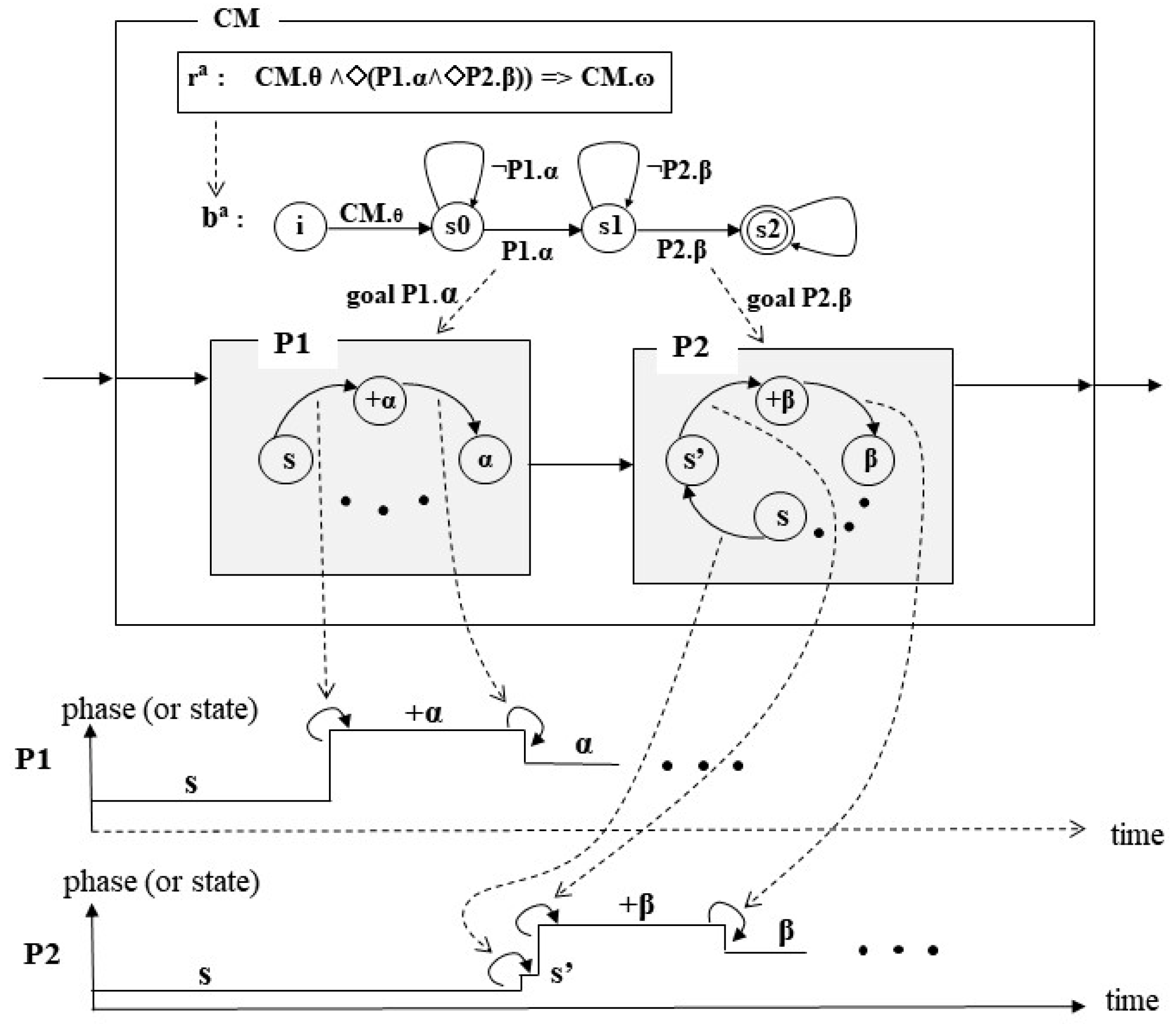
Figure 2 describes how the action rule r^a, after being translated into the Büchi automaton [27,28] b^a, causes the state transitions to reach the subgoals P1.α and P2.β, expressed in the rule condition. State s2, shown in the BA, is the final state, and reaching it indicates the subgoals are completed. Completing the subgoals renders the condition of the rule true and thereafter, the goal of the rule (CM.ω) is reached. Here, P1 and P2 are atomic models.

The BA indicates how and when the component models should have state transitions; that is, it describes that if the current state of the BA is CM.θ, then it transitions to s0, and it transitions to s1 when state α is reached in the P1 model. Likewise, once the BA is at s1, it transitions to s2 when the P2 model reaches state β. Notably, the states in the BA are different from the states of the models. The time taken to reach a subgoal (i.e., how long it takes to transit from one state to the next in the BA) is determined by the corresponding component model appearing in the arc between the two states. The timing diagrams in the lower part of Figure 2 show the instance in which P1 and P2 transition to the next state. There can be more than one subgoal to be achieved by multiple component models associated with the arc. If the component model is an atomic model, the time to reach a subgoal is determined by the model’s selected operation time. Otherwise, if it is a coupled model, the subgoal becomes the goal of an action rule that belongs to the coupled model, which is again recursively regressed to achieve the subgoals of the rule, as explained above. The regression continues until an atomic model, which is located at the bottom level of a hierarchy, is reached.

3.3. Action Execution Algorithm of an Action Rule, TL_ST-DEVS

For each model, a corresponding abstract simulator is created according to the DEVS formalism [1,2]. The abstract simulator is an algorithmic description that indicates how the instructions in a model should be conducted to process the simulation. The ST-DEVS requires a model to be paired with a corresponding abstract simulator because it is extended from DEVS. The action execution algorithm of action rules becomes part of the DEVS abstract simulator, together with the monitoring algorithm of BM-DEVS [6] that is integrated into ST-DEVS.

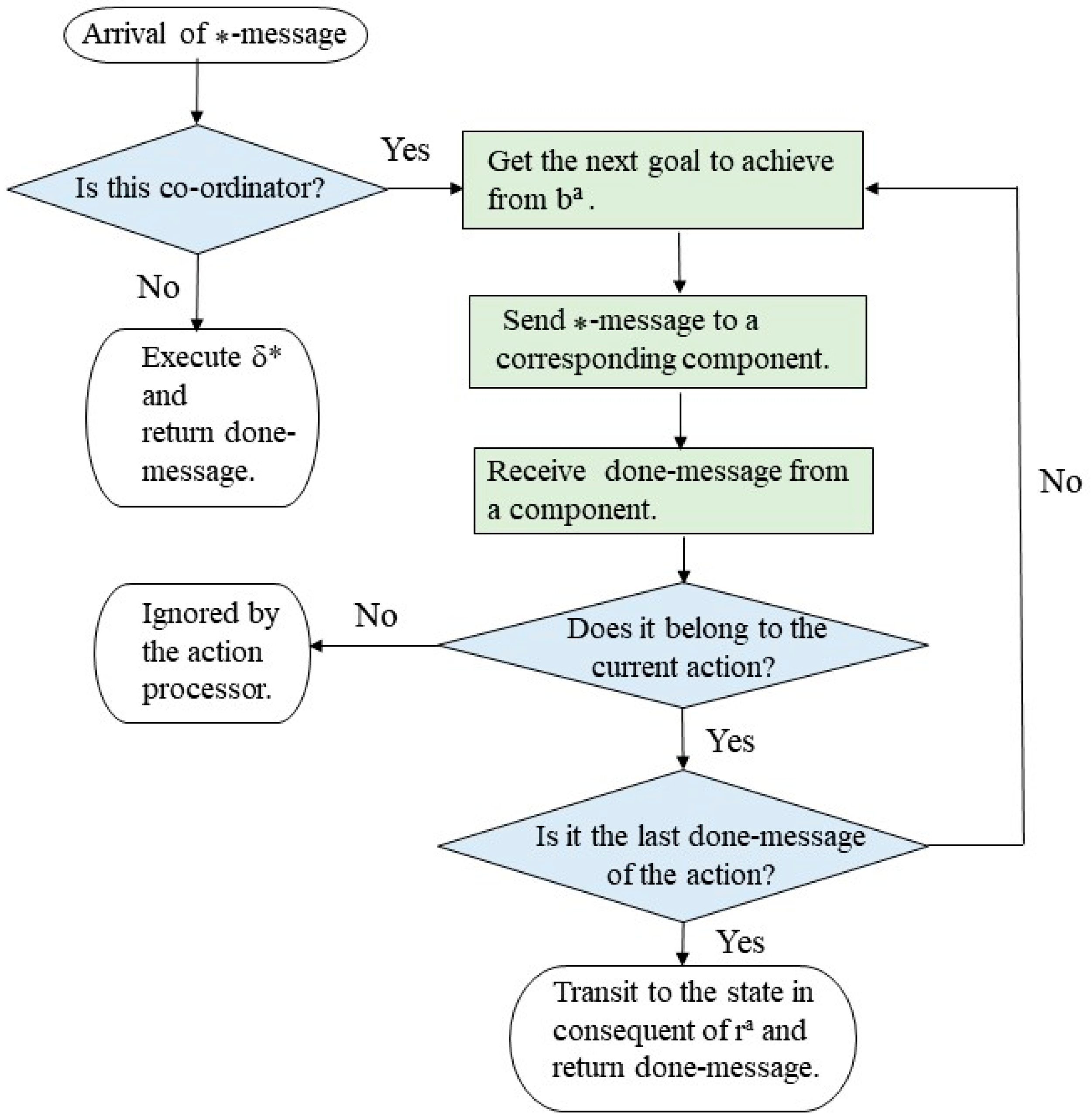
Figure 3 describes how the action execution algorithm operates when executing an action rule through the corresponding automaton b^a, translated from the action rule r^a. The execution algorithm is invoked upon receipt of a ⁎-message [1] from the parent, which delivers a goal in the message to the abstract simulator. If the abstract simulator that receives the message is a coordinator (i.e., an abstract simulator for a coupled model [2]), then the manner in which the goal can be reached is described in b^a. Otherwise, if the abstract simulator is for an atomic model, the goal is achieved by δ* of the model. To trigger the action rule through b^a, the final state of the automaton must be reached. This requires all the preceding states leading to the final state to be reached first, which in turn requires the subgoals associated with the arcs in b^a to be achieved (Figure 2). The subgoals are achieved by issuing ⁎-messages to the corresponding component models. After a ⁎-message is sent to a component, the sender coordinator waits for a done message from the component. The done message [1] is received from a component whenever a ⁎-message is sent to the component. If the received done message is from one of the components that appear in the invoked action rule, namely the rule currently being executed, and it indicates the achievement of the subgoal sent along with the ⁎-message, then the coordinator also checks whether the message is the last done message needed to reach the final state of the automaton b^a. If the final state of b^a is reached, then the corresponding coupled model transitions to the state described in the consequent of action rule r^a. If the done message belongs to the action rule but is not the last done message, then the next ⁎-message is issued to the corresponding component model. If the done message does not belong to the action rule, it is ignored by the action processor or action execution algorithm.

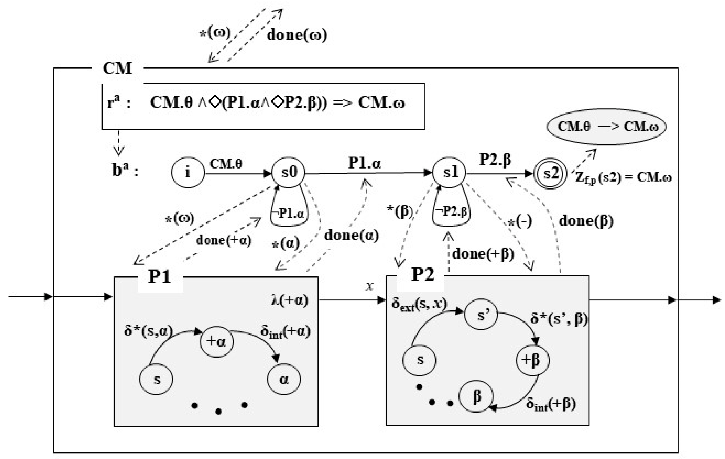
The working of the action execution algorithm is elaborated on by a sequence of procedures that occur during the execution of action rule r^a, CM.θ ˄ ◊ (P1.α ˄ ◊ P2.β) => CM.ω, as shown in Figure 4. The top of the figure shows the arrival of a ⁎-message, ⁎(ω), indicating that the goal of the CM is ω. Because the consequent of the rule is CM.ω, this particular rule is invoked to trigger the antecedent; that is, the goal CM.ω is regressed to cause the antecedent of the rule CM.θ ˄ ◊(P1.α ˄ ◊P2.β) to be true. While triggering the rule, b^a is used until the condition becomes true. If the current state of the CM is θ, then the action execution algorithm sends a ⁎(α) message down to the P1 model, indicating that P1 should achieve the subgoal α. Upon receipt of the message, P1 executes δ* to transition to the +α state; the state name +α describes that it is the state that performs operations necessary to reach the goal state α. Immediately after completing the state transition to +α, done(+α) is returned to the CM from P1 with the current state value of P1, +α. Because P1.+α makes a state transition from s0 to itself, there is no state transition to s1 in b^a. Later, when P1 transits to α, done(α) is sent to the CM, which triggers a state transition from s0 to s1 in b^a. Simultaneously, when P1 transits to α, the output function λ of P1 is executed to deliver its output to the P2 model for subsequent processing. P2 executes its external transition function δ_ext to transition to state s’ after receiving the input sent from P1. Once b^a is in s1, the next message, ⁎ (β), is sent to P2. The rest of the procedure is similar to the case when ⁎(α) was sent. Later, when done(β) arrives at the CM, b^a transitions to its final state s2, which indicates that the condition of the rule r^a is true. Once it becomes true, the CM transitions to the ω state and done(ω) is sent to the parent, indicating that the goal ω is achieved.

The ⁎-message is sent downward from a coupled model and processed at the components recursively until the bottom level is reached, as described previously. The done message is sent upward and processed recursively until the top level is reached within the hierarchy. Notably, because the state transition diagrams of P1 and P2 are not suitable to describe the time-related procedures, the time-valued input of the external-transition function δ_ext and that of the done message are not shown in Figure 4 for the sake of simplicity. The internal transition function δ_int is executed when an atomic model must make a state transition other than those that are due to an input and ⁎-message without a goal, as shown in P1 and P2.

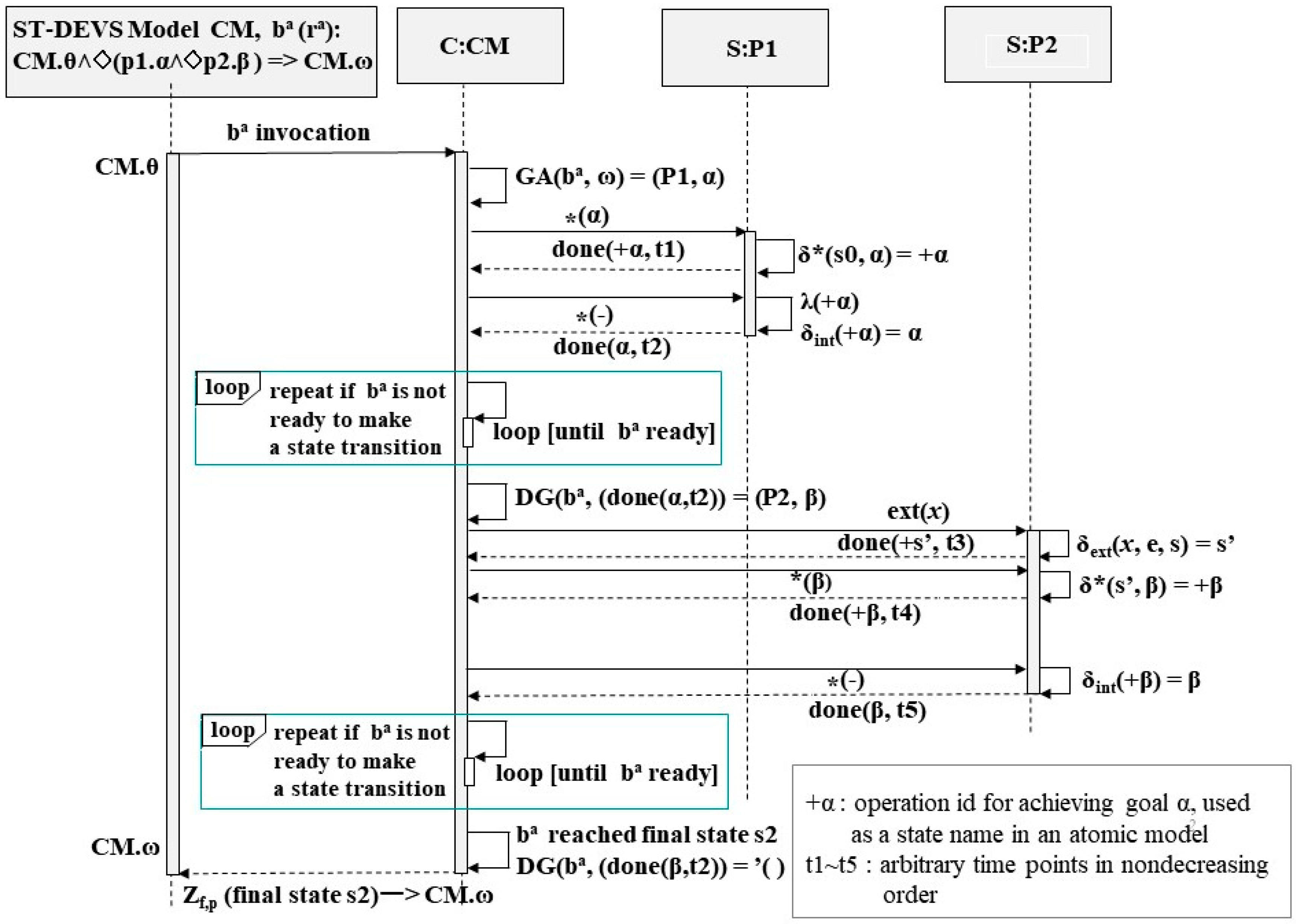
The sequence diagram in Figure 5 describes how action rule r^a is processed over time until the goal of the CM is achieved. The top part of the figure shows four rectangles corresponding to the CM model, C:CM (CM’s abstract simulator), S:P1 (P1’s abstract simulator), and S:P2 (P2’s abstract simulator). The execution of the state transition functions of the models and the necessary processing occurs within the abstract simulator counterparts. The models store state transition functions, state variables, and other information regarding the models. Therefore, when explaining the activities related to a certain model, the abstract simulator and model are not usually distinguished, as shown in the explanation regarding Figure 4. The activities shown in Figure 5 are self-explanatory because the order of the activities is already described in Figure 4. The GA is a goal−to−action rule translation function that determines the action rule to be invoked when a ⁎-message arrives. For example, in Figure 5, the action rule r^a or b^a is invoked when ⁎(ω) arrives. The DG is a done−to−goal translation function that determines the subgoals to be achieved next or where to send the next ⁎-message upon receiving a done message if it is not the last done message. If it is the last message, then DG returns a null value, indicating that the rule is triggered or the final state of b^a is reached. In Figure 5, when done(α, t2) is received from P1, ⁎(β) is sent to P2 as the next message in response to done(α, t2).

4. Example Application of an Action Rule

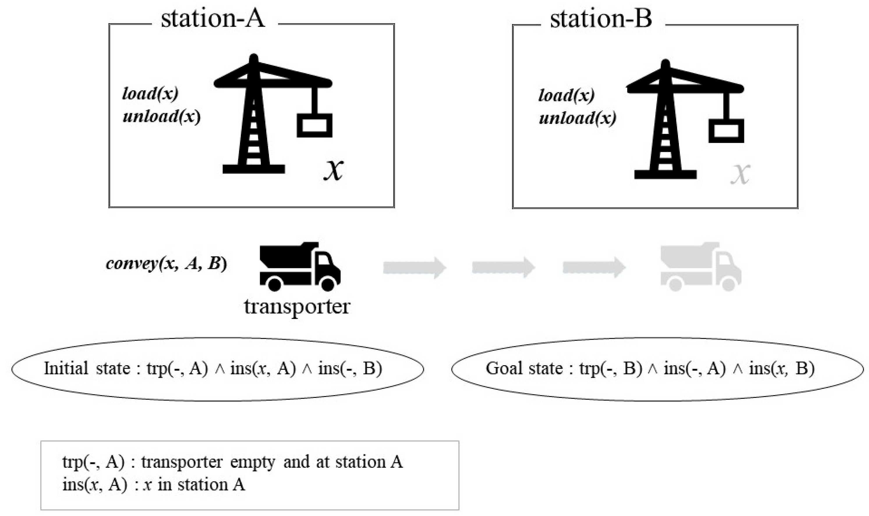
This section describes a simple transportation system with two stations (A and B) and a single transporter (trp), as shown in Figure 6. Each station has a crane that can load and unload an item. The transporter carries an item between the two stations. Initially, both item x and the transporter are in station A. This initial state is expressed by the expression trp(-, A) ∧ ins(x, A) ∧ ins(-, B), where trp(-, A) indicates that the transporter is at A with no item. The ins(x, A) and ins(-, B) predicates indicate that item x is in A and no item is in B, respectively. The goal state to reach is expressed by the expression trp(-, B) ∧ ins(-, A) ∧ ins(x, B), indicating that item x is in B and the transporter is at B with no item. The transitions from ins(x, A) to ins(-, A) and from ins(-, B) to ins(x, B) are performed by the load(x) and unload(x) operations of the crane, respectively. The transition from trp(x, A) to trp(x, B) occurs by the convey(x, A, B) operation of the transporter. The initial state and the goal state are illustrated in black and gray, respectively.

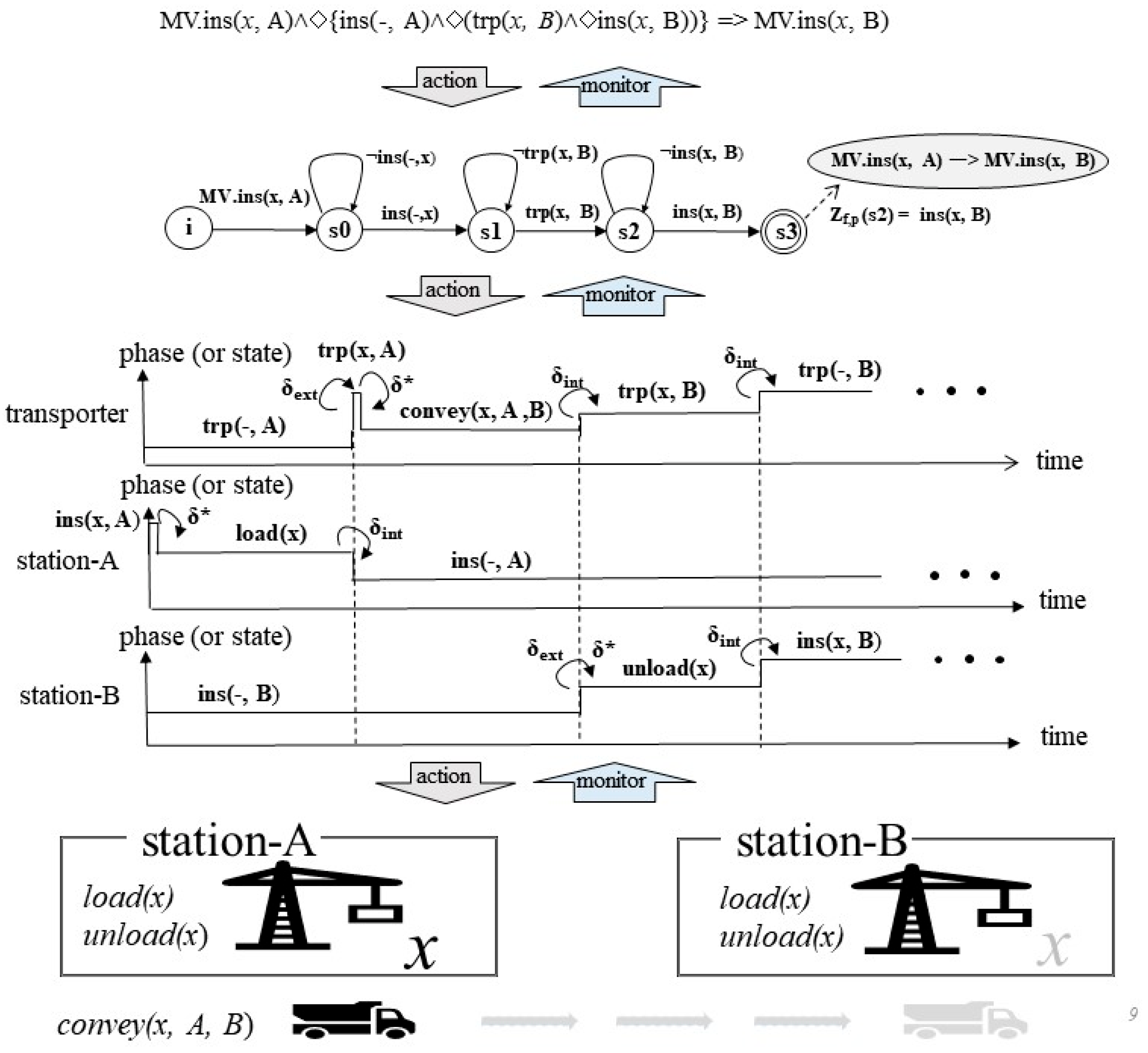
The action rule to be executed for the transportation system is MV.ins(x, A) ˄ ◊{ins(-, A) ˄ ◊(trp(x, B) ˄ ◊ins(x, B))} => MV.ins(x, B). The rule is defined in the MV or mover model so that the model can execute the action rule to reach the goal state described in Figure 6. The MV, not explicitly shown in the figure, is a coupled model whose component models are the transporter, station-A, and station-B. During the action rule execution, the control regarding when and how operations, namely load, unload, and convey, should be performed are determined and applied to the corresponding physical transporter system, as shown in Figure 6. The action rule states that if MV.ins(x, A) is true and the rest of the antecedent of the rule becomes true, then MV.ins(x, B) becomes true, indicating that the goal of the action rule is achieved. As a result of achieving the goal MV.ins(x, B) of the rule, the transportation system goal state trp(-, B) ∧ ins(-, A) ∧ ins(x, B) is reached, as shown in Figure 6.

For the antecedent to become true, MV.ins(x, A) should be true at the current time-instant, and the subgoal ins(-, A) should be achieved in some future; afterward, the subgoal trp(x, B) should be achieved in some future, after which the subgoal ins(x, B) should be achieved in some future. To achieve the subgoal ins(-, A), item x in station-A is removed by the load(x) operation of the crane in station-A after a certain loading time. Consequently, the transporter at A holds item x, which is expressed by trp(x, A). Likewise, the transporter moves to station-B to achieve the subgoal trp(x, B) via the convey(x, A, B) operation after a certain moving time. Finally, the last subgoal ins(x, B) is achieved by the unload(x) operation of the crane in station-B after a certain unloading time. Figure 7 shows the action rule, corresponding BA, sequence of subgoals, and timing diagrams for the three component models of the MV model. Everything down to the timing diagrams belongs to ST-DEVS models, and the corresponding real transportation system that physically performs the load, unload, and convey operations according to the action rule is shown at the bottom. The timing diagrams indicate when and what operations and state transitions are performed in the component models of the MV. The action rule can also be used for monitoring to ensure that the sequence of operations to achieve the subgoals is performed correctly in the physical system. The information flow regarding the action execution is depicted as downward arrows, whereas that of monitoring [6] is depicted as upward arrows.

5. Discussions

Considering that all behaviors in real systems occur in space−time, the behavior-related computation should adopt both time and space as essential elements to ensure a valid representation of the real systems and perform subsequent computations effectively. Therefore, applying a spatiotemporal computation consisting of time-dependent variables and temporal statements that use such variables is a natural approach to solving problems encountered in the target real systems. Because the primary purpose of simulation models is to replicate the dynamics of real systems considering two elements (i.e., time and space), the models are exploited as computation variables in this research. These model-based variables are treated as time-dependent variables because their values are determined according to the passage of time.

5.1. Time-Dependent Variable

When problems are solved using software programs, the most basic and essential activity involves defining data structures or compound variable types to declare variables to represent and solve the problems. If the target problems are related to real systems, then the variables should be able to represent the behavior as well as the structure of these real systems. Thus, the variables should be time-dependent because the behavior occurs within space−time. This study illustrates how ST-DEVS models are exploited in the definition of the TDVs to be used as arguments of the action rules (TL_ST-DEVS) and an action execution algorithm that executes the rules.

The proposed time-dependent variable is a function, such as a fuzzy variable [32] or a random variable [33]. A membership function defined for a fuzzy variable determines the return value to be stored in the fuzzy variable, which is necessary for a fuzzy computation. A density function defined for a random variable determines the return value to be stored in the random variable, which is necessary for a random process. Likewise, an action rule TL_ST-DEVS defined for a time-dependent variable of ST-DEVS determines the return value to be stored in the time-dependent variable, which is necessary for an action execution. If it is a monitoring rule, then the return value necessary for monitoring is stored. Action and monitoring rules express the state trajectories of models, where the trajectories are time−to−state mapping functions. Therefore, the time-dependent variables of ST-DEVS are general-purpose variables that can be used depending on the type of rule in which the time-dependent variable is an argument.

The ST-DEVS defines the time-dependent variables to be used by the TL_ST-DEVS rules. Note that the rules are stored within the variable, variables are used as arguments of the rules, rules are stored within the variables, and so on, which continues until the bottom level variable is reached. That is, the structure of the variable or model is recursively defined to construct a hierarchical modular model or a compound temporal data structure, which is necessary to represent and store the behaviors of complex and large real systems. The hierarchical modular model construction is possible because the proposed formalism is extended from the DEVS [1,2] formalism.

5.2. Important Considerations of ST-DEVS Implementation

ST-DEVS models can also monitor component models to detect important behaviors occurring in the corresponding real system, such as in BM-DEVS [6], which is integrated into ST-DEVS. The integration is performed by embedding the monitoring and action execution algorithms into the abstract simulator [1] and making them cooperate so that identical TL_ST-DEVS rules can be used for both monitoring and action execution. Otherwise, the rules can be separately defined, and monitoring results can be used for initiation of the action execution, or vice versa.

In the BA diagram (Figure 7) of the action rule, there is only one subgoal attached to each arc; however, there can be multiple subgoals attached to an arc to express that the operations for achieving subgoals should be performed in parallel until all the subgoals are met. This scheme is a convenient way of expressing how and when components should act to collaborate in the accomplishment of a complex task or goal. In addition, multiple action rules can be invoked at any moment if conflicts occurring during the execution of rules can be resolved with appropriate strategies. The conflict resolution strategy is straightforward because a model needs to consider its own context only, irrespective of the time constraint being imposed, without considering how other models are performing. At the end of the operation, whether the goal is achieved is only reported as the result to the parent model. It is at the parent model’s discretion to determine how to utilize the result report obtained from the component regarding the action execution that only considers its own context.

In M_ST-DEVS (5) and N_ST-DEVS (6), G, which is a set of goals, is one of the constituent elements of the formalism. G is included in the formalism, even if a model knows what its available goals are, because G is needed for a parent model to define action rules whose arguments are formed by component models and their goals, such as P1.α or P2.β, where α and β are the goals of the P1 and P2 models, respectively. When the goal itself can clearly indicate what the model is, then the argument can be defined by the goal alone (e.g., trp(x, B)), meaning the transporter should be at station-B with item x in it.

The moment ○ is incremented when a done message is received from the component model if the model appears in the invoked action rules or monitoring rules; multiple rules of different types can be invoked at any instant. Both types of rules attempt to achieve their own goals through action execution and monitoring algorithms. The receipt of a done message [1] indicates that a state (or phase) change has occurred, which means that a subgoal has been achieved. If the state change at the component does not achieve one of the subgoals of the rules, incrementing the moment value is unnecessary because the moment value only marks the time-instant related to achieving goals in ST-DEVS, namely the occurrence of important events defined by the modeler. The principle is identical to the definition of important events in an atomic model. The difference is that as we go up along the hierarchy of the model structure, both time and space are abstracted in defining important events.

To achieve a goal (e.g., MV.ins(x. B)) for a coupled model, the subgoals (e.g., ins(-, A), trp(x, B), and ins(x, B)) described in an action rule should be achieved first, as shown in Figure 7. If a component model of the coupled model is an atomic model type, then the subgoal, which is the goal in view of the component, is achieved by performing one of the operations (load(x), convey(x, A, B), or unload(x)) defined in the corresponding component. Otherwise, if a component is a coupled model type, then the subgoal becomes the goal, and a similar process is repeated as in the one described above. If multiple goals are available for an atomic model, then multiple operations are usually required. However, the number of goals does not need to match the number of operations because different goals can be achieved by different combinations of operations.

5.3. Added Functionalities to Classic DEVS

The purpose of the proposed ST-DEVS is to extend the classic DEVS to provide new functionalities that are difficult to obtain by applying DEVS alone. ST-DEVS is not intended to replace any existing functionality of DEVS. As an example, an action rule CM.θ ˄ ◊(P1.α ˄ ◊P2.β) => CM.ω written in a coupled model achieves the goal state (CM.ω) by executing the sequence of sub-actions described in the antecedent of the rule, as shown in Figure 4. The sequence of the sub-actions is carried out by the component models (children models) of the coupled model in which the action rule is written. Therefore, the execution of the action rule involves the coupled model and component models, just as a port coupling information of the coupled model involves these models. Neither the coupling information nor the action rule can be written in an atomic model to effectively achieve the purpose for which they were written. Unlike an atomic model, in which various activities can be written as a transition function and an output function, there is no room to provide activities in a coupled model. This clearly shows the need to extend classic DEVS in order to accommodate the functionality of action executions that this article is proposing. In the action rule, the component models are used as arguments that change their values over time, which makes the argument become a time-dependent variable (TDV). The formal definition of a TDV is described in Section 3 and the necessity and properties of TDVs are elaborated on in Section 5.1

This article shows how an action rule and its execution module are designed to achieve a goal of the rule. The rule and execution module are designed in such a way that when an action rule is executed, it should be able to coordinate with the monitoring rule, defined according to the BM-DEVS [6], so that the proper execution of the action can be monitored. During the monitoring activity, if a certain malfunction or desired behavior is detected, an appropriate action rule should be applied to control the target system. This explains the necessity to include BM-DEVS in ST-DEVS. The former provides the monitoring functionality, and the latter provides the action functionality and coordinates these two types of functionalities.

6. Conclusions and Future Research

The ST in ST-DEVS is an acronym for “spatiotemporal computation,” suggesting that it is a formalism proposed to show how a spatiotemporal computation can be accomplished by an approach in which TDVs are defined, and action rules composed of TDVs are executed. Under this formalism, the statements for monitoring can also be inserted and used to detect occurrences of certain behaviors, as shown in a previous article [6]. Together with the two types of rules, they constitute most of the functions required to operate the software system, such as the digital twin, for online control of the corresponding physical system. In addition to controlling tasks, simulations can be performed using the model to evaluate the performance of the corresponding real system as it is or after applying various new strategies or structural modifications. The proposed approach to solve these problems is designed while considering the symmetry between the real world and the cyberworld, in that both worlds are influenced by time and space.

The main contribution of the proposed methodology is, first, to define ST-DEVS models as TDVs in the representation and storage of temporal as well as spatial data, which is necessary to correctly express problems related to large and complex physical systems that operate in space−time. Second, the composition of an action execution algorithm that illustrates how an action rule (TL_ST-DEVS) can be executed to achieve a goal in the consequent of the rule. The action rule uses the time-dependent variables of the ST-DEVS models as arguments. The action execution algorithm invokes the necessary process to achieve subgoals through a goal regression on the rule, as described in Figure 3, Figure 4, and Figure 5. Notably, the necessary process to achieve the subgoals is given within the arguments, namely the time-dependent variables defined by the ST-DEVS models. This property enables the construction of hierarchical models or compound data structures to store behavioral and structural data required for the monitoring and action-executing. The process of achieving the subgoals is expressed by operations in the component atomic models or action rules in the component coupled models. The spatiotemporal computation proposed is accomplished by time-dependent variables and an execution algorithm that executes action rules (TL_ST-DEVS).

The contributions can be restated in view of DEVS formalism. The direct contribution of the proposed study is to provide the action execution capability to DEVS. In this case, DEVS needs to be extended because it is difficult to achieve such capability with DEVS alone, as explained in Section 5.3. Another contribution is how the extension is done (i.e., on what principle). It is done by defining TDVs, the action rule that uses TDVs as arguments, and the execution module (Section 3). The principle that explains why time-dependent variables should be defined is based on the observation that since all behaviors in real systems occur in space−time, the behavior-related computation should adopt time-dependent variables. These variables store both time and space values as essential elements to ensure a valid representation of the real system and to perform subsequent computations effectively.

In summary, because the purpose of this paper involves solving real world problems through software systems, such as digital twins, more accurate representation of real world problems in these software systems will improve their problem solving capabilities. In other words, since problems in the real world are expressed as values of time and space, it is a very logical result that if variables can express values of time and space as essential properties, the possibility of solving more complex and difficult problems increases. Therefore, the contribution of this study depends on how TDVs are defined and whether it is possible to make use of the TDV in solving useful problems. This article shows problem solving with action executions on simulation models (or digital twins) in such a way that the action can be readily monitored by the previously proposed method shown in BM-DEVS [6]. The definition of TDVs, action instructions using TDVs as input arguments, and a detailed design of the action execution module are described in Section 3. An application example and the problem solving process are described in Section 4.

Future research will include generalizing the application of spatiotemporal computation beyond monitoring and action execution to utilize simulation model-based time-dependent variables in a broader context. Currently, it is not specified how the action rules are initially composed. We assume that the action rules are generated via intelligent planning. By applying the approach suggested in this study, a groundwork for solving intelligent planning problems with time constraints and various conflicts can be formed. Based on this groundwork, future work will involve implementing an intelligent planning agent to compose action rules. In addition, applying the proposed methodology to complex practical applications will be a focus of future research.

References

- Zeigler, B.P. Object-Oriented Simulation with Hierarchical, Modular Models: Intelligent Agents and Endomorphic Systems; Academic Press: San Diego, CA, USA, 1990; pp. 41–143. [Google Scholar]
- Zeigler, B.P.; Muzy, A.; Kofman, E. Theory of Modeling and Simulation: Discrete Event & Iterative System Computational Foundations; Academic Press: San Diego, CA, USA, 2018. [Google Scholar]
- Nance, R.E.; Overstreet, C.M. History of Computer Simulation Software: An Initial Perspective. In Proceedings of the 2017 Winter Simulation Conference, Las Vegas, NV, USA, 3–6 December 2017; pp. 243–261. [Google Scholar]
- Minerva, R.; Lee, G.M.; Crespi, N. Digital Twin in the IoT Context: A Survey on Technical Features, Scenarios, and Architectural Models. Proc. IEEE 2020, 108, 1785–1824. [Google Scholar] [CrossRef]
- Barricelli, B.R.; Casiraghi, E.; Fogli, D. A Survey on Digital Twin: Definitions, Characteristics, Applications, and Design Implications. IEEE Access 2019, 7, 167653–167671. [Google Scholar] [CrossRef]
- Cho, T.H. Simulation Methodology-Based Context-Aware Architecture Design for Behavior Monitoring of Systems. Symmetry 2020, 12, 1568. [Google Scholar] [CrossRef]
- Metz, S. Practical Object-Oriented Design, 2nd ed.; Addison-Wesley: Boston, MA, USA, 2018. [Google Scholar]
- Forouzan, B.A.; Gilberg, R.F. C++ Programming: An Object-Oriented Approach; McGraw-Hill: New York, NY, USA, 2019. [Google Scholar]
- Heagerty, P.J.; Lumley, T.; Pepe, M.S. Time-Dependent ROC Curves for Censored Survival Data and a Diagnostic Marker. Biometrics 2000, 56, 337–344. [Google Scholar] [CrossRef] [PubMed]
- Hoering, A.; Crowley, J.; Shaughnessy, J.D., Jr.; Hollmig, K.; Alsayed, Y.; Szymonifka, J.; Waheed, S.; Nair, B.; Rhee, F.V.; Anaissie, E.; et al. Complete remission in multiple myeloma examined as time-dependent variable in terms of both onset and duration in Total Therapy protocols. Clin. Trials Obs. 2009, 114, 1299–1305. [Google Scholar] [CrossRef] [PubMed]
- Adhikari, S.; Billing, G.D. A time-dependent discrete variable representation method. J. Chem. Phys. 2000, 113, 1409–1414. [Google Scholar] [CrossRef]
- Cheskes, S.; Schmicker, R.H.; Rea, T.; Powell, J.; Drennana, I.R.; Kudenchuk, P.; Vaillancourt, C.; Conwaye, W.; Stiell, I.; Stubg, D.; et al. Chest compression fraction: A time dependent variable of survival in shockable out-of-hospital cardiac arrest. Resuscitation 2015, 97, 129–135. [Google Scholar] [CrossRef] [PubMed]
- Jung, S.Y.; Jo, H.; Son, H.; Hwang, H.J. Real-World Implications of a Rapidly Responsive COVID-19 Spread Model with Time-Dependent Parameters via Deep Learning: Model Development and Validation. J. Med. Internet Res. 2020, 22, e19907. [Google Scholar] [CrossRef] [PubMed]
- Jitkajornwanich, K.; Pant, N.; Fouladgar, M.; Elmasri, R. A survey on spatial, temporal, and spatio-temporal database research and an original example of relevant applications using SQL ecosystem and deep learning. J. Inf. Telecommun. 2020, 4, 524–559. [Google Scholar] [CrossRef]
- Bakli, M.; Sakr, M.; Soliman, T.H.A. HadoopTrajectory: A Hadoop spatiotemporal data processing extension. J. Geogr. Syst. 2019, 21, 211–235. [Google Scholar] [CrossRef]
- Wen, Y.H.; Gao, L.; Fu, H.; Zhang, F.L.; Xia, S. Graph CNNs with Motif and Variable Temporal Block for Skeleton-Based Action Recognition. In Proceedings of the Thirty-Third AAAI Conference on Artificial Intelligence, Honolulu, HI, USA, 27 January–1 February 2019. [Google Scholar]
- Shi, Z.; Pun-Cheng, L.S.C. Spatiotemporal Data Clustering: A Survey of Methods. ISPRS Int. J. Geo-Inf. 2019, 8, 112. [Google Scholar] [CrossRef] [Green Version]
- Largouët, C.; Krichen, O.; Zhao, Y. Temporal Planning with extended Timed Automata. In Proceedings of the 2016 IEEE 28th International Conference on Tools with Artificial Intelligence, San Jose, CA, USA, 6–8 November 2016. [Google Scholar]
- Bernardini, S.; Fox, M.; Long, D. Combining temporal planning with probabilistic reasoning for autonomous surveillance missions. Auton Robot. 2017, 41, 181–203. [Google Scholar] [CrossRef] [PubMed] [Green Version]
- Moon, S.I.; Lee, K.H.; Lee, D. Fuzzy Branching Temporal Logic. IEEE Trans. Syst. Man Cybern. Part B Cybern. 2004, 34, 1045–1055. [Google Scholar] [CrossRef] [PubMed]
- Lamine, K.B.; Kabanza, F. History checking of temporal fuzzy logic formulas for monitoring behavior-based mobile robots. In Proceedings of the International Conference on Tools with Artificial Intelligence, Baltimore, MD, USA, 9–11 November 2000. [Google Scholar]
- Ko, H.; Lee, J.; Pack, S. Spatial and Temporal Computation Offloading Decision Algorithm in Edge Cloud-Enabled Heterogeneous Networks. IEEE Access 2018, 6, 18920–18932. [Google Scholar] [CrossRef]
- Pnueli, A. The Temporal Logic Of Program. In Proceedings of the 18th Annual Symposium on Foundations of Computer Science, Providence, RI, USA, 31 October–2 November 1977. [Google Scholar]
- Cristiá, M.; Zeigler, B.P. Formalizing the semantics of modular DEVS models with temporal logic. In Proceedings of the 7e Conférence Francophone de MOdlisation et SIMulation-MOSIM, Paris, France, 31 March–2 April 2008; Volume 8. [Google Scholar]
- Mordechai, B.A.; Pnueli, A.; Manna, Z. The temporal logic of branching time. Acta Inform. 1983, 20, 207–226. [Google Scholar]
- Fisher, M. An Introduction to Practical Formal Methods Using Temporal Logic; John Wiley & Sons: Hoboken, NJ, USA, 2011; pp. 12–48. [Google Scholar]
- Büchi, J.R. The Collected Works of J. Richard Büchi; Springer Science & Business Media: Berlin, Germany, 2012. [Google Scholar]
- Büchi, J.R. On a decision method in restricted second order arithmetic. In The Collected Works of J. Richard Büchi; Mac Lane, S., Siefkes, D., Eds.; Springer: New York, NY, USA. [CrossRef]
- Sipser, M. Introduction to the Theory of Computation, 3rd ed.; Cengage Learning: Boston, MA, USA, 2012. [Google Scholar]
- Hopcroft, J.E.; Motwani, R.; Ullman, J.D. Introduction to Automata Theory, Languages, and Computation, 3rd ed.; Pearson: Chennai, India, 2008. [Google Scholar]
- Kolman, B.; Busby, R.; Ross, S. Discrete Mathematical Structures, 6th ed; Pearson: London, UK, 2017. [Google Scholar]
- Zadeh, L.A. Information and Control. Fuzzy Sets 1965, 8, 338–353. [Google Scholar]
- DeGroot, M.H.; Schervish, M.J. Probability and Statistics, 4th ed.; Pearson: London, UK, 2011. [Google Scholar]
Figure 1.
Example of action rule, TLST-DEVS, and corresponding Büchi automaton.
Figure 2.
Execution of action rule, TLST-DEVS.
Figure 3.
Flow chart of the action execution process.
Figure 4.
Action rule, CM.θ ˄ ◊ (P1.α ˄ ◊ P2.β) => CM.ω, execution and abstract simulator messages.
Figure 5.
Sequence diagram of action rule execution, CM.θ ˄ ◊(P1.α ˄ ◊P2.β) => CM.ω.
Figure 6.
Transportation system with two stations and a single transporter.
Figure 7.
Execution of an action rule that conveys an item from station-A to station-B.
Publisher’s Note: MDPI stays neutral with regard to jurisdictional claims in published maps and institutional affiliations. |
© 2022 by the author. Licensee MDPI, Basel, Switzerland. This article is an open access article distributed under the terms and conditions of the Creative Commons Attribution (CC BY) license (https://creativecommons.org/licenses/by/4.0/).
Share and Cite
MDPI and ACS Style
Cho, T. ST-DEVS: A Methodology Using Time-Dependent-Variable-Based Spatiotemporal Computation. Symmetry 2022, 14, 912. https://0-doi-org.brum.beds.ac.uk/10.3390/sym14050912
AMA Style
Cho T. ST-DEVS: A Methodology Using Time-Dependent-Variable-Based Spatiotemporal Computation. Symmetry. 2022; 14(5):912. https://0-doi-org.brum.beds.ac.uk/10.3390/sym14050912
Chicago/Turabian StyleCho, Taeho. 2022. "ST-DEVS: A Methodology Using Time-Dependent-Variable-Based Spatiotemporal Computation" Symmetry 14, no. 5: 912. https://0-doi-org.brum.beds.ac.uk/10.3390/sym14050912
Note that from the first issue of 2016, this journal uses article numbers instead of page numbers. See further details here.