Novel Aczel–Alsina Operators for Pythagorean Fuzzy Sets with Application in Multi-Attribute Decision Making

Abstract

Multi-attribute decision-making (MADM) is usually used to aggregate fuzzy data successfully. Choosing the best option regarding data is not generally symmetric on the grounds that it does not provide complete information. Since Aczel-Alsina aggregation operators (AOs) have great impact due to their parameter variableness, they have been well applied in MADM under fuzzy construction. Recently, the Aczel-Alsina AOs on intuitionistic fuzzy sets (IFSs), interval-valued IFSs and T-spherical fuzzy sets have been proposed in the literature. In this article, we develop new types of Pythagorean fuzzy AOs by using Aczel-Alsina t-norm and Aczel-Alsina t-conorm. Thus, we give these new operations Aczel-Alsina sum and Aczel-Alsina product on Pythagorean fuzzy sets based on Aczel-Alsina t-norm and Aczel-Alsina t-conorm. We also develop new types of Pythagorean fuzzy AOs including Pythagorean fuzzy Aczel-Alsina weighted averaging and Pythagorean fuzzy Aczel-Alsina weighted geometric operators. We elaborate some characteristics of these proposed Aczel-Alsina AOs on Pythagorean fuzzy sets, such as idempotency, monotonicity, and boundedness. By utilizing the proposed works, we solve an example of MADM in the information of the multinational company under the evaluation of impacts in MADM. We also illustrate the comparisons of the proposed works with previously existing AOs in different fuzzy environments. These comparison results demonstrate the effectiveness of the proposed Aczel-Alsina AOs on Pythagorean fuzzy sets.

1. Introduction

Multi-attribute decision making (MADM) is one of most notable parts of decision making (DM). It plans to choose the most reasonable option from a set of alternatives within the sight of different standards that frequently struggle with one another. With the hesitation of DM subjects and the fluffiness of DM conditions, MADM is acknowledged as a significant method due to its simple appropriateness. To solve such issues with vague data, fuzzy sets (FSs) was introduced in [1] where the truth grade (TG) of a component of a set was characterized by a framework on $\left[0, 1\right]$, and the falsity grade (FG) could be obtained by subtracting the TG from $1$. The fuzzy set theory has been widely applied in various areas, such as Yang et al. [2,3]. Atanassov [4] built on Zadeh’s idea of FSs to intuitionistic fuzzy sets (IFSs), where the TG $“\mu ”$ and FG $“\nu ”$ are characterized autonomously, but with the significant requirement that their sum must be in $\left[0, 1\right]$, i.e., $sum \left(\mu ,\nu \right)\in \left[0, 1\right]$. Furthermore, the term $1-sum\left(\mu , \nu \right)$ was referred to as hesitancy grade,$ř (ẇ)$. Due to the limitation of Atanassov’s model of IFS, TG and FG cannot be assigned to their characteristic function, as in some cases the sum $\left(\mu ,\nu \right)$ maximizes on$\left[0, 1\right]$. Hence, Yager [5] proposed the concept of Pythagorean FSs (PyFSs), developing the idea of IFSs as the essential of PyFSs becoming $sum \left({\mu }^2, {\nu }^2\right)\in \left[0,1\right]$. The range for the TG and FG of IFSs and PyFSs is portrayed in Figure 1. For the improvements in this case, we refer readers to [6,7,8,9].

Triangular norms play a significant role and are the reason for many AOs discussed in several fuzzy frameworks. Menger [10] discovered the idea of triangular norms statistical information. Deschrijver et al. [11] discussed the idea of t-norm (TN) and t-conorm (TCN) in the environment of IFSs. Various triangular norms were introduced to aggregate the information in different mathematical frameworks. To solve different MADM problems, aggregation of information plays an important role. There is a variety of TN and TCN that has been used for the aggregation of information at a large scale. These TN and TCN include Lukasiewicz TN and TCN [12], product TN and probabilistic sum TCN [13], Archimedian TN and TCN [14], drastic TN and TCN [15], Einstien TN and TCN [16], and Dombi TN and TCN [17]. These various triangular norms play a significant role in the formation of several AOs. Algebraic TN and TCN lead to the formation of averaging and geometric AOs of IFSs by Xu [18], AOs of PyFSs by Rahman et al. [19], AOs of q-ROF sets by Liu and Wang [20], AOs of interval-valued PyFSs by Garg [21], AOs of T-spherical FSs by Mahmood et al. [22], and AOs of complex T-spherical FSs by Ali et al. [23]. Dombi TN and TCN lead to the development of averaging and geometric AOs of PyFSs by Akram et al. [24] of spherical FSs by Ashraf [25]. Furthermore, some AOs have been developed under Einstine and Frank TN and TCN, such as IFSs by Wang and Liu [26], PyFS by Khan et al. [27], PyFSs by Xing et al. [28], q-ROFSs by Seikh and Mandal [29] and interval-valued picture FSs by Mahmood et al. [30].

In 1982, Aczel and Alsina [31] introduced a new family of TN and TCN called Aczel–Alsina (AA) TN (AA-TN) and TCN (AA-TCN) for a given condition $0\le p\le +\infty$. The AA-TN and AA-TCN are strictly increasing and continuous when the value of $p$ is increases. Many researchers have used the concepts of AA-TN and AA-TCN in different fields to find the superiority of changing active parameters. Babu and Ahmed [32] considered different triangular norms of parametric TN, product TN, Dombi product TN, AA-TN, Frank product TN, and Schweizer and Sklar TN. In Babu and Ahmed [32], they concluded that the AA-TN produces better results. Fahimeh and Mahdi [33] worked on different TN to investigate the effect in the fuzzy rule under the classification environment in which they made experimental comparisons using twelve different data sets and showed that the AA operators have the best performance. Recently, Senapati et al. [34] considered the IF AOs based on the AA-TN and AA-TCN for the selection of human resources by using the MADM problem, and Senapati et al. [35] gave the interval-valued IF AOs based on the AA operations with its selection process of researchers for the renewed university by using the MADM problem. Hussain et al. [36] considered the AA AOs on T-spherical fuzzy sets (TSFSs) with its application to the TSF MADM.

Due to the fact in [33] that AA-TN can produce optimum results in classification and also the behaviors of PyFSs, the goal of this paper is to propose some AA AOs in the frame of PyFSs. We develop a new type of Pythagorean fuzzy (PyF) AOs (PyF-AOs) by using the AA-TN and AA-TCN. Thus, the main purpose of this paper is to develop the notions of PyF AA weighted average (PyF-AA-WA) and PyF AA weighted geometric (PyF-AA-WG) AOs in the environment of PyFSs. We also demonstrate the benefits of the PyF-AA-WA and PyF-AA-WG. Overall, the main contributions of this paper are as follows:

• To study the basic operations of AA-TN and AA-TCN for developing new AOs, such as PyF-AA-WA, PyF-AA-WG, PyF-AA-OWA, PyF-AA-HWA in the framework of PyFSs, and basic operations.
• Some special cases of the proposed AOs are also explored, such as the properties of Idempotency, Monotonicity, and boundedness.
• A MADM technique is used to solve a problem in the selection of applicants for some vacant posts in a multinational company.
• To find the reliability and feasibility of the proposed work, we discuss some numerical examples based on the PyF information.
• In a comparative study, we compare previously existing AOs with our proposed AOs. We comprehensively summarize these comparison results that demonstrate the effectiveness of these proposed AOs.

The remainder of this paper is organized as follows. In Section 2, we review the notion of triangular TN, AA-TN and AA-TCN, PyFSs, and PyF-WA AOs. In Section 3, we discuss the AA operations under PyFSs with their fundamental operations. In Section 4, we propose the PyF-AA-WA OAs in the environment of PyFSs and give their basic properties. In Section 5, we explore the notion of the PyF-AA-WG OAs according to the AA operations on PyFSs. In Section 6, the MADM technique is presented under the proposed work based on the PyFS environment. To find the reliability and feasibility of the proposed AOs, we discuss a numerical example of the selection of employees for a multinational company. In Section 7, a comparative study of the proposed works with previous existing AOs is made. In Section 8, we make our conclusions.

2. Preliminaries

In this section, we elaborate on some basic definitions of TN and TCN for further development of this paper. We also discuss the notion of PyFSs and some basic operations. We recall the definitions of score function and accuracy function.

Definition 1.

A TN is a function$Ŧ:\left[0, 1\right]\times \left[0, 1\right]\to \left[0, 1\right]$that satisfies the property of symmetry, monotonicity, and associativity, and has an identity element, i.e., for all$a, ḅ, c\in \left[0,1\right]$: [10]

(1)

$Ŧ\left(a, ḅ\right)=Ŧ\left(ḅ,a\right);$

(2)

$Ŧ\left(a, ḅ\right)\le Ŧ\left(a, c\right)$ if $ḅ<c;$

(3)

$Ŧ\left(a, Ŧ\left(ḅ, c\right)\right)=Ŧ\left(Ŧ\left(a, ḅ\right), c\right);$

(4)

$Ŧ\left(a, 1\right)=a.$

Example 1.

Some well-known TNs are listed below.

(1)

MinimumTN ${Ŧ}_{min}\left(a, ḅ\right)=min\left(a, ḅ\right);$

(2)

ProductTN ${Ŧ}_{pro}\left(a, ḅ\right)=a ḅ$;

(3)

LukasiewiczTN ${Ŧ}_{Luk}\left(a, ḅ\right)=max\left(a+ḅ-1, 0\right);$

(4)

DrasticTN ${Ŧ}_D\left(a, ḅ\right)=\left(\begin{array}{c}a, if a=1\\ ḅ, if ḅ=1\\ 0, otherwise\end{array}\right) ;$

(5)

Nilpotent minimum${Ŧ}_{nM}\left(a, ḅ\right)=\left(\begin{array}{c}\left(a,ḅ\right) if a+ḅ>1\\ 0, otherwise\end{array}\right).$

Definition 2.

Ref. [37] A TCN is a function $Ṥ:\left[0, 1\right]\times \left[0, 1\right]\to \left[0, 1\right]$ that satisfies the property of symmetry, monotonicity and associativity, and has an identity element, i.e., for all $a, ḅ, c\in \left[0,1\right]$:

(1)

$Ṥ\left(a, ḅ\right)=Ṥ\left(ḅ,a,\right);$

(2)

$Ṥ\left(a, ḅ\right)\le Ṥ\left(a, c\right)$if$ḅ<c;$

(3)

$Ṥ\left(a, Ṥ\left(ḅ, c\right)\right)=Ṥ\left(Ṥ\left(a, ḅ\right), c\right);$

(4)

$Ṥ\left(a, 0\right)=a$.

Example 2.

Some well-known TCNs are listed below.

(1)

MaximumTCN ${Ṥ}_{max}\left(a, ḅ\right)=max\left(a, ḅ\right);$

(2)

Probabilistic sum${Ṥ}_{sum}\left(a, ḅ\right)=a+ḅ-a ḅ$;

(3)

Bounded sum${Ṥ}_{Luk}\left(a, ḅ\right)=\mathit{min}\left\{a+ḅ, 1\right\}$;

(4)

DrasticTCN ${Ṥ}_D\left(a, ḅ\right)=\left(\begin{array}{c}ḅ if a=0\\ a if ḅ=0\\ 1 otherwise\end{array}\right);$

(5)

Nilpotent maximum${Ṥ}_{nM}\left(a, ḅ\right)=\left(\begin{array}{c}max\left(a,ḅ\right) if a+ḅ<1\\ 1, otherwise\end{array}\right)$.

Now, we give the notion of the A-A TN and TCNs defined by Aczél and Alsina [31] in 1982.

Definition 3.

Ref. [31] The AA TN and TCN are defined as follows: $\forall , 0\le ῳ\le +\infty$:

• ${Ŧ}_{Ấ}^{ῳ}\left(a, ḅ\right)=\left\{\begin{array}{c}{Ŧ}_D\left(a, ḅ\right) if ῳ=0\\ min\left(a, ḅ\right) if ῳ=\infty \\ e^{-{({\left(-loga\right)}^{ῳ}+{\left(-logḅ\right)}^{ῳ})}^{\frac{1}{ῳ}}} otherwise\end{array}\right\}$and
• ${Ṥ}_{Ấ}^{ῳ}\left(a, ḅ\right)=\left\{\begin{array}{c}{Ṥ}_D\left(a, ḅ\right) if ῳ=0\\ max\left(a, ḅ\right) if ῳ=\infty \\ 1-e^{-{({\left(-loga\right)}^{ῳ}+{\left(-logḅ\right)}^{ῳ})}^{\frac{1}{ῳ}}} otherwise\end{array}\right\}$, respectively.

Remark 1.

The AA TNs and TCNs can reduce to:

(a)

DrasticTNandTCN: If$ῳ=0$, then${Ŧ}_{Ấ}^0={Ŧ}_D$and${Ṥ}_{Ấ}^0={Ṥ}_{D,}.$

(b)

ProductTNandTCN: If$ῳ=1$then${Ŧ}_{Ấ}^1={Ŧ}_{pro}$and${Ṥ}_{Ấ}^1={Ṥ}_{pro}$.

(c)

MinTNand maxTCN: if$ῳ\to 0$then${Ŧ}_{Ấ}^{\infty }=min$and${Ṥ}_{Ấ}^{\infty }=max$.

Note: The AA TNs and TCNs are two strictly increasing and decreasing functions, respectively.

We next discuss the idea of PyFSs in which the sum of squares of TG and FG is in$\left[0,1\right]$. Moreover, we elaborate on some fundamental operations as given below. The concept of PyFSs was introduced by Yager [5].

Definition 4.

Ref. [5] Consider a non-empty set $Ẁ$. Then, a PyFS $a$ is in the form:

$$a=\left\{\left({\mu }_a(ẇ),{\nu }_a(ẇ)\right)|ẇ\in Ẁ\right\}$$

where ${\mu }_a(ẇ): Ẁ\to \left[0,1\right]$ and ${\nu }_a(ẇ): Ẁ\to \left[0,1\right]$ denote the TG and FG of $ẇ\in Ẁ,$ respectively, provided that $0\le {\mu }_a^2(ẇ)+{\nu }_a^2(ẇ)\le 1$ and hesitancy degree denoted by ${ř}_a(ẇ)=1-\left(\sqrt{{\mu }_a^2(ẇ)+{\nu }_a^2(ẇ)}\right),$ ${ř}_a(ẇ)\in \left[0,1\right], \forall ẇ\in Ẁ$.

Now, we present some basic operations on PyFSs as follows.

Definition 5.

Ref. [38] Consider two PyFSs $Ẋ=\left({\mu }_{Ẋ}(ẇ),{\nu }_{Ẋ}(ẇ)\right)$ and$Ẏ=\left({\mu }_{Ẏ}(ẇ),{\nu }_{Ẏ}(ẇ)\right)$on the universal set$Ẁ$. Then:

(1)

$Ẋ\subseteq Ẏ$, if${\mu }_{Ẋ}(ẇ)\le {\mu }_{Ẏ}(ẇ),{\nu }_{Ẋ}(ẇ)\ge {\nu }_{Ẏ}(ẇ),\forall ẇ\in Ẁ$.

(2)

$Ẋ=Ẏ$, if$Ẋ\subseteq Ẏ$and$Ẋ\supseteq Ẏ$.

(3)

$Ẋ\cup Ẏ=\left\{\max \left({\mu }_{Ẋ}(ẇ),{\mu }_{Ẏ}(ẇ)\right), \min \left({\nu }_{Ẋ}(ẇ),{\nu }_{Ẏ}(ẇ)\right) |ẇ\in Ẁ\right\}$

(4)

$Ẋ\cap Ẏ=\left\{\min \left({\mu }_{Ẋ}(ẇ),{\mu }_{Ẏ}(ẇ)\right), \max \left({\nu }_{Ẋ}(ẇ),{\nu }_{Ẏ}(ẇ)\right) |ẇ\in Ẁ\right\}$

(5)

${Ẋ}^c=\left({\nu }_{Ẋ}(ẇ), {\mu }_{Ẋ}(ẇ)\right), \forall ẇ\in Ẁ$.

Definition 6.

Ref. [38] Let $Ẋ=\left({\mu }_{Ẋ}(ẇ),{\nu }_{Ẋ}(ẇ)\right)$ and $Ẏ=\left({\mu }_{Ẏ}(ẇ),{\nu }_{Ẏ}(ẇ)\right)$ be two PyFSs and $\alpha >0$. Then, some fundamental operational laws are defined as:

(1)

$Ẋ\oplus Ẏ=\left(\sqrt{{\mu }_{Ẋ}^2(ẇ)+{\mu }_{Ẏ}^2(ẇ)-{\mu }_{Ẋ}^2(ẇ).{\mu }_{Ẏ}^2(ẇ)}, {\nu }_{Ẋ}(ẇ).{\nu }_{Ẏ}(ẇ)\right)$

(2)

$Ẋ⨂Ẏ=\left({\mu }_{Ẋ}(ẇ).{\mu }_{Ẏ}(ẇ)\sqrt{{\nu }_{Ẋ}^2(ẇ)+{\nu }_{Ẏ}^2(ẇ)-{\nu }_{Ẋ}^2(ẇ).{\nu }_{Ẏ}^2(ẇ)}\right)$

(3)

$\alpha Ẋ=\left(\sqrt{1-{\left(1-{\mu }_{Ẋ}^2(ẇ)\right)}^{\alpha }, }{\nu }_{Ẋ}^{\alpha }(ẇ)\right)$

(4)

${Ẋ}^{\alpha }=\left( {\mu }_{Ẋ}^{\alpha }, \sqrt{1-{\left(1-{\nu }_{Ẋ}^2(ẇ)\right)}^{\alpha } }\right)$

Definition 7.

Let$Ẋ=\left({\mu }_{Ẋ}(ẇ),{\nu }_{Ẋ}(ẇ)\right)$and$Ẏ=\left({\mu }_{Ẏ}(ẇ),{\nu }_{Ẏ}(ẇ)\right)$be two PyFSs. Then, the generalization of intersection and union of two PyFSs are defined as follows:

(1)

$Ẋ{\cup }_{Ŧ, Ṥ}Ẏ=\left\{Ṥ \left({\nu }_{Ẋ}(ẇ),{\nu }_{Ẏ}(ẇ)\right), Ŧ \left({\mu }_{Ẋ}(ẇ),{\mu }_{Ẏ}(ẇ)\right) |ẇ\in Ẁ\right\}$

(2)

$Ẋ{\cap }_{Ŧ, Ṥ}Ẏ=\left\{Ŧ \left({\mu }_{Ẋ}(ẇ),{\mu }_{Ẏ}(ẇ)\right), Ṥ \left({\nu }_{Ẋ}(ẇ),{\nu }_{Ẏ}(ẇ)\right) |ẇ\in Ẁ\right\}$

where$Ŧ$and$Ṥ$represent the TN and TCN, respectively.

Peng and Yang [38] elaborated on the union and intersection of two PyFSs from the maximum TCNs ${Ṥ}_{max}$ and minimum TN ${Ŧ}_{min}$, respectively. Peng and Yang [38] also investigated the algebraic product and algebraic sum from the algebraic product ${Ŧ}_{pro}$ and algebraic sum of ${Ṥ}_{pro}$, respectively. Since$Ẋ=\left({\mu }_{Ẋ}(ẇ),{\nu }_{Ẋ}(ẇ)\right)$ is a PyF number (PyFN) in which the sum of the square of TG and FG lies in the interval $\left[0,1\right],$ provide that$0\le {\mu }_{Ẋ}^2(ẇ)+{\nu }_{Ẋ}^2(ẇ)\le 1$. Let us consider the three PyFSs of$Ẋ=\left({\mu }_{Ẋ}(ẇ),{\nu }_{Ẋ}(ẇ)\right)$, ${Ẋ}_1=\left({\mu }_{{Ẋ}_1}(ẇ),{\nu }_{{Ẋ}_1}(ẇ)\right)$ and ${Ẋ}_2=\left({\mu }_{{Ẋ}_2}(ẇ),{\nu }_{{Ẋ}_2}(ẇ)\right)$. Then, some fundamental basic operations are defined as

(1)

${Ẋ}_1\subseteq {Ẋ}_2$, if${\mu }_{{Ẋ}_1}\le {\mu }_{{Ẋ}_2},{\nu }_{{Ẋ}_1}\ge {\nu }_{{Ẋ}_2}$.

(2)

${Ẋ}_1={Ẋ}_2$, if${Ẋ}_1\subseteq {Ẋ}_2$and${Ẋ}_1\supseteq {Ẋ}_2$.

(3)

${Ẋ}_1\cup {Ẋ}_2=\left\{\mathit{max} \left({\mu }_{{Ẋ}_1}(ẇ),{\mu }_{{Ẋ}_2}(ẇ)\right), min \left({\nu }_{{Ẋ}_1}(ẇ),{\nu }_{{Ẋ}_2}(ẇ)\right)\right\}$.

(4)

${Ẋ}_1\cap {Ẋ}_2=\left\{min \left({\mu }_{{Ẋ}_1}(ẇ),{\mu }_{{Ẋ}_2}(ẇ)\right), \mathit{max} \left({\nu }_{{Ẋ}_1}(ẇ),{\nu }_{{Ẋ}_2}(ẇ)\right)\right\}$.

(5)

${Ẋ}^c=\left\{\left({\nu }_{Ẋ}(ẇ), {\mu }_{Ẋ}(ẇ)\right), \right\}$.

(6)

$\alpha Ẋ=\sqrt{1-{\left(1-{\mu }_{Ẋ}^2(ẇ)\right)}^{\alpha }, }{\left({\nu }_{Ẋ}(ẇ)\right)}^{\alpha }, \alpha >0$.

(7)

${Ẋ}^{\alpha }={\left({\mu }_{Ẋ}(ẇ)\right)}^{\alpha }, \sqrt{1-{\left(1-{\nu }_{Ẋ}^2(ẇ)\right)}^{\alpha } }, \alpha >0.$

Definition 8.

Ref. [38] Let $Ẋ=\left({\mu }_{Ẋ}(ẇ),{\nu }_{Ẋ}(ẇ)\right)$ be any PyFS. Then, the score function is defined as:

$$\mathcal{S}(Ẋ)={\mu }_{Ẋ}^2(ẇ)-{\nu }_{Ẋ}^2(ẇ), \mathcal{S}(Ẋ)\in \left[0,1\right]$$

(1)

Definition 9.

Ref. [38] Let $Ẋ=\left({\mu }_{Ẋ}(ẇ),{\nu }_{Ẋ}(ẇ)\right)$ be any PyFS. Then, the accuracy function is defined as:

$$\mathcal{A}(Ẋ)={\mu }_{Ẋ}^2(ẇ)+{\nu }_{Ẋ}^2(ẇ), \mathcal{A}(Ẋ)\in \left[0,1\right]$$

(2)

Remark 2.

If$Ẋ=\left({\mu }_{Ẋ}(ẇ),{\nu }_{Ẋ}(ẇ)\right)$and$Ẏ=\left({\mu }_{Ẏ}(ẇ),{\nu }_{Ẏ}(ẇ)\right)$are any two PyFSs. Then,

(1)

$S(Ẋ)<S(Ẏ)$if$Ẋ<Ẏ$

(2)

$S(Ẋ)>S(Ẏ)$if$Ẋ>Ẏ$

(3)

$S(Ẋ)=S(Ẏ)$then:

(a)

$\mathcal{A}(Ẋ)>\mathcal{A}(Ẏ)$if$Ẋ>Ẏ$.

(b)

$\mathcal{A}(Ẋ)<\mathcal{A}(Ẏ)$if$Ẋ<Ẏ$.

(c)

$\mathcal{A}(Ẋ)=\mathcal{A}(Ẏ)$if$Ẋ\approx Ẏ$.

Definition 10.

Ref. [34] Let ${Ẋ}_j=\left({\mu }_{{Ẋ}_j}(ẇ),{\nu }_{{Ẋ}_j}(ẇ)\right), j=1,2,\dots ,\mathfrak{p}$be the collection of intuitionistic fuzzy numbers and ${\varpi }_j={\left({\varpi }_1,{\varpi }_2, {\varpi }_3,\dots , {\varpi }_n\right)}^T$ be the weight vector of ${Ẋ}_j\left(j=1,2,3,\dots \mathfrak{p}\right)$ such that ${\varpi }_j\in \left[0,1\right], j=1,2,\dots ,\mathfrak{p}$ and${\sum }_{j=1}^{\mathfrak{p}}{\varpi }_j=1$. Then, the intuitionistic fuzzy AA weighted averaging operator$IFAAWA:{\left({ℒ}^{*}\right)}^{\mathfrak{p}}\to {ℒ}^{*}$is a function defined by:

$$IFAAWA\left({Ẋ}_1, {Ẋ}_2, \dots , {Ẋ}_{\mathfrak{p}}\right)=\stackrel{\mathfrak{p}}{\underset{j=1}{⨁}}\left({\varpi }_jẊ\right)=1-e^{-{\left({\left(-ln\left(1-{\mu }_{Ẋ}\right)\right)}^{ῳ}\right)}^{\frac{1}{ῳ}}}, e^{-{\left({\left(-ln\left({\nu }_{Ẋ}\right)\right)}^{ῳ}\right)}^{\frac{1}{ῳ}}}$$

3. The Proposed Aczel–Alsina Operators on PyFSs

In this section, we discuss the AA operations and their notions in some fundamental operations. Suppose that the TN $Ŧ$ and TCNs $Ṥ$ represent the AA product and AA sum, respectively, and the generalization of intersection and union of two PyFSs turns into the AA sum $\left(Ẏ⨁Ẋ\right)$ and the AA product $\left(Ẏ⨂Ẋ \right)$ from the two PyFSs, respectively. Then, we have

(1)

$Ẋ⨂Ẏ=\left\{{Ŧ}_A \left({\mu }_{Ẋ}(ẇ),{\mu }_{Ẏ}(ẇ)\right), {Ṥ}_A \left({\nu }_{Ẋ}(ẇ),{\nu }_{Ẏ}(ẇ)\right) |ẇ\in Ẁ\right\}$

(2)

$Ẋ⨁Ẏ=\left\{{Ṥ}_{\mathrm{A}}\left({\nu }_{Ẋ}(ẇ),{\nu }_{Ẏ}(ẇ)\right), {Ŧ}_A \left({\mu }_{Ẋ}(ẇ),{\mu }_{Ẏ}(ẇ)\right) |ẇ\in Ẁ\right\}$

Definition 11.

Consider$Ẋ=\left({\mu }_{Ẋ}(ẇ),{\nu }_{Ẋ}(ẇ)\right)$,${Ẋ}_1=\left({\mu }_{{Ẋ}_1}(ẇ),{\nu }_{{Ẋ}_1}(ẇ)\right)$and${Ẋ}_2=\left({\mu }_{{Ẋ}_2}(ẇ),{\nu }_{{Ẋ}_2}(ẇ)\right)$as the three PyFSs,$ῳ\ge 1$and$\mathsf{\Psi }>0$. Then, some basic operations of PyFSs based on Definition 3 are given as

$${Ẋ}_1⨁{Ẋ}_2=\left(\sqrt{1-e^{-{\left({\left(-ln\left(1-{\mu }_{{Ẋ}_1}^2\right)\right)}^{ῳ}+{\left(-ln\left(1-{\mu }_{{Ẋ}_2}^2\right)\right)}^{ῳ}\right)}^{\frac{1}{ῳ}}}}, e^{-{\left({\left(-ln\left({\nu }_{{Ẋ}_j}\right)\right)}^{ῳ}+{\left(-ln\left({\nu }_{{Ẋ}_j}\right)\right)}^{ῳ}\right)}^{\frac{1}{ῳ}}}\right)$$

$${Ẋ}_1⨂{Ẋ}_2=\left(e^{-{\left({\left(-ln\left({\mu }_{{Ẋ}_j}\right)\right)}^{ῳ}+{\left(-ln\left({\mu }_{{Ẋ}_j}\right)\right)}^{ῳ}\right)}^{\frac{1}{ῳ}}},\sqrt{1-e^{-{\left({\left(-ln\left(1-{\nu }_{{Ẋ}_1}^2\right)\right)}^{ῳ}+{\left(-ln\left(1-{\nu }_{{Ẋ}_2}^2\right)\right)}^{ῳ}\right)}^{\frac{1}{ῳ}}}}\right)$$

$$\mathsf{\Psi }Ẋ=\left(\sqrt{1-e^{-{\left(\mathsf{\Psi }\left({\left(-ln\left(1-{\mu }_{Ẋ}^2\right)\right)}^{ῳ}\right)\right)}^{\frac{1}{ῳ}}}}, e^{-{\left(\mathsf{\Psi }{\left(-ln\left({\nu }_{{Ẋ}_j}\right)\right)}^{ῳ}\right)}^{\frac{1}{ῳ}}}\right)$$

$${Ẋ}^{\mathsf{\Psi }}=\left(e^{-{\left(\mathsf{\Psi }{\left(-ln\left({\mu }_{{Ẋ}_j}\right)\right)}^{ῳ}\right)}^{\frac{1}{ῳ}}},\sqrt{1-e^{-{\left(\mathsf{\Psi }\left({\left(-ln\left(1-{\nu }_{Ẋ}^2\right)\right)}^{ῳ}\right)\right)}^{\frac{1}{ῳ}}}}\right)$$

Example 3.

Consider$Ẋ=\left(0.56, 0.88\right)$,${Ẋ}_1=\left(0.62, 0.45\right)$and${Ẋ}_2=\left(0.38, 0.75\right)$as the three PyFSs. Then, the AA operations by using Definition 11, for$ῳ=3$and$\mathsf{\Psi }=4$, we have

$${Ẋ}_1⨁{Ẋ}_2=\left(\sqrt{1-e^{-{\left({\left(-ln\left(1-{\left(0.62\right)}^2\right)\right)}^3+{\left(-ln\left(1-{\left(0.38\right)}^2\right)\right)}^3\right)}^{\frac{1}{3}}}}, e^{-{\left({\left(-ln\left(0.45\right)\right)}^3+{\left(-ln\left(0.75\right)\right)}^3\right)}^{\frac{1}{3}}}\right)=\left(0.6226,0.4445\right)$$

$${Ẋ}_1⨂{Ẋ}_2=\left(e^{-{\left({\left(-ln\left(0.62\right)\right)}^3+{\left(-ln\left(0.38\right)\right)}^3\right)}^{\frac{1}{3}}},\sqrt{1-e^{-{\left({\left(-ln\left(1-{\left(0.45\right)}^2\right)\right)}^3+{\left(-ln\left(1-{\left(0.75\right)}^2\right)\right)}^3\right)}^{\frac{1}{3}}}}\right)=\left(0.3660, 0.7516\right)$$

$$4Ẋ=\left(\sqrt{1-e^{-{\left(4\left({\left(-ln\left(1-{\left(0.56\right)}^2\right)\right)}^3\right)\right)}^{\frac{1}{3}}}}, e^{-{\left(4{\left(-ln\left(0.88\right)\right)}^3\right)}^{\frac{1}{3}}}\right)=\left(0.6706, 0.8163\right)$$

$$4Ẋ=\left(e^{-{\left(4{\left(-ln\left(0.56\right)\right)}^3\right)}^{\frac{1}{3}}},\sqrt{1-e^{-{\left(4\left({\left(-ln\left(1-{\left(0.88\right)}^2\right)\right)}^3\right)\right)}^{\frac{1}{3}}}}\right)=\left(0.3984, 0.9518\right)$$

Theorem 1.

Let$Ẋ=\left({\mu }_{Ẋ},{\nu }_{Ẋ}\right)$,${Ẋ}_1=\left({\mu }_{{Ẋ}_1},{\nu }_{{Ẋ}_1}\right)$and${Ẋ}_2=\left({\mu }_{{Ẋ}_2},{\nu }_{{Ẋ}_2}\right)$be three PyFSs. Then,

(1)

${\mu }_{{Ẋ}_1}⨁{\mu }_{{Ẋ}_2}={\mu }_{{Ẋ}_2}⨁{\mu }_{{Ẋ}_1}$

(2)

${\mu }_{{Ẋ}_1}⨂{\mu }_{{Ẋ}_2}={\mu }_{{Ẋ}_2}⨂{\mu }_{{Ẋ}_1}$

(3)

$\mathsf{\Psi }\left({\mu }_{{Ẋ}_1}⨁{\mu }_{{Ẋ}_2}\right)=\mathsf{\Psi }{\mu }_{{Ẋ}_1}⨁\mathsf{\Psi }{\mu }_{{Ẋ}_2}, \mathsf{\Psi }>0$

(4)

$\left({\mathsf{\Psi }}_1+{\mathsf{\Psi }}_2\right){\mu }_{Ẋ}={\mathsf{\Psi }}_1{\mu }_{Ẋ}⨁{\mathsf{\Psi }}_2{\mu }_{Ẋ}, {\mathsf{\Psi }}_1,{\mathsf{\Psi }}_2>0$

(5)

${\left({\mu }_{{Ẋ}_1}⨂{\mu }_{{Ẋ}_2}\right)}^{\mathsf{\Psi }}={\mu }_{{Ẋ}_1}^{\mathsf{\Psi }}⨂{\mu }_{{Ẋ}_2}^{\mathsf{\Psi }}, \mathsf{\Psi }>0$

(6)

${\mu }_{Ẋ}^{{\mathsf{\Psi }}_1}⨂{\mu }_{Ẋ}^{{\mathsf{\Psi }}_2}={\mu }_{Ẋ}^{\left({\mathsf{\Psi }}_1+{\mathsf{\Psi }}_2\right)},{\mathsf{\Psi }}_1,{\mathsf{\Psi }}_2>0$

Proof. 

Given that$Ẋ=\left({\mu }_{Ẋ},{\nu }_{Ẋ}\right)$, ${Ẋ}_1=\left({\mu }_{{Ẋ}_1},{\nu }_{{Ẋ}_1}\right)$ and ${Ẋ}_2=\left({\mu }_{{Ẋ}_2},{\nu }_{{Ẋ}_2}\right)$ are the three PyFSs and$\mathsf{\Psi }, {\mathsf{\Psi }}_1,{\mathsf{\Psi }}_2>0$, we have

(1)

${\mu }_{{Ẋ}_1}⨁{\mu }_{{Ẋ}_2}=\left(\sqrt{1-e^{-{\left({\left(-ln\left(1-{\mu }_{{Ẋ}_1}^2\right)\right)}^{ῳ}+{\left(-ln\left(1-{\mu }_{{Ẋ}_2}^2\right)\right)}^{ῳ}\right)}^{\frac{1}{ῳ}}}}, e^{-{\left({\left(-ln\left({\nu }_{{Ẋ}_1}\right)\right)}^{ῳ}+{\left(-ln\left({\nu }_{{Ẋ}_2}\right)\right)}^{ῳ}\right)}^{\frac{1}{ῳ}}}\right)$

$$\begin{gathered} = \\ \left(\sqrt{1-e^{-{\left({\left(-ln\left(1-{\mu }_{{Ẋ}_2}^2\right)\right)}^{ῳ}+{\left(-ln\left(1-{\mu }_{{Ẋ}_1}^2\right)\right)}^{ῳ}\right)}^{\frac{1}{ῳ}}}}, e^{-{\left({\left(-ln\left({\nu }_{{Ẋ}_2}\right)\right)}^{ῳ}+{\left(-ln\left({\nu }_{{Ẋ}_1}\right)\right)}^{ῳ}\right)}^{\frac{1}{ῳ}}}\right)= \\ {\mu }_{{Ẋ}_2}⨁ {\mu }_{{Ẋ}_1}. \end{gathered}$$

(2)

It is easy to prove by using Property 1.

(3)

Now, we prove that$\mathsf{\Psi }\left({\mu }_{{Ẋ}_1}⨁{\mu }_{{Ẋ}_2}\right)=\mathsf{\Psi }{\mu }_{{Ẋ}_1}⨁\mathsf{\Psi }{\mu }_{{Ẋ}_2}, \mathsf{\Psi }>0$. We have that

$$\mathsf{\Psi }\left({\mu }_{{Ẋ}_1}⨁{\mu }_{{Ẋ}_2}\right)=\mathsf{\Psi }\left(\sqrt{1-e^{-{\left({\left(-ln\left(1-{\mu }_{{Ẋ}_1}^2\right)\right)}^{ῳ}+{\left(-ln\left(1-{\mu }_{{Ẋ}_2}^2\right)\right)}^{ῳ}\right)}^{\frac{1}{ῳ}}}}, e^{-{\left({\left(-ln\left({\nu }_{{Ẋ}_1}\right)\right)}^{ῳ}+{\left(-ln\left({\nu }_{{Ẋ}_2}\right)\right)}^{ῳ}\right)}^{\frac{1}{ῳ}}}\right)$$

$$=\left(\sqrt{1-e^{-\mathsf{\Psi }{\left({\left(-ln\left(1-{\mu }_{{Ẋ}_1}^2\right)\right)}^{ῳ}+{\left(-ln\left(1-{\mu }_{{Ẋ}_2}^2\right)\right)}^{ῳ}\right)}^{\frac{1}{ῳ}}}}, e^{-\mathsf{\Psi }{\left({\left(-ln\left({\nu }_{{Ẋ}_1}\right)\right)}^{ῳ}+{\left(-ln\left({\nu }_{{Ẋ}_2}\right)\right)}^{ῳ}\right)}^{\frac{1}{ῳ}}}\right)$$

$$=\left(\sqrt{1-e^{-{\left(\mathsf{\Psi }{\left(-ln\left(1-{\mu }_{{Ẋ}_1}^2\right)\right)}^{ῳ}+\mathsf{\Psi }{\left(-ln\left(1-{\mu }_{{Ẋ}_2}^2\right)\right)}^{ῳ}\right)}^{\frac{1}{ῳ}}}}, e^{-{\left(\mathsf{\Psi }{\left(-ln\left({\nu }_{{Ẋ}_1}\right)\right)}^{ῳ}+\mathsf{\Psi } {\left(-ln\left({\nu }_{{Ẋ}_2}\right)\right)}^{ῳ}\right)}^{\frac{1}{ῳ}}}\right)$$

$$=\left(\begin{array}{c}\left(\sqrt{1-e^{-{\left(\mathsf{\Psi }\left({\left(-ln\left(1-{\mu }_{{Ẋ}_1}^2\right)\right)}^{ῳ}\right)\right)}^{\frac{1}{ῳ}}}}, e^{-{\left(\mathsf{\Psi }{\left(-ln\left({\nu }_{{Ẋ}_1}\right)\right)}^{ῳ}\right)}^{\frac{1}{ῳ}}}\right)⨁\\ \left(\sqrt{1-e^{-{\left(\mathsf{\Psi }\left({\left(-ln\left(1-{\mu }_{{Ẋ}_2}^2\right)\right)}^{ῳ}\right)\right)}^{\frac{1}{ῳ}}}}, e^{-{\left(\mathsf{\Psi }{\left(-ln\left({\nu }_{{Ẋ}_2}\right)\right)}^{ῳ}\right)}^{\frac{1}{ῳ}}}\right)\end{array}\right)$$

$$=\mathsf{\Psi }{\mu }_{{Ẋ}_1}⨁ \mathsf{\Psi }{\mu }_{{Ẋ}_2}$$

(4)

We prove that$\left({\mathsf{\Psi }}_1+{\mathsf{\Psi }}_2\right){\mu }_{Ẋ}={\mathsf{\Psi }}_1{\mu }_{Ẋ}+{\mathsf{\Psi }}_2{\mu }_{Ẋ}, {\mathsf{\Psi }}_1,{\mathsf{\Psi }}_2>0$. We have that

$${\mathsf{\Psi }}_1{\mu }_{Ẋ}⨁ {\mathsf{\Psi }}_2{\mu }_{Ẋ}=\left(\begin{array}{c}\left(\sqrt{1-e^{-{\left({\mathsf{\Psi }}_1\left({\left(-ln\left(1-{\mu }_{Ẋ}^2\right)\right)}^{ῳ}\right)\right)}^{\frac{1}{ῳ}}}}, e^{-{\left({\mathsf{\Psi }}_1{\left(-ln\left({\nu }_{Ẋ}\right)\right)}^{ῳ}\right)}^{\frac{1}{ῳ}}}\right)\\ \left(\sqrt{1-e^{-{\left({\mathsf{\Psi }}_2\left({\left(-ln\left(1-{\mu }_{Ẋ}^2\right)\right)}^{ῳ}\right)\right)}^{\frac{1}{ῳ}}}}, e^{-{\left({\mathsf{\Psi }}_2{\left(-ln\left({\nu }_{Ẋ}\right)\right)}^{ῳ}\right)}^{\frac{1}{ῳ}}}\right)\end{array}\right)$$

$$=\left(\sqrt{1-e^{-{\left(\left({\mathsf{\Psi }}_1+{\mathsf{\Psi }}_2\right)\left({\left(-ln\left(1-{\mu }_{Ẋ}^2\right)\right)}^{ῳ}\right)\right)}^{\frac{1}{ῳ}}}}, e^{-{\left(\left({\mathsf{\Psi }}_1+{\mathsf{\Psi }}_2\right){\left(-ln\left({\nu }_{Ẋ}\right)\right)}^{ῳ}\right)}^{\frac{1}{ῳ}}}\right)$$

$$=\left({\mathsf{\Psi }}_1+{\mathsf{\Psi }}_2\right){\mu }_{Ẋ}.$$

(5)

We prove that${\left({\mu }_{{Ẋ}_1}⨂{\mu }_{{Ẋ}_2}\right)}^{\mathsf{\Psi }}={\mu }_{{Ẋ}_1}^{\mathsf{\Psi }}⨂{\mu }_{{Ẋ}_2}^{\mathsf{\Psi }}, \mathsf{\Psi }>0$. We have that

$${\left({\mu }_{{Ẋ}_1}⨂ {\mu }_{{Ẋ}_2}\right)}^{\mathsf{\Psi }}={\left(e^{-{\left({\left(-ln\left({\mu }_{Ẋ}\right)\right)}^{ῳ}+{\left(-ln\left({\mu }_{Ẋ}\right)\right)}^{ῳ}\right)}^{\frac{1}{ῳ}}},\sqrt{1-e^{-{\left({\left(-ln\left(1-{\nu }_{{Ẋ}_1}^2\right)\right)}^{ῳ}+{\left(-ln\left(1-{\nu }_{{Ẋ}_2}^2\right)\right)}^{ῳ}\right)}^{\frac{1}{ῳ}}}}\right)}^{\mathsf{\Psi }}$$

$$=\left(e^{-{\left(\mathsf{\Psi }\left({\left(-ln\left({\mu }_{Ẋ}\right)\right)}^{ῳ}+{\left(-ln\left({\mu }_{Ẋ}\right)\right)}^{ῳ}\right)\right)}^{\frac{1}{ῳ}}},\sqrt{1-e^{-{\left(\mathsf{\Psi }\left({\left(-ln\left(1-{\nu }_{{Ẋ}_1}^2\right)\right)}^{ῳ}+{\left(-ln\left(1-{\nu }_{{Ẋ}_2}^2\right)\right)}^{ῳ}\right)\right)}^{\frac{1}{ῳ}}}}\right)$$

$$=\left(\begin{array}{c}\left(e^{-{\left(\mathsf{\Psi }{\left(-ln\left({\mu }_{Ẋ}\right)\right)}^{ῳ}\right)}^{\frac{1}{ῳ}}},\sqrt{1-e^{-{\left(\mathsf{\Psi }\left({\left(-ln\left(1-{\nu }_{{Ẋ}_1}^2\right)\right)}^{ῳ}\right)\right)}^{\frac{1}{ῳ}}}}\right)⨂\\ \left(e^{-{\left(\mathsf{\Psi }{\left(-ln\left({\mu }_{Ẋ}\right)\right)}^{ῳ}\right)}^{\frac{1}{ῳ}}},\sqrt{1-e^{-{\left(\mathsf{\Psi }\left({\left(-ln\left(1-{\nu }_{{Ẋ}_2}^2\right)\right)}^{ῳ}\right)\right)}^{\frac{1}{ῳ}}}}\right)\end{array}\right)$$

$$={\mu }_{{Ẋ}_1}^{\mathsf{\Psi }}⨂ {\mu }_{{Ẋ}_2}^{\mathsf{\Psi }}.$$

(6)

We prove that${\mu }_{Ẋ}^{{\mathsf{\Psi }}_1}⨂{\mu }_{Ẋ}^{{\mathsf{\Psi }}_2}={\mu }_{Ẋ}^{\left({\mathsf{\Psi }}_1+{\mathsf{\Psi }}_2\right)},{\mathsf{\Psi }}_1,{\mathsf{\Psi }}_2>0$. We have that

$${\mu }_{Ẋ}^{{\mathsf{\Psi }}_1}⨂ {\mu }_{Ẋ}^{{\mathsf{\Psi }}_2}=\left(\begin{array}{c}\left(e^{-{\left({\mathsf{\Psi }}_1{\left(-ln\left({\mu }_{Ẋ}\right)\right)}^{ῳ}\right)}^{\frac{1}{ῳ}}},\sqrt{1-e^{-{\left({\mathsf{\Psi }}_1\left({\left(-ln\left(1-{\nu }_{Ẋ}^2\right)\right)}^{ῳ}\right)\right)}^{\frac{1}{ῳ}}}}\right)⨂\\ \left(e^{-{\left({\mathsf{\Psi }}_2{\left(-ln\left({\mu }_{Ẋ}\right)\right)}^{ῳ}\right)}^{\frac{1}{ῳ}}},\sqrt{1-e^{-{\left({\mathsf{\Psi }}_2\left({\left(-ln\left(1-{\nu }_{Ẋ}^2\right)\right)}^{ῳ}\right)\right)}^{\frac{1}{ῳ}}}}\right)\end{array}\right)$$

$$=\left(e^{-{\left(\left({\mathsf{\Psi }}_1+{\mathsf{\Psi }}_2\right){\left(-ln\left({\mu }_{Ẋ}\right)\right)}^{ῳ}\right)}^{\frac{1}{ῳ}}}, \sqrt{1-e^{-{\left(\left({\mathsf{\Psi }}_1+{\mathsf{\Psi }}_2\right)\left({\left(-ln\left(1-{\nu }_{Ẋ}^2\right)\right)}^{ῳ}\right)\right)}^{\frac{1}{ῳ}}}}\right)={\mu }_{Ẋ}^{\left({\mathsf{\Psi }}_1+{\mathsf{\Psi }}_2\right)}.$$

□

4. The Proposed Pythagorean Fuzzy Aczel–Alsina Weighted Average AOs

We now propose these Pythagorean fuzzy Aczel–Alsina weighted average (PyF-AA-WA) AOs under PyFSs.

Definition 12.

Let${Ẋ}_j=\left({\mu }_{{Ẋ}_j}(ẇ),{\nu }_{{Ẋ}_j}(ẇ)\right), j=1,2,\dots ,\mathfrak{p}$be the collection of PyFSs and let${\varpi }_j={\left({\varpi }_1,{\varpi }_2, {\varpi }_3,\dots , {\varpi }_n\right)}^T$be the weight vector of${Ẋ}_j\left(j=1,2,3,\dots \mathfrak{p}\right)$such that${\varpi }_j\in \left[0,1\right], j=1,2,\dots ,\mathfrak{p}$and${\sum }_{j=1}^{\mathfrak{p}}{\varpi }_j=1$. Then, the PyF-AA-WA operator is a$PyFAAWA:{\left({ℒ}^{*}\right)}^{\mathfrak{p}}\to {ℒ}^{*}$function and define as:

$$PyFAAWA\left({Ẋ}_1, {Ẋ}_2, \dots , {Ẋ}_{\mathfrak{p}}\right)=\stackrel{\mathfrak{p}}{\underset{j=1}{⨁}}\left({\varpi }_j{Ẋ}_j\right)={\varpi }_1{Ẋ}_1⨁{\varpi }_2{Ẋ}_2⨁,\dots ,⨁{\varpi }_{\mathfrak{p}}{Ẋ}_{\mathfrak{p}}$$

(3)

Theorem 2.

Let${Ẋ}_j=\left({\mu }_{{Ẋ}_j}(ẇ),{\nu }_{{Ẋ}_j}(ẇ)\right), j=1,2,\dots ,\mathfrak{p}$be the collection of PyFSs and let${\varpi }_j={\left({\varpi }_1,{\varpi }_2, {\varpi }_3,\dots , {\varpi }_n\right)}^T$be the weight vector of${Ẋ}_j\left(j=1,2,3,\dots \mathfrak{p}\right)$such that${\varpi }_j\in \left[0,1\right], j=1,2,\dots ,\mathfrak{p}$and${\sum }_{j=1}^{\mathfrak{p}}{\varpi }_j=1$. Then, the aggregated values of PyFSs by using the PyF-AA-WA operator are defined as:

$$PyFAAWA\left({Ẋ}_1, {Ẋ}_2, \dots , {Ẋ}_{\mathfrak{p}}\right)$$

$$=\left(\sqrt{1-e^{-{\left({\sum }_{j=1}^{\mathfrak{p}}{\varpi }_j=1{\left(-ln\left(1-{\mu }_j^2\right)\right)}^{ῳ}\right)}^{\frac{1}{ῳ}}}}, e^{-{\left({\sum }_{j=1}^{\mathfrak{p}}{\varpi }_j{\left(-ln\left({\nu }_j\right)\right)}^{ῳ}\right)}^{\frac{1}{ῳ}}}\right)$$

(4)

Proof. 

We prove this theorem by using the induction method and some basic operation of theorem 1. Let $\mathfrak{p}=2,$ we have:

$${\varpi }_1{\mu }_{{Ẋ}_1}=\left(\sqrt{1-e^{-{\left({\varpi }_1{\left(-ln\left(1-{\mu }_{{Ẋ}_1}^2\right)\right)}^{ῳ}\right)}^{\frac{1}{ῳ}}}}, e^{-{\left({\varpi }_1{\left(-ln\left({\nu }_{{Ẋ}_1}\right)\right)}^{ῳ}\right)}^{\frac{1}{ῳ}}}\right)$$

$${\varpi }_2{\mu }_{{Ẋ}_2}=\left(\sqrt{1-e^{-{\left({\varpi }_2{\left(-ln\left(1-{\mu }_{{Ẋ}_2}^2\right)\right)}^{ῳ}\right)}^{\frac{1}{ῳ}}}}, e^{-{\left({\varpi }_2{\left(-ln\left({\nu }_{{Ẋ}_2}\right)\right)}^{ῳ}\right)}^{\frac{1}{ῳ}}}\right)$$

From the definition $PyFAAWA\left({Ẋ}_1, {Ẋ}_2\right)={\displaystyle \stackrel{2}{\underset{j=1}{⨁}}}\left({\varpi }_j{Ẋ}_j\right)={\varpi }_1{Ẋ}_1⨁{\varpi }_2{Ẋ}_2$

$$=\left(\sqrt{1-e^{-{\left({\varpi }_1{\left(-ln\left(1-{\mu }_{{Ẋ}_1}^2\right)\right)}^{ῳ}\right)}^{\frac{1}{ῳ}}}}, e^{-{\left({\varpi }_1{\left(-ln\left({\nu }_{{Ẋ}_1}\right)\right)}^{ῳ}\right)}^{\frac{1}{ῳ}}}\right)⨁\left(\sqrt{1-e^{-{\left({\varpi }_2{\left(-ln\left(1-{\mu }_{{Ẋ}_2}^2\right)\right)}^{ῳ}\right)}^{\frac{1}{ῳ}}}}, e^{-{\left({\varpi }_2{\left(-ln\left({\nu }_{{Ẋ}_2}\right)\right)}^{ῳ}\right)}^{\frac{1}{ῳ}}}\right)$$

$$=\left(\sqrt{1-e^{-{\left({\varpi }_1{\left(-ln\left(1-{\mu }_{{Ẋ}_1}^2\right)\right)}^{ῳ}+{\varpi }_2{\left(-ln\left(1-{\mu }_{{Ẋ}_2}^2\right)\right)}^{ῳ}\right)}^{\frac{1}{ῳ}}}}, e^{-{\left({\varpi }_1{\left(-ln\left({\nu }_{{Ẋ}_1}\right)\right)}^{ῳ}+{\varpi }_2{\left(-ln\left({\nu }_{{Ẋ}_2}\right)\right)}^{ῳ}\right)}^{\frac{1}{ῳ}}}\right)$$

$$=\left(\sqrt{1-e^{-{\left({\sum }_{j=1}^2{\varpi }_j{\left(-ln\left(1-{\mu }_{{Ẋ}_j}^2\right)\right)}^{ῳ}\right)}^{\frac{1}{ῳ}}}}, e^{-{\left({\sum }_{j=1}^2{\varpi }_j{\left(-ln\left({\nu }_{{Ẋ}_j}\right)\right)}^{ῳ}\right)}^{\frac{1}{ῳ}}}\right).$$

It is true for $\mathfrak{p}=2$.

Suppose that $\mathfrak{p}=k$. Then

$$PyFAAWA\left({Ẋ}_1, {Ẋ}_2, \dots , {Ẋ}_k\right)=\stackrel{\mathfrak{p}}{\underset{j=1}{⨁}}\left({\varpi }_j{Ẋ}_j\right)={\varpi }_1{Ẋ}_1⨁{\varpi }_2{Ẋ}_2⨁,\dots ,⨁{\varpi }_k{Ẋ}_k$$

$$=\sqrt{1-e^{-{\left({\sum }_{j=1}^k{\varpi }_j{\left(-ln\left(1-{\mu }_{{Ẋ}_j}^2\right)\right)}^{ῳ}\right)}^{\frac{1}{ῳ}}}}, e^{-{\left({\sum }_{j=1}^k{\varpi }_j{\left(-ln\left({\nu }_{{Ẋ}_j}\right)\right)}^{ῳ}\right)}^{\frac{1}{ῳ}}}.$$

Now, we have to show that it is true for $\mathfrak{p}=k+1.$ We have that

$$\begin{gathered} PyFAAWA\left({Ẋ}_1, {Ẋ}_2, \dots , {Ẋ}_k,{Ẋ}_{k+1}\right)={\varpi }_1{Ẋ}_1⨁{\varpi }_2{Ẋ}_2⨁,\dots ,⨁{\varpi }_k{Ẋ}_k⨁{\varpi }_{k+1}{Ẋ}_{k+1} \\ =\stackrel{\mathfrak{p}}{\underset{j=1}{⨁}}\left({\varpi }_j{Ẋ}_j\right)⨁\left({\varpi }_{k+1}{Ẋ}_{k+1}\right) \end{gathered}$$

$$=\left(\sqrt{1-e^{-{\left({\sum }_{j=1}^k{\varpi }_j{\left(-ln\left(1-{\mu }_{{Ẋ}_j}^2\right)\right)}^{ῳ}\right)}^{\frac{1}{ῳ}}}}, e^{-{\left({\sum }_{j=1}^k{\varpi }_j{\left(-ln\left({\nu }_{{Ẋ}_j}\right)\right)}^{ῳ}\right)}^{\frac{1}{ῳ}}}\right)$$

$$⨁\left(\sqrt{1-e^{-{\left({\varpi }_{k+1}{\left(-ln\left(1-{\mu }_{{Ẋ}_{k+1}}^2\right)\right)}^{ῳ}\right)}^{\frac{1}{ῳ}}}}, e^{-{\left({\varpi }_{k+1}{\left(-ln\left({\nu }_{{Ẋ}_{k+1}}\right)\right)}^{ῳ}\right)}^{\frac{1}{ῳ}}}\right)$$

$$=\left(\sqrt{1-e^{-{\left({\sum }_{j=1}^{k+1}{\varpi }_j{\left(-ln\left(1-{\mu }_{{Ẋ}_j}^2\right)\right)}^{ῳ}\right)}^{\frac{1}{ῳ}}}}, e^{-{\left({\sum }_{j=1}^{k+1}{\varpi }_j{\left(-ln\left({\nu }_{{Ẋ}_j}\right)\right)}^{ῳ}\right)}^{\frac{1}{ῳ}}}\right)$$

It is also true for$\mathfrak{p}=k+1$. Thus, it is proved for all $\mathfrak{p}$. □

Theorem 3.

(Idempotency property) Let${Ẋ}_j=\left({\mu }_{{Ẋ}_j}(ẇ),{\nu }_{{Ẋ}_j}(ẇ)\right)$be all the same PyFSs,$\forall , j=1,2,\dots ,\mathfrak{p}.$Then,$PyFAAWA\left({Ẋ}_1, {Ẋ}_2, \dots , {Ẋ}_{\mathfrak{p}}\right)=Ẋ$.

Proof. 

Given that ${Ẋ}_j=\left({\mu }_{{Ẋ}_j}(ẇ),{\nu }_{{Ẋ}_j}(ẇ)\right)$ are all the same PyFSs, for $j=1,2,\dots ,\mathfrak{p}.$ Then,

$$PyFAAWA\left({Ẋ}_1, {Ẋ}_2, \dots , {Ẋ}_{\mathfrak{p}}\right)={\oplus }_{j=1}^{\mathfrak{p}}\left({\varpi }_j{Ẋ}_j\right)$$

$$=\left(\sqrt{1-e^{-{\left({\sum }_{j=1}^{\mathfrak{p}}{\varpi }_j{\left(-ln\left(1-{\mu }_{{Ẋ}_j}^2\right)\right)}^{ῳ}\right)}^{\frac{1}{ῳ}}}}, e^{-{\left({\sum }_{j=1}^{\mathfrak{p}}{\varpi }_j{\left(-ln\left({\nu }_{{Ẋ}_j}\right)\right)}^{ῳ}\right)}^{\frac{1}{ῳ}}}\right)$$

$$=\left(\sqrt{1-e^{-{\left({\left(-ln\left(1-{\mu }_{Ẋ}^2\right)\right)}^{ῳ}\right)}^{\frac{1}{ῳ}}}}, e^{-{\left({\left(-ln\left({\nu }_{Ẋ}\right)\right)}^{ῳ}\right)}^{\frac{1}{ῳ}}}\right)=\left({\mu }_{Ẋ},{\nu }_{Ẋ}\right)=Ẋ.$$

Thus, $PyFAAWA\left({Ẋ}_1, {Ẋ}_2, \dots , {Ẋ}_{\mathfrak{p}}\right)=Ẋ$ is satisfied with all the conditions. □

Theorem 4.

(Boundedness property) Let${Ẋ}_j=\left({\mu }_{{Ẋ}_j}(ẇ),{\nu }_{{Ẋ}_j}(ẇ)\right), \forall , \left(j=1,2,\dots ,\mathfrak{p}\right)$be the family of PyFSs, and let${Ẋ}^{-}=min\left({Ẋ}_1,{Ẋ}_2, {Ẋ}_3,\dots , {Ẋ}_{\mathfrak{p}}\right)$and${Ẋ}^{+}=max\left({Ẋ}_1,{Ẋ}_2, {Ẋ}_3,\dots , {Ẋ}_{\mathfrak{p}}\right)$. Then, the aggregated value$PyFAAWA\left({Ẋ}_1, {Ẋ}_2, \dots , {Ẋ}_k\right)$is defined as

$${Ẋ}^{-}\le PyFAAWA\left({Ẋ}_1, {Ẋ}_2, \dots , {Ẋ}_{\mathfrak{p}}\right)\le {Ẋ}^{+}$$

Proof. 

Consider ${Ẋ}_j=\left({\mu }_{{Ẋ}_j}(ẇ),{\nu }_{{Ẋ}_j}(ẇ)\right), \forall , \left(j=1,2,\dots ,\mathfrak{p}\right)$ as the family of PyFSs. Let ${Ẋ}^{-}=min\left({Ẋ}_1,{Ẋ}_2, {Ẋ}_3,\dots , {Ẋ}_{\mathfrak{p}}\right)=\left({\mu }_{Ẋ}^{-}(ẇ),{\nu }_{Ẋ}^{-}(ẇ)\right)$ and ${Ẋ}^{+}=max\left({Ẋ}_1,{Ẋ}_2, {Ẋ}_3,\dots , {Ẋ}_{\mathfrak{p}}\right)=\left({\mu }_{Ẋ}^{+}(ẇ),{\nu }_{Ẋ}^{+}(ẇ)\right)$ such that ${\mu }_{Ẋ}^{-}(ẇ)=\min \left\{{\mu }_{{Ẋ}_j}^{-}(ẇ)\right\}, {\mu }_{Ẋ}^{+}(ẇ)=\max \left\{{\mu }_{{Ẋ}_j}^{+}(ẇ)\right\}$ and ${\nu }_{Ẋ}^{-}(ẇ)=\max \left\{{\nu }_{{Ẋ}_j}^{-}(ẇ)\right\}, {\nu }_{Ẋ}^{+}(ẇ)=\min \left\{{\nu }_{{Ẋ}_j}^{+}(ẇ)\right\}$. Then, the aggregated value $PyFAAWA\left({Ẋ}_1, {Ẋ}_2, \dots , {Ẋ}_{\mathfrak{p}}\right)$ must satisfy the following conditions:

$$\sqrt{1-e^{-{\left({\sum }_{j=1}^{\mathfrak{p}}{\varpi }_j{\left(-ln\left(1-{\left({\mu }_{{Ẋ}_j}^{-}\right)}^2\right)\right)}^{ῳ}\right)}^{\frac{1}{ῳ}}}}\le \sqrt{1-e^{-{\left({\sum }_{j=1}^{\mathfrak{p}}{\varpi }_j{\left(-ln\left(1-{\mu }_{{Ẋ}_j}^2\right)\right)}^{ῳ}\right)}^{\frac{1}{ῳ}}}}\le \sqrt{1-e^{-{\left({\sum }_{j=1}^{\mathfrak{p}}{\varpi }_j{\left(-ln\left(1-{\left({\mu }_{{Ẋ}_j}^{+}\right)}^2\right)\right)}^{ῳ}\right)}^{\frac{1}{ῳ}}}}$$

and $e^{-{\left({\sum }_{j=1}^{\mathfrak{p}}{\varpi }_j{\left(-ln\left({\nu }_{{Ẋ}_j}^{-}\right)\right)}^{ῳ}\right)}^{\frac{1}{ῳ}}}\le e^{-{\left({\sum }_{j=1}^{\mathfrak{p}}{\varpi }_j{\left(-ln\left({\nu }_{{Ẋ}_j}\right)\right)}^{ῳ}\right)}^{\frac{1}{ῳ}}}\le e^{-{\left({\sum }_{j=1}^{\mathfrak{p}}{\varpi }_j{\left(-ln\left({\nu }_{{Ẋ}_j}^{+}\right)\right)}^{ῳ}\right)}^{\frac{1}{ῳ}}}.$ This show that the${Ẋ}^{-}\le PyFAAWA\left({Ẋ}_1, {Ẋ}_2, \dots , {Ẋ}_{\mathfrak{p}}\right)\le {Ẋ}^{+}$. □

Theorem 5.

(Monotonicity property) Consider${Ẋ}_j=\left({\mu }_{{Ẋ}_j}(ẇ),{\nu }_{{Ẋ}_j}(ẇ)\right)$and${Ẋ}_j^{\prime }=\left({\mu }_{{Ẋ}_j}^{\prime }(ẇ),{\nu }_{{Ẋ}_j}^{\prime }(ẇ)\right), \forall , \left(j=1,2,\dots ,\mathfrak{p}\right)$as the two PyFSs and if${Ẋ}_j\le {Ẋ}_j^{\prime }, \forall , \left(j=1,2,\dots ,\mathfrak{p}\right),$then$PyFAAWA\left({Ẋ}_1, {Ẋ}_2, \dots , {Ẋ}_{\mathfrak{p}}\right)\le PyFAAWA\left({Ẋ}_1^{\prime }, {Ẋ}_2^{\prime }, \dots , {Ẋ}_{\mathfrak{p}}^{\prime }\right)$.

Proof. 

Proof is similar to Theorem 2. □

Now, we discuss the PyFSs in the framework of the AA order weighted averaging (PyF-AA-OWA) operator by using some basic AA operations. □

Definition 13.

Let${Ẋ}_j=\left({\mu }_{{Ẋ}_j}(ẇ),{\nu }_{{Ẋ}_j}(ẇ)\right), j=1,2,\dots ,\mathfrak{p}$be the collection of PyFSs and let${\varpi }_j={\left({\varpi }_1,{\varpi }_2, {\varpi }_3,\dots , {\varpi }_n\right)}^T$be the weight vector of${Ẋ}_j\left(j=1,2,3,\dots \mathfrak{p}\right)$such that${\varpi }_j\in \left[0,1\right], j=1,2,\dots ,\mathfrak{p}$and${\sum }_{j=1}^{\mathfrak{p}}{\varpi }_j=1$. Then, the PyF-AA-OWA operator is defined as a$PyFAAOWA:{\left({ℒ}^{*}\right)}^{\mathfrak{p}}\to {ℒ}^{*}$function for$\mathfrak{p}$dimension, and the aggregated values of the PyF-AA-OWA operator on PyFSs are defined as:

$$PyFAAOWA\left({Ẋ}_1, {Ẋ}_2, \dots , {Ẋ}_{\mathfrak{p}}\right)={\oplus }_{j=1}^{\mathfrak{p}}\left({\varpi }_j{Ẋ}_{p\left(j\right)}\right)={\varpi }_1{Ẋ}_{p\left(1\right)}⨁{\varpi }_2{Ẋ}_{p\left(2\right)}⨁,\dots ,⨁{\varpi }_{\mathfrak{p}}{Ẋ}_{p\left(\mathfrak{p}\right)}$$

(5)

where$\left(p\left(1\right), p\left(2\right), p\left(3\right), \dots , p\left(j\right)\right)$is the permutation of$\left(j=1,2,3,\dots \mathfrak{p}\right)$and${Ẋ}_{p\left(j-1\right)}\ge {Ẋ}_{p\left(j\right)}, \forall , j=1,2,3,\dots \mathfrak{p}$.

Theorem 6.

Let${Ẋ}_j=\left({\mu }_{{Ẋ}_j}(ẇ),{\nu }_{{Ẋ}_j}(ẇ)\right), j=1,2,\dots ,\mathfrak{p}$be the collection of PyFSs and let${\varpi }_j={\left({\varpi }_1,{\varpi }_2, {\varpi }_3,\dots , {\varpi }_n\right)}^T$be the weight vector of${Ẋ}_j\left(j=1,2,3,\dots \mathfrak{p}\right)$such that${\varpi }_j\in \left[0,1\right], j=1,2,\dots ,\mathfrak{p}$and${\sum }_{j=1}^{\mathfrak{p}}{\varpi }_j=1$. Then, the aggregated values of PyFSs by using the PyF-AA-OWA operator have the form:

$$PyFAAOWA\left({Ẋ}_1, {Ẋ}_2, \dots , {Ẋ}_{\mathfrak{p}}\right)$$

$$=\left(\sqrt{1-e^{-{\left({\sum }_{j=1}^{\mathfrak{p}}{\varpi }_j{\left(-ln\left(1-{\mu }_{{Ẋ}_{p\left(j\right)}}^2\right)\right)}^{ῳ}\right)}^{\frac{1}{ῳ}}}}, e^{-{\left({\sum }_{j=1}^{\mathfrak{p}}{\varpi }_j{\left(-ln\left({\nu }_{{Ẋ}_{p\left(j\right)}}\right)\right)}^{ῳ}\right)}^{\frac{1}{ῳ}}}\right)$$

(6)

where$\left(p\left(1\right), p\left(2\right), p\left(3\right), \dots , p\left(j\right)\right)$is the permutation of$\left(j=1, 2, 3,\dots , \mathfrak{p}\right)$and

$${Ẋ}_{p\left(j-1\right)}\ge {Ẋ}_{p\left(j\right)}, \forall , j=1,2,3,\dots \mathfrak{p}.$$

Proof. 

Proof is similar to Theorem 2. □

Theorem 7.

(Idempotency property) Let${Ẋ}_j=\left({\mu }_{{Ẋ}_j}(ẇ),{\nu }_{{Ẋ}_j}(ẇ)\right)$all be the same PyFSs,$\forall , j=1,2,\dots ,\mathfrak{p}.$Then,$PyFAAOWA\left({Ẋ}_1, {Ẋ}_2, \dots , {Ẋ}_{\mathfrak{p}}\right)=Ẋ$.

Proof. 

Proof is similar to Theorem 3. □

Theorem 8.

(Boundedness property) Consider${Ẋ}_j=\left({\mu }_{{Ẋ}_j}(ẇ),{\nu }_{{Ẋ}_j}(ẇ)\right), \forall , \left(j=1,2,\dots ,\mathfrak{p}\right)$as the family of PyFSs, and let${Ẋ}^{-}=min\left({Ẋ}_1,{Ẋ}_2, {Ẋ}_3,\dots , {Ẋ}_{\mathfrak{p}}\right)$and${Ẋ}^{+}=max\left({Ẋ}_1,{Ẋ}_2, {Ẋ}_3,\dots , {Ẋ}_{\mathfrak{p}}\right)$. Then, the aggregated value of$PyFAAOWA\left({Ẋ}_1, {Ẋ}_2, \dots , {Ẋ}_k\right)$has that

$${Ẋ}^{-}\le PyFAAOWA\left({Ẋ}_1, {Ẋ}_2, \dots , {Ẋ}_{\mathfrak{p}}\right)\le {Ẋ}^{+}.$$

Proof. 

Proof is similar to Theorem 4. □

Theorem 9.

(Monotonicity property) Let${Ẋ}_j=\left({\mu }_{{Ẋ}_j}(ẇ),{\nu }_{{Ẋ}_j}(ẇ)\right)$and${Ẋ}_j^{\prime }=\left({\mu }_{{Ẋ}_j}^{\prime }(ẇ),{\nu }_{{Ẋ}_j}^{\prime }(ẇ)\right), \forall , \left(j=1,2,\dots ,\mathfrak{p}\right)$be two PyFSs and if${Ẋ}_j\le {Ẋ}_j^{\prime }, \forall , \left(j=1,2,\dots ,\mathfrak{p}\right)$. Then,

$$PyFAAOWA\left({Ẋ}_1, {Ẋ}_2, \dots , {Ẋ}_{\mathfrak{p}}\right)\le PyFAAOWA\left({Ẋ}_1^{\prime }, {Ẋ}_2^{\prime }, \dots , {Ẋ}_{\mathfrak{p}}^{\prime }\right).$$

Proof. 

Proof is similar to Theorem 5. □

Theorem 10.

(Commutativity property) Consider${Ẋ}_j=\left({\mu }_{{Ẋ}_j}(ẇ),{\nu }_{{Ẋ}_j}(ẇ)\right)$and${Ẋ}_j^{\prime }=\left({\mu }_{{Ẋ}_j}^{\prime }(ẇ),{\nu }_{{Ẋ}_j}^{\prime }(ẇ)\right), \forall , \left(j=1,2,\dots ,\mathfrak{p}\right)$as the two PyFSs and if${Ẋ}_j\le {Ẋ}_j^{\prime }, \forall , \left(j=1,2,\dots ,\mathfrak{p}\right)$. Then,$PyFAAOWA\left({Ẋ}_1, {Ẋ}_2, \dots , {Ẋ}_{\mathfrak{p}}\right)=PyFAAOWA\left({Ẋ}_1^{\prime }, {Ẋ}_2^{\prime }, \dots , {Ẋ}_{\mathfrak{p}}^{\prime }\right)$, where$\left(p\left(1\right), p\left(2\right), p\left(3\right), \dots , p\left(j\right)\right)$is the permutation of$\left({Ẋ}_j^{\prime }: j=1, 2, 3,\dots , \mathfrak{p}\right)$.

Proof. 

Proof is similar to Theorem 6. □

Now we extend the PyF-AA-WA and PyF-AA-OWA operators in the framework of PyF-AA hybrid averaging (PyF-AA-HA) operator. We utilize the basic AA operations defined in Definition 3 to aggregate the PyFSs in the form of the PyF-AA-HA operator. □

Definition 14.

Let${Ẋ}_j=\left({\mu }_{{Ẋ}_j}(ẇ),{\nu }_{{Ẋ}_j}(ẇ)\right), j=1,2,\dots ,\mathfrak{p}$be the collection of PyFSs. Then, a PyF-AA-HA operator is defined as a$PyFAAHA:{\left({ℒ}^{*}\right)}^{\mathfrak{p}}\to {ℒ}^{*}$function of$\mathfrak{p}$dimensions, and the aggregated value of the PyF-AA-HA operator on PyFSs is defined as:

$$PyFAAHA\left({Ẋ}_1, {Ẋ}_2, \dots , {Ẋ}_{\mathfrak{p}}\right)=\stackrel{\mathfrak{p}}{\underset{j=1}{⨁}}\left({𝓌}_j{\mathcal{X}}_{p\left(j\right)}\right)={𝓌}_1{\mathcal{X}}_{p\left(1\right)}⨁{𝓌}_2{\mathcal{X}}_{p\left(2\right)}⨁,\dots ,⨁{𝓌}_{\mathfrak{p}}{\mathcal{X}}_{p\left(\mathfrak{p}\right)}$$

(7)

where$\left(p\left(1\right), p\left(2\right), p\left(3\right), \dots , p\left(j\right)\right)$is the permutation of$\left(j=1,2,3,\dots \mathfrak{p}\right)$with the weight vector$𝓌={\left({𝓌}_1,{𝓌}_2, {𝓌}_3,\dots , {𝓌}_{\mathfrak{p}}\right)}^T$such that${𝓌}_j\in \left[0,1\right], j=1,2,\dots ,\mathfrak{p}$and${\sum }_{j=1}^{\mathfrak{p}}{𝓌}_j=1,$ $and {\mathcal{X}}_j=k{𝓌}_j{Ẋ}_j, \left(j=1,2,3,\dots \mathfrak{p}\right)$with${\mathcal{X}}_{p\left(j-1\right)}\ge {\mathcal{X}}_{p\left(j\right)}, \forall , j=1,2,3,\dots \mathfrak{p},$where$k$is a balancing coefficient.

Theorem 11.

Let${Ẋ}_j=\left({\mu }_{{Ẋ}_j}(ẇ),{\nu }_{{Ẋ}_j}(ẇ)\right), j=1,2,\dots ,\mathfrak{p}$be the collection of PyFSs. Then, the aggregated values of the PyF-AA-HA operator on PyFSs have the form of:

$$PyFAAHA\left({Ẋ}_1, {Ẋ}_2, \dots , {Ẋ}_{\mathfrak{p}}\right)$$

$$=\sqrt{1-e^{-{\left({\sum }_{j=1}^{\mathfrak{p}}{𝓌}_j{\left(-ln\left(1-{\mu }_{{\mathcal{X}}_{p\left(j\right)}}^2\right)\right)}^{ῳ}\right)}^{\frac{1}{ῳ}}}}, e^{-{\left({\sum }_{j=1}^{\mathfrak{p}}{𝓌}_j{\left(-ln\left({\nu }_{{\mathcal{X}}_{p\left(j\right)}}\right)\right)}^{ῳ}\right)}^{\frac{1}{ῳ}}}$$

(8)

Proof. 

Proof is similar to Theorem 2. □

5. The Proposed Pythagorean Fuzzy Aczel–Alsina Weighted Geometric AOs

Now we express the notion of Pythagorean fuzzy Aczel–Alsina weighted geometric (PyF-AA-WG) AOs according to the AA operations defined on PyFSs.

Definition 15.

Let${Ẋ}_j=\left({\mu }_{{Ẋ}_j}(ẇ),{\nu }_{{Ẋ}_j}(ẇ)\right), j=1,2,\dots ,\mathfrak{p}$be the collection of PyFSs and let${\varpi }_j={\left({\varpi }_1,{\varpi }_2, {\varpi }_3,\dots , {\varpi }_n\right)}^T$be the weight vector of${Ẋ}_j\left(j=1,2,3,\dots \mathfrak{p}\right)$such that${\varpi }_j\in \left[0,1\right], j=1,2,\dots ,\mathfrak{p}$and${\sum }_{j=1}^{\mathfrak{p}}{\varpi }_j=1$. Then, the PyF-AA-WG operator is a$PyFAAWG:{\left({ℒ}^{*}\right)}^{\mathfrak{p}}\to {ℒ}^{*}$function and defined as:

$$PyFAAWG\left({Ẋ}_1, {Ẋ}_2, \dots , {Ẋ}_{\mathfrak{p}}\right)=\stackrel{\mathfrak{p}}{\underset{j=1}{⨂}}\left({Ẋ}_j^{{\varpi }_j}\right)={Ẋ}_1^{{\varpi }_1}⨂{Ẋ}_2^{{\varpi }_2}⨂,\dots ,⨂{Ẋ}_{\mathfrak{p}}^{{\varpi }_{\mathfrak{p}}}$$

(9)

Theorem 12.

Let${Ẋ}_j=\left({\mu }_{{Ẋ}_j}(ẇ),{\nu }_{{Ẋ}_j}(ẇ)\right), j=1,2,\dots ,\mathfrak{p}$be the collection of PyFSs and let${\varpi }_j={\left({\varpi }_1,{\varpi }_2, {\varpi }_3,\dots , {\varpi }_n\right)}^T$be the weight vector of${Ẋ}_j\left(j=1,2,3,\dots \mathfrak{p}\right)$such that${\varpi }_j\in \left[0,1\right], j=1,2,\dots ,\mathfrak{p}$and${\sum }_{j=1}^{\mathfrak{p}}{\varpi }_j=1$. Then, the aggregated PyF-AA-WG operator on PyFSs has the following form:

$$PyFAAWG\left({Ẋ}_1, {Ẋ}_2, \dots , {Ẋ}_{\mathfrak{p}}\right)=\left(e^{-{\left({\sum }_{j=1}^{\mathfrak{p}}{\left(-ln{\left({\mu }_j\right)}^{{\varpi }_j}\right)}^{ῳ}\right)}^{\frac{1}{ῳ}}},\sqrt{1-e^{-{\left({\sum }_{j=1}^{\mathfrak{p}}{\left(-ln{\left(1-{\nu }_j^2\right)}^{{\varpi }_j}\right)}^{ῳ}\right)}^{\frac{1}{ῳ}}}}\right)$$

(10)

Proof. 

We prove it by using the induction method. Let $\mathfrak{p}=2,$ we have ${\mu }_{{Ẋ}_1}^{{\varpi }_1}=\left(e^{-{\left({\left(-ln{\left({\mu }_{{Ẋ}_1}\right)}^{{\varpi }_1}\right)}^{ῳ}\right)}^{\frac{1}{ῳ}}},\sqrt{1-e^{-{\left({\left(-ln{\left(1-{\nu }_{{Ẋ}_1}^2\right)}^{{\varpi }_1}\right)}^{ῳ}\right)}^{\frac{1}{ῳ}}}}\right)$ and ${\mu }_{{Ẋ}_2}^{{\varpi }_2}=\left(e^{-{\left({\left(-ln{\left({\mu }_{{Ẋ}_2}\right)}^{{\varpi }_2}\right)}^{ῳ}\right)}^{\frac{1}{ῳ}}},\sqrt{1-e^{-{\left({\left(-ln{\left(1-{\nu }_{{Ẋ}_2}^2\right)}^{{\varpi }_2}\right)}^{ῳ}\right)}^{\frac{1}{ῳ}}}}\right)$.

Thus, we have that

$$PyFAAWG\left({Ẋ}_1, {Ẋ}_2\right)=\stackrel{2}{\underset{j=1}{⨂}}\left({Ẋ}_j^{{\varpi }_j}\right)={Ẋ}_1^{{\varpi }_1}⨂ {Ẋ}_1^{{\varpi }_1}$$

$$=\left(e^{-{\left({\left(-ln{\left({\mu }_{{Ẋ}_1}\right)}^{{\varpi }_1}\right)}^{ῳ}\right)}^{\frac{1}{ῳ}}},\sqrt{1-e^{-{\left({\left(-ln{\left(1-{\nu }_{{Ẋ}_1}^2\right)}^{{\varpi }_1}\right)}^{ῳ}\right)}^{\frac{1}{ῳ}}}}\right)⨂\left(e^{-{\left({\left(-ln{\left({\mu }_{{Ẋ}_2}\right)}^{{\varpi }_2}\right)}^{ῳ}\right)}^{\frac{1}{ῳ}}},\sqrt{1-e^{-{\left({\left(-ln{\left(1-{\nu }_{{Ẋ}_2}^2\right)}^{{\varpi }_2}\right)}^{ῳ}\right)}^{\frac{1}{ῳ}}}}\right)$$

$$=\left(e^{-{\left({\left(-ln{\left({\mu }_{{Ẋ}_1}\right)}^{{\varpi }_1}\right)}^{ῳ}+{\left(-ln{\left({\mu }_{{Ẋ}_2}\right)}^{{\varpi }_2}\right)}^{ῳ}\right)}^{\frac{1}{ῳ}}},\sqrt{1-e^{-{\left({\left(-ln{\left(1-{\nu }_{{Ẋ}_1}^2\right)}^{{\varpi }_1}\right)}^{ῳ}+{\left(-ln{\left(1-{\nu }_{{Ẋ}_2}^2\right)}^{{\varpi }_2}\right)}^{ῳ}\right)}^{\frac{1}{ῳ}}}}\right)$$

$$=\left( e^{-{\left({\sum }_{j=1}^2{\left(-ln{\left({\nu }_{{Ẋ}_j}\right)}^{{\varpi }_j}\right)}^{ῳ}\right)}^{\frac{1}{ῳ}}},\sqrt{1-e^{-{\left({\sum }_{j=1}^2{\left(-ln{\left(1-{\mu }_{{Ẋ}_j}^2\right)}^{{\varpi }_j}\right)}^{ῳ}\right)}^{\frac{1}{ῳ}}}}\right)$$

It is true for $\mathfrak{p}=2$.

Suppose that $\mathfrak{p}=k$. Then,

$$PyFAAWG\left({Ẋ}_1, {Ẋ}_2, \dots , {Ẋ}_{\mathfrak{p}}\right)=\stackrel{k}{\underset{j=1}{⨂}}\left({Ẋ}_j^{{\varpi }_j}\right)=\left(e^{-{\left({\sum }_{j=1}^k{\left(-ln{\left({\mu }_j\right)}^{{\varpi }_j}\right)}^{ῳ}\right)}^{\frac{1}{ῳ}}},\sqrt{1-e^{-{\left({\sum }_{j=1}^k{\left(-ln{\left(1-{\nu }_j^2\right)}^{{\varpi }_j}\right)}^{ῳ}\right)}^{\frac{1}{ῳ}}}}\right).$$

Now, we have to show that it is true for $\mathfrak{p}=k+1.$ We have that

$$PyFAAWG\left({Ẋ}_1, {Ẋ}_2, \dots , {Ẋ}_k,{Ẋ}_{k+1}\right)={Ẋ}_1^{{\varpi }_1}⨂{Ẋ}_2^{{\varpi }_2}⨂,\dots ,⨂{Ẋ}_k^{{\varpi }_k}⨂{Ẋ}_{k+1}^{{\varpi }_{k+1}}=\stackrel{k}{\underset{j=1}{⨂}}\left({Ẋ}_j^{{\varpi }_j}\right)⨂\left({Ẋ}_{k+1}^{{\varpi }_{k+1}}\right)$$

$$=\left(e^{-{\left({\sum }_{j=1}^k{\left(-ln{\left({\mu }_j\right)}^{{\varpi }_j}\right)}^{ῳ}\right)}^{\frac{1}{ῳ}}},\sqrt{1-e^{-{\left({\sum }_{j=1}^k{\left(-ln{\left(1-{\nu }_j^2\right)}^{{\varpi }_j}\right)}^{ῳ}\right)}^{\frac{1}{ῳ}}}}\right)⨂$$

$$\left(\sqrt{1-e^{-{\left({\varpi }_{k+1}{\left(-ln\left(1-{\mu }_{{Ẋ}_{k+1}}^2\right)\right)}^{ῳ}\right)}^{\frac{1}{ῳ}}}}, e^{-{\left({\varpi }_{k+1}{\left(-ln\left({\nu }_{{Ẋ}_{k+1}}\right)\right)}^{ῳ}\right)}^{\frac{1}{ῳ}}}\right)$$

$$=\left(e^{-{\left({\left(-ln{\left({\mu }_j\right)}^{{\varpi }_{k+1}}\right)}^{ῳ}\right)}^{\frac{1}{ῳ}}},\sqrt{1-e^{-{\left({\left(-ln{\left(1-{\nu }_j^2\right)}^{{\varpi }_{k+1}}\right)}^{ῳ}\right)}^{\frac{1}{ῳ}}}}\right)$$

$$=\left( e^{-{\left({\sum }_{j=1}^{k+1}{\left(-ln{\left({\nu }_{{Ẋ}_j}\right)}^{{\varpi }_j}\right)}^{ῳ}\right)}^{\frac{1}{ῳ}}},\sqrt{1-e^{-{\left({\sum }_{j=1}^{k+1}{\left(-ln{\left(1-{\mu }_{{Ẋ}_j}^2\right)}^{{\varpi }_j}\right)}^{ῳ}\right)}^{\frac{1}{ῳ}}}}\right)$$

It is also true for$\mathfrak{p}=k+1$. Thus, it is proved for all $\mathfrak{p}$. □

Theorem 13.

(Idempotency property) Let${Ẋ}_j=\left({\mu }_{{Ẋ}_j}(ẇ),{\nu }_{{Ẋ}_j}(ẇ)\right)$all be the same PyFSs,$\forall , j=1,2,\dots ,\mathfrak{p}.$Then,$PyFAAWG\left({Ẋ}_1, {Ẋ}_2, \dots , {Ẋ}_{\mathfrak{p}}\right)=Ẋ$.

Proof. 

Proof is similar to Theorem 3. □

Theorem 14.

(Boundedness property) Let ${Ẋ}_j=\left({\mu }_{{Ẋ}_j}(ẇ),{\nu }_{{Ẋ}_j}(ẇ)\right), \forall , \left(j=1,2,\dots ,\mathfrak{p}\right)$ be the family of PyFNs, and ${Ẋ}^{-}=min\left({Ẋ}_1,{Ẋ}_2, {Ẋ}_3,\dots , {Ẋ}_{\mathfrak{p}}\right)$ and${Ẋ}^{+}=max\left({Ẋ}_1,{Ẋ}_2, {Ẋ}_3,\dots , {Ẋ}_{\mathfrak{p}}\right)$. Then, the aggregated value $PyFAAWG\left({Ẋ}_1, {Ẋ}_2, \dots , {Ẋ}_k\right)$ has that

$${Ẋ}^{-}\le PyFAAWG\left({Ẋ}_1, {Ẋ}_2, \dots , {Ẋ}_{\mathfrak{p}}\right)\le {Ẋ}^{+}$$

Proof. 

Proof is similar to Theorem 4. □

Theorem 15.

(Monotonicity property) Let${Ẋ}_j=\left({\mu }_{{Ẋ}_j}(ẇ),{\nu }_{{Ẋ}_j}(ẇ)\right)$and${Ẋ}_j^{\prime }=\left({\mu }_{{Ẋ}_j}^{\prime }(ẇ),{\nu }_{{Ẋ}_j}^{\prime }(ẇ)\right), \forall , \left(j=1,2,\dots ,\mathfrak{p}\right)$be two PyFSs and if${Ẋ}_j\le {Ẋ}_j^{\prime }, \forall , \left(j=1,2,\dots ,\mathfrak{p}\right),$then$PyFAAWG\left({Ẋ}_1, {Ẋ}_2, \dots , {Ẋ}_{\mathfrak{p}}\right)\le PyFAAWG\left({Ẋ}_1^{\prime }, {Ẋ}_2^{\prime }, \dots , {Ẋ}_{\mathfrak{p}}^{\prime }\right)$.

Proof. 

Proof is similar to Theorem 5. □

Now we discuss the PyFSs in the framework of the AA order weighted averaging (PyF-AA-OWG) operator by using some basic AA operations.

Definition 16.

Let${Ẋ}_j=\left({\mu }_{{Ẋ}_j}(ẇ),{\nu }_{{Ẋ}_j}(ẇ)\right), j=1,2,\dots ,\mathfrak{p}$be the collection of PyFSs and let${\varpi }_j={\left({\varpi }_1,{\varpi }_2, {\varpi }_3,\dots , {\varpi }_n\right)}^T$be the weight vector of${Ẋ}_j\left(j=1,2,3,\dots \mathfrak{p}\right)$such that${\varpi }_j\in \left[0,1\right], j=1,2,\dots ,\mathfrak{p}$and${\sum }_{j=1}^{\mathfrak{p}}{\varpi }_j=1$. Then, a PyF-AA-OWG operator is defined as a$PyFAAOWG:{\left({ℒ}^{*}\right)}^{\mathfrak{p}}\to {ℒ}^{*}$function for$\mathfrak{p}$dimension. Furthermore, the aggregated values of the PyF-AA-OWG operator are defined as:

$$PyFAAOWG\left({Ẋ}_1, {Ẋ}_2, \dots , {Ẋ}_{\mathfrak{p}}\right)=\stackrel{\mathfrak{p}}{\underset{j=1}{⨂}}\left({Ẋ}_{p\left(j\right)}^{{\varpi }_j}\right)={Ẋ}_{p\left(1\right)}^{{\varpi }_1}⨂{Ẋ}_{p\left(2\right)}^{{\varpi }_2}⨂,\dots ,⨂{Ẋ}_{p\left(\mathfrak{p}\right)}^{{\varpi }_{\mathfrak{p}}}$$

(11)

where$\left(p\left(1\right), p\left(2\right), p\left(3\right), \dots , p\left(j\right)\right)$is the permutation of$\left(j=1,2,3,\dots \mathfrak{p}\right)$and

$${Ẋ}_{p\left(j-1\right)}\ge {Ẋ}_{p\left(j\right)}, \forall , j=1,2,3,\dots \mathfrak{p}.$$

Theorem 16.

Let${Ẋ}_j=\left({\mu }_{{Ẋ}_j}(ẇ),{\nu }_{{Ẋ}_j}(ẇ)\right), j=1,2,\dots ,\mathfrak{p}$be the collection of PyFSs and let${\varpi }_j={\left({\varpi }_1,{\varpi }_2, {\varpi }_3,\dots , {\varpi }_n\right)}^T$be the weight vector of${Ẋ}_j\left(j=1,2,3,\dots \mathfrak{p}\right)$such that${\varpi }_j\in \left[0,1\right], j=1,2,\dots ,\mathfrak{p}$and${\sum }_{j=1}^{\mathfrak{p}}{\varpi }_j=1$. Then, the PyF-AA-OWG operator$PyFAAOWG:{\left({ℒ}^{*}\right)}^{\mathfrak{p}}\to {ℒ}^{*}$has the following form:

$$PyFAAOWG\left({Ẋ}_1, {Ẋ}_2, \dots , {Ẋ}_{\mathfrak{p}}\right)$$

$$=\left(e^{-{\left({\sum }_{j=1}^{\mathfrak{p}}{\left(-ln\left({\mu }_{{Ẋ}_{p\left(j\right)}}\right)\right)}^{ῳ}\right)}^{\frac{1}{ῳ}}}, \sqrt{1-e^{-{\left({\sum }_{j=1}^{\mathfrak{p}}{\left(-ln\left(1-{\nu }_{{Ẋ}_{p\left(j\right)}}^2\right)\right)}^{ῳ}\right)}^{\frac{1}{ῳ}}}}\right)$$

(12)

where$\left(p\left(1\right), p\left(2\right), p\left(3\right), \dots , p\left(j\right)\right)$is the permutation of$\left(j=1, 2, 3,\dots , \mathfrak{p}\right)$and

$${Ẋ}_{p\left(j-1\right)}\ge {Ẋ}_{p\left(j\right)}, \forall , j=1,2,3,\dots \mathfrak{p}.$$

Proof. 

It is similar to Theorem 12. □

Remark 3.

Some basic properties of the PyF-AA-OWG operator are analogous to Theorems 3, 4, and 5.

Now we elaborate on the PyF-AA-WA and PyF-AA-OWA operators in the framework of the PyF-AA hybrid geometric (PyF-AA-HG) operator. We utilize the basic AA operations defined in Definition 15 to aggregate the PyFSs in the form of a PyF-AA-HG operator.

Definition 17.

Let${Ẋ}_j=\left({\mu }_{{Ẋ}_j}(ẇ),{\nu }_{{Ẋ}_j}(ẇ)\right), j=1,2,\dots ,\mathfrak{p}$be the collection of PyFSs. Then, a PyF-AA-HG operator is defined as a$PyFAAHG:{\left({ℒ}^{*}\right)}^{\mathfrak{p}}\to {ℒ}^{*}$the function of$\mathfrak{p}$dimensions and the aggregated values of the PyF-AA-HG operator on PyFSs are defined as:

$$PyFAAHG\left({Ẋ}_1, {Ẋ}_2, \dots , {Ẋ}_{\mathfrak{p}}\right)=\stackrel{\mathfrak{p}}{\underset{j=1}{⨂}}\left({𝓌}_j{\mathcal{X}}_{p\left(j\right)}\right)={𝓌}_1{\mathcal{X}}_{p\left(1\right)}⨂{𝓌}_2{\mathcal{X}}_{p\left(2\right)}⨂,\dots ,⨂{𝓌}_{\mathfrak{p}}{\mathcal{X}}_{p\left(\mathfrak{p}\right)}$$

(13)

where$\left(p\left(1\right), p\left(2\right), p\left(3\right), \dots , p\left(j\right)\right)$is the permutation of$\left(j=1,2,3,\dots \mathfrak{p}\right)$with the weight vector$𝓌={\left({𝓌}_1,{𝓌}_2, {𝓌}_3,\dots , {𝓌}_{\mathfrak{p}}\right)}^T$such that${𝓌}_j\in \left[0,1\right], j=1,2,\dots ,\mathfrak{p}$and${\sum }_{j=1}^{\mathfrak{p}}{𝓌}_j=1,$ $and {\mathcal{X}}_j=k{𝓌}_j{Ẋ}_j, \left(j=1,2,3,\dots \mathfrak{p}\right)$with${\mathcal{X}}_{p\left(j-1\right)}\ge {\mathcal{X}}_{p\left(j\right)}, \forall , j=1,2,3,\dots \mathfrak{p},$where$k$is a balancing coefficient.

Theorem 17.

Let${Ẋ}_j=\left({\mu }_{{Ẋ}_j}(ẇ),{\nu }_{{Ẋ}_j}(ẇ)\right), j=1,2,\dots ,\mathfrak{p}$be the collection of PyFSs. Then, the PyFAAHG operator has the form:

$$PyFAAHG\left({Ẋ}_1, {Ẋ}_2, \dots , {Ẋ}_{\mathfrak{p}}\right)=\left(e^{-{\left({\sum }_{j=1}^{\mathfrak{p}}{\left(-ln{\left({\mu }_{{\mathcal{X}}_{p\left(j\right)}}\right)}^{{𝓌}_j}\right)}^{ῳ}\right)}^{\frac{1}{ῳ}}}, \sqrt{1-e^{-{\left({\sum }_{j=1}^{\mathfrak{p}}{\left(-ln{\left(1-{\nu }_{{\mathcal{X}}_{p\left(j\right)}}^2\right)}^{{𝓌}_j}\right)}^{ῳ}\right)}^{\frac{1}{ῳ}}}}\right)$$

(14)

Proof. 

Proof is similar to Theorem 2. □

6. Applications of the Proposed PyF-AA-WA Operator for Solving MADM Problems

In this section, we use the PyF-AA-WA operator to analyze the MADM problem with PyF information. Consider $\psi =\left\{{\psi }_1, {\psi }_2, {\psi }_3,\dots ,{\psi }_n\right\}$ as the family of alternatives and $ʊ=\left\{{ʊ}_1, {ʊ}_2, {ʊ}_3,\dots ,{ʊ}_n\right\}$ as the collection of attributes with a weight vector of attributes$\varpi =\left\{{\varpi }_1, {\varpi }_2, {\varpi }_3, \dots , {\varpi }_n\right\}$, where${\varpi }_j\in \left[0,1\right], j=1, 2, 3, \dots , n, {\sum }_{j=1}^n{\varpi }_j=1$. Suppose that $ℛ={\left({\mathcal{Y}}_{n\sigma }\right)}_{m\times n}$is the decision matrix and ${\mathcal{Y}}_{n\sigma }=\left({\mu }_{{Ẋ}_j},{\nu }_{{Ẋ}_j}\right)$ denotes the PyF numbers (PyFNs), where ${\mu }_{{Ẋ}_j}\in \left[0,1\right]$ and ${\nu }_{{Ẋ}_j}\in \left[0,1\right]$ represent the TG and FG of alternatives, respectively. We now construct a decision matrix in the form:

$$ℛ={\left({\mathcal{Y}}_{n\sigma }\right)}_{m\times n}=\left[\begin{array}{ccc}\left({\mu }_{{Ẋ}_{11}},{\nu }_{{Ẋ}_{11}}\right)& \left({\mu }_{{Ẋ}_{12}},{\nu }_{{Ẋ}_{12}}\right)& \begin{array}{cc}\cdots & \left({\mu }_{{Ẋ}_{1n}},{\nu }_{{Ẋ}_{1n}}\right)\end{array}\\ \left({\mu }_{{Ẋ}_{21}},{\nu }_{{Ẋ}_{21}}\right)& \left({\mu }_{{Ẋ}_{22}},{\nu }_{{Ẋ}_{22}}\right)& \begin{array}{cc}\cdots & \left({\mu }_{{Ẋ}_{2n}},{\nu }_{{Ẋ}_{2n}}\right)\end{array}\\ \begin{array}{c}⋮\\ \left({\mu }_{{Ẋ}_{m1}},{\nu }_{{Ẋ}_{m1}}\right)\end{array}& \begin{array}{c}⋮\\ \left({\mu }_{{Ẋ}_{m2}},{\nu }_{{Ẋ}_{m2}}\right)\end{array}& \begin{array}{c}\ddots \\ \begin{array}{cc}\dots & \left({\mu }_{{Ẋ}_{mn}},{\nu }_{{Ẋ}_{mn}}\right)\end{array}\end{array}\end{array}\right]$$

(15)

Each pair $\left({\mu }_{{Ẋ}_{mn}},{\nu }_{{Ẋ}_{mn}}\right)$ in the decision, the matrix denotes the PyFN. We use the proposed PyF-AA-WA operator to investigate the most suitable alternatives. For this purpose, we follow the following steps of the algorithm.

Step 1: 

We obtain the normalization matrix ${ℛ}^{\prime }={\left({\mathcal{Y}}_{n\sigma }^{\prime }\right)}_{m\times n}$ of the decision matrix $ℛ={\left({\mathcal{Y}}_{n\sigma }\right)}_{m\times n}$ by the transformation.

$${\mathcal{Y}}_{n\sigma }^{\prime }=\left|\begin{array}{cc}{\mathcal{Y}}_{n\sigma }& \mathrm{for} \mathrm{benefit} \mathrm{attributes}\\ {\left({\mathcal{Y}}_{n\sigma }\right)}^{\prime }& \mathrm{for} \cos \mathrm{t} \mathrm{attributes}\end{array}\right|$$

where ${ℛ}^{\prime }={\left({\mathcal{Y}}_{n\sigma }^{\prime }\right)}_{m\times n}$ is the complement of the decision matrix $ℛ={\left({\mathcal{Y}}_{n\sigma }\right)}_{m\times n}$. We need to transform the decision matrix into a normalized matrix if all the attributes are different kinds (two types of attributes). So, after transformation, the decision matrix becomes to be ${ℛ}^{\prime }={\left({\mathcal{Y}}_{n\sigma }^{\prime }\right)}_{m\times n}$.

Step 2: 

We utilize the proposed PyF-AA-WA operator to investigate the global values ${\mathcal{Y}}_n^{\prime }$ of all PyFNs ${\mathcal{Y}}_{nj}^{\prime }, \left(j=1, 2, 3,\dots \sigma \right)$ in the form as

$${\mathcal{Y}}_n^{\prime }=PyFAAWA \left({\mathcal{Y}}_{n1}^{\prime }, {\mathcal{Y}}_{n2}^{\prime }, {\mathcal{Y}}_{n3}^{\prime }, \dots , {\mathcal{Y}}_{n\sigma }^{\prime }\right)=\stackrel{\mathfrak{p}}{\underset{j=1}{⨁}}\left({\varpi }_j, {\mathcal{Y}}_{nj}^{\prime }\right)$$

$$=\left\{\sqrt{1-e^{-{\left({\sum }_{j=1}^{\sigma }{\varpi }_{j } {\left(-ln\left(1-{\mu }_{{Ẋ}_j}^2\right)\right)}^{ῳ}\right)}^{\frac{1}{ῳ}}}}, e^{-{\left({\sum }_{j=1}^{\sigma }{\varpi }_{j }{\left(-ln\left({\nu }_{{Ẋ}_j}\right)\right)}^{ῳ}\right)}^{\frac{1}{ῳ}}}\right\}$$

Step 3: 

In this step, we investigate the score values of all the consequences of Step 2.

Step 4: 

Rank all the consequences of the score values and then choose the best suitable attribute.

Step 5: 

The end.

6.1. Applications

Multinational companies (MNCs), assigned to any association or business, have a global presence spread over various countries. However, this is not a guarantee that the organization has millions of workers. It implies that the organization has laid out its business around the world. MNCs became well known after globalization exerted their dominance in world financial matters. Entrepreneurs understood the underutilized potential that was the workforce in different countries of the world, especially in Asia and Africa. The most straightforward method for advancing into that work pool and shaping it into a benefit-making venture was growing the business to different regions of the world.

MNCs play a significant role in increasing tax revenues and generating income resources in developing countries to develop the infrastructures and economic growth of any country. Skilled and unskilled workers in an MNC work and receive a lot of income resources. In such companies, decision making is essential in the assessment of the workers. In our next section, our aim is to discuss the selection of workers in an MNC through the MADM problem based on these AA AOs of PyFSs.

6.2. Example

Consider an MNC with a need to fill their vacant post. After scrutinizing the applications submitted, there are five different applicants called for interviews and further evaluations. Let ${\mathit{G}}_{\mathit{n} };n\left(1, 2, 3, 4, 5\right)$ be the five different applicants and the company needs the following four attributes to fulfill their needs:

${\mathit{j}}_{\mathbf{1}}$: is the personality satisfaction; ${\mathit{j}}_{\mathbf{2}}$: is the behavior of the applicants; ${\mathit{j}}_{\mathbf{3}}$: is the track record; ${\mathit{j}}_{\mathbf{4}}$: is self-assurances.

The weight vector of the attributes by the decision maker is in the form of $\varpi =\left(0.30, 0.25, 0.35, 0.10\right)$. The applicants are to be assessed in vague with PyF information by the decision maker for the attributes with ${\mathit{J}}_{\mathit{n}};n\left(1, 2, 3, 4\right),$ as shown in

Table 1. Pythagorean fuzzy Information matrix.

	G1	G2	G3	G4	G5
J1	$\left(0.70,0.36\right)$	$\left(0.75, 0.42\right)$	$\left(0.45, 0.60\right)$	$\left(0.80, 0.25\right)$	$\left(0.71, 0.35\right)$
J2	$\left(0.83,0.50\right)$	$\left(0.30, 0.92\right)$	$\left(0.65, 0.75\right)$	$\left(0.25, 0.85\right)$	$\left(0.40, 0.65\right)$
J3	$\left(0.73, 0.49\right)$	$\left(0.65, 0.51\right)$	$\left(0.64, 0.42\right)$	$\left(0.65, 0.73\right)$	$\left(0.68, 0.45\right)$
J4	$\left(0.45, 0.67\right)$	$\left(0.76, 0.34\right)$	$\left(0.81, 0.46\right)$	$\left(0.63, 0.43\right)$	$\left(0.33, 0.75\right)$

.

Step 1: 

Consider$ῳ=1$, and we apply the proposed PyF-AA-WA operator to the given information of the decision matrix depicted in Table 1. The evaluated results of the five alternatives are shown in the following form:${\mathcal{Y}}_1=\left(0.73685, 0.46324\right)$, ${\mathcal{Y}}_2=\left(0.63767, 0.53545\right)$, ${\mathcal{Y}}_3=\left(0.61919, 0.54529\right)$, ${\mathcal{Y}}_4=\left(0.63999, 0.52149\right)$, ${\mathcal{Y}}_5=\left(0.60856, 0.48148\right)$.

Step 2: 

We investigate the score function of the alternatives$G_n;n\left(1, 2, 3, 4, 5\right)$ with $K\left({\mathcal{Y}}_1\right)=\left(0.32836\right)$, $K\left({\mathcal{Y}}_2\right)=\left(0.11992\right)$, $K\left({\mathcal{Y}}_3\right)=\left(0.08606\right)$, $K\left({\mathcal{Y}}_4\right)=\left(0.13763\right)$, $K\left({\mathcal{Y}}_5\right)=\left(0.13852\right)$.

Step 3: 

Rank all the score values of the corresponding five alternatives $G_n;n\left(1, 2, 3, 4, 5\right)$. Thus, $K\left({\mathcal{Y}}_n\right) \left(n=1, 2, 3, 4, 5\right)$ are the corresponding PyFNs in the following form: $G_1\succ G_5\succ G_4\succ G_2\succ G_3$.

Step 4: 

$G_1$ is the most suitable person for the vacant post.

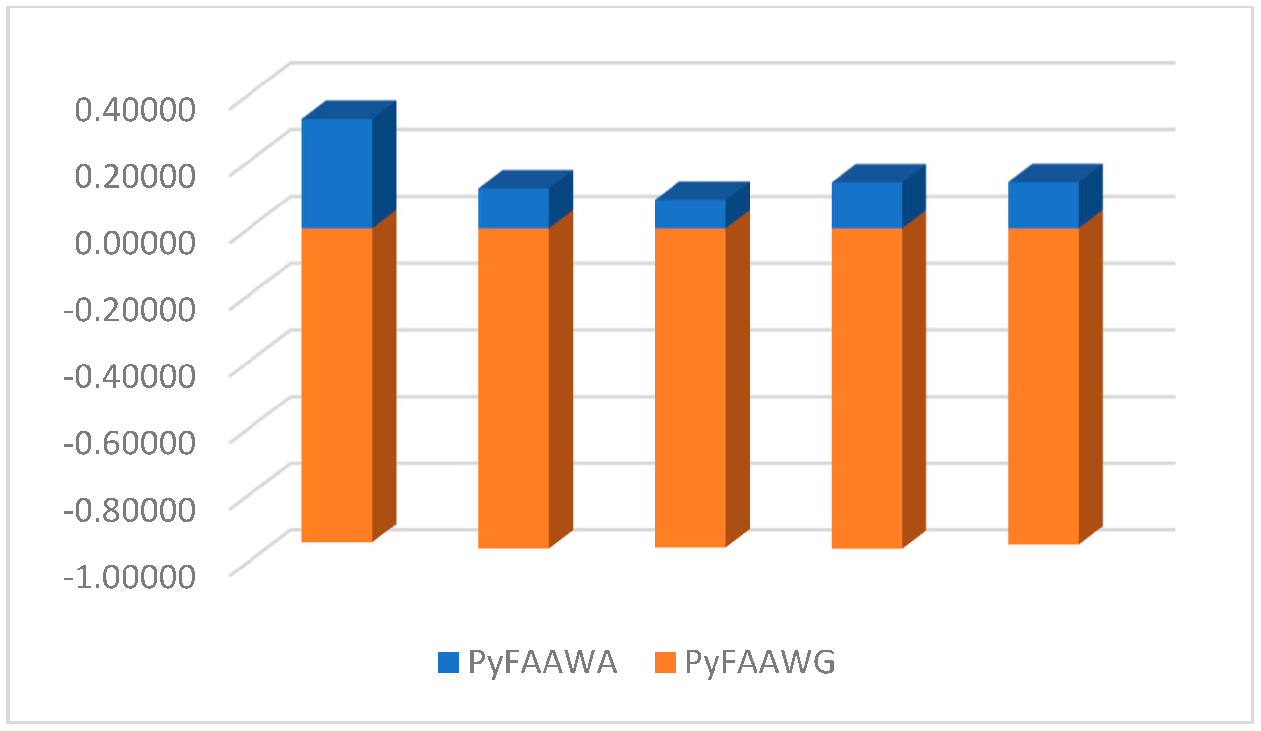
6.3. Influence Study

To find the reliability and consistency of the above example, we utilize the PyF-AA-WG AO under the discussed algorithm. After applying the PyF-AA-WG AO, the results are shown in

Table 2. Ranking and ordering the score values of PyF-AA-WA and PyF-AA-WG operators.

	$\mathit{K}\left({\mathit{𝒴}}_{\mathbf{1}}\right)$	$\mathit{K}\left({\mathit{𝒴}}_{\mathbf{2}}\right)$	$\mathit{K}\left({\mathit{𝒴}}_{\mathbf{3}}\right)$	$\mathit{K}\left({\mathit{𝒴}}_{\mathbf{4}}\right)$	$\mathit{K}\left({\mathit{𝒴}}_{\mathbf{5}}\right)$	Ranking
PYF-AA-WA	$0.32836$	$0.11992$	$0.08606$	$0.13763$	$0.13852$	$G_1\succ G_5\succ G_4\succ G_2\succ G_3$
PYF-AA-WG	$-0.94105$	$-0.95999$	$-0.95670$	$-0.96070$	$-0.94813$	$G_1\succ G_5\succ G_4\succ G_3\succ G_2$

. Furthermore, we analyze these experimental results in graphical interpretation as depicted in Figure 2.

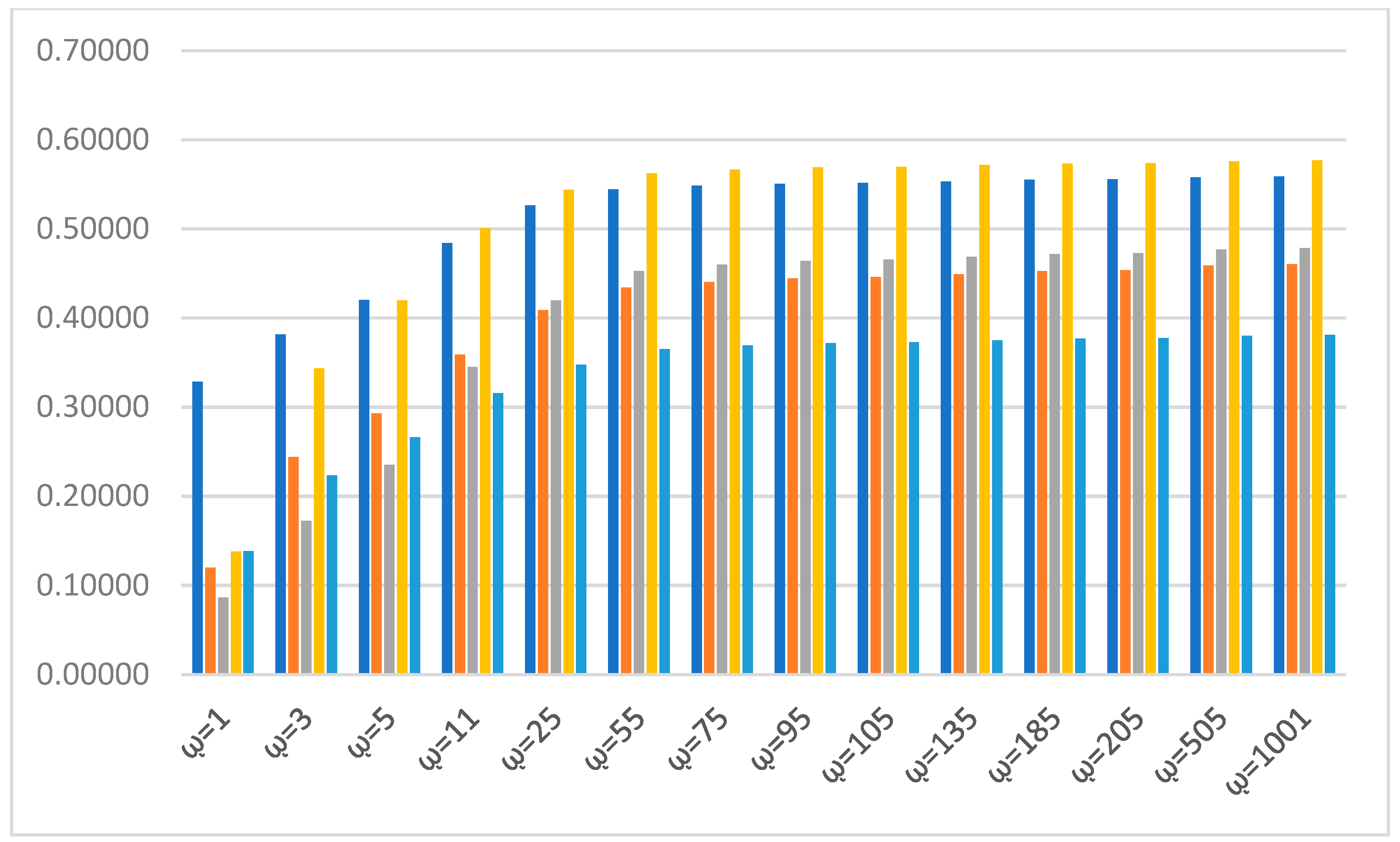
6.4. Impact of Various Parameters on the MADM Techniques

Intending to show the effect of the different extents of the bounds $K$, we take advantage of specific boundary $K$ inside our referenced methods to characterize the other options. The demanding impacts of the other options $G_n\left(n=1,2,3,4,5\right)$ in light of PyF-AA-WA executive are shown in

Table 3. Ranking of Score values by PyF-AA-WA operator for variation of ῳ.

ῳ	$\mathit{K}\left({\mathit{𝒴}}_{\mathbf{1}}\right)$	$\mathit{K}\left({\mathit{𝒴}}_{\mathbf{2}}\right)$	$\mathit{K}\left({\mathit{𝒴}}_{\mathbf{3}}\right)$	$\mathit{K}\left({\mathit{𝒴}}_{\mathbf{4}}\right)$	$\mathit{K}\left({\mathit{𝒴}}_{\mathbf{5}}\right)$	Ordering and Ranking
1	$0.32836$	$0.11992$	$0.08606$	$0.13763$	$0.13852$	$G_1\succ G_5\succ G_4\succ G_2\succ G_3$
3	$0.38169$	$0.24396$	$0.17210$	$0.34337$	$0.22357$	$G_1\succ G_4\succ G_2\succ G_5\succ G_3$
5	$0.41982$	$0.29268$	$0.23515$	$0.41941$	$0.26626$	$G_1\succ G_4\succ G_2\succ G_5\succ G_3$
11	$0.48400$	$0.35861$	$0.34501$	$0.50050$	$0.31572$	$G_4\succ G_1\succ G_2\succ G_3\succ G_5$
25	$0.52601$	$0.40876$	$0.41934$	$0.54389$	$0.34728$	$G_4\succ G_1\succ G_3\succ G_2\succ G_5$
55	$0.54426$	$0.43402$	$0.45231$	$0.56234$	$0.36489$	$G_4\succ G_1\succ G_3\succ G_2\succ G_5$
75	$0.54829$	$0.44026$	$0.45964$	$0.56640$	$0.36929$	$G_4\succ G_1\succ G_3\succ G_2\succ G_5$
95	$0.55061$	$0.44421$	$0.46388$	$0.56874$	$0.37187$	$G_4\succ G_1\succ G_3\succ G_2\succ G_5$
105	$0.55144$	$0.44571$	$0.46539$	$0.56958$	$0.37280$	$G_4\succ G_1\succ G_3\succ G_2\succ G_5$
135	$0.55319$	$0.44905$	$0.46858$	$0.57135$	$0.37475$	$G_4\succ G_1\succ G_3\succ G_2\succ G_5$
185	$0.55485$	$0.45243$	$0.47159$	$0.57301$	$0.37661$	$G_4\succ G_1\succ G_3\succ G_2\succ G_5$
205	$0.55528$	$0.45335$	$0.47238$	$0.57345$	$0.37709$	$G_4\succ G_1\succ G_3\succ G_2\succ G_5$
505	$0.55767$	$0.45849$	$0.47673$	$0.57586$	$0.37977$	$G_4\succ G_1\succ G_3\succ G_2\succ G_5$
1001	$0.55848$	$0.46023$	$0.47820$	$0.57667$	$0.38068$	$G_4\succ G_1\succ G_3\succ G_2\succ G_5$

, and a graphic representation is in Figure 3. It is obvious that when the size of $K$ increases for PyF-AA-WA executive, the score values of the options increments progressively, and yet comparing requesting is something very similar and it is $G_1\succ G_5\succ G_4\succ G_2\succ G_3$. This means that the proposed strategies have the property of intensity, and so the decision makers can choose the appropriate worth as per their capability. In addition, from Figure 3, we reason that the arrangement of the consequences of choices is unclear when the upsides of $K$ have differed in the model, and the predictable positioning results show the dependability of the proposed PyF-AA-WA authority.

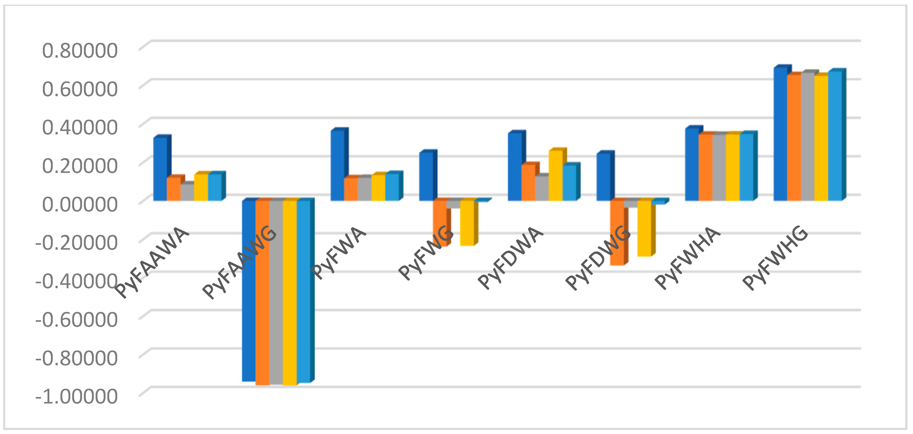
7. Comparative Analysis

In this section, we provide a comparative analysis of our proposed work with the previously existing MADM techniques proposed in Akram et al. [24], Grag [39], Wu et al. [40], Zhang [41], and Garg [42], which are depicted in

Table 4. Comparison of proposed work with some previous existing AOs with ῳ = 1.

	K(Y1)	K(Y2)	K(Y3)	K(Y4)	K(Y5)	Ranking
PyF-AA-WA	0.32836	0.11992	0.08606	0.13763	0.13852	G1 ≻ G5 ≻ G4 ≻ G2 ≻ G3
PyF-AA-WG	−0.94105	−0.95999	−0.95670	−0.96070	−0.94813	G1 ≻ G5 ≻ G4 ≻ G3 ≻ G2
PyF-WA [41]	0.36480	0.11760	0.11986	0.13396	0.14012	G1 ≻ G5 ≻ G4 ≻ G3 ≻ G2
PyF-WG [41]	0.25046	−0.23772	−0.03870	−0.23349	−0.00575	G1 ≻ G5 ≻ G3 ≻ G4 ≻ G2
PyF-WHA [40]	0.376077	0.344281	0.343631	0.345176	0.348061	G1 ≻ G5 ≻ G4 ≻ G3 ≻ G2
PyF-WHG [40]	0.69159	0.65303	0.66563	0.64961	0.67223	G1 ≻ G5 ≻ G3 ≻ G4 ≻ G5
PyD-FWAA [24]	0.35160	0.18683	0.12750	0.26031	0.18395	G1 ≻ G4 ≻ G2 ≻ G5 ≻ G3
PyD-FWGA [24]	0.24558	−0.33607	−0.03446	−0.28931	−0.01921	G1 ≻ G5 ≻ G3 ≻ G4 ≻ G2
PF-WA [39]	Failed
CIF-WA [42]	Failed
IF-AAWA [34]	Failed
IVIF-AAWA [35]	Failed

. From Table 4, it is seen that the AOs presented in [39] and [42] failed the given information by the decision maker in Table 1. The failed reasons for these operators are due to the given information of TG and FG in PyFNs.

Furthermore, the outcomes obtained using the AOs by Wu et al. [40], Zhang [41], and Akram et al. [24] provide different outcomes that are depicted in Table 4. From the above comparison analysis, one can observe the differences in the results obtained by using AA AOs in the frame of PyFSs. The reliability of the results lies in the fact that AA AOs are based on AA-TN, and, hence, are responsible for valid results. The variable parameters associated with AA AOs are also responsible for the reliable results. It is also evident from [31,32] that the AA AOs of IFSs cannot be applied to the information with wider range, and, hence, are limited in nature. All these facts lead to the effectiveness and comprehension of the proposed AA AOs of PyFSs. To illustrate the advantages of our proposed work, a geometrical representation is also depicted in Figure 4.

8. Conclusions

In this paper, we utilized the Aczel–Alsina AOs (AA-AOs) in the framework of PyFSs. We first developed some Aczel–Alsina operators on PyFSs. We then proposed the six types of AA-AOs. These are AA-AOs of PyF-AA-WA, PyF-AA-OWA, PyF-AA-HA, PyF-AA-WG, PyF-AA-OWG, and PyF-AA-HG. Furthermore, we also demonstrated the good properties of these AA-AOs on PyFSs, such as monotonicity, idempotency, and boundedness. Considering the benefits of the PyF-AA-WA and PyF-AA-WG operators, we applied these operators to solve the MADM problem in which a multinational company wants to recruit a position by interviewing applicants with evaluation according to the four attributes of impacts. We also investigate the behaviors of these operators by changing the boundary parameter $ῳ$. We made comparisons between the proposed PyF-AA-WA and PyF-AA-WG operators with the existing operators, such as Akram et al. [24], Grag [39], Wu et al. [40], Zhang [41], and Garg [42], where the proposed operators have better results.

In the near future, we will extend our work in the framework of complex fuzzy graphs [43] by introducing Aczel–Alsina fuzzy graphs. We will further use the AA-TN and AA-TCN in the environment of bipolar fuzzy soft set [44] and complex bipolar fuzzy sets [45] with its applications in MADM and pattern recognition. Furthermore, these AA-TN and AA-TCN will be considered in fuzzy control and interval type-3 fuzzy control systems [46,47], and be extended to the framework of the hesitant pythagorean fuzzy information [48].

References

1. Zadeh, L.A. Fuzzy Sets. Inf. Control 1965, 8, 338–353. [Google Scholar] [CrossRef] [Green Version]
2. Yang, M.-S.; Hung, W.-L.; Cheng, F.-C. Mixed-Variable Fuzzy Clustering Approach to Part Family and Machine Cell Formation for GT Applications. Int. J. Prod. Econ. 2006, 103, 185–198. [Google Scholar] [CrossRef]
3. Yang, M.-S.; Hung, W.-L.; Chang-Chien, S.-J. On a Similarity Measure between LR-Type Fuzzy Numbers and Its Application to Database Acquisition. Int. J. Intell. Syst. 2005, 20, 1001–1016. [Google Scholar] [CrossRef]
4. Atanassov, K.T. Intuitionistic Fuzzy Sets. In Intuitionistic Fuzzy Sets; Springer: Berlin/Heidelberg, Germany, 1999; pp. 1–137. [Google Scholar]
5. Yager, R.R. Pythagorean Fuzzy Subsets. In Proceedings of the 2013 Joint IFSA World Congress and NAFIPS Annual Meeting (IFSA/NAFIPS), Edmonton, AB, Canada, 24–28 June 2013; pp. 57–61. [Google Scholar]
6. Yager, R.R.; Abbasov, A.M. Pythagorean Membership Grades, Complex Numbers, and Decision Making. Int. J. Intell. Syst. 2013, 28, 436–452. [Google Scholar] [CrossRef]
7. Atanassov, K.; Gargov, G. Interval Valued Intuitionistic Fuzzy Sets. Fuzzy Sets Syst. 1989, 31, 343–349. [Google Scholar] [CrossRef]
8. Hussian, Z.; Yang, M.-S. Distance and Similarity Measures of Pythagorean Fuzzy Sets Based on the Hausdorff Metric with Application to Fuzzy TOPSIS. Int. J. Intell. Syst. 2019, 34, 2633–2654. [Google Scholar] [CrossRef]
9. Asif, M.; Akram, M.; Ali, G. Pythagorean Fuzzy Matroids with Application. Symmetry 2020, 12, 423. [Google Scholar] [CrossRef] [Green Version]
10. Menger, K. Statistical Metrics. Proc. Natl. Acad. Sci. USA 1942, 28, 535. [Google Scholar] [CrossRef] [Green Version]
11. Deschrijver, G.; Cornelis, C.; Kerre, E.E. On the representation of intuitionistic fuzzy t-norms and t-conorms. IEEE Trans. Fuzzy Syst. 2004, 12, 45–61. [Google Scholar] [CrossRef]
12. Drossos, C.A. Generalized t-norm structures. Fuzzy Sets Syst. 1999, 104, 53–59. [Google Scholar] [CrossRef]
13. Pap, E.; Bošnjak, Z.; Bošnjak, S. Application of fuzzy sets with different t-norms in the interpretation of portfolio matrices in strategic management. Fuzzy Sets Syst. 2000, 114, 123–131. [Google Scholar] [CrossRef]
14. Stamou, G.B.; Tzafestas, S.G. Resolution of composite fuzzy relation equations based on Archimedean triangular norms. Fuzzy Sets Syst. 2001, 120, 395–407. [Google Scholar] [CrossRef]
15. Wang, S. A fuzzy logic for the revised drastic product t-norm. Soft Comput. 2007, 11, 585–590. [Google Scholar] [CrossRef]
16. Garg, H. Generalized intuitionistic fuzzyinteractive geometric interaction operators using Einstein t-norm and t-conorm and their application to decision making. Comput. Ind. Eng. 2016, 101, 53–69. [Google Scholar] [CrossRef]
17. Ullah, K.; Garg, H.; Gul, Z.; Mahmood, T.; Khan, Q.; Ali, Z. Interval Valued T-Spherical Fuzzy Information Aggregation Based on Dombi t-Norm and Dombi t-Conorm for Multi-Attribute Decision Making Problems. Symmetry 2021, 13, 1053. [Google Scholar] [CrossRef]
18. Xu, Z. Intuitionistic fuzzy aggregation operators. IEEE Trans. Fuzzy Syst. 2007, 15, 1179–1187. [Google Scholar]
19. Rahman, K.; Abdullah, S.; Ghani, F. Some new generalized interval-valued Pythagorean fuzzy aggregation operators using Einstein t-norm and t-conorm. J. Intell. Fuzzy Syst. 2019, 37, 3721–3742. [Google Scholar] [CrossRef]
20. Liu, P.; Wang, P. Some q-rung orthopair fuzzy aggregation operators and their applications to multiple-attribute decision making. Int. J. Intell. Syst. 2018, 33, 259–280. [Google Scholar] [CrossRef]
21. Garg, H. A novel accuracy function under interval-valued Pythagorean fuzzy environment for solving multicriteria decision making problem. J. Intell. Fuzzy Syst. 2016, 31, 529–540. [Google Scholar] [CrossRef]
22. Mahmood, T.; Ullah, K.; Khan, Q.; Jan, N. An Approach toward Decision-Making and Medical Diagnosis Problems Using the Concept of Spherical Fuzzy Sets. Neural Comput. Appl. 2019, 31, 7041–7053. [Google Scholar] [CrossRef]
23. Ali, Z.; Mahmood, T.; Yang, M.S. Complex T-spherical fuzzy aggregation operators with application to multi-attribute decision making. Symmetry 2020, 12, 1311. [Google Scholar] [CrossRef]
24. Akram, M.; Dudek, W.A.; Dar, J.M. Pythagorean Dombi fuzzy aggregation operators with application in multicriteria decision-making. Int. J. Intell. Syst. 2019, 34, 3000–3019. [Google Scholar] [CrossRef]
25. Ashraf, S.; Abdullah, S.; Mahmood, T.; Ghani, F.; Mahmood, T. Spherical fuzzy sets and their applications in multi-attribute decision making problems. J. Intell. Fuzzy Syst. 2019, 36, 2829–2844. [Google Scholar] [CrossRef]
26. Wang, W.; Liu, X. Intuitionistic fuzzy geometric aggregation operators based on Einstein operations. Int. J. Intell. Syst. 2011, 26, 1049–1075. [Google Scholar] [CrossRef]
27. Khan, A.A.; Ashraf, S.; Abdullah, S.; Qiyas, M.; Luo, J.; Khan, S.U. Pythagorean fuzzy Dombi aggregation operators and their application in decision support system. Symmetry 2019, 11, 383. [Google Scholar] [CrossRef] [Green Version]
28. Xing, Y.; Zhang, R.; Wang, J.; Zhu, X. Some new Pythagorean fuzzy Choquet–Frank aggregation operators for multi-attribute decision making. Int. J. Intell. Syst. 2018, 33, 2189–2215. [Google Scholar] [CrossRef]
29. Seikh, M.R.; Mandal, U. Q-rung orthopair fuzzy Frank aggregation operators and its application in multiple attribute decision-making with unknown attribute weights. Granul. Comput. 2022; in press. [Google Scholar] [CrossRef]
30. Mahmood, T.; Waqas, H.M.; Ali, Z.; Ullah, K.; Pamucar, D. Frank aggregation operators and analytic hierarchy process based on interval-valued picture fuzzy sets and their applications. Int. J. Intell. Syst. 2021, 36, 7925–7962. [Google Scholar] [CrossRef]
31. Aczél, J.; Alsina, C. Characterizations of some classes of quasilinear functions with applications to triangular norms and to synthesizing judgements. Aequ. Math. 1982, 25, 313–315. [Google Scholar] [CrossRef]
32. Babu, M.S.; Ahmed, S. Function as the Generator of Parametric T-Norms. Am. J. Appl. Math. 2017, 5, 114–118. [Google Scholar] [CrossRef] [Green Version]
33. Farahbod, F.; Eftekhari, M. Comparison of Different T-Norm Operators in Classification Problems. Int. J. Fuzzy Log. Syst. 2012, 2, 33–39. [Google Scholar] [CrossRef]
34. Senapati, T.; Chen, G.; Yager, R.R. Aczel–Alsina Aggregation Operators and Their Application to Intuitionistic Fuzzy Multiple Attribute Decision Making. Int. J. Intell. Syst. 2022, 37, 1529–1551. [Google Scholar] [CrossRef]
35. Senapati, T.; Chen, G.; Mesiar, R.; Yager, R.R. Novel Aczel–Alsina Operations-Based Interval-Valued Intuitionistic Fuzzy Aggregation Operators and Their Applications in Multiple Attribute Decision-Making Process. Int. J. Intell. Syst. 2022; in press. [Google Scholar] [CrossRef]
36. Hussain, A.; Ullah, K.; Yang, M.-S.; Pamucar, D. Aczel-Alsina Aggregation Operators on T-Spherical Fuzzy (TSF) Information with Application to TSF Multi-Attribute Decision Making. IEEE Access 2022, 10, 26011–26023. [Google Scholar] [CrossRef]
37. Klement, E.P.; Mesiar, R.; Pap, E. Generated Triangular Norms. Kybernetika 2000, 36, 363–377. [Google Scholar]
38. Peng, X.; Yang, Y. Some Results for Pythagorean Fuzzy Sets. Int. J. Intell. Syst. 2015, 30, 1133–1160. [Google Scholar] [CrossRef]
39. Garg, H. Some Picture Fuzzy Aggregation Operators and Their Applications to Multicriteria Decision-Making. Arab. J. Sci. Eng. 2017, 42, 5275–5290. [Google Scholar] [CrossRef]
40. Wu, S.-J.; Wei, G.-W. Pythagorean Fuzzy Hamacher Aggregation Operators and Their Application to Multiple Attribute Decision Making. Int. J. Knowl.-Based Intell. Eng. Syst. 2017, 21, 189–201. [Google Scholar] [CrossRef]
41. Zhang, X. A Novel Approach Based on Similarity Measure for Pythagorean Fuzzy Multiple Criteria Group Decision Making. Int. J. Intell. Syst. 2016, 31, 593–611. [Google Scholar] [CrossRef]
42. Garg, H.; Rani, D. Robust Averaging–Geometric Aggregation Operators for Complex Intuitionistic Fuzzy Sets and Their Applications to MCDM Process. Arab. J. Sci. Eng. 2020, 45, 2017–2033. [Google Scholar] [CrossRef]
43. Hussain, A.; Alsanad, A.; Ullah, K.; Ali, Z.; Jamil, M.K.; Mosleh, M.A. Investigating the Short-Circuit Problem Using the Planarity Index of Complex q-Rung Orthopair Fuzzy Planar Graphs. Complexity 2021, 2021, 8295997. [Google Scholar] [CrossRef]
44. Mahmood, T. A Novel Approach towards Bipolar Soft Sets and Their Applications. J. Math. 2020, 2020, 4690808. [Google Scholar] [CrossRef]
45. Nasir, A.; Jan, N.; Yang, M.S.; Pamucar, D.; Marinkovic, D.; Khan, S.U. Security Risks to Petroleum Industry: An Innovative Modeling Technique Based on Novel Concepts of Complex Bipolar Fuzzy Information. Mathematics 2022, 10, 1067. [Google Scholar] [CrossRef]
46. Mosavi, A.; Qasem, S.N.; Shokri, M.; Band, S.S.; Mohammadzadeh, A. Fractional-Order Fuzzy Control Approach for Photovoltaic/Battery Systems under Unknown Dynamics, Variable Irradiation and Temperature. Electronics 2020, 9, 1455. [Google Scholar] [CrossRef]
47. Liu, Z.; Mohammadzadeh, A.; Turabieh, H.; Mafarja, M.; Band, S.S.; Mosavi, A. A New Online Learned Interval Type-3 Fuzzy Control System for Solar Energy Management Systems. IEEE Access 2021, 9, 10498–10508. [Google Scholar] [CrossRef]
48. Akram, M.; Luqman, A.; Alcantud, J.C.R. An Integrated ELECTRE-I Approach for Risk Evaluation with Hesitant Pythagorean Fuzzy Information. Expert Syst. Appl. 2022, 200, 116945. [Google Scholar] [CrossRef]
Figure 1. Graphical representation of IFSs and PyFSs.
Symmetry 14 00940 g001
Figure 2. Graphical representation of PyF-AA-WA and PyF-AA-WG operators.
Symmetry 14 00940 g002
Figure 3. Score values of the PyF-AA-WA operator for different ῳ.
Symmetry 14 00940 g003
Figure 4. Comparison of proposed work with previous existing AOs.
Symmetry 14 00940 g004