
An Improved EDAS Method for the Multi-Attribute Decision Making Based on the Dynamic Expectation Level of Decision Makers


1
Department of Mathematics, Hunan University of Science and Technology, Xiangtan 411201, China
2
Department of Mathematics, Central South of University, Changsha 410081, China
*
Author to whom correspondence should be addressed.
Symmetry 2022, 14(5), 979; https://0-doi-org.brum.beds.ac.uk/10.3390/sym14050979
Submission received: 13 April 2022
/
Revised: 2 May 2022
/
Accepted: 5 May 2022
/
Published: 10 May 2022
(This article belongs to the Special Issue Fuzzy Set Theory and Uncertainty Theory)
Abstract
:The improved evaluation based on the distance from average solution (EDAS) of the interval-valued intuitionistic trapezoidal fuzzy set is proposed. At first, we propose a new distance between interval-valued intuitionistic trapezoidal fuzzy numbers according to their interval endpoints and centroid point, and its properties are also discussed. Furthermore, we apply the proposed distance measure to calculate the expectation level of the emergency plan, and the optimal dynamic expectation level of the emergency plan is obtained by solving the programming model. Then, we improve the EDAS method based on the dynamic expectation level of the decision makers and apply it to calculate the optimal emergency plan. Finally, a numerical example about flood disaster rescue is given to verify the feasibility and effectiveness of the proposed method, which is also compared with the existing methods.
1. Introduction
In recent years, torrential rain, typhoons and other emergencies have brought great risk to the safety of human life and property. For example, the Henan province in China suffered a rare torrential rain in July 2021, and the disaster affected 14.786 million people, causing an economic loss of CNY 120.06 billion [1]. Emergency management departments carry out risk management for disaster events, which is beneficial to early scientific warning and emergency rescue for the disaster.
The uncertainty of emergency decisions requires the decision maker to adjust the emergency plan dynamically. Generally, the emergency plan is evaluated from the following aspects: the representation of the emergency plan and the choice of decision-making method. Since the fuzzy set was proposed by Zadeh L.A. [2], it has been paid much attention and popularized by many researchers, as it provides an effective tool for dealing with the uncertain information in emergency decision making. For example, Guo et al. [3] applied the variable fuzzy set and set pair analysis to evaluate flood disaster risk. Wu et al. [4] discussed the emergency rescue of flood disaster by using the linguistic intuitionistic fuzzy set and TOPSIS method. He [5] applied Dombi hesitant fuzzy set to deal with the problem of typhoon disaster risk. Many studies on the application of uncertain sets in emergency decision making are summarized in Table 1. The uncertain sets mentioned in Table 1 are all numerical sets. However, the linguistic term set or interval-valued fuzzy set are more suitable to represent the uncertain information. For example, Peng et al. [6] applied the interval-valued Pythagorean fuzzy set to describe the uncertain information in mineral emergency safety. How to deal with the uncertainty in emergency decision-making has become an important topic.
The choice of emergency decision-making methods is also very important. Ren et al. [13] applied the TOPSIS method and prospect theory to construct the optimal emergency plan for explosions. The essence of the TOPSIS method is to find the alternative closest to the optimal alternative and farthest from the worst alternative, but it does not consider the psychological factors of decision makers. In fact, the psychological factors of decision makers also affect the efficiency of emergency plan. For example, the TODIM method takes into account the psychological factors of decision makers. Liang et al. [14] extended the TODIM method into the hesitant fuzzy linguistic environment and applied it to solve the problem of mineral emergency. Ding et al. [15] proposed the dynamic TODIM method under the probabilistic hesitant fuzzy set and applied it to solve fire emergency rescue. In fact, the attributes in multi-attribute decision making problems affect each other. In order to eliminate the interaction between attributes, Keshavarz et al. [16] proposed the EDAS (Evaluation based on distance from average solution) method to deal with the classification of conflict criteria. Keshavarz et al. [17] continued to propose the dynamic EDAS method in a changing emergency decision environment. In fact, EDAS applies the average solution to appraise the alternatives, where two measures are called PDA (positive distance from average) and NDA (Negative distance from average). In practical decision making problems, the value of two measures is not only related to the average solution but also related to its standard deviation.
Motivated by this, we propose a new EDAS method based on the expectation level of decision makers and apply it to emergency decision making. The contributions and advantages of the paper are given as follows.
(1) A new distance measure is defined based on the interval endpoints and centroid point of interval-valued intuitionistic trapezoidal fuzzy numbers.
(2) We apply the programming model to calculate the dynamic expectation level of decision makers, which can provide a real-time reference point for the emergency plan and improve the efficiency of the emergency plan.
(3) An improved EDAS method is proposed based on the prospect theory; the corresponding and not only consider the distance to the average but also its standard deviation.
The rest of the paper is organized as follows: In Section 2, some basic concepts of interval-valued intuitionistic trapezoidal fuzzy number, prospect theory and EDAS method are reviewed. In Section 3, we first propose a new distance measure between interval-valued intuitionistic trapezoidal fuzzy numbers, and the dynamic expectation level of decision makers is also obtained by solving the programming model. In Section 4, an improved EDAS method based on the dynamic expectation level of the decision makers is proposed. In Section 5, we apply the proposed method to the numerical example of flood disaster rescue, which is also compared with the existing methods. In Section 6, we summarize the paper and put forward the research direction in the future.
2. Preliminaries
In this section, we briefly review some basic concepts of interval-valued intuitionistic trapezoidal fuzzy number, prospect theory and EDAS method.
2.1. Interval-Valued Intuitionistic Trapezoidal Fuzzy Number
In this sub-section, the concept of interval-valued intuitionistic trapezoidal fuzzy numbers and its weighted arithmetic average (WAA) operator are presented as follows.
Definition 1.
([18]) Let be a universe of discourse, a collection of interval-valued intuitionistic trapezoidal fuzzy numbers on X is defined as
where , and represent the membership degree and non-membership degree, respectively, and they satisfy with .
The weighted arithmetic average operator of interval-valued intuitionistic trapezoidal fuzzy numbers is given as follows.
Definition 2.
([19]) Let be a collection of interval-valued intuitionistic trapezoidal fuzzy numbers, if is the corresponding weight vector of , satisfying with , then the weighted arithmetic average operator of interval-valued intuitionistic trapezoidal fuzzy numbers is defined as
2.2. Prospect Theory
The decision-making process is divided into two stages based on the prospect theory: the first stage is the occurrence of random events; and the second stage is the evaluation of the random events.
Suppose the evaluation information of the alternative A is x, if the reference point is , then the value function of the alternative A is given as follows ([20]):
where the parameters and represent the decision makers’ attitudes in the gain and loss, respectively. represents the loss-avoidance coefficient of decision makers. For example, indicates the decision makers are more sensitive to loss.
2.3. Evaluation Based on Distance from Average Solution (EDAS)
The EDAS method proposed by Keshavarz [16], which is applied to rank the alternatives. The calculation process is summarized as follows:
(1) Determine the average solution based on the evaluation information under all attributes.
(2) Calculate the positive distance from average and the negative distance from average , respectively,
If the attribute j is beneficial, then and ;
If the attribute j is cost, then and , where represents the average value under the attribute j.
(3) Aggregate the and for all emergency plans, then
where is the weight of attribute j.
(4) Calculate the appraisal score for all emergency plans, where . Furthermore, we rank the emergency plan in descending order of the value of .
3. The Dynamic Expectation Level of the Emergency Plan Based on the Programming Model
In the process of emergency decision making, the decision makers often show different psychological characteristics. In order to obtain the dynamic expectation level of the emergency plan, we first propose a new distance measure between the interval-valued intuitionistic trapezoidal fuzzy numbers.
3.1. A New Distance between Interval-Valued Intuitionistic Trapezoidal Fuzzy Numbers
Wan [19] defined the normalized Hamming distance between interval-valued intuitionistic trapezoidal fuzzy numbers as follows.
Definition 3.
([19]) Let and be two interval-valued intuitionistic trapezoidal fuzzy numbers, the normalized Hamming distance between and is denoted as , which is given by
The above distance measure only considered the interval endpoints of interval-valued intuitionistic trapezoidal fuzzy numbers. Its value is not only related to the interval endpoints but also related to the points whose two interval endpoints are symmetric. Its irrationality can be seen from the Example 1.
Example 1.
Let and be two interval-valued intuitionistic trapezoidal fuzzy numbers, then .
Although , the two interval-valued intuitionistic trapezoidal fuzzy numbers are not equal, which is unreasonable. Considering that the distance measure between interval-valued intuitionistic trapezoidal fuzzy numbers is not only related to the endpoints of the interval but also related to its centroid point, we should define a new distance. Firstly, we introduce the concept of centroid point of interval-valued intuitionistic trapezoidal fuzzy number on the basis of the idea of symmetric interval set.
Definition 4.
([21]) Let be an interval-valued intuitionistic trapezoidal fuzzy number, the centroid point of H is defined as
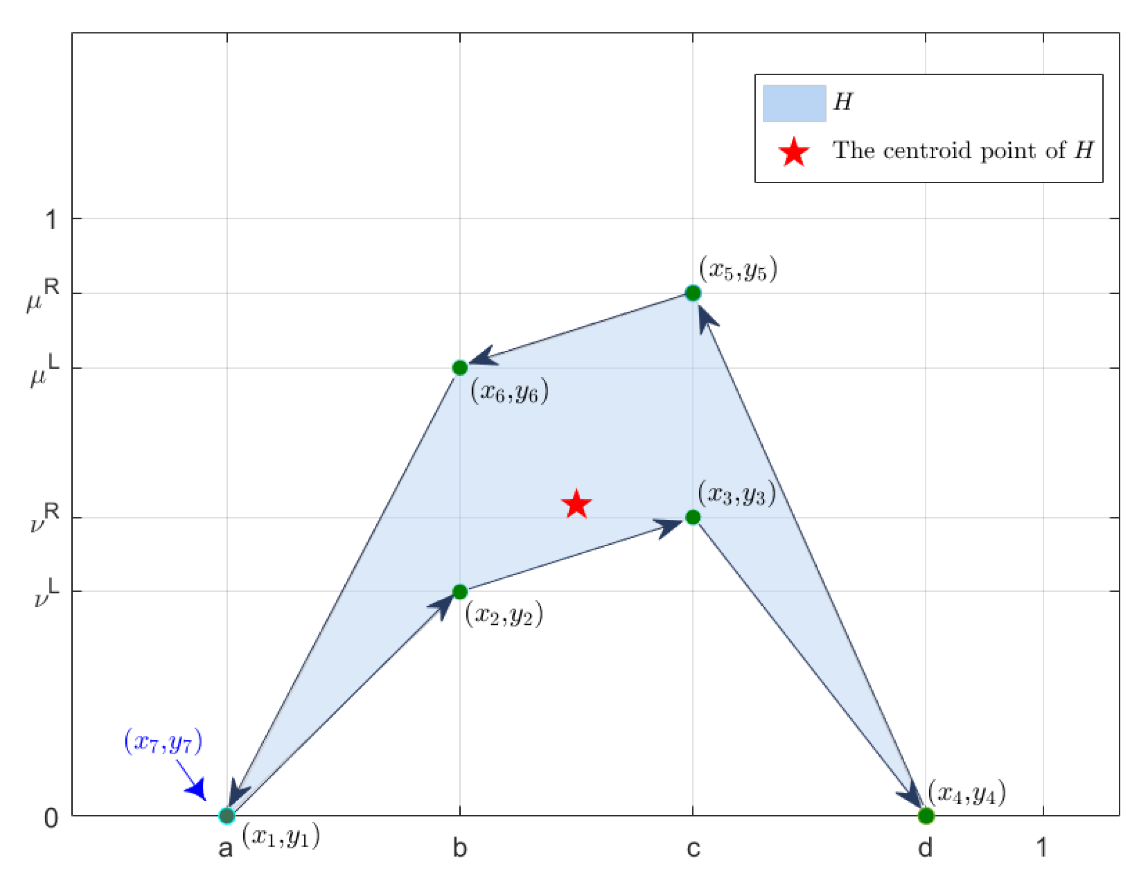
where , , , , , . Furthermore, , then the geometric representation of interval-valued intuitionistic trapezoidal fuzzy number H is given in Figure 1.
Next, we propose a new distance measure between interval-valued intuitionistic trapezoidal fuzzy numbers based on the interval endpoints and centroid point.
Definition 5.
Let and be two interval-valued intuitionistic trapezoidal fuzzy numbers, and are the centroid point of and , respectively, the distance measure is defined as
where and represent the preference for the membership degree and the centroid point, respectively. If , which means that we ignore the influence of centroid point, the distance measure is reduced to the normalized Hamming distance measure.
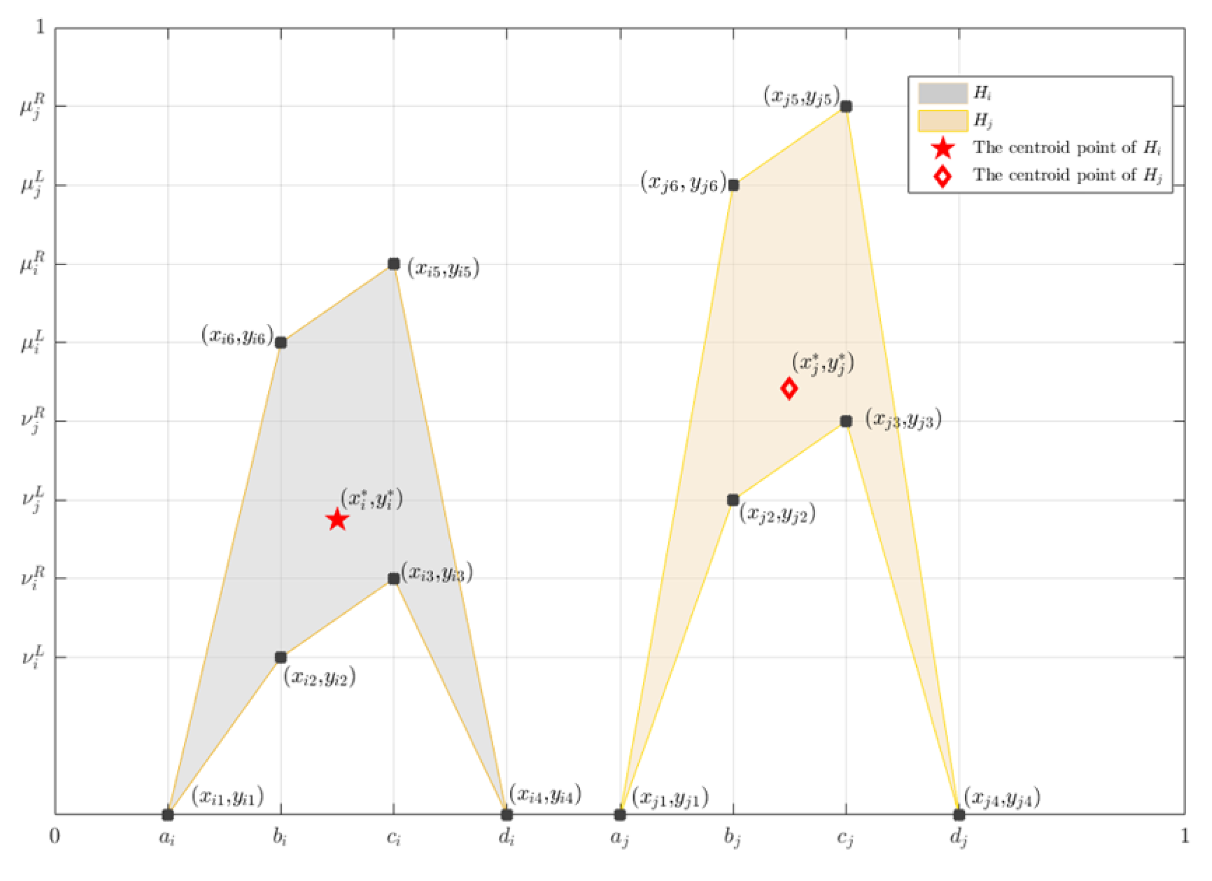
The corresponding geometric representations of and are given in Figure 2.
Theorem 1.
Let and be two interval-valued intuitionistic trapezoidal fuzzy numbers, the distance measure satisfies the following properties:
;
;
if and only if ;
For a given interval-valued intuitionistic trapezoidal fuzzy number , then .
Proof. (1)
If , then
Because , then
So is obtained.
(2) If
and
then is obtained.
If , then
So we have .
Furthermore, if , then
If , and ,
and
Thus is obtained.
□
Remark 1.
The difference between the distance measure and dissimilarity measure is that for the give uncertain sets and C, if , then the distance measure satisfies the condition , but the dissimilarity measure satisfies the condition .
The following Example 2 can illustrate the difference between the distance measure and the dissimilarity measure.
Example 2.
Let be a given set, , and are the three picture fuzzy sets, we need to recognize whether the belongs to or .
For the given picture fuzzy sets and , the dissimilarity measure , then and . According to the calculation results, we cannot decide whether belongs to or . For the given distance measure , and . At this time, we know that belongs to .
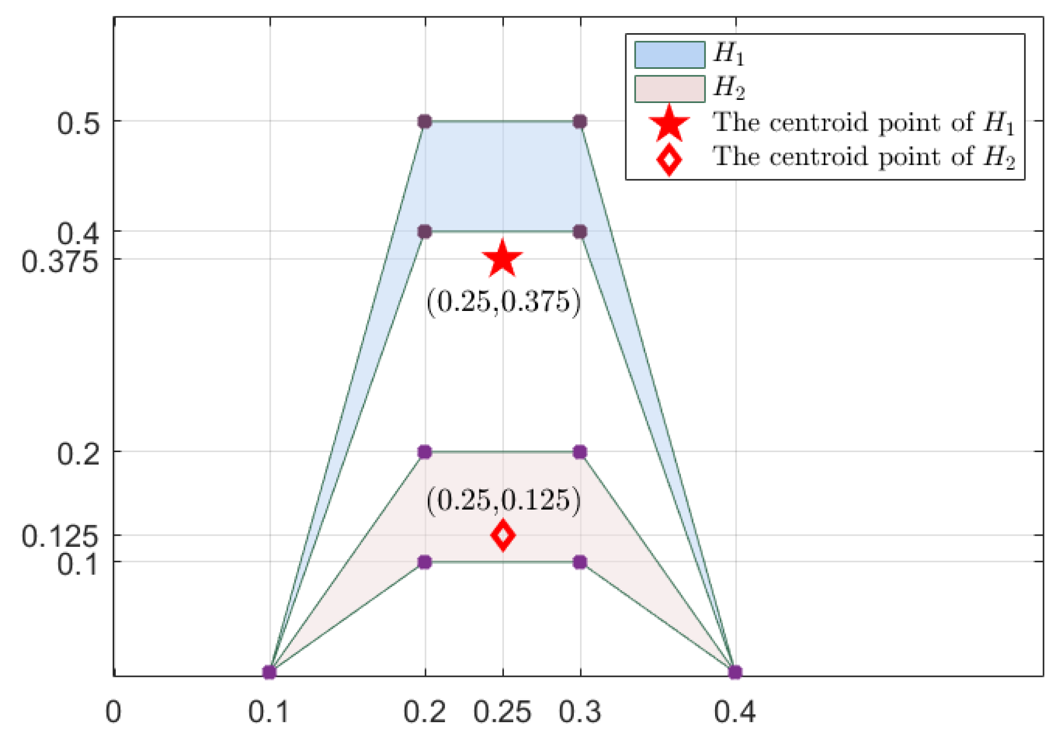
Example 3.(Continued to Example 1) Let and be two interval-valued intuitionistic trapezoidal fuzzy numbers, the centroid points of and are and , respectively. If , the distance measure . The geometric representations of and are given in Figure 3.
3.2. The Dynamic Expectation Level of the Emergency Plan
The development of emergency decision has the characteristics of randomness and dynamics, which requires the decision makers to adjust the emergency plan dynamically. Actually, the decision maker has an expectation level for the emergency decision-making plan. In order to describe the expectation level of the decision makers, we give its definition in the following.
Definition 6.
In the stage , an expectation level of the emergency plan under the attribute j is defined as
where represents the distance between the emergency plan and the positive ideal plan under the attribute j (the distance between the emergency plan and the negative ideal plan under the attribute j ).
Example 4.
The four emergency plans in the stage are represented by the interval-valued intuitionistic trapezoidal fuzzy numbers , , and , respectively. The corresponding positive ideal plan and negative ideal plan are and , respectively, then and . We get the expectation level of the emergency plans as follows: , , and . According to the calculation results, the best emergency plan is .
In the emergency decision making, the optimal emergency plan are dynamic. In order to obtain the optimal emergency plan in stage , we propose a programming model to calculate the maximum expectation level of emergency plan under each attribute. Here, the weights of each attribute are completely unknown.
Because , we normalize it by the formula .
For the given stage , assume is the normalized expectation level of the emergency plan under the attribute , is the weight of attribute , then represents the comprehensive expectation level of emergency plan in stage . The main idea about solving the dynamic expectation level of emergency plan is given as follows.
According to the maximum expectation level principle, we can obtain the optimal expectation level in stage .
In stage , the attribute weight is used to aggregate the expectation level , which can reach the maximum expected level in the whole.
In stage , the optimal expectation level of the emergency plan under the attribute can be obtained by .
So the programming model of the dynamic expectation level of the emergency plan is defined as:
where represents the expectation level value of the emergency plan in stage , the reason why is that the weights are completely unknown.
By solving the programming model, we can obtain the optimal attribute weight and the optimal expectation level .
4. An Improved EDAS Method Based on the Dynamic Expectation Level of the Emergency Plan
In this section, we propose an improved EDAS method for the emergency plan, the dynamic expectation level of the decision maker is also included.
The EDAS is a decision-making method based on the distance from the average, its key points are the positive distance to average (PDA) and negative distance to average (NDA). In fact, the value is not only related to the distance from the average solution but also related to its standard deviation. The standard deviation of the emergency plan can measure the degree of deviation from the average solution.
In the following, we propose an improved EDAS method based on the dynamic expectation level of the emergency plan as follows.
In the actual decision making process, the decision makers often apply the linguistic variables to describe the evaluation value. According to Liu [22], the linguistic variables are transformed into interval-valued intuitionistic trapezoidal fuzzy numbers (IITrFNs), which is given in Table 2.
In stage , the expert evaluates the emergency plan. The transformed evaluation information of the emergency plan under the attribute can be represented as an interval-valued intuitionistic trapezoidal fuzzy decision matrix , which is expressed by
where are the interval-valued intuitionistic trapezoidal fuzzy numbers, the weight of decision maker is in stage . The specific algorithm process is given as follows:
Step 1. Aggregate the interval-valued intuitionistic trapezoidal fuzzy decision matrix , which is calculated by .
Step 2. Normalize the expectation level of emergency plan based on the aggregation matrix , we have
where , and .
Step 3. Calculate the dynamic expectation level of emergency plan based on the prospect theory, the calculation process is given as follows.
Firstly, we apply the programming model to calculate the optimal attribute weight , and the optimal expectation level of the emergency plan is also expressed by .
Secondly, the value function of emergency plan in stage is defined as
where , and represents the loss avoidance of decision makers.
Step 4. According to the distance from average solution and the standard deviation of emergency plan, we calculate the improved positive distance to average and the improved negative distance to average , respectively.
If the attribute j is beneficial, the and of the alternative in stage are given by
If the attribute j is cost, the and of the alternative are given by
where represents the average solution of the emergency plan under the attribute , and represent the preference for the average and deviation, respectively.
If , the and are reduced to and , respectively. Here, we assume .
Step 5. Aggregate and of the emergency plan, which are obtained as follows:
where is obtained in Step 3.
Step 6. Calculate the integrative appraisal score of the emergency plan , which is given by
Step 7. Rank the emergency plan in descending order of the value of , the larger value of is, the better emergency plan is.
At the end of this section, we give the importance of improving EDAS method through a numerical example.
Example 5.
In the emergency rescue of flood diaster, the expert evaluates the emergency plans from the attributes ; the evaluation information matrix is shown in Table 3.
We apply the original EDAS method and the improved EDAS method to calculate the positive distance from average solution and the negative distance from average solution, respectively. The calculation results are given in Table 4 and Table 5.
Furthermore, we calculate the integrative appraisal score of the alternative , which is given in Table 6.
As can be seen from the Table 6, the value of the in the original EDAS method are all equal to 0.5, the optimal emergency plan cannot be determined at this time. However, the improved EDAS method consider the deviation from the mean value of the emergency plans, which can overcome the shortcomings of the original EDAS method.
5. Numerical Example
In this section, we apply the proposed method to calculate the optimal emergency plan of the flood disaster rescue, which is also compared with the existing methods.
5.1. An Emergency Rescue of Flood Disaster
China is one of the countries that suffered the most natural disasters in the world. In recent years, natural disasters such as floods, droughts and typhoons show a trend of higher frequency and stronger loss; thus, emergency decision making during natural disasters is a research hotspots. However, the uncertainty in natural disasters affect the efficiency of emergency plans. In the following, we apply the improved EDAS method to solve the problem of flood disaster rescue.
In the emergency rescue during a flood disaster (adapted from Liu [22]), the description of emergency plan is given in Table 7, and the real-time description of the environment in different stages is given in Table 8. The decision makers evaluate the emergency plan from the following five attributes: feasibility (), integrity (), operability (), timeliness () and economy (). In stage , the corresponding evaluation of the emergency plan under the attribute is given in Table 9, and the relationship between the interval-valued intuitionistic trapezoidal fuzzy numbers and the linguistic variables is given in Table 2 in Section 4. It is assumed that the weight of three decision makers is .
According to Table 2, the linguistic evaluation information of emergency plans are transformed into the interval-valued intuitionistic trapezoidal fuzzy numbers, which are obtained in Table 10, Table 11 and Table 12, respectively.
In the following, the calculation process of the numerical example is given as follows (Here ):
Step 1. Apply the Formula (1) to aggregate the evaluation information, the aggregated result is obtained in Table 13.
Step 2. Apply the Formula (8) to calculate the normalized expectation level of emergency plan in stage , the results are given in Table 14.
Step 3. By solving the programming model (7), the optimal attribute weights are given in Table 15. Furthermore, for the given stage , we apply the formula to calculate the optimal expectation levels of emergency plan under each attribute, which are obtained in Table 16.
According to the conclusion obtained in [23], if and , the decision results are more consistent with the empirical results. So we assume that and in the paper, and the value of emergency plan in the stage are obtained in Table 17.
Step 4. Because all attributes are beneficial, we apply (10) to calculate the improved positive distance to average solution and the improved negative distance to average solution , respectively, which are obtained in Table 18 and Table 19.
Step 5. Apply (12) to aggregate and of the emergency plan, which are denoted as and in Table 20, respectively.
Step 6. Calculate the integrative appraisal score , which is also obtained in Table 20.
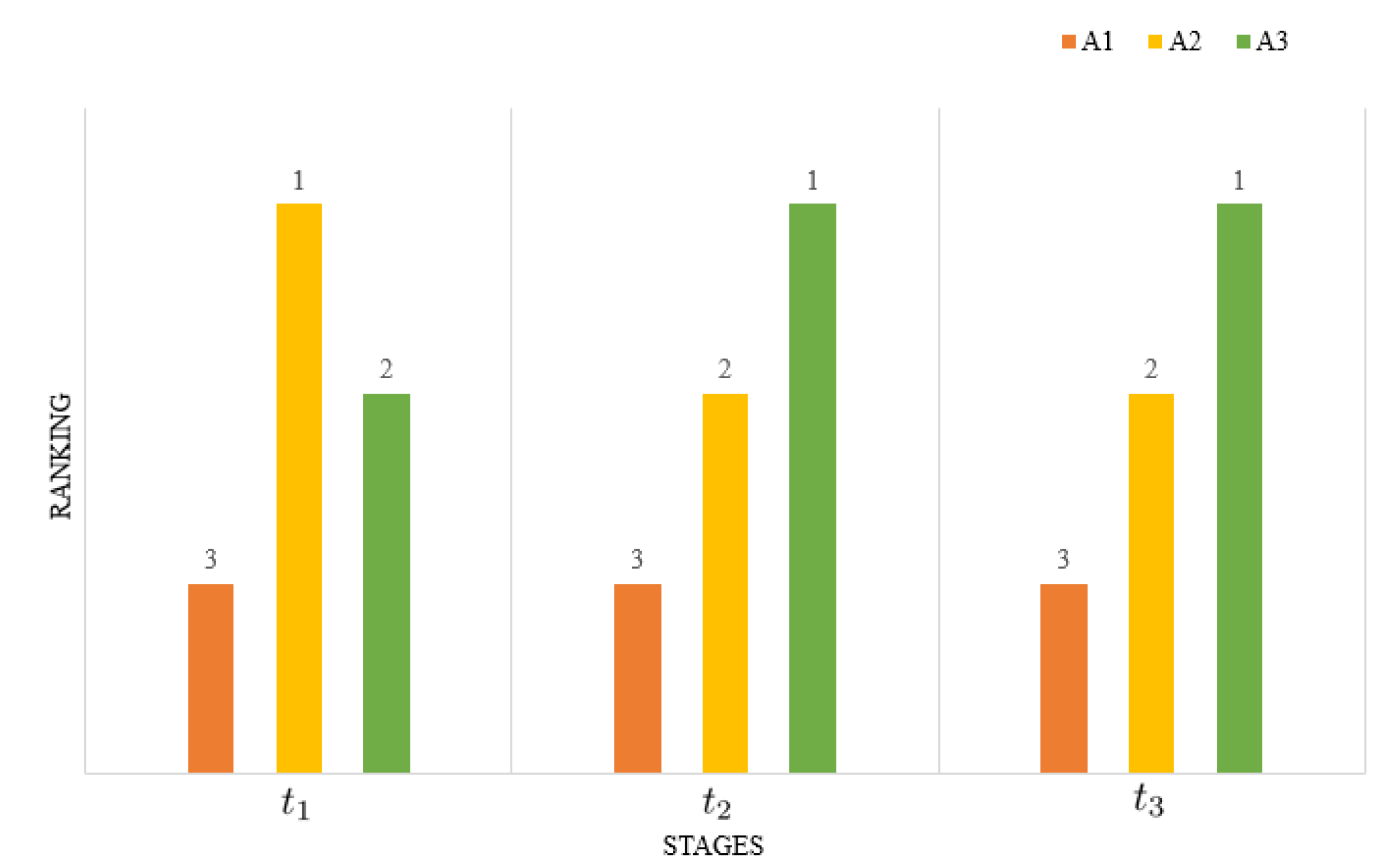
Step 7. In stage , the ranking of emergency plan is . In stage and stage , the ranking of emergency plans are all . And the ranking results of the emergency plan is shown in Figure 4.
According to the calculation results for the given stage the emergency plan is to close one side of the road and keep the traffic moving, we should rescue with small machines. In stage and stage , the emergency rescue plan is to close all traffic lanes except the emergency vehicles, and we should rescue with large machines.
5.2. Comparison with the Existing Methods
In order to verify the feasibility of the improved EDAS method, the calculation results of the proposed method are compared with the methods in Wan [19], Liu [22] and Li et al. [24]. The calculation results and the comparison results are shown in Table 21 and Table 22, respectively.
As can be seen from Table 21, the ranking result obtained by the improved EDAS method is same as the existing methods, which illustrate the rationality of the proposed method.
Furthermore, in order to discuss the sensitivity of the calculation results of the proposed method, we assume that the attribute weights are all equal, and the corresponding comparison results are shown in Table 23.
As can be seen from Table 23, although the weights of attributes are changed, the ranking results of the emergency plan are same as the proposed method, which shows the stability of the improved EDAS method.
In particular, the advantages of the proposed method are given as follows:
Wan [19] and Liu [22] do not consider the expectation level of decision makers for the emergency plan, the proposed method in the paper makes up for their shortcomings, which is beneficial to improve the efficiency of the emergency plan. For example, in the first stage of emergency decision making, the feasibility and timeliness of the emergency plan should be given in priority. In the second stage, the emergency plan gives priority to its feasibility and integrity. In the third stage, the dynamic adjustment of emergency plan should be considered for all attributes. However, there is no justification for the alternatives and attributes in Wan [19] and Liu [22].
The calculation process in this paper is simpler than that in Li et al. [24]. Furthermore, the proposed emergency decision-making method is dynamic, which is more consistent with reality.
The improved EDAS method not only considers the distance to average solution but also considers its standard deviation.
6. Conclusions
An improved evaluation based on distance from average solution for the interval-valued intuitionistic trapezoidal fuzzy numbers is proposed, the paper has made some contributions in the following aspects.
The proposed method in the paper considers the decision maker’s expectation level of the emergency plan, which can better deal with the dynamic development of emergency plan.
The new distance measure between interval-valued intuitionistic trapezoidal fuzzy numbers is applied to calculate the expected level of decision makers, and the emergency plan obtained by the improved EDAS method is more consistent with the real situation.
But the paper also has some limitations, for example, it does not consider the consistency of decision makers’ information. It can also consider the emergency decision-making plan of multi-source information fusion.
In the future, we will continue to study the proposed method from the following aspects: the information consistency of multiple decision makers and the optimal consistency adjustment of evaluation information in the decision-making process. Furthermore, the EDAS method under the continuous fuzzy information and multi-source information will also be considered. In addition, we will also apply the proposed method to investment decision making, the evaluation of engineering projects, group decision making in emergency fields and so on.
Author Contributions
D.P. contributed to the writing of the manuscript. J.W. contributed to the numerical calculation and chart drawing of the manuscript. D.L. and Z.L. performed the analysis with constructive discussions. All authors have read and agreed to the published version of the manuscript.
Funding
The study is fully supported by the National Nature Science Foundation of China (No: 72171080), by the National Nature Science Foundation of China (No: 12071487), by the National Nature Science Foundation of Hunan (No: 2021JJ30285), by the key project of Hunan Provincial Department of Education (No: 21A0302), by the Postgraduate Scientific Research Innovation Project of Hunan Province (No: CX20201003), by Hunan Province College Students’ Science and Technology Innovation and Entrepreneurship Project (No: 2021RC1012).
Institutional Review Board Statement
Not applicable.
Informed Consent Statement
Not applicable.
Data Availability Statement
Not applicable.
Conflicts of Interest
The authors declare no conflict of interests regarding the publication for the paper.
References
- Liu, N.; Jin, W.; Zhang, P.; Zhang, Y.; Wang, G. Analysis of impact characteristics and suggestions on disaster reduction for “7.20” extreme rainstorm disasters in Henan Province 2021. China Flood Drought Manag. 2022, 32, 31–37. [Google Scholar] [CrossRef]
- Zadeh, L.A. Fuzzy sets. Inf. Control 1965, 8, 338–353. [Google Scholar] [CrossRef] [Green Version]
- Guo, E.; Zhang, J.; Ren, X.; Zhang, Q.; Sun, Z. Integrated risk assessment of flood disaster based on improved set pair analysis and the variable fuzzy set theory in central Liaoning Province, China. Nat. Hazards 2014, 74, 947–965. [Google Scholar] [CrossRef]
- Wu, H.; Wang, J.W.; Liu, S.; Yang, T. Research on decision–making of emergency plan for waterlogging disaster in subway station project based on linguistic intuitionistic fuzzy set and TOPSIS. Math. Biosci. Eng. 2020, 17, 4825–4851. [Google Scholar] [CrossRef] [PubMed]
- He, X. Typhoon disaster assessment based on Dombi hesitant fuzzy information aggregation operators. Nat. Hazards 2018, 90, 1153–1175. [Google Scholar] [CrossRef]
- Peng, X.; Li, W. Algorithms for interval–valued pythagorean fuzzy sets in emergency decision making based on multiparametric similarity measures and WDBA. IEEE Access 2019, 7, 7419–7441. [Google Scholar] [CrossRef]
- Liu, X.; Wang, Z.; Zhang, S. A new methodology for hesitant fuzzy emergency decision making with unknown weight information. Complexity 2018, 2018, 1–12. [Google Scholar] [CrossRef]
- Ashraf, S.; Abdullah, S.; Almagrabi, A.O. A new emergency response of spherical intelligent fuzzy decision process to diagnose of COVID19. Soft Comput. 2020, 2020, 29. [Google Scholar] [CrossRef]
- Ding, X.F.; Zhang, L.; Liu, H.C. Emergency decision making with extended axiomatic design approach under picture fuzzy environment. Expert Syst. 2020, 37, e12482. [Google Scholar] [CrossRef]
- Li, H.; Guo, J.Y.; Yazdi, M.; Nedjati, A.; Adesina, K.A. Supportive emergency decision–making model towards sustainable development with fuzzy expert system. Neural Comput. Appl. 2021, 33, 15619–15637. [Google Scholar] [CrossRef]
- Ding, X.; Li, Q. Optimal risk allocation in alliance infrastructure projects: A social preference perspective. Front. Eng. Manag. 2020, 2020, 1–11. [Google Scholar] [CrossRef]
- Kang, L.; Li, H.; Li, C.; Xiao, N.; Sun, H.; Buhigiro, N. Risk warning technologies and emergency response mechanisms in Sichuan–Tibet Railway construction. Front. Eng. Manag. 2021, 8, 582–594. [Google Scholar] [CrossRef]
- Ren, P.; Xu, Z.; Hao, Z. Hesitant fuzzy thermodynamic method for emergency decision making based on prospect theory. IEEE Trans. Cybern. 2016, 47, 2531–2543. [Google Scholar] [CrossRef] [PubMed]
- Liang, Y.; Tu, Y.; Ju, Y.; Shen, W. A multi-granularity proportional hesitant fuzzy linguistic TODIM method and its application to emergency decision making. Int. J. Disaster Risk Reduct. 2019, 36, 101081. [Google Scholar] [CrossRef]
- Ding, Q.; Wang, Y.M.; Goh, M. TODIM dynamic emergency decision–making method based on hybrid weighted distance under probabilistic hesitant fuzzy information. Int. J. Fuzzy Syst. 2021, 23, 474–491. [Google Scholar] [CrossRef]
- Keshavarz Ghorabaee, M.; Zavadskas, E.K.; Olfat, L.; Turskis, Z. Multi-criteria inventory classification using a new method of evaluation based on distance from average solution (EDAS). Informatica 2015, 26, 435–451. [Google Scholar] [CrossRef]
- Keshavarz Ghorabaee, M.; Amiri, M.; Zavadskas, E.K.; Turskis, Z.; Antucheviciene, J. A dynamic fuzzy approach based on the EDAS method for multi–criteria subcontractor evaluation. Information 2018, 9, 68–82. [Google Scholar] [CrossRef] [Green Version]
- Wang, J. Overview on fuzzy multi–criteria decision–making approach. Control Decis. 2008, 23, 601–607. [Google Scholar]
- Wan, S. Multi-attribute decision making method based on interval intuitionistic trapezoidal fuzzy number. Control Decis. 2012, 27, 455–458. [Google Scholar]
- Tversky, A.; Kahneman, D. Advances in prospect theory: Cumulative representation of uncertainty. J. Risk Uncertain. 1992, 5, 297–323. [Google Scholar] [CrossRef]
- Wang, Y.M.; Yang, J.B.; Xu, D.L.; Chin, K.S. On the centroids of fuzzy numbers. Fuzzy Sets Syst. 2006, 157, 919–926. [Google Scholar] [CrossRef]
- Liu, Y. A multistage dynamic emergency decision–making method considering the satisfaction under uncertainty information. J. Adv. Transp. 2021, 2021, 5535925. [Google Scholar] [CrossRef]
- Liu, Y.; Fan, Z.P.; Zhang, Y. Risk decision analysis in emergency response: A method based on cumulative prospect theory. Comput. Oper. Res. 2014, 42, 75–82. [Google Scholar] [CrossRef]
- Li, P.; Liu, J.; Wei, C.; Liu, J. A new EDAS method based on prospect theory for Pythagorean fuzzy set and its application in selecting investment projects for highway. Kybernetes 2021, 2021, 1–16. [Google Scholar] [CrossRef]
Figure 1.
The geometric representation of H.

Figure 2.
The geometric representations of and .

Figure 3.
The geometric representations of and .

Figure 4.
Ranking results of the emergency plan.


Table 1.
The existing studies of uncertain sets in emergency decision making.
| The Research on Uncertainty in Emergency Decision Making | |
|---|---|
| Liu et al. [7] | Applied the hesitant fuzzy set to emergency decision making |
| Ashraf et al. [8] | Applied the spherical fuzzy set to diagnose COVID-19 |
| Ding et al. [9] | Applied the picture fuzzy set to deal with emergency decision making |
| Li et al. [10] | Applied the fuzzy expert system to deal with the Golestan flood in 2019 |
| Ding et al. [11] | Considered an optimal risk allocation in emergency decision making |
| Kang et al. [12] | Provided the fuzzy recommendation for emergency rescue |
Table 2.
The interval-valued intuitionistic trapezoidal fuzzy numbers of linguistic variables.
| Linguistic Variables | The IITrFNs of Linguistic Variable |
|---|---|
| Absolutely low (AL) | () |
| Low (L) | () |
| Fairly low (FL) | () |
| Medium (M) | () |
| Fairly high (FH) | () |
| High (H) | () |
| Absolutely high (AH) | () |
Table 3.
The evaluation of the emergency plans.
| Attribute | ||||
|---|---|---|---|---|
| Emergency Plan | ||||
| 0.25 | 0 | 1 | ||
| 0.5 | 0.8 | 0 | ||
| 0.75 | 0.4 | 0.2 | ||
Table 4.
Positive distance from average matrix.
| PDA | Original EDAS Method | Improved EDAS Method | ||||
|---|---|---|---|---|---|---|
| 0 | 0 | 1.5 | 0 | 0 | 1.4 | |
| 0 | 1 | 0 | 0.01 | 1.23 | 0 | |
| 0.5 | 0 | 0 | 1.23 | 0.01 | 0 | |
Table 5.
Negative distance from average matrix.
| NDA | Original EDAS Method | Improved EDAS Method | ||||
|---|---|---|---|---|---|---|
| 0.5 | 1 | 0 | 1.21 | 1.22 | 0 | |
| 0 | 0 | 1 | 0 | 0 | 0.92 | |
| 0 | 0 | 0.5 | 0 | 0 | 0.46 | |
Table 6.
The integrative appraisal score matrix.
| Original Method | Improved Method | |||||
|---|---|---|---|---|---|---|
| 0.5 | 0.5 | 0.5 | 0.47 | 1.41 | 0.5 | |
| 0.33 | 0.33 | 0.5 | 0.41 | 0.82 | 0.66 | |
| 0.17 | 0.17 | 0.5 | 0.41 | 0.41 | 0.80 | |
Table 7.
The description of emergency plans.
| Emergency Plan | Emergency Measure | |
|---|---|---|
| Traffic Control | Rescue Measure | |
| Do not close lanes, Keep traffic moving in time-phased sharing | Small machinery | |
| Close one side of the road, Keep traffic moving in the other line | Medium-sized machinery | |
| Close all lanes, Stop the traffic except emergency vehicles | Large machinery | |
Table 8.
The emergency decision-making of each stage.
| Decision-Making Stage | Details |
|---|---|
| 00:00–08:00 a.m.: light to moderate rain; the situation is easy to out of control; the adverse trends might have a big effect on the rescue progress. | |
| 08:00–16:00 p.m.: moderate to heavy rain; the emergency situation is likely to deteriorate; the management is more and more difficult. | |
| 16:00–24:00 p.m.: extreme weather is gradually weakening; benefit to the rescue work. |
Table 9.
The evaluation information of the emergency plan.
| M | L | M | H | FH | FH | H | M | FH | M | H | FH | FH | FH | L | ||
| FH | FH | FH | H | H | H | FH | H | H | FH | FH | H | H | FH | FH | ||
| FL | FL | FL | M | FL | M | FL | FL | M | FL | M | FH | M | FL | M | ||
| M | FL | M | H | H | FH | M | H | M | FH | H | FH | H | M | FH | ||
| M | FH | H | H | FH | H | FH | H | FH | H | FH | H | FH | H | H | ||
| H | AH | AH | FH | H | H | H | AH | H | H | H | H | H | FH | M | ||
| FH | H | FH | FH | M | H | FH | M | H | H | AH | H | FH | M | H | ||
| H | H | AH | FH | FH | H | FH | FH | H | AH | AH | H | FH | H | FH | ||
| AH | AH | AH | H | H | AH | H | H | H | H | H | H | H | AH | H | ||
Table 10.
The evaluation information of the emergency plan by .
| () | () | () | ||
| () | () | () | ||
| () | () | () | ||
| () | () | () | ||
| () | () | () | ||
| () | () | () | ||
| () | () | () | ||
| () | () | () | ||
| () | () | () | ||
| () | () | () | ||
| () | () | () | ||
| () | () | () | ||
| () | () | () | ||
| () | () | () | ||
| () | () | () |
Table 11.
The evaluation information of the emergency plan by .
| () | () | () | ||
| () | () | () | ||
| () | () | () | ||
| () | () | () | ||
| () | () | () | ||
| () | () | () | ||
| () | () | () | ||
| () | () | () | ||
| () | () | () | ||
| () | () | () | ||
| () | () | () | ||
| () | () | () | ||
| () | () | () | ||
| () | () | () | ||
| () | () | () |
Table 12.
The evaluation information of the emergency plan by .
| () | () | () | ||
| () | () | () | ||
| () | () | () | ||
| () | () | () | ||
| () | () | () | ||
| () | () | () | ||
| () | () | () | ||
| () | () | () | ||
| () | () | () | ||
| () | () | () | ||
| () | () | () | ||
| () | () | () | ||
| () | () | () | ||
| () | () | () | ||
| () | () | () |
Table 13.
The aggregated evaluation information of the emergency plan.
| ([0.55, 0.65, 0.75, 0.85]; [0.57, 0.68], [0.21, 0.32]) | ([0.56, 0.66, 0.76, 0.86]; [0.57, 0.68], [0.22, 0.32]) | ([0.37, 0.47, 0.57, 0.67]; [0.37, 0.47], [0.43, 0.53]) | ||
| ([0.44, 0.54, 0.64, 0.74]; [0.49, 0.60], [0.28, 0.40]) | ([0.58, 0.68, 0.78, 0.88]; [0.59, 0.69], [0.19, 0.30]) | ([0.38, 0.48, 0.58, 0.68]; [0.39, 0.49], [0.41, 0.51]) | ||
| ([0.44, 0.54, 0.64, 0.74]; [0.44, 0.54], [0.36, 0.46]) | ([0.64, 0.74, 0.74, 0.94]; [0.65, 0.75], [0.14, 0.25]) | ([0.34, 0.44, 0.54, 0.64]; [0.34, 0.44], [0.46, 0.56]) | ||
| ([0.56, 0.66, 0.76, 0.86]; [0.57, 0.68], [0.22, 0.32]) | ([0.62, 0.72, 0.82, 0.92]; [0.63, 0.74], [0.16, 0.26]) | ([0.36, 0.46, 0.56, 0.66]; [0.36, 0.46], [0.44, 0.54]) | ||
| ([0.31, 0.41, 0.51, 0.61]; [0.33, 0.44], [0.46, 0.56]) | ([0.56, 0.66, 0.76, 0.86]; [0.57, 0.68], [0.22, 0.32]) | ([0.34, 0.44, 0.54, 0.64]; [0.34, 0.44], [0.46, 0.56]) | ||
| ([0.55, 0.65, 0.75, 0.85]; [0.57, 0.68], [0.21, 0.32]) | ([0.53, 0.63, 0.73, 0.83]; [0.55, 0.65], [0.24, 0.35]) | ([0.70, 0.80, 0.90, 1.00]; [0.70, 0.80], [0.10, 0.20]) | ||
| ([0.41, 0.51, 0.61, 0.71]; [0.42, 0.52], [0.38, 0.48]) | ([0.58, 0.68, 0.78, 0.88]; [0.59, 0.70], [0.19, 0.30]) | ([0.73, 0.83, 0.93, 1.00]; [1.00, 1.00], [0.00, 0.00]) | ||
| ([0.61, 0.71, 0.81, 0.91]; [0.63, 0.74], [0.15, 0.26]) | ([0.62, 0.72, 0.82, 0.92]; [0.63, 0.74], [0.16, 0.26]) | ([0.76, 0.86, 0.96, 1.00]; [1.00, 1.00], [0.00, 0.00]) | ||
| ([0.49, 0.59, 0.69, 0.79]; [0.51, 0.62], [0.26, 0.38]) | ([0.64, 0.74, 0.84, 0.94]; [0.65, 0.75], [0.14, 0.25]) | ([0.56, 0.66, 0.76, 0.86]; [0.57, 0.68], [0.22, 0.32]) | ||
| ([0.56, 0.66, 0.76, 0.86]; [0.57, 0.68], [0.22, 0.32]) | ([0.64, 0.74, 0.84, 0.94]; [0.65, 0.75], [0.14, 0.25]) | ([0.58, 0.68, 0.78, 0.88]; [0.60, 0.71], [0.17, 0.29]) | ||
| ([0.68, 0.78, 0.88, 0.94]; [1.00, 1.00], [0.00, 0.00]) | ([0.74, 0.84, 0.94, 1.00]; [1.00, 1.00], [0.00, 0.00]) | ([0.76, 0.86, 0.96, 1.00]; [1.00, 1.00], [0.00, 0.00]) | ||
| ([0.64, 0.74, 0.84, 0.94]; [0.65, 0.75], [0.14, 0.25]) | ([0.64, 0.74, 0.84, 1.00]; [0.65, 0.75], [0.14, 0.25]) | ([0.73, 0.83, 0.93, 1.00]; [1.00, 1.00], [0.00, 0.00]) | ||
| ([0.47, 0.57, 0.67, 0.77]; [0.47, 0.57], [0.33, 0.43]) | ([0.59, 0.69, 0.79, 0.86]; [1.00, 1.00], [0.00, 0.00]) | ([0.73, 0.83, 0.93, 1.00]; [1.00, 1.00], [0.00, 0.00]) | ||
| ([0.52, 0.64, 0.72, 0.82]; [0.54, 0.64], [0.24, 0.36]) | ([0.64, 0.74, 0.84, 0.94]; [0.65, 0.75], [0.14, 0.25]) | ([0.74, 0.84, 0.94, 1.00]; [1.00, 1.00], [0.00, 0.00]) | ||
| ([0.61, 0.71, 0.81, 0.91]; [0.63, 0.74], [0.15, 0.26]) | ([0.59, 0.69, 0.79, 0.86]; [1.00, 1.00], [0.00, 0.00]) | ([0.70, 0.80, 0.90, 1.00]; [0.70, 0.80], [0.10, 0.20]) |
Table 14.
The normalized expectation level of the emergency plan.
| 0.67 | 0.68 | 0.08 | 0.27 | 0.24 | 0.60 | 0.88 | 0.98 | 1 | |||
| 0.36 | 0.76 | 0.12 | 0 | 0.33 | 0.96 | 0.41 | 0.41 | 0.96 | |||
| 0.25 | 1 | 0.03 | 0.41 | 0.43 | 1 | 0 | 0.74 | 0.96 | |||
| 0.68 | 0.92 | 0.06 | 0.17 | 0.46 | 0.30 | 0.13 | 0.41 | 0.97 | |||
| 0 | 0.68 | 0.03 | 0.29 | 0.46 | 0.36 | 0.35 | 0.74 | 0.55 |
Table 15.
The optimal attribute weight.
| 0.17 | 0.18 | 0.25 | 0.23 | 0.17 | |
| 0.18 | 0.30 | 0.31 | 0.10 | 0.11 | |
| 0.225 | 0.216 | 0.216 | 0.219 | 0.124 |
Table 16.
The optimal expectation level of the emergency plan.
| 0.31 | 0.35 | 0.45 | 0.42 | 0.31 | |
| 0.29 | 0.47 | 0.49 | 0.14 | 0.18 | |
| 0.455 | 0.438 | 0.438 | 0.444 | 0.252 |
Table 17.
The value of emergency plan in stage .
| 0.41 | 0.42 | −0.60 | −0.07 | −0.18 | 0.35 | 0.47 | 0.56 | 0.59 | |||
| 0.03 | 0.46 | −0.60 | −1.17 | −0.42 | 0.53 | −0.10 | −0.10 | 0.57 | |||
| −0.54 | 0.59 | −1.06 | −0.25 | −0.20 | 0.55 | −1.09 | 0.35 | 0.57 | |||
| 0.31 | 0.55 | −0.90 | 0.04 | 0.37 | 0.19 | −0.81 | −0.11 | 0.57 | |||
| −0.80 | 0.42 | −0.74 | 0.15 | 0.33 | 0.23 | 0.13 | 0.54 | 0.35 |
Table 18.
The improved positive distance to average solution .
| 24.2453 | 0.9563 | 0 | 2.7844 | 0 | ||
| 24.9360 | 4.1981 | 2.2787 | 4.3841 | 2.0742 | ||
| 0 | 0 | 0 | 0 | 0 | ||
| 0 | 0 | 0 | 0 | 0 | ||
| 0 | 0 | 0 | 0.9910 | 0.5979 | ||
| 8.6946 | 2.4964 | 14.1794 | 0 | 0 | ||
| 0 | 0 | 0 | 0 | 0 | ||
| 0.6717 | 0 | 4.4893 | 0.0091 | 1.3932 | ||
| 1.2722 | 2.8638 | 6.8201 | 4.0377 | 0.0868 |
Table 19.
The improved negative distance to average solution .
| 0 | 0 | 0.389 | 0 | 1.6186 | ||
| 0 | 0 | 0 | 0 | 0 | ||
| 36.3561 | 3.8506 | 1.9517 | 4.9530 | 1.3586 | ||
| 2.1436 | 2.2879 | 5.4054 | 1.4875 | 1.2860 | ||
| 4.3780 | 0.1950 | 4.4296 | 0 | 0 | ||
| 0 | 0 | 0 | 0.1069 | 0.1013 | ||
| 1.1190 | 1.9547 | 10.3874 | 4.0583 | 1.3643 | ||
| 0 | 1.9547 | 0 | 0 | 0 | ||
| 0 | 0 | 0 | 0 | 0 |
Table 20.
The integrative appraisal score of the emergency plan.
| 4.8988 | 0.3687 | 0.8336 | 0 | 3.0464 | 0 | 0 | 2.4923 | 0 | |
| 6.9024 | 0 | 1 | 0.2789 | 2.2487 | 0.1618 | 0.9839 | 0.4512 | 0.6268 | |
| 0 | 8.6891 | 0 | 4.5148 | 0.0211 | 1 | 2.2633 | 0 | 1 | |
Table 21.
Calculation results of the existing methods.
| Stage | The Method in Wan [19] | The Method in Liu [22] | The Method in Li et al. [24] | |||||||
|---|---|---|---|---|---|---|---|---|---|---|
| Plan | ||||||||||
| 0.11 | 0.13 | 0.73 | 0.33 | 0.33 | 0.40 | 0.50 | 0.00 | 0.00 | ||
| 0.21 | 0.24 | 0.79 | 0.51 | 0.49 | 0.75 | 1.00 | 0.09 | 0.61 | ||
| −0.03 | 0.71 | 0.88 | 0.24 | 0.60 | 0.86 | 0.00 | 1.00 | 1.00 | ||
Table 22.
Comparison results of the existing methods.
| Ranking Result | ||||
|---|---|---|---|---|
| The Existing Method | ||||
| Proposed by Wan [19] | ||||
| Proposed by Liu [22] | ||||
| Proposed by Li et al. [24] | ||||
| The proposed method | ||||
Table 23.
Comparison results of the proposed method with different criteria weights.
| Method | Criteria Weights | ||||
|---|---|---|---|---|---|
| Changed weight 1 | 0.7226 | 1 | 0 | ||
| Changed weight 2 | 0.6108 | 1 | 0 | ||
| The proposed method | 0.8336 | 1 | 0 | ||
| Changed weight 1 | 0 | 0.5475 | 1 | ||
| Changed weight 2 | 0 | 0.8136 | 1 | ||
| The proposed method | 0 | 0.1618 | 1 | ||
| Changed weight 1 | 0 | 0.8129 | 1 | ||
| Changed weight 2 | 0 | 0.7982 | 1 | ||
| The proposed method | 0 | 0.6268 | 1 |
Publisher’s Note: MDPI stays neutral with regard to jurisdictional claims in published maps and institutional affiliations. |
© 2022 by the authors. Licensee MDPI, Basel, Switzerland. This article is an open access article distributed under the terms and conditions of the Creative Commons Attribution (CC BY) license (https://creativecommons.org/licenses/by/4.0/).
Share and Cite
MDPI and ACS Style
Peng, D.; Wang, J.; Liu, D.; Liu, Z. An Improved EDAS Method for the Multi-Attribute Decision Making Based on the Dynamic Expectation Level of Decision Makers. Symmetry 2022, 14, 979. https://0-doi-org.brum.beds.ac.uk/10.3390/sym14050979
AMA Style
Peng D, Wang J, Liu D, Liu Z. An Improved EDAS Method for the Multi-Attribute Decision Making Based on the Dynamic Expectation Level of Decision Makers. Symmetry. 2022; 14(5):979. https://0-doi-org.brum.beds.ac.uk/10.3390/sym14050979
Chicago/Turabian StylePeng, Dan, Jie Wang, Donghai Liu, and Zaiming Liu. 2022. "An Improved EDAS Method for the Multi-Attribute Decision Making Based on the Dynamic Expectation Level of Decision Makers" Symmetry 14, no. 5: 979. https://0-doi-org.brum.beds.ac.uk/10.3390/sym14050979
Note that from the first issue of 2016, this journal uses article numbers instead of page numbers. See further details here.