A Structural Credit Risk Model Driven by the Lévy Process under Knightian Uncertainty

Abstract

The classic credit risk structured model assumes that risky asset values obey geometric Brownian motion. In reality, however, risky asset values are often not a continuous and symmetrical process, but rather they appear to jump and have asymmetric characteristics, such as higher peaks and fat tails. On the other hand, there are real Knight uncertainty risks in financial markets that cannot be measured by a single probability measure. This work examined a structural credit risk model in the Lévy market under Knight uncertainty. Using the Lévy–Laplace exponent, we established dynamic pricing models and obtained intervals of prices for default probability, stock values, and bond values of enterprise, respectively. In particular, we also proved the explicit solutions for the three value processes above when the jump process is assumed to follow a log-normal distribution. Finally, the important impacts of Knightian uncertainty on the pricing of default probability and stock values of enterprise were studied through numerical analysis. The results showed that the default probability of enterprise, the stock values, and bond values were no longer a certain value, but an interval under Knightian uncertainty. In addition, the interval changed continuously with the increase in Knightian uncertainty. This result better reflected the impact of different market sentiments on the equilibrium value of assets, and expanded decision-making flexibility for investors.

1. Introduction

Since the 2008 sub-prime mortgage crisis, global attention to credit risk has reached an unprecedented level. So-called credit risk is the possibility that either of the borrowers or lenders will breach the contract. The global credit storm caused the three investment banks of Lehman Brothers, Bear Stearns, and Merrill Lynch to go bankrupt, and the credit ratings of Portugal, Italy, Ireland, Greece, and Spain to drop below Baa. It was under the stimulus of the financial crisis that many credit risk management tools gradually became essential for initial dispensation. In this context, the method for constructing a reasonable credit risk measurement model and seeking precise and efficient numerical algorithms has become a hot issue that has attracted widespread attention. Based on the famous Black–Scholes [1] option pricing formula, Merton [2] proposed the structured model of credit risk in the study of asset pricing. This model aroused widespread concern in academia and finance. At present it has been developed into a huge model system, occupying an important position in the field of credit risk measurement. In the field of practice, Moody’s KMV model, based on this structured model, has now become one of the most popular credit risk management models in the financial industry. This structured model of credit risk assumed that a company’s asset value process was subject to geometric Brownian motion, and only described the continuous changes in the company’s asset value, ignoring the abnormal changes in assets caused by a series of abnormal conditions such as the Brexit vote and the epidemic. So many scholars have expanded the Merton model into the jump process. Mason and Bhattacharya [3] were the first to use pure jumps to describe the value of corporate assets. Zhou [4] assumed that a company’s asset value was subject to a diffusion process with a jump variable that fitted a lognormal distribution, and deduced the bond pricing formula in 2001. Opposed to the approximately symmetric distribution of market risk returns, the distribution of credit risk returns is typically asymmetric, and its distribution often exhibits a phenomenon of skewed fronts and thick tails, and the Lévy process can describe this phenomenon well. Hilberink and Rogers [5] introduced the Lévy process in the structured model, as the direction of a jump can only be from top to bottom in Hilberink and Rogers’s model. Scherer [6] further optimized their model so that the value of corporate assets could not only jump from top to bottom, but also jump from bottom to top. Based on the option pricing model in which the underlying stocks driven by the Lévy jump–diffusion process, proposed by Xiong [7], Xue and Wang [8] discussed a structural credit risk model driven by the Lévy process and obtained an explicit formula for default probability, bond price, and the credit spread. Shi [9] introduced stochastic interest rate risk based on a hybrid exponential jump–diffusion model and proposed a hybrid exponential jump–diffusion model incorporating stochastic interest rates. It was also shown that the model could better fit most of the typical characteristics of the market.

In 1921,the American economist Knightian [10] first proposed that financial markets often contained risks that could not be measured with a single probability measure; these were termed Knightian uncertainty risks. Subsequently, the famous Ellsberg paradox proposed by Ellsberg [11] further showed that a large number of choice behaviors in financial markets could not be explained by a single probability measure, so many scholars were devoted to the study of Knightian uncertainty. Chen and Epstein [12] used the relevant theory of backward stochastic differential equations (BSDE) for the first time to establish a mathematical model that reflected Knightian uncertainty risk, and they studied continuous time optimal consumption and portfolio models. Based on this work, Huang et al. [13] studied deposit insurance pricing under Knightian uncertainty and obtained the conclusion that Knightian uncertain risk had a significant impact on the determination of the Bank of China’s premium; specifically, as the uncertainty parameter increased, the length of each bank’s insurance rate interval increased. Huang and Wang [14] also paid attention to the option pricing under Knightian uncertainty driven by the Lévy process, and established the upper and lower bounds model of European options. Liu et al. [15] extended the pricing of the hedge fund compensation to the Knightianian uncertainty market and obtained the conclusion that an increase in the level of Knightian uncertainty would cause the erosion of the value of the fees and the claim. Furthermore, based on uncertainty theory proposed by Liu [16] in 2007, Liu [16] and Chen [17] proved European and American option pricing formulas, respectively. Geometric average and arithmetic average Asian option pricing formulas were certified by Zhang, Liu and Sun [18], and Chen [19], respectively.

Combining the above documents, we could see that when discussing the credit risk problem driven by the Lévy process, many scholars ignored the impact of Knightian uncertainty. Conversely, when discussing the issue of credit risk in Knightian uncertain environment, they did not take into account the actual jump of the underlying asset. The aim of this paper was to discuss the structured model of corporate credit risk driven by the Lévy process under the Knightian uncertain financial market. Compared with previous studies on credit risk, this paper studied the credit risk measurement problem under the condition of comprehensively considering the existence of jumps in corporate assets and Knightian risk, which cannot be measured by a single probability measure in the financial market. In this case, the default probability of listed companies was no longer a specific number but an interval, which could better reflect the impact of different market sentiments on default probability and expand the flexibility of decision making. By introducing a feasible control set to characterize Knightian uncertainty in the financial market, we used the Lévy–Laplace transform to establish dynamic pricing models for corporate default probability, stock values, and bond values and obtain the corresponding pricing intervals. At the same time, the issue of credit risk driven by the pure jump Lévy process was discussed in detail. Under the assumption that the jump variable is a log-normal distribution, the explicit solutions of the dynamic pricing models were obtained. Finally, the numerical analysis method was used to reveal the important impact of Knightian uncertain parameters and jump intensity on the default probability, stock values, and bond value pricing intervals.

The remainder of this paper is organized as follows. In Section 2, we introduce the Lévy financial market under Knightian uncertainty and some characteristics of the Lévy process. In Section 3, we obtain the pricing intervals of the corporate default probability, stock values, and bond values by establishing dynamic pricing models. Section 4 examines the important impact of Knightian uncertain parameter and jump intensity on these value pricing intervals. Section 5 and Section 6 are the discussion and conclusion of this paper respectively.

2. The Lévy Financial Market under Knightian Uncertainty

Referring to Refs. [14,20], this paper describes the financial market as follows. Let $(\Omega ,{\mathcal{F}}_t,\mathcal{P})$ be completely a continuous time trading economy with an infinite horizon that satisfies the usual conditions. The information evolves according to the augmented filtration ${\mathcal{F}}_t$ generated by standard Brownian motion ${\left\{B_t\right\}}_{0\le t\le T}$ and an independent Lévy process ${\left\{X_t\right\}}_{0\le t\le T}$. In addition, the Lévy process satisfies the following properties:

(i)

$X_0=0$ almost surely;

(ii)

${\left\{X_t\right\}}_{0\le t\le T}$ is centered in its origin;

(iii)

The Laplace transform of ${\left\{X_t\right\}}_{0\le t\le T}$ is bounded. There exists $\tau >0$ and ${\omega }_2>0$ so that for every ${\omega }_1\in (-\infty ,{\omega }_2]$ and $t\in (0,\tau ]$, the Laplace transform $\omega \to E\left(e^{\omega X_t}\right)$ is bounded by two strictly positive constants over $\omega \in [{\omega }_1,{\omega }_2]$. There exists $M_1>0$ and $M_2>0$ for every $\omega \in [{\omega }_1,{\omega }_2]$ and $t\in (0,\tau ]$, it holds that

$$M_1⩽E\left(e^{\omega X_t}\right)⩽M_2.$$

We also need the following Lévy–Laplace exponent of ${\left\{X_t\right\}}_{0\le t\le T}$ from Ref. [21]:

Lemma 1.

There exists a function $\varphi (·)$ that for every $t\in R^{+}$, $\omega \in (-\infty ,{\omega }_2]$ satisfies

$$E\left(e^{\omega X_t}\right)=e^{\varphi \left(\omega \right)t}.$$

(1)

This function $\varphi (·)$ is called the Lévy–Laplace exponent of ${\left\{X_t\right\}}_{0\le t\le T}$.

We assume that the enterprise value process is described by a geometric Brownian motion multiplied by the exponential of a Lévy process with no Brownian motion part. This leads to the following formulation for $V_t$:

$$V_t=V_{0}exp\left\{{\int }_0^t\left[{\mu }_s-\frac{{\sigma }_s^2}{2}\right]ds+{\int }_0^t{\sigma }_{s}d{B}_s+X_t\right\},t\in [0,T],$$

(2)

where ${\mu }_t$,${\sigma }_t$ are the expected return and volatility of the value of $V_t$, respectively, and assumes they are integrable functions in $[0,T]\to R$ and ${\sigma }_t>0$ for all $t\in [0,T].$

In theory, there is no arbitrage in the financial market if the discounted asset is Martingale under the natural probability measure P, that is

$$E\left[exp\left\{-{\int }_0^t{r}_{s}ds\right\}{V}_t\right]=V_{0}a.s.,$$

(3)

where $r_s$ is the zero-coupon interest rate. Taking $V_t$ into (3) we can obtain the following equations

$$\begin{array}{c}E\left[exp\left\{-{\int }_0^t{r}_{s}ds\right\}{V}_t\right]\\ =E\left[exp\left\{-{\int }_0^t{r}_{s}ds\right\}{V}_{0}exp\left\{{\int }_0^t\left[{\mu }_s-\frac{{\sigma }_s^2}{2}\right]ds+{\int }_0^t{\sigma }_{s}d{B}_s+X_t\right\}\right]\\ =V_{0}exp\left\{{\int }_0^t({\mu }_s-r_s)ds-{\int }_0^t\frac{1}{2}{\sigma }_s^{2}ds\right\}E\left[exp\left\{{\int }_0^t{\sigma }_{s}d{B}_s\right\}\right]E\left[exp\left\{X_t\right\}\right],\end{array}$$

since ${\left\{B_t\right\}}_{0\le t\le T}$ is standard Brownian motion under probability measure P, we know that

$$E\left[exp\left\{{\int }_0^t{\sigma }_{s}d{B}_s\right\}\right]={\int }_0^t\frac{1}{2}{\sigma }_s^{2}ds,$$

from Lemma 1 and the following equation holds

$$E\left[exp\left\{X_t\right\}\right]=exp\left\{\varphi \left(1\right)t\right\}.$$

Then

$$E\left[exp\left\{-{\int }_0^t{r}_{s}ds\right\}{V}_t\right]=V_{0}exp\left\{{\int }_0^t({\mu }_s-r_s)ds+\varphi \left(1\right)t\right\},$$

therefore we can obtain the no-arbitrage constraint in this financial market as

$${\int }_0^t{\mu }_{s}ds={\int }_0^t{r}_{s}ds-\varphi \left(1\right)t,t\in [0,T],$$

(4)

and denote the risk-neutral measure as Q.

From reference [22], we know that if we let

$$B_t^Q={\int }_0^t\frac{{\mu }_s-r_s}{{\sigma }_s}ds+B_t,$$

then $B_s^Q$ is Brownian motion under the risk-neutral measure Q.

In order to describe the risk of Knightian uncertainty in financial markets, Chen and Epstein [12] introduced the following set $\Theta$ called K-ignorance,

$$\Theta =\left\{{\left({\theta }_t\right)}_{0\le t\le T},\left|{\theta }_t\right|\le k,a.s.t\in [0,T]\right\},$$

(5)

where $k>0$ is a constant, and $\theta \in \Theta$ represents the degree of Knightian uncertainty in the financial markets. Uncertain risks that are real in the financial market and cannot be measured by a single probability measure, such as market information risk and liquidity risk and other uncertain risks and the resulting changes in investor sentiment, will be measured by generating a series of equivalent probability measures $Q^{\theta }$ through $\theta$. Namely there is a family of equivalent probability measurement spaces $(\Omega ,{\mathcal{F}}_t,Q^{\theta })$ with $\theta \in \Theta$ in the financial market. The condition ${\theta }_t=0$ indicates a rational investor, and the probability measurement spaces is $(\Omega ,{\mathcal{F}}_t,Q)$, as mentioned above. The condition ${\theta }_t>0$ indicates pessimistic investors, the bigger ${\theta }_t$ is the stronger the pessimism, and ${\theta }_t<0$ indicates an optimistic investor, the smaller ${\theta }_t$ is the stronger the optimism.

Assume that the enterprise value process under Knightian uncertainty is as follows

$$V_t=V_{0}exp\left\{{\int }_0^t\left[{\mu }_s-\frac{{\sigma }_s^2}{2}-{\sigma }_s{\theta }_s\right]ds+{\int }_0^t{\sigma }_{s}d{B}_s^{\theta }+X_t\right\},t\in [0,T],$$

(6)

where

$$B_t^{\theta }=B_t^{Q^{\theta }}={\int }_0^t{\theta }_{s}ds+B_t^Q,$$

(7)

then $B_t^{\theta }$ is Brownian motion under the probability measure $Q^{\theta }$.

3. Structural Credit Risk Model

3.1. Default Probability

We make the following assumptions similar to Refs. [14,20] for the Poisson process ${\left\{N_t\right\}}_{0\le t\le T}$ and stochastic jumps of size ${\left\{U_i\right\}}_{i\in N^{+}}$. Let us denote ${\left\{N_t\right\}}_{0\le t\le T}$ as a Poisson process of intensity $\lambda$ and a sequence of independent variables independently and identically distributed ${\left\{U_i\right\}}_{i\in N^{+}}$ that satisfies

(i)

$U_0=1$, $U_i\in (-1,+\infty )$;

(ii)

$\forall u\in (-\infty ,1),E\left[{(1+U)}^u\right]<\infty$.

Assume the standard Brownian motion ${\left\{B_t\right\}}_{0\le t\le T}$, Poisson process ${\left\{N_t\right\}}_{0\le t\le T}$, and ${\left\{U_i\right\}}_{i\in N^{+}}$ are independent and the filtration ${\mathcal{F}}_t$ in this market is spanned by the three stochastic processes. In this framework, the enterprise asset value process (2) can be modeled as a risky asset with some stochastic jumps of size ${\left\{U_i\right\}}_{i\in N^{+}}$, which occur according to the Poisson process ${\left\{N_t\right\}}_{0\le t\le T}$. Between two jumps, the enterprise asset value process can be modeled by standard Brownian motion ${\left\{B_t\right\}}_{0\le t\le T}$ as follows:

$${\displaystyle V_t=V_{0}exp\left\{{\int }_0^t\left[{\mu }_s-\frac{{\sigma }_s^2}{2}\right]ds+{\int }_0^t{\sigma }_{s}d{B}_s\right\}\prod _{i=1}^{N_t}(1+U_i),t\in [0,T],}$$

(8)

where ${\displaystyle X_t=ln\left(\prod _{i=1}^{N_t}(1+U_i)\right)}$ is a pure jump Lévy process, and ${\displaystyle \prod _{i=1}^0(1+U_i)=1}$ means there is no jump in this market.

In order to obtain the Lévy–Laplace exponent of a pure jump Lévy process $X_t$, we need the following proposition of a Poisson process [21].

$$\begin{array}{c}{\displaystyle E\left[e^{X_t}\right]=E\left[\prod _{i=1}^{N_t}(1+U_i)\right]}\\ {\displaystyle =\sum _{n=0}^{+\infty }E\left(\prod _{i=1}^{N_t=n}(1+U_i)|N_t=n\right)P(N_t=n)}\\ {\displaystyle =\sum _{n=0}^{+\infty }{\left(E(1+U_1)\right)}^n\frac{e^{-\lambda t}{\left(\lambda t\right)}^n}{n!}}\\ =exp\left\{\lambda tE\left(U_1\right)\right\}\end{array}$$

that is $\varphi \left(1\right)=\lambda E\left(U_1\right)$, then we obtain the following concrete expression of the no-arbitrage constraint in this section:

$${\int }_0^t{\mu }_{s}ds={\int }_0^t{r}_{s}ds-\lambda E\left(U_1\right)t,t\in [0,T].$$

Under the risk-neutral measure Q, the enterprise value process

$${\displaystyle V_t=V_0\prod _{i=1}^{N_t}(1+U_i)exp\left\{{\int }_0^t\left[r_s-\frac{{\sigma }_s^2}{2}\right]ds-\lambda E\left(U_1\right)t+{\int }_0^t{\sigma }_{s}d{B}_s^Q\right\},t\in [0,T],}$$

(9)

then the enterprise value process under Knightian uncertainty is

$${\displaystyle V_t^{\theta }=V_0\prod _{i=1}^{N_t}(1+U_i)exp\left\{{\int }_0^t\left[r_s-\frac{{\sigma }_s^2}{2}-{\sigma }_s{\theta }_s\right]ds-\lambda E\left(U_1\right)t+{\int }_0^t{\sigma }_{s}d{B}_s^{\theta }\right\},t\in [0,T],}$$

(10)

where $B_s^{\theta }$ is defined as in (7).

Let $E(t,V_t,T)$ and $D(t,V_t,T)$ be the value of the stock and bonds issued by the enterprise at time t, where T is the maturity date of the enterprise bonds. Assume that the enterprise’s default time can only be the bond maturity date T. Concretely, at the maturity date T, if $V_T<L$, the enterprise will default and enterprise bond holders can only receive an amount of wealth equal to $V_T$; if $V_T>L$, the enterprise will not default and enterprise bond holders will receive an amount of wealth equal to L. Here L is the par value of the enterprise bonds.

We then obtain the first conclusion of this paper as the following theorem, Theorem 1: the interval of enterprise default probability under Knightian uncertain environment.

Theorem 1.

Assume an enterprise asset value process is described by (10), the enterprise’s default probability under Knightian uncertainty is

$${\displaystyle p^{\theta }=P^{\theta }\{V_T^{\theta }<L\}=\sum _{n=1}^{+\infty }\frac{{\left(\lambda T\right)}^n{e}^{-\lambda T}}{n!}N(-d_n^{\theta }),\theta \in \Theta ,}$$

(11)

where $N(·)$ is a standard normal distribution and

$$d_n^{\theta }=\frac{{\displaystyle ln\frac{V_0}{L}+ln\left[\prod _{i=1}^n(1+U_i)\right]-\lambda TE\left(U_1\right)+{\int }_0^T\left[r_s-\frac{{\sigma }_s^2}{2}-{\sigma }_s{\theta }_s\right]ds}}{\sqrt{{\int }_0^T{\sigma }_s^{2}ds}},$$

(12)

and the default probability interval is $\left[p^{-k},p^k\right],k>0.$

Proof. 

According to the definition of enterprise default probability and the enterprise value process (10), we get

$$\begin{array}{c}{p}^{\theta }=P^{\theta }\{V_T^{\theta }<L\}\\ {\displaystyle =p^{\theta }\{V_0\prod _{i=1}^{N_T}(1+U_i)exp\left\{{\int }_0^T\left[r_s-\frac{{\sigma }_s^2}{2}-{\sigma }_s{\theta }_s\right]ds-\lambda E\left(U_1\right)T+{\int }_0^T{\sigma }_{s}d{B}_s^{\theta }<L\right\},}\end{array}$$

From the assumptions about the volatility parameter in the enterprise value process (2), it follows that $\sqrt{{\int }_0^T{\sigma }_s^{2}ds}>0$. Dividing both sides of the inequality in curly braces by $\sqrt{{\int }_0^T{\sigma }_s^{2}ds}$ we get

$$p^{\theta }=p^{\theta }\left\{\frac{{\int }_0^T{\sigma }_{s}d{B}_s^{\theta }}{\sqrt{{\int }_0^T{\sigma }_s^{2}ds}}<-\frac{{\displaystyle ln\frac{V_0}{L}+ln\left[\prod _{i=1}^{N_T}(1+U_i)\right]-\lambda TE\left(U_1\right)+{\int }_0^T\left[r_s-\frac{{\sigma }_s^2}{2}-{\sigma }_s{\theta }_s\right]ds}}{\sqrt{{\int }_0^T{\sigma }_s^{2}ds}}\right\}.$$

For writing convenience, set

$$A=\left\{\frac{{\int }_0^T{\sigma }_{s}d{B}_s^{\theta }}{\sqrt{{\int }_0^T{\sigma }_s^{2}ds}}<-\frac{{\displaystyle ln\frac{V_0}{L}+ln\left[\prod _{i=1}^{N_T}(1+U_i)\right]-\lambda TE\left(U_1\right)+{\int }_0^T\left[r_s-\frac{{\sigma }_s^2}{2}-{\sigma }_s{\theta }_s\right]ds}}{\sqrt{{\int }_0^T{\sigma }_s^{2}ds}}\right\},$$

then

$$\begin{array}{c}{p}^{\theta }=P^{\theta }\{V_T^{\theta }<L\}=E^{\theta }\left[I_A\right]\\ =E^{\theta }\left[E^{\theta }\left(I_A|N_T\right)\right]\\ {\displaystyle =\sum _{n=1}^{+\infty }\frac{{\left(\lambda T\right)}^n{e}^{-\lambda T}}{n!}{E}^{\theta }\left[I_A\right|N_T=n]]}\\ {\displaystyle =\sum _{n=1}^{+\infty }\frac{{\left(\lambda T\right)}^n{e}^{-\lambda T}}{n!}{P}^{\theta }\left[A|N_T=n\right]}\\ {\displaystyle =\sum _{n=1}^{+\infty }\frac{{\left(\lambda T\right)}^n{e}^{-\lambda T}}{n!}{P}^{\theta }\left\{\frac{{\int }_0^T{\sigma }_{s}d{B}_s^{\theta }}{\sqrt{{\int }_0^T{\sigma }_s^{2}ds}}<-d_n^{\theta }\right\}.}\end{array}$$

Since ${\int }_0^T{\sigma }_{s}d{B}_s^{\theta }$ is a standard normal distribution with mean 0 and variance ${\int }_0^T{\sigma }_{s}ds$ under probability measure $P^{\theta }$, then

$${\displaystyle p^{\theta }=\sum _{n=1}^{+\infty }\frac{{\left(\lambda T\right)}^n{e}^{-\lambda T}}{n!}N(-d_n^{\theta }).}$$

It is easy to verify by the definition of set Knightian uncertainty $\Theta$ that the default probability interval is $\left[p^{-k},p^k\right],k>0.$ □

The conclusion in Lin [23], is the special case when $\theta =0$ here.

3.2. Enterprise Bond Value and Stock Value

In Section 3, we analyzed that at time T if $V_T<L$, the enterprise will default, and the enterprise bond value $D\left(V_T\right)$ will be $V_T$ and stock value $E\left(V_T\right)$ will be 0, due to the priority claim of bonds. Contrarily, if $V_T>L$, the enterprise will not default, then the enterprise bond value $D\left(V_T\right)$ will be L and stock value $E\left(V_T\right)$ will be $V_T-L$. That is,

$$E\left(V_T\right)=max\left\{V_T-L,0\right\},$$

(13)

$$D\left(V_T\right)=L-max\left\{L-V_T,0\right\}.$$

(14)

This means that stock value is a call option of enterprise asset value. Enterprise bond value is equivalent to such a portfolio: buy a risk-free bond with a par value of L and a maturity date of T, and sell a put option with an execution price of L and a maturity date of T for the assets of the enterprise at the same time.

According to Black–Scholes formula [1] and Martingale measure transformation, we obtain the following theorem, Theorem 2, about the value of the enterprise stock and enterprise bond.

Theorem 2.

Assume an enterprise asset value process is described by (10), the value of enterprise stock and an enterprise bond under Knightian uncertainty are

$$\begin{array}{c}\hfill {\displaystyle E^{\theta }(0,V_0,T)=\sum _{n=1}^{+\infty }\frac{{\left(\lambda T\right)}^n{e}^{-\lambda T}}{n!}[V_{0}exp\left\{-\lambda TE\left(U_1\right)-{\int }_0^T{\sigma }_s{\theta }_{s}ds\right\}}\\ \hfill {\displaystyle \prod _{i=1}^n(1+U_i)N\left(d_{2,n}^{\theta }\right)-Lexp\left\{-{\int }_0^T{r}_{s}ds\right\}N\left(d_{1,n}^{\theta }\right)],}\end{array}$$

(15)

$$D^{\theta }(0,V_0,T)=V_0-E^{\theta }(0,V_0,T),$$

(16)

where $N(·)$ is a standard normal distribution and

$$d_{1,n}^{\theta }=d_n^{\theta }=\frac{{\displaystyle ln\frac{V_0}{L}+ln\left[\prod _{i=1}^n(1+U_i)\right]-\lambda TE\left(U_1\right)+{\int }_0^T\left[r_s-\frac{{\sigma }_s^2}{2}-{\sigma }_s{\theta }_s\right]ds}}{\sqrt{{\int }_0^T{\sigma }_s^{2}ds}},$$

(17)

$$d_{2,n}^{\theta }=d_{1,n}^{\theta }+\sqrt{{\int }_0^T{\sigma }_s^{2}ds},$$

(18)

and the enterprise stock value interval is $\left[E^k(0,V_0,T),E^{-k}(0,V_0,T)\right],(k>0)$. Then the enterprise bond value interval is $\left[D^{-k}(0,V_0,T),D^k(0,V_0,T)\right],(k>0).$

Proof. 

According to Black–Scholes formula [1] of the call option

$$\begin{array}{l}{E}^{\theta }(0,V_0,T)=E^{\theta }\left[exp\left\{-{\int }_0^T{r}_{s}ds\right\}{(V_T^{\theta }-L)}^{+}\right]\hfill \\ {\displaystyle =E^{\theta }\left[exp\left\{-{\int }_0^T{r}_{s}ds\right\}\right(V_0\prod _{i=1}^n(1+U_i)exp\{{\int }_0^T\left[r_s-\frac{{\sigma }_s^2}{2}-{\sigma }_s{\theta }_s\right]ds}\hfill \\ -\lambda E\left(U_1\right)T+{\int }_0^T{\sigma }_{s}d{B}_s^{\theta }\}-L{)}^{+}]\hfill \\ {\displaystyle =\sum _{n=1}^{+\infty }\frac{{\left(\lambda T\right)}^n{e}^{-\lambda T}}{n!}{E}^{\theta }[V_{0}exp\left\{-\lambda TE\left(U_1\right)-{\int }_0^T{\sigma }_s{\theta }_{s}ds\right\}\prod _{i=1}^n(1+U_i)N\left(d_{2,n}^{\theta }\right)}\\ -Lexp\left\{-{\int }_0^T{r}_{s}ds\right\}N\left(d_{1,n}^{\theta }\right)],\end{array}$$

where

$$\begin{array}{c}{d}_{1,n}^{\theta }=d_n^{\theta },\\ d_{2,n}^{\theta }=d_{1,n}^{\theta }+\sqrt{{\int }_0^T{\sigma }_s^{2}ds},\end{array}$$

and the enterprise stock value interval is $\left[E^k(0,V_0,T),E^{-k}(0,V_0,T)\right],(k>0)$.

According to Black–Scholes formula [1] of put option

$$\begin{array}{c}{D}^{\theta }(0,V_0,T)=E^{\theta }\left[exp\left\{-{\int }_0^T{r}_{s}ds\right\}D\left(V_T^{\theta }\right)\right]\\ =exp\left\{-{\int }_0^T{r}_{s}ds\right\}{E}^{\theta }\left[L-max\{L-V_T,0\}\right]\\ =Lexp\left\{-{\int }_0^T{r}_{s}ds\right\}-E^{\theta }\left[exp\left\{-{\int }_0^T{r}_{s}ds\right\}{(L-V_T^{\theta })}^{+}\right]\\ {\displaystyle =V_0-\sum _{n=1}^{+\infty }\frac{{\left(\lambda T\right)}^n{e}^{-\lambda T}}{n!}{E}^{\theta }[V_{0}exp\left\{-\lambda TE\left(U_1\right)-{\int }_0^T{\sigma }_s{\theta }_{s}ds\right\}\prod _{i=1}^n(1+U_i)N\left(d_{2,n}^{\theta }\right)}\\ -Lexp\left\{-{\int }_0^T{r}_{s}ds\right\}N\left(d_{1,n}^{\theta }\right)],\end{array}$$

and the value interval is $\left[D^{-k}(0,V_0,T),D^k(0,V_0,T)\right],(k>0).$ □

3.3. A Particular Case

Considering that a company’s asset value process is described by an exponential form as in (10), for the convenience of numerical calculations in Section 4, we suppose, as it is assumed in Huang [14] and Benhamou [20], that the jump process $(1+U_i)$ follows a log-normal distribution with mean $\overline{\mu }$ and volatility ${\overline{\sigma }}^2$ for any $i\in N^{+}$. Then, the expectation of $U_1$ is

$$E\left(U_1\right)=exp\left\{\overline{\mu }+\frac{{\overline{\sigma }}^2}{2}\right\}-1.$$

(19)

Their product ${\displaystyle \prod _{i=1}^n(1+U_i)}$ follows a log-normal distribution with mean $n\overline{\mu }$ and volatility $n{\overline{\sigma }}^2$, as the $(1+U_i)$ are independently distributed.

Let

$$Y=\frac{{\displaystyle ln\left(\prod _{i=1}^n(1+U_i)\right)-n\overline{\mu }}}{\sqrt{n}\overline{\sigma }},$$

Y follows a standard normal distribution, then

$${\displaystyle \prod _{i=1}^n(1+U_i)=exp\left\{n\overline{\mu }+\sqrt{n}\overline{\sigma }Y\right\}.}$$

(20)

We also need the following important property of a centered normalized normal distribution $Y\sim N(0,1)$, for every $a_1,a_2,a_3\in R$,

$$E\left(exp\left\{a_{1}Y\right\}N(a_{2}Y+a_3)\right)=exp\left\{\frac{a_1^2}{2}\right\}N\left(\frac{a_1{a}_2+a_3}{\sqrt{1+a_2^2}}\right).$$

(21)

Under this framework, assume the expected return $\mu$ and volatility ${\sigma }^2$ of the enterprise value are constants. Then, we obtain the following theorem, Theorem 3.

Theorem 3.

Under the assumption of the jump process, $(1+U_i)$ follows a log-normal distribution with mean $\overline{\mu }$ and volatility $\overline{\sigma }$. The value of the enterprise stock (15), enterprise bond (16), and default probability (11) under Knightian uncertainty have the following expressions

$$\begin{array}{c}\hfill {\displaystyle E^{\theta }(0,V_0,T)=\sum _{n=1}^{+\infty }\frac{{\left(\lambda T\right)}^n{e}^{-\lambda T}}{n!}[V_{0}exp\left\{n\overline{\mu }+\frac{n{\overline{\sigma }}^2}{2}-\lambda TE\left(U_1\right)-{\int }_0^T\sigma {\theta }_{s}ds\right\}}\\ \hfill N\left({\overline{d}}_{2,n}^{\theta }\right))-L{e}^{-rT}N\left({\overline{d}}_{1,n}^{\theta }\right)],\end{array}$$

(22)

$$D^{\theta }(0,V_0,T)=V_0-E^{\theta }(0,V_0,T),$$

(23)

$${\displaystyle p^{\theta }=P^{\theta }\{V_T^{\theta }<L\}=\sum _{n=1}^{+\infty }\frac{{\left(\lambda T\right)}^n{e}^{-\lambda T}}{n!}N(-{\overline{d}}_n^{\theta }),}$$

(24)

where $N(·)$ is a standard normal distribution, and

$$\begin{array}{c}E\left(U_1\right)=exp\left\{\overline{\mu }+\frac{{\overline{\sigma }}^2}{2}\right\}-1,\\ {\overline{d}}_{1,n}^{\theta }={\overline{d}}_n^{\theta }=\frac{ln\frac{V_0}{L}+n\overline{\mu }+\left(r-\frac{{\sigma }^2}{2}-\lambda E\left(U_1\right)\right)T-{\int }_0^T\sigma {\theta }_{s}ds}{\sqrt{{\sigma }^{2}T+n{\overline{\sigma }}^2}}\\ {\overline{d}}_{2,n}^{\theta }={\overline{d}}_{1,n}^{\theta }+\sqrt{{\sigma }^{2}T+n{\overline{\sigma }}^2}.\end{array}$$

Proof. 

Since $ln(1+U_i)\sim N(\overline{\mu },{\overline{\sigma }}^2)$ and formula (18) holds, the value of enterprise stock (13) can be rewritten as follows

$${\displaystyle E^{\theta }(0,V_0,T)=\sum _{n=1}^{+\infty }\frac{{\left(\lambda T\right)}^n{e}^{-\lambda T}}{n!}{E}^{\theta }[V_{0}exp\left\{-\lambda TE\left(U_1\right)-{\int }_0^T{\sigma }_s{\theta }_{s}ds\right\}}$$

$$exp\left\{n\overline{\mu }+\sqrt{n}\overline{\sigma }Y\right\}N\left(d_{2,n}^{\theta }\right)-L{e}^{-rT}N\left(d_{1,n}^{\theta }\right)].$$

Set

$$\begin{array}{c}A=E^{\theta }\left[exp\left\{n\overline{\mu }+\sqrt{n}\overline{\sigma }Y\right\}N\left(d_{2,n}^{\theta }\right)\right],\\ B=E^{\theta }\left[L{e}^{-rT}N\left(d_{1,n}^{\theta }\right)\right],\end{array}$$

then

$$\begin{array}{c}A=e^{n\overline{\mu }}{E}^{\theta }\left[exp\left\{\sqrt{n}\overline{\sigma }Y\right\}N\left(\frac{\sqrt{n}\overline{\sigma }}{\sigma \sqrt{T}}Y+\frac{ln\frac{V_0}{L}+n\overline{\mu }+\left(r+\frac{{\sigma }^2}{2}-\lambda E\left(U_1\right)\right)T-{\int }_0^T\sigma {\theta }_{s}ds}{\sigma \sqrt{T}}\right)\right]\\ =e^{n\overline{\mu }}exp\left\{\frac{n{\overline{\sigma }}^2}{2}\right\}N\left(\frac{n{\overline{\sigma }}^2+ln\frac{V_0}{L}+n\overline{\mu }+\left(r+\frac{{\sigma }^2}{2}-\lambda E\left(U_1\right)\right)T-{\int }_0^T\sigma {\theta }_{s}ds}{\sigma \sqrt{T}\sqrt{1+\frac{n{\overline{\sigma }}^2}{{\sigma }^{2}T}}}\right)\\ =exp\left\{n\overline{\mu }+\frac{n{\overline{\sigma }}^2}{2}\right\}N\left(\frac{ln\frac{V_0}{L}+n\overline{\mu }+n{\overline{\sigma }}^2+\left(r+\frac{{\sigma }^2}{2}-\lambda E\left(U_1\right)\right)T-{\int }_0^T\sigma {\theta }_{s}ds}{\sqrt{{\sigma }^{2}T+n{\overline{\sigma }}^2}}\right),\end{array}$$

and

$$\begin{array}{c}B=L{e}^{-rT}{E}^{\theta }\left[N\left(\frac{\sqrt{n}\overline{\sigma }}{\sigma \sqrt{T}}Y+\frac{ln\frac{V_0}{L}+n\overline{\mu }+\left(r-\frac{{\sigma }^2}{2}-\lambda E\left(U_1\right)\right)T-{\int }_0^T\sigma {\theta }_{s}ds}{\sigma \sqrt{T}}\right)\right]\\ =L{e}^{-rT}N\left(\frac{ln\frac{V_0}{L}+n\overline{\mu }+\left(r-\frac{{\sigma }^2}{2}-\lambda E\left(U_1\right)\right)T-{\int }_0^T\sigma {\theta }_{s}ds}{\sqrt{{\sigma }^{2}T+n{\overline{\sigma }}^2}}\right).\end{array}$$

Set

$$\begin{array}{c}{\overline{d}}_{1,n}^{\theta }=\frac{ln\frac{V_0}{L}+n\overline{\mu }+\left(r-\frac{{\sigma }^2}{2}-\lambda E\left(U_1\right)\right)T-{\int }_0^T\sigma {\theta }_{s}ds}{\sqrt{{\sigma }^{2}T+n{\overline{\sigma }}^2}}\\ {\overline{d}}_{2,n}^{\theta }={\overline{d}}_{1,n}^{\theta }+\sqrt{{\sigma }^{2}T+n{\overline{\sigma }}^2}.\end{array}$$

From the above analysis, we get

$$\begin{array}{c}{\displaystyle E^{\theta }(0,V_0,T)=\sum _{n=1}^{+\infty }\frac{{\left(\lambda T\right)}^n{e}^{-\lambda T}}{n!}{E}^{\theta }[V_{0}exp\left\{-\lambda TE\left(U_1\right)-{\int }_0^T{\sigma }_s{\theta }_{s}ds\right\}}\\ exp\left\{n\overline{\mu }+\sqrt{n}\overline{\sigma }Y\right\}N\left(d_{2,n}^{\theta }\right)-L{e}^{-rT}N\left(d_{1,n}^{\theta }\right)]\\ {\displaystyle =\sum _{n=1}^{+\infty }\frac{{\left(\lambda T\right)}^n{e}^{-\lambda T}}{n!}[V_{0}exp\left\{n\overline{\mu }+\frac{n{\overline{\sigma }}^2}{2}-\lambda TE\left(U_1\right)-{\int }_0^T\sigma {\theta }_{s}ds\right\}}\\ N\left({\overline{d}}_{2,n}^{\theta }\right)-L{e}^{-rT}N\left({\overline{d}}_{1,n}^{\theta }\right)].\end{array}$$

The same method can be used to prove (21) and (22). □

4. Example Analysis

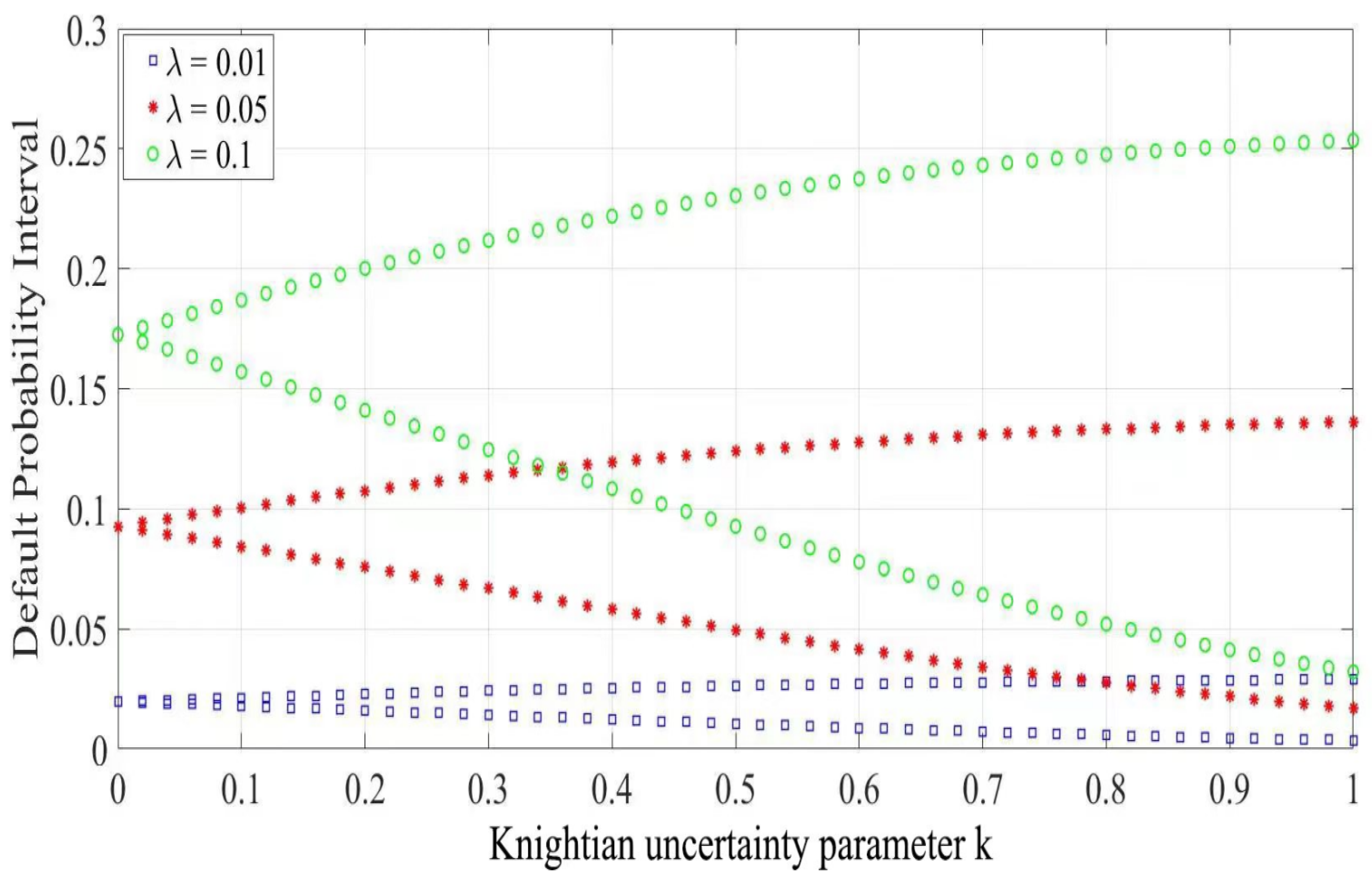
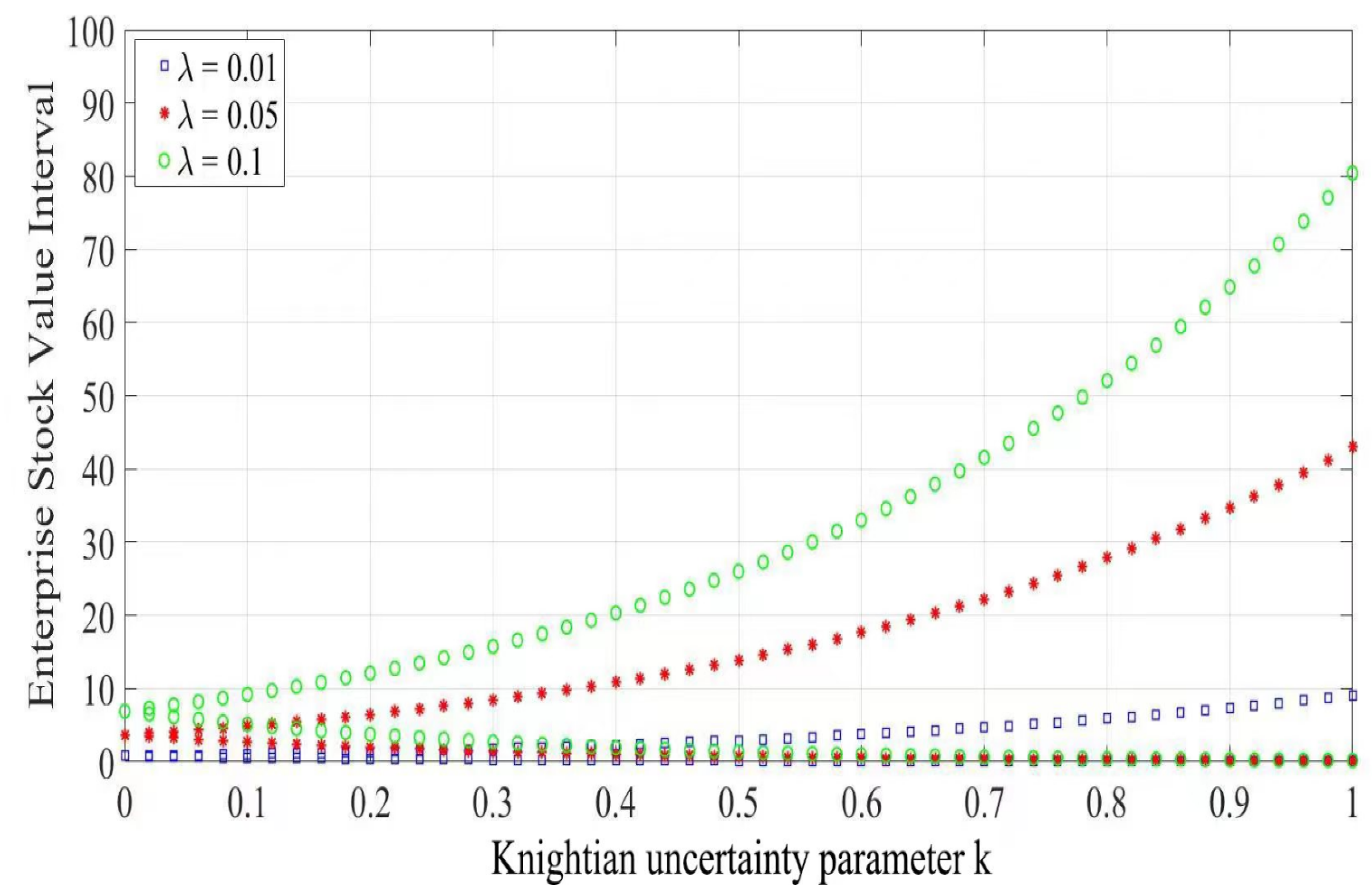
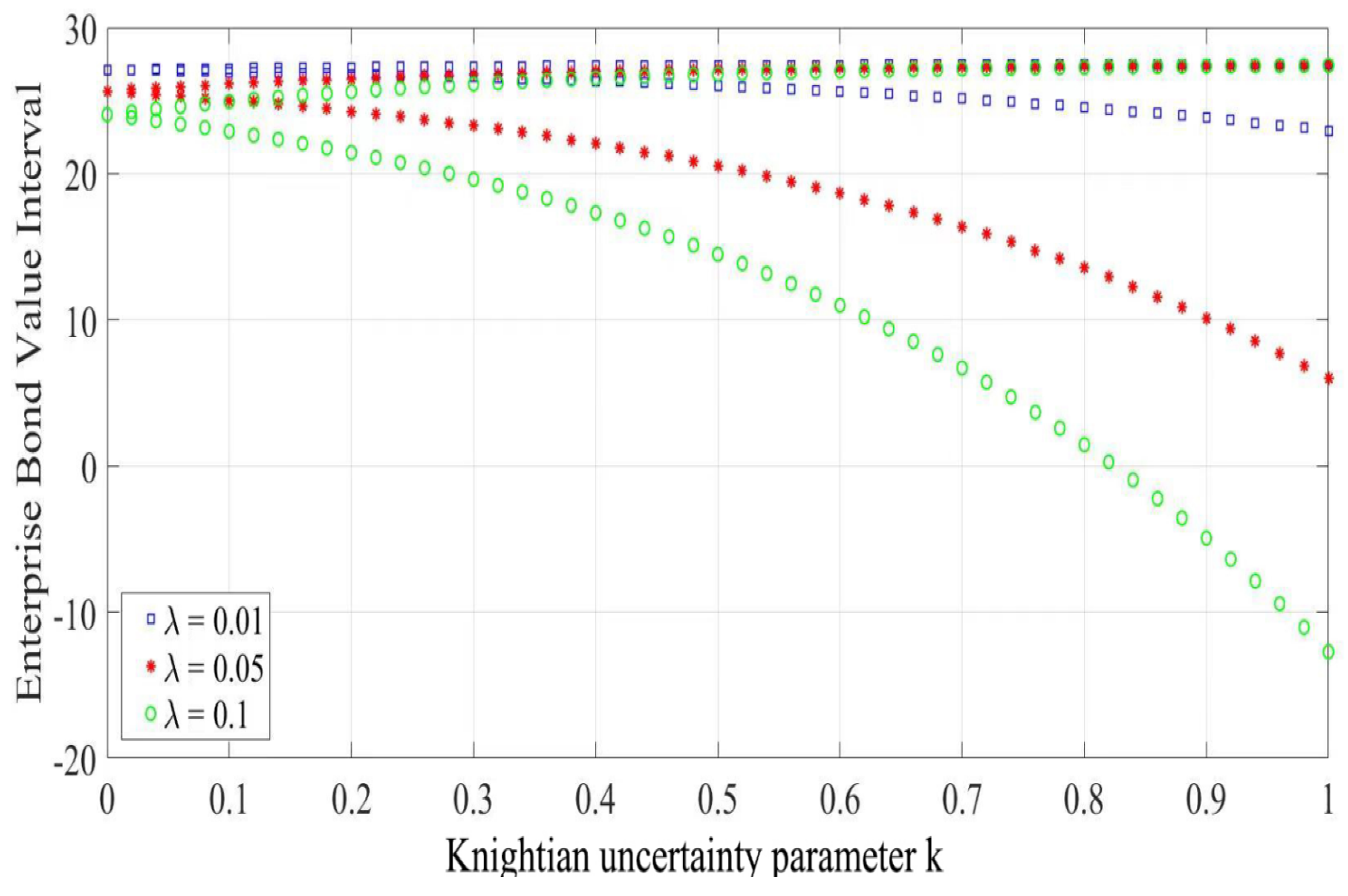
In this part, we examined the effects of the Knightian parameter and Poisson intensity on the three pricing ranges proved above. For calculation convenience, let us assume the value of an enterprise asset at time 0 is $V_0=55$, volatility is ${\sigma }^2=0.04$, the risk free rate of interest is $r=0.05$, the face value of enterprise bonds are $L=50$, enterprise bonds maturity is $T=3$, the mean and volatility of a jump process $(1+U_i)$ are $\overline{\mu }=-0.15$, ${\overline{\sigma }}^2=0.01$, respectively, and the Knightian uncertain parameter is $k\in [0,1]$. From the conclusion of the third section the default probability interval is $[p^{-k},p^k]$, the enterprise stock value interval is $\left[E^k(0,V_0,T),E^{-k}(0,V_0,T)\right]$, and the bond value interval is $\left[D^{-k}(0,V_0,T),D^k(0,V_0,T)\right]$. We take different values of the Poisson intensity $\lambda =0.01,0.05$, and $0.1$, and obtain the following results, Figure 1, Figure 2 and Figure 3.

It can be seen from Figure 1 that the influence on the default probability of the Poisson intensity $\lambda$ and Knightian uncertain parameter was significant. With the increase in Poisson intensity $\lambda$, the probability of default increased significantly. On the other hand, as the Knightian uncertain parameter increased, the company’s default probability became greater and greater, and the default probability interval also gradually increased and the upper bound of the default probability increased, while the lower bound decreased. This meant that the impact of the jump intensity in corporate assets in the financial market on the probability of corporate default could not be ignored.

As shown in Figure 2, the equilibrium price of a call option in a Knightian uncertain environment was no longer a certain value, but an interval. This showed that the information risk and liquidity risk in the financial market, and the resulting changes in investor sentiment (this paper attributed this to Knightian uncertainty), significantly affected the equilibrium price of assets. Due to the objective existence of Knightian uncertainty risks such as information risk and liquidity risk, investors need corresponding uncertainty risk compensation, so the equilibrium price of assets is a certain range.

From Figure 3, we can see that in the Knightian uncertainty environment, the price of a put option is also a range and, whether it is a call option or a put option, as the degree of Knightian uncertainty increased, the pricing range became larger. This showed that the higher the degree of Knightian uncertainty, the greater the uncertainty of future odds or returns. Risk–averse investors not only show Knight uncertainty aversion, and might choose not to enter the market, which reduces the liquidity of the market, but also expect a higher Knight uncertainty premium, showing a larger pricing range.

5. Discussion

From the above analysis, it could be seen that the influence on the default probability, enterprise stock values, and bond value intervals of the Poisson intensity and Knightian uncertain parameter was significant. This showed that if an investor was a knightian uncertainty enthusiast, the more vague they would be about the knightian uncertainty in the financial market and the greater the incentive would be. Conversely, if an investor was knightian uncertainty averse, the more ambiguous they would be about knightian uncertainty in financial markets and the incentive would be less. This result fully demonstrated the impact of Knightian uncertainty on the probability of default, a company’s stock value, and bond value; thus, we must consider the impact of Knightian uncertainty on a company’s default in actual operation. Compared with decisions that do not consider Knight’s uncertain risks, the results of this study took into account investors’ risk appetite and provided a more comprehensive reference for investment decisions. The mainstream asset pricing theory assumed that investors not only clearly know what uncertain states may occur in the future, but also could estimate the probability of their occurrence, and make investment decisions on this basis. However, due to the large amount of uncertainty that actually exists in financial markets, the “premium puzzle” and “smile volatility” have led to a large number of phenomena that deviate from the ideal situation. Researchers call this uncertainty “Knightian uncertainty” and limit the risk to the kind of uncertainty that is unique in probability distributions, quantitatively determinable, closed and complete, while Knightian uncertainty is set as uncertainty that does not have these properties and is subject to frequent changes due to “potential surprises” and novelties. Compared with investment decisions that do not consider Knightian uncertainty risk in Ref. [8], the results of this paper took into account investors’ risk appetite and decision making in different market sentiments, providing a more comprehensive reference for investment decisions.

6. Conclusions

Unlike traditional credit risk models that are based on mainstream asset pricing theory and ignore the impact of uncertainties, such as investor risk appetite and market sentiment, this thesis investigated the credit risk measure of listed companies in a Lévy market under a Knightian uncertainty environment. Assuming that the asset value process of listed companies obeys a Lévy process, a credit risk measure model under a Knightian uncertainty environment was developed. Unlike the traditional credit risk structure model, the probability of default for public companies was no longer a specific number, but an interval. In addition, the effect of Knightian uncertainty on default probability, stock values, and bond values was also investigated using numerical analysis. This differed from previous studies in that the results better reflected the impact of different market sentiments on the default interval and expanded the decision flexibility, which is more conducive to subjective decisions.

This paper stated that an enterprise value is subject to Brownian motion as well as the jump process and Knightian uncertainty is only over Brownian motion. Future research might consider investigating uncertainty over the jump process. This question would be challenging and innovative as jump components are more difficult to estimate than the Brownian motion part. On the other hand, quantifying the strength of Knightian uncertainty in the financial market was a very difficult problem. We currently do not have a better method, so this paper did not involve empirical research for the time being, but only carried out an example analysis. Quantifying Knightian uncertainty risk is also a research direction for us in the future.

References

- Black, F.; Scholes, M. The pricing of options and corporate liabilities. J. Political Econ. 1973, 3, 637–654. [Google Scholar] [CrossRef] [Green Version]
- Merton, R.C. On the pricing of corporate debt: The risk structure of interest rates. J. Financ. 1974, 29, 449–470. [Google Scholar]
- Mason, S.P.; Bhattacharya, S. Risky debt, jump process, and safety covenants. J. Financ. Econ. 1981, 9, 281–307. [Google Scholar] [CrossRef] [Green Version]
- Zhou, C.S. The term structure of credit spreads with jump risk. J. Bank. Financ. 2001, 25, 2015–2040. [Google Scholar] [CrossRef]
- Hilberink, B.; Rogers, L.C. Optimal capital structure and endogenous default. Financ. Stoch. 2002, 6, 237–263. [Google Scholar] [CrossRef]
- Scherer, M. Efficient Pricing Routines of Credit Default Swaps in a Structural Default Model with Jump; University of Ulm: Ulm, Germany, 2005. [Google Scholar]
- Xiong, S. Pricing option on stocks driven by the Lévy jump-diffusion process. J. Shanghai Norm. Univ. (Nat. Sci. Ed.) 2005, 34, 27–31. [Google Scholar]
- Xue, H.; Wang, N. Structural credit risk model driven by Lévy process. J. Shanxi Univ. (Nat. Sci. Ed.) 2008, 31, 406–409. [Google Scholar]
- Shi, Y. Option pricing under a stochastic interest rate mixed index jump diffusion model. Math. Pract. Theory 2021, 51, 87–97. [Google Scholar]
- Knight Frank, H. Risk, Uncertainty and Profit; Houghton Mifflin: Boston, MA, USA, 1921. [Google Scholar]
- Ellsberg, D. Risk, ambiguity and the savage axioms. Q. J. Econ. 1961, 75, 643–669. [Google Scholar] [CrossRef] [Green Version]
- Chen, Z.; Larry, E. Ambiguity, risk, and asset returns in continuous time. Econometrica 2002, 70, 1403–1433. [Google Scholar] [CrossRef]
- Huang, H.; Wang, X.; Liu, Y.; Li, D. Deposit insurance pricing for China’s listed banks under Knight uncertainty. Stat. Inf. Forum 2016, 31, 81–86. [Google Scholar]
- Huang, H.; Wang, X. Option pricing under Knight uncertainty driven by Lévy process. China Sci. Pap. 2017, 12, 554–559. [Google Scholar]
- Liu, F.; Niu, Y.; Zou, Z. Incomplete markets, Knightian uncertainty and high-water marks. Oper. Res. Lett. 2020, 48, 195–201. [Google Scholar] [CrossRef]
- Liu, B. Uncertainty Theory, 2nd ed.; Spring: Berlin, Germany, 2007. [Google Scholar]
- Chen, X. American option pricing formula for uncertain financial market. Eur. J. Oper. Res. 2011, 8, 32–37. [Google Scholar]
- Zhang, Z.; Liu, W. Geometric and average Asian option pricing for uncertain financial market. J. Uncertain Syst. 2014, 8, 317–320. [Google Scholar]
- Sun, J.; Chen, X. Asian option pricing formula for uncertain financial market. J. Uncertain. Anal. Appl. 2015, 3, 11. [Google Scholar] [CrossRef] [Green Version]
- Bentham, E. Option Pricing with Lévy Process; London School of Economics: London, UK, 2000. [Google Scholar]
- David, A. Lévy Process and Stochastic Calculus; Cambridge University Press: Cambridge, UK, 2004. [Google Scholar]
- Zhang, H.; Chen, X.; Nie, X. Robust pricing model of reload stock option under uncertainty. Chin. J. Manag. Sci. 2008, 16, 25–31. [Google Scholar]
- Lin, X. A Study on the Reduced Pricing Model of Credit Derivatives Swaps Based on the Lévy Processes; Southeast University: Dhaka, Bangladesh, 2018. [Google Scholar]
Figure 1.
The variation trend of the default probability interval in Knightian uncertain parameters and the Poisson intensity.
Figure 2.
The variation trend of the enterprise stock value interval in Knightian uncertain parameters and the Poisson intensity.
Figure 3.
The variation trend of the enterprise bond value interval on Knightian uncertain parameters and the Poisson intensity.
Publisher’s Note: MDPI stays neutral with regard to jurisdictional claims in published maps and institutional affiliations. |
© 2022 by the authors. Licensee MDPI, Basel, Switzerland. This article is an open access article distributed under the terms and conditions of the Creative Commons Attribution (CC BY) license (https://creativecommons.org/licenses/by/4.0/).
Share and Cite
MDPI and ACS Style
Huang, H.; Ning, Y.; Chen, X. A Structural Credit Risk Model Driven by the Lévy Process under Knightian Uncertainty. Symmetry 2022, 14, 1041. https://0-doi-org.brum.beds.ac.uk/10.3390/sym14051041
AMA Style
Huang H, Ning Y, Chen X. A Structural Credit Risk Model Driven by the Lévy Process under Knightian Uncertainty. Symmetry. 2022; 14(5):1041. https://0-doi-org.brum.beds.ac.uk/10.3390/sym14051041
Chicago/Turabian StyleHuang, Hong, Yufu Ning, and Xiumei Chen. 2022. "A Structural Credit Risk Model Driven by the Lévy Process under Knightian Uncertainty" Symmetry 14, no. 5: 1041. https://0-doi-org.brum.beds.ac.uk/10.3390/sym14051041
Note that from the first issue of 2016, this journal uses article numbers instead of page numbers. See further details here.