Monitoring the Ratio of Two Normal Variables Based on Triple Exponentially Weighted Moving Average Control Charts with Fixed and Variable Sampling Intervals

Abstract

In statistical process control (SPC), the ratio of two normal random variables (RZ) is a valuable statistical indicator to be taken as the charting statistic. In this work, we propose a triple exponentially weighted moving average (TEWMA) chart for monitoring the RZ. Additionally, the variable sampling interval (VSI) strategy has been adopted to different control charts by researchers. With the application of this strategy, the VSI-TEWMA-RZ chart is then developed to further improve the performance of the proposed TEWMA-RZ chart. The run length (RL) properties of the proposed TEWMA-RZ and VSI-TEWMA-RZ charts are obtained by the widely used Monte-Carlo (MC) simulations. Through the comparisons with the VSI-EWMA-RZ and the VSI-DEWMA-RZ charts, the VSI-TEWMA-RZ chart is statistically more sensitive than the VSI-EWMA-RZ and the VSI-DEWMA-RZ charts in detecting small and moderate shifts. Moreover, it turned out that the VSI-TEWMA-RZ chart has better performance than the TEWMA-RZ chart on the whole. Furthermore, this paper illustrates the implementation of the proposed charts with an example from the food industry.

1. Introduction

The quality of products has become one of the most important factors in the company’s market competition. For improving products’ quality, Statistical Process Control (SPC) offers a lot of tools to supervise and control a process. Control chart, as one of the most critical tools in SPC, is often used to monitor the common or assignable causes. In the SPC literatures, control charts for monitoring the ratio of two normal random variables (RZ) have already been studied extensively. They have been used in various fields—for instance, the baking industry, the pharmaceutical industry, and the industrial production of materials, as seen in [1].

The research on the RZ control charts is mainly divided into three branches: the Shewhart type charts, the cumulative sum (CUSUM) charts and the exponentially weighted moving average (EWMA) charts. Among these three type control charts, the Shewhart control chart for monitoring the RZ was first discussed by Ref. [2], who investigated a quality control procedure for the insurance against unemployment. Ref. [3] pointed out that the distribution of the ratio was extremely complex and the statistical properties of the control chart can only be obtained by simulations. Ref. [4] put forward several guidelines to implement the Shewhart chart for supervising and controlling the ratio of glass oxide composition to its density in the glass industry. Ref. [1] discussed the Shewhart chart based on individual measurements, named as the Shewhart-RZ control chart. Following this work, Ref. [5] studied the RZ chart on the basis that subgroups consist of $n>1$ units. Then, Ref. [6] stated that the synthetic control chart for supervising and controlling the RZ is statistically more sensitive than the Shewhart-RZ chart. As it is known to all, the Shewhart charts are ineffective in detecting small to moderate process shifts. Some researchers have suggested supplementing run rules for improving the Shewhart charts’ statistical properties, see Refs. [7,8,9] and so on. To further improve the Shewhart-RZ chart’s performance, Ref. [10] and Ref. [11] adopted the run rules to the Shewhart-RZ control charts, denoted as RR-RZ control charts for the purpose of increasing its sensitivity to small shifts.

To further overcome the shortcomings of the Shewhart-type charts in detecting a relatively small shift, some researchers have successively proposed EWMA and CUSUM charts. Both types of charts take full advantage use of the previous samples information, making charts faster in detecting relatively small shifts. For example, Refs. [12,13] proposed two one-sided EWMA-RZ charts, and it turned out that the EWMA-RZ chart is statistically more sensitive than the Shewhart -RZ chart on the whole. Additionality, Ref. [14] proposed and studied the statistical properties of two Phase II one-sided CUSUM-RZ control charts and the numerical results showed that the proposed CUSUM chart is more sensitive to small shifts than the Shewhart-RZ chart.

To further improve control charts’ ability to adjust to small shifts, different methods for improving EWMA schemes have been shown in the SPC literature. These charts are considered an extension of EWMA charts. For example, Refs. [15,16] performed the exponential smoothing twice on the weighted coefficients of the EWMA charts, which was named a double exponential weighted moving average (DEWMA) chart. For more works on the DEWMA control charts, the reader may see Refs. [17,18]. Recently, Ref. [19] constructed the one-sided DEWMA chart for time between events (DEWMA-TBE) which has time-varying control limits based on the gamma distribution. It shows that the DEWMA-TBE chart is statistically more sensitive than competitors in detecting downward shifts. Moreover, Ref. [20] have improved the performance of the DEWMA-type control chart with additional run-rule schemes. Since then, Ref. [21] studied the nonparametric DEWMA chart on the basis of the Wilcoxon rank-sum test. Ref. [22] performed the exponential smoothing three times and proposed the triple exponentially weighted moving average (TEWMA) chart for monitoring a normally distributed process. Moreover, a TEWMA chart for monitoring time between events (TBE) was suggested by Ref. [23]. Recently, Ref. [24] proposed a new TEWMA chart for supervising and controlling the process dispersion, moreover the advantage of the chart is shown by comparing with some competitors in detecting small shifts. Later on, a new distribution-free TEWM chart on the basis of the Wilcoxon rank-sum statistic was proposed by Ref. [25]. The studies on the TEWMA chart have demonstrated its outstanding performance in the detection of small shifts.

In the related works of control charts, researchers have found that introducing the variable sampling interval (VSI) strategy to control charts can further improve the performance of traditional charts with a fixed sampling interval (FSI). The VSI strategy is the one that adjusts the next sampling interval based on the position of the current charting statistic on the control chart. For example, Ref. [26] proposed an EWMA-RZ chart by introducing the VSI strategy, denoted as the VSI-EWMA-RZ chart. As a result, the statistical performance of the VSI-EWMA-RZ chart is superior to the traditional EWMA-RZ charts. In addition, Ref. [27] further integrated the VSI into the CUSUM-RZ scheme, called the VSI-CUSUM-RZ chart, to enhance the CUSUM-RZ chart’s performance.

Based on the above studies, it is found that the TEWMA chart has demonstrated its outstanding performance in the detection of small shifts in a normally distributed process. Motivated by this fact, this paper proposes a TEWMA chart for monitoring the RZ. Moreover, since the integration of the VSI strategy can improve the performance of the EWMA-RZ or CUSUM-RZ charts for small to moderate shifts, a VSI-TEWMA-RZ control chart is then proposed to further improve the performance of the proposed TEWMA-RZ chart.

The other parts of this paper are organized as follows: In Section 2, the distribution of the ratio Z between two normal random variables is briefly introduced. Then, the TEWMA-RZ and VSI-TEWMA-RZ charts are introduced in next Section. Section 4 shows the design procedure of the proposed charts. The control limits and the ARL or the average time to signal (ATS) of the proposed charts are also shown in this section by using the widely used Monte-Carlo (MC) simulations. In Section 5, for different chart parameters, the performance of the VSI-TEWMA-RZ chart is compared with the TEWMA-RZ, the VSI-EWMA-RZ, and the VSI-DEWMA-RZ charts. Section 6 takes the food industry as an example and implement the proposed control chart in practice. At last, Section 7 gives several remarkable conclusions and proposals for future research works.

2. A Brief Review of the Distribution of the Ratio Z

In this section, the background of the distribution of the ratio Z is briefly outlined by considering two normally distributed random variables, X and Y—for example $W={(X,Y)}^T\sim N\left({\mathsf{\mu }}_W,{\Sigma }_W\right)$. Here, W is a bivariate normally distributed random vector with a mean vector and variance–covariance matrix, respectively, as below:

$${\mathsf{\mu }}_W=\left(\begin{array}{c}{\mu }_X\\ {\mu }_Y\end{array}\right)$$

(1)

$${\Sigma }_W=\left(\begin{array}{cc}{\sigma }_X^2& \rho {\sigma }_X{\sigma }_Y\\ \rho {\sigma }_X{\sigma }_Y& {\sigma }_Y^2\end{array}\right)$$

(2)

where ρ is the coefficient of correlation between X and Y. According to the definition, the coefficients of variation of the two random variables X and Y are defined as ${\gamma }_X=\frac{{\sigma }_X}{{\mu }_X}$ and ${\gamma }_Y=\frac{{\sigma }_Y}{{\mu }_Y}$, respectively, so the standard-deviation ratio is $\omega =\frac{{\sigma }_X}{{\sigma }_Y}$. Moreover, details of the interested ratio $Z=\frac{X}{Y}$ can refer to Refs. [28,29,30]. Although there is no closed-form expression for the distribution of the ratio Z, it can be approximated by applying a analogical method suggested by Refs. [5,31]. Thus, the approximated expression of the c.d.f. (cumulative distribution function) $F_Z\left(z\mid {\gamma }_X,{\gamma }_Y,\omega ,\rho \right)$ of Z proposed by Ref. [5] can be obtained as follows:

$$F_Z\left(z\mid {\gamma }_X,{\gamma }_Y,\omega ,\rho \right)\simeq \mathsf{\Phi }\left(\frac{A}{B}\right),$$

(3)

where Φ($·$) is the c.d.f. of the standard normal distribution and $A=\frac{z}{{\gamma }_Y}-\frac{\omega }{{\gamma }_X}$ and $B=\sqrt{{\omega }^2-2\rho \omega z+z^2}$ are functions of z, γ_X, γ_Y, ω, and ρ. In addition, the p.d.f. (probability density function) $f_Z\left(z\mid {\gamma }_X,{\gamma }_Y,\omega ,\rho \right)$ of Z can be given as follows:

$$f_Z\left(z\mid {\gamma }_X,{\gamma }_Y,\omega ,\rho \right)\simeq \left(\frac{1}{B{\gamma }_Y}-\frac{\left(z-\rho \omega \right)A}{B^3}\right)\times \varphi \left(\frac{A}{B}\right),$$

(4)

where ϕ ($·$) is the p.d.f. of the standard normal distribution. The i.d.f. (inverse distribution function) $F_Z^{-1}\left(p\mid {\gamma }_X,{\gamma }_Y,\omega ,\rho \right)$ of Z is,

$$F_Z^{-1}\left(p\mid {\gamma }_X,{\gamma }_Y,\omega ,\rho \right)=\{\begin{array}{c}\frac{-C_2-\sqrt{C_2^2-4C_1{C}_3}}{2C_1} \mathrm{if} p\in \left(0,0.5\right],\\ \frac{-C_2+\sqrt{C_2^2-4C_1{C}_3}}{2C_1} \mathrm{if} p\in \left[0.5,1\right).\end{array}$$

(5)

Here, $C_1=\frac{1}{{\gamma }_Y^2}-{\left({\mathsf{\Phi }}^{-1}\left(p\right)\right)}^2$, $C_2=2\omega \left(\rho {\left({\mathsf{\Phi }}^{-1}\left(p\right)\right)}^2-\frac{1}{{\gamma }_X{\gamma }_Y}\right)$ and $C_3={\omega }^2\left(\frac{1}{{\gamma }_X^2}-{\left({\mathsf{\Phi }}^{-1}\left(p\right)\right)}^2\right)$ are functions of γ_X, γ_Y, $p$, ω, and ρ. Moreover, Φ⁻¹($·$) is the i.d.f. of the standard normal distribution.

3. Construction of the TEWMA-RZ Control Charts

To implement the control chart for monitoring the ratio $Z=\frac{X}{Y}$, at each sampling point i = 1,2,…, we collect independent couples $\left\{W_{i,1},W_{i,2},\dots ,W_{i,n}\right\}$ and each $W_{i,j}={\left(X_{i,j},Y_{i,j}\right)}^T\sim N\left({\mathsf{\mu }}_{w,i},{\Sigma }_{w,i}\right)$, j = 1, …, n, is a bivariate normal random vector with a mean vector and variance-covariance matrix, respectively, as follows:

$${\mathsf{\mu }}_{w,i}=\left(\begin{array}{c}{\mu }_{X,i}\\ {\mu }_{Y,i}\end{array}\right),$$

(6)

$${\Sigma }_{w,i}=\left(\begin{array}{cc}{\sigma }_{X,i}^2& {\rho }_0{\sigma }_{X,i}{\sigma }_{Y,i}\\ {\rho }_0{\sigma }_{X,i}{\sigma }_{Y,i}& {\sigma }_{Y,i}^2\end{array}\right).$$

(7)

where ${\rho }_0$ is the defined in-control correlation coefficient between two random variables X and Y. Following Ref. [5], several assumptions are made in this paper. First, the sample units are allowed to change among subgroups, which means ${\mathsf{\mu }}_{w,i}\ne {\mathsf{\mu }}_{w,k}$ and ${\Sigma }_{w,i}\ne {\Sigma }_{w,k}$ for $i\ne k$. Second, for variables X and Y, there is a linear relationship, ${\sigma }_{X,i}={\gamma }_X\times {\mu }_{X,i}$ and ${\sigma }_{Y,i}={\gamma }_Y\times {\mu }_{Y,i}$, where ${\gamma }_X$ and ${\gamma }_Y$ are the supposed known and constant coefficients of the variation of X and Y, respectively. Third, the known in-control value of the ratio is $z_0=\frac{{\mu }_{X,i}}{{\mu }_{Y,i}}$, i = 1, 2, … for the in-control process.

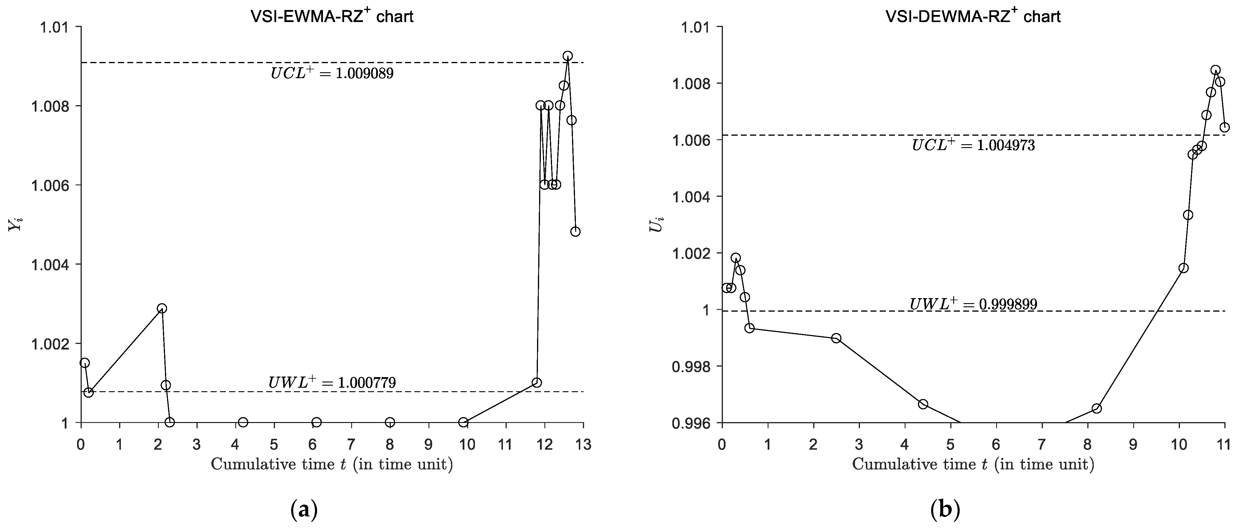
3.1. A Brief Review of the VSI-EWMA-RZ Control Chart

To improve the performance of a Shewhart-RZ chart, Ref. [26] proposed a VSI-EWMA-RZ chart for monitoring the statistic ${\widehat{Z}}_i$,

$${\widehat{Z}}_i=\frac{{\widehat{\mu }}_{X,i}}{{\widehat{\mu }}_{Y,i}}=\frac{{\overline{X}}_i}{{\overline{Y}}_i}=\frac{{\sum }_{j=1}^n{X}_{i,j}}{{\sum }_{j=1}^n{Y}_{i,j}},i=1,2,\dots$$

(8)

As it has been shown in Ref. [5], the c.d.f. $F_{{\widehat{z}}_i}\left(z\mid n,{\gamma }_X,{\gamma }_Y,z_0,\rho \right)$ and the i.d.f $F_{{\widehat{Z}}_i}^{-1}\left(p\mid n,{\gamma }_X,{\gamma }_Y,z_0,{\rho }_0\right)$ of ${\widehat{Z}}_i$ are equal to:

$$F_{{\widehat{z}}_i}\left(z\mid n,{\gamma }_X,{\gamma }_Y,z_0,\rho \right)=F_Z\left(z|\frac{{\gamma }_X}{\sqrt{n}},\frac{{\gamma }_Y}{\sqrt{n}},\frac{z_0{\gamma }_X}{{\gamma }_Y},\rho \right),$$

(9)

$$F_{{\widehat{Z}}_i}^{-1}\left(p\mid n,{\gamma }_X,{\gamma }_Y,z_0,{\rho }_0\right)=F_Z^{-1}\left(p|\frac{{\gamma }_X}{\sqrt{n}},\frac{{\gamma }_Y}{\sqrt{n}},\frac{z_0{\gamma }_X}{{\gamma }_Y},{\rho }_0\right),$$

(10)

where $F_Z\left(z\mid \frac{{\gamma }_X}{\sqrt{n}},\frac{{\gamma }_Y}{\sqrt{n}},\frac{z_0{\gamma }_X}{{\gamma }_Y},\rho \right)$ is the c.d.f. of Z in Equation (3) and $F_Z^{-1}\left(p\mid \frac{{\gamma }_X}{\sqrt{n}},\frac{{\gamma }_Y}{\sqrt{n}},\frac{z_0{\gamma }_X}{{\gamma }_Y},{\rho }_0\right)$ is the i.d.f. of Z in Equation (5).

For detecting the upward shifts, the statistic $Y_i^{+}$ of the upper-sided VSI-EWMA-RZ (denoted as VSI-EWMA-RZ⁺) chart is defined as:

$$Y_i^{+}=\max \left(z_0,\left(1-{\lambda }^{+}\right)Y_{i-1}^{+}+{\lambda }^{+}{\widehat{Z}}_i\right), Y_0^{+}=z_0,$$

(11)

With an upper control limit $UC{L}^{+}=K^{+}\times z_0$, where ${\lambda }^{+}\in \left(0,1\right]$ is the smoothing parameter and $K^{+}>1$ is chart parameter of the VSI-EWMA-RZ⁺ chart. In addition, an upper warning limit $UW{L}^{+}=W^{+}\times z_0$ between [$z_0,UC{L}^{+}$] is added to the chart, where $W^{+}<K^{+}$ is the upper warning limit coefficient. A process is deemed to be out-of-control if the statistic $Y_i^{+}>UC{L}^{+}.$ Otherwise, the process is thought to be in-control if the statistic $Y_i^{+}$ falls within the warning region $\left(UW{L}^{+}, UC{L}^{+}\right]$, and a shorter sampling interval $h_s$ is used to collect the next sampling point. The process is deemed to be in-control if the plotted statistic $Y_i^{+}$ falls within the safe region $[z_0,UW{L}^{+}]$, and a longer sampling interval $h_L$ is used.

Similarly, for the detection of downward shifts, the statistic $Y_i^{-}$ of the lower-sided VSI-EWMA-RZ (denoted as VSI-EWMA-RZ⁻) chart is defined as:

$$Y_i^{-}=\min \left(z_0,\left(1-{\lambda }^{-}\right)Y_{i-1}^{-}+{\lambda }^{-}{\widehat{Z}}_i\right), Y_0^{-}=z_0,$$

(12)

With a lower control limit $LC{L}^{-}=K^{-}\times z_0$, where ${\lambda }^{-}\in \left(0,1\right]$ is the smoothing parameter and $K^{-}<1$ is the chart parameter of the VSI-EWMA-RZ⁻ chart, respectively. In addition, a lower warning limit $LW{L}^{-}=W^{-}\times z_0$ between [$LC{L}^{-},z_0$] is added to the chart, where $W^{-}>K^{-}$ is the lower warning limit coefficient. A process is claimed to be out-of-control if the plotted statistic $Y_i^{-}<LC{L}^{-}.$ Otherwise, the process is deemed to be in-control if the plotted statistic $Y_i^{-}$ falls within the warning region $\left[LC{L}^{-}LW{L}^{-}\right)$ and a shorter sampling interval $h_s$ is used. The process is deemed to be in-control if the plotted statistic $Y_i^{-}$ falls within the safe region $[LW{L}^{-},z_0]$ and a longer sampling interval $h_L$ is used.

3.2. A Brief Review of the VSI-DEWMA-RZ Chart

According to Ref. [32], the one-sided VSI-DEWMA-RZ charts are constructed by making the smoothing twice and are defined as follows:

An upward VSI-DEWMA-RZ (denoted as VSI-DEWMA-RZ⁺) chart is used to detect an increase in the process and the monitoring statistic $U_i^{-}$ is:

$$Y_i^{+}={\lambda }^{+}{\widehat{Z}}_i+\left(1-{\lambda }^{+}\right)Y_{i-1}^{+},Y_0^{+}=z_0,$$

(13)

$$U_i^{+}={\lambda }^{+}{Y}_i^{+}+\left(1-{\lambda }^{+}\right)U_{i-1}^{+},U_0^{+}=z_0,$$

(14)

where ${\lambda }^{+}\in \left(0,1\right]$ is the smoothing parameter and $K^{+}>1$ is the chart parameter of the VSI-DEWMA-RZ⁺ chart, respectively. The single control limit of the chart is $UC{L}^{+}=K^{+}\times z_0$. Also, an upper warning limit $UW{L}^{+}=W^{+}\times z_0$ between $\left[z_0,UC{L}^{+}\right]$ is added, where $W^{+}<K^{+}$ is the upper warning limit coefficient. If the plotted statistic $U_i^{+}>UC{L}^{+},$ the process is considered to be out-of-control. Otherwise, the process is claimed to be in-control if $UW{L}^{+}<U_i^{+}\le UC{L}^{+}$ and a shorter sampling interval $h_s$ is used to collect the next sampling point. The process is considered to be in-control if $z_0\le U_i^{+}\le UW{L}^{+}$ and a longer sampling interval $h_L$. is used. The sampling interval $h_i$ can be expressed as follows:

$$h_i=\{\begin{array}{l}{h}_s,UW{L}^{+}<U_i^{+}\le UC{L}^{+}\\ h_L, U_i^{+}\le UW{L}^{+}\end{array}$$

(15)

A downward VSI-DEWMA-RZ (denoted as VSI-DEWMA-RZ⁻) chart is used to detect a decrease in the process and the statistic $U_i^{-}$ can be similarly defined as:

$$Y_i^{-}={\lambda }^{-}{\widehat{Z}}_i+\left(1-{\lambda }^{-}\right)Y_{i-1}^{-},Y_0^{-}=z_0,$$

(16)

$$U_i^{-}={\lambda }^{-}{Y}_i^{-}+\left(1-{\lambda }^{-}\right)U_{i-1}^{-},U_0^{-}=z_0,$$

(17)

where ${\lambda }^{-}\in \left(0,1\right]$ and $K^{-}<1$ are the smoothing and chart parameters of the FSI-DEWMA-RZ-chart, respectively. The single control limit of the chart is $LC{L}^{-}=K^{-}\times z_0$. A lower warning limit $LW{L}^{-}=W^{-}\times z_0$ between $\left[LC{L}^{-},z_0\right]$ is added, where $W^{-}>K^{-}$ is the lower warning limit coefficient. If the plotted statistic $U_i^{-}<LC{L}^{-}$, the process is considered to be out-of-control. Otherwise, the process is claimed to be in-control if $LC{L}^{-}\le U_i^{-}<LW{L}^{-}$ and a shorter sampling interval $h_s$ is used. The process is considered to be in-control if $LW{L}^{-}\le U_i^{-}\le z_0$ and a longer sampling interval $h_L$ is used. The sampling interval $h_i$ can be expressed in a form similar to Equation (15).

3.3. The Proposed TEWMA-RZ Charts

To further enhance the advantage of the FSI- or VSI-EWMA-RZ charts, this paper performs the exponential smoothing three times on the weighted coefficients of the EWMA charts. As the distribution of Z is non-symmetric, two separate one-sided TEWMA-RZ charts are proposed for detecting increasing and decreasing shifts, respectively. Moreover, the VSI-TEWMA-RZ chart is further proposed to increase the sensitivity of the FSI-TEWMA-RZ chart.

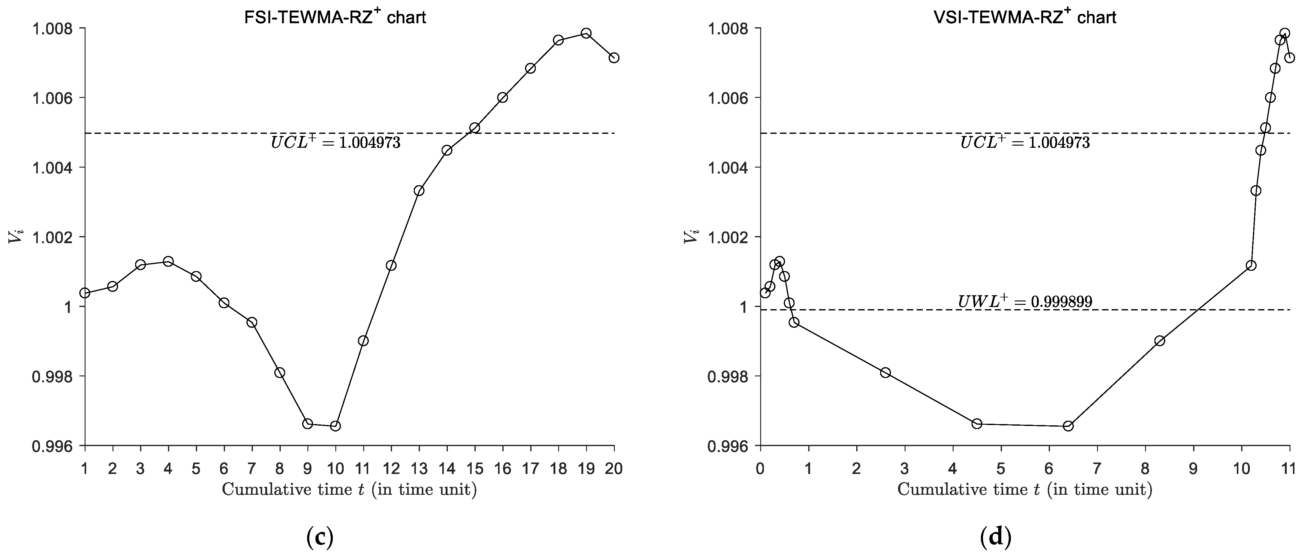
3.3.1. The FSI-TEWMA-RZ Chart

An upward FSI-TEWMA-RZ (denoted as FSI-TEWMA-RZ⁺) chart is used to detect an increase in the process, and the monitoring statistic $V_i^{+}$ is:

$$Y_i^{+}={\lambda }^{+}{\widehat{Z}}_i+\left(1-{\lambda }^{+}\right)Y_{i-1}^{+},Y_0^{+}=z_0,$$

(18)

$$U_i^{+}={\lambda }^{+}{Y}_i^{+}+\left(1-{\lambda }^{+}\right)U_{i-1}^{+},U_0^{+}=z_0,$$

(19)

$$V_i^{+}={\lambda }^{+}{U}_i^{+}+\left(1-{\lambda }^{+}\right)V_{i-1}^{+},V_0^{+}=z_0,$$

(20)

where ${\lambda }^{+}\in \left(0,1\right]$ is the smoothing parameter and $K^{+}>1$ is the chart parameter of the FSI-TEWMA-RZ⁺ chart, respectively. The single control limit of the chart is $UC{L}^{+}=K^{+}\times z_0$. A process is deemed to be out-of-control if the statistic $V_i^{+}$ falls above the $UC{L}^{+}$. Otherwise, the process is declared to be in-control.

A downward FSI-TEWMA-RZ (denoted as FSI-TEWMA-RZ⁻) chart is used to detect downward process sifts and the statistic $V_i^{-}$ can be similarly defined as:

$$Y_i^{-}={\lambda }^{-}{\widehat{Z}}_i+\left(1-{\lambda }^{-}\right)Y_{i-1}^{-},Y_0^{-}=z_0,$$

(21)

$$U_i^{-}={\lambda }^{-}{Y}_i^{-}+\left(1-{\lambda }^{-}\right)U_{i-1}^{-},U_0^{-}=z_0,$$

(22)

$$V_i^{-}={\lambda }^{-}{U}_i^{-}+\left(1-{\lambda }^{-}\right)V_{i-1}^{-},V_0^{-}=z_0,$$

(23)

where ${\lambda }^{-}\in \left(0,1\right]$ is the smoothing parameter and $K^{-}<1$ is the chart parameter of the TEWMA-RZ⁻ chart, respectively. The single control limit of the chart is $LC{L}^{-}=K^{-}\times z_0$. A process is deemed to be out-of-control if the charting statistic $V_i^{-}$ falls below the $LC{L}^{-}$. Otherwise, the process is declared to be in-control.

3.3.2. The VSI-TEWMA-RZ Chart

For further enhancing the sensitivity of the FSI-TEWMA-RZ chart for small or moderate shifts in the process, this paper introduces the VSI strategy into the FSI-TEWMA-RZ control chart in Section 3.3.1.

With respect to the proposed VSI-TEWMA-RZ chart, the control limit $UC{L}^{+}\left(LC{L}^{-}\right)$ is consistent with the FSI-TEWMA-RZ chart. For the upward VSI-TEWMA-RZ (denoted as VSI-TEWMA-RZ⁺) control chart, an upper warning limit $UW{L}^{+}=W^{+}\times z_0$ between [$z_0,UC{L}^{+}$] is added, where $W^{+}<K^{+}$ is the upper warning limit coefficient. If the plotted statistic $V_i^{+}>UC{L}^{+},$ the process is considered to be out-of-control. Otherwise, the process is claimed to be in-control if $UW{L}^{+}<V_i^{+}\le UC{L}^{+}$ and a shorter sampling interval $h_s$ is used to collect the next sampling point. The process is considered to be in-control if $z_0\le V_i^{+}\le UW{L}^{+}$ and a longer sampling interval $h_L$ is used. The sampling interval $h_i$ can be expressed as follows:

$$h_i=\{\begin{array}{c}{h}_s,UW{L}^{+}<V_i^{+}\le UC{L}^{+}\\ h_L, V_i^{+}\le UW{L}^{+}\end{array}$$

(24)

In terms of the downward VSI-TEWMA-RZ (denoted as VSI-TEWMA-RZ⁻) control chart, a lower warning limit $LW{L}^{-}=W^{-}\times z_0$ between [$LC{L}^{-},z_0$] is added, where $W^{-}>K^{-}$ is the lower warning limit coefficient. If the plotted statistic $V_i^{-}<LC{L}^{-}$, the process is considered to be out-of-control. Otherwise, the process is claimed to be in-control if $LC{L}^{-}\le V_i^{-}<LW{L}^{-}$ and a shorter sampling interval $h_s$ is used. The process is considered to be in-control if $LW{L}^{-}\le V_i^{-}\le z_0$ and a longer sampling interval $h_L$ is used. The sampling interval $h_i$ can be expressed in a form similar to Equation (24).

4. Design of the Proposed TEWMA-RZ Charts

4.1. Design of the Proposed FSI-TEWMA-RZ Chart

Because of the complexity of the charting statistic of the FSI-TEWMA-RZ chart, the run length (RL) properties of the control chart are obtained by the MC simulation in this paper. Furthermore, to evaluate the performance of the FSI-TEWMA-RZ chart, the ARL measure, which indicates the average number of samples collected before going into out-of-control state, is selected. When the process is under control, the ARL is recorded as $AR{L}_0$. Otherwise, when the process gets out of control, the ARL is recorded as $AR{L}_1$. For illustration, the detailed procedure of the MC simulation of the FSI-TEWMA-RZ⁺ chart is summarized as follows:

Step 1 Select the values of the sample size n, the in-control ratio $z_0$, the smoothing parameter ${\lambda }^{+}$, and the chart coefficient $K^{+}$. Compute the corresponding control limit $UC{L}^{+}=K^{+}\times z_0$.

Step 2 Generate a random sample from a multivariate normal distribution and compute the value of the charting statistic $V_i^{+}$ as in Equation (20).

Step 3 If the charting statistic $V_i^{+}$ falls below the $UC{L}^{+}$, the process is deemed to be in-control and returns to Step 2. Otherwise, the process is deemed to be out-of-control and then record the RL values.

Step 4 Repeat Steps 2 and 3 for . times, calculate the ARL values from the recorded RL values. The approximated expressions of the ARL can be written as:

$$ARL=\frac{{\sum }_{t=1}^{N}R{L}_t}{N},t=1,\dots ,N$$

(25)

Without loss of generality, this paper assumes ARL₀ = 200 and further studies the $AR{L}_1$ performance of the proposed chart under different shifts. The performance of the FSI-TEWMA-RZ chart can be expressed as:

$$AR{L}_1=AR{L}_1\left(n,\lambda ,K,{\gamma }_X,{\gamma }_Y,z_0,\rho ,\tau \right),$$

(26)

Subject to the constraint:

$$ARL\left(n,\lambda ,K,{\gamma }_X,{\gamma }_Y,z_0,\rho ,\tau =1\right)=AR{L}_0.$$

(27)

When $\tau =1$, the process is under control. Otherwise, when $\tau \ne 1$, the process is returns to be out-of-control. For the above model, considering different parameter combinations, this paper uses a bisection search algorithm to computer the value of K that satisfies the constraint of $AR{L}_0=200$, and then it is used to compute the $AR{L}_1$ values of the proposed chart.

4.2. Design of the Proposed VSI-TEWMA Charts

Since the sampling interval between the consecutive samples varies, it is not reasonable to assess the performance of the VSI-TEWMA-RZ chart by the ARL measure. Thus, the ATS is used to evaluate the performance of the VSI-TEWMA-RZ chart. The ATS represents the anticipant time before a control chart triggers an out-of-control signal. When the process is under control, it is recorded as $AT{S}_0$. Otherwise, when the process gets out-of-control, it is recorded as $AT{S}_1$.

For the FSI-TEWMA-RZ chart, the sampling interval h is fixed, which indicates that the $AT{S}^{FSI}=h\times AR{L}^{FSI}$. In general, the sampling interval of the FSI control chart is usually equal to one, that is, $h=1$. Since the sampling interval $h_i$ depends on the position of the currently monitoring statistic on the control chart, then the $AT{S}^{VSI}=E\left(h_i\right)\times AR{L}^{VSI}$, where $E\left(h_i\right)$ stands for the average sampling interval (ASI) of the VSI type chart. The detailed procedure of the MC simulation of the VSI-TEWMA-RZ⁺ chart is summarized as below:

Step 1 Select the values of the sample size n, the in-control ratio $z_0$, the smoothing parameter ${\lambda }^{+}$, and the warning limit coefficient $W^{+}$ and $K^{+}$. Compute the corresponding warning limit $UW{L}^{+}=W^{+}\times z_0$ and the control limit $UC{L}^{+}=K^{+}\times z_0$.

Step 2 Generate a random sample from a multivariate normal distribution and compute the value of the charting statistic $V_i^{+}$ as in Equation (20).

Step 3 If $UW{L}^{+}<V_i^{+}\le UC{L}^{+}$, a shorter sampling interval $h_s$ is used to collect the next sampling point, and if $V_i^{+}\le UW{L}^{+}$, a longer sampling interval $h_L$ is used to collect the next sampling point. Then, the process is declared to be in-control and returns to Step 2. The times $t_S$ and $t_L$ of the sampling intervals $h_s$ and $h_L$ are recorded, respectively. Otherwise, if the $V_i^{+}$ falls above the $UC{L}^{+}$, the process is declared to be out-of-control.

Step 4 Repeat Steps 2 and 3 for $N={10}^5$ times, calculate the ATS values from the recorded times of the sampling intervals $h_s$ and $h_L$. The approximated expressions of the ATS can be written as:

$$ATS=h_S+h_S\times \frac{{\sum }_{t=1}^N{t}_S}{N}+h_L\times \frac{{\sum }_{t=1}^N{t}_L}{N},t=1,\dots ,N$$

(28)

Similarly, this paper assumes $AT{S}_0=200$ and further studies the $AT{S}_1$ performance of the proposed control charts under different process shifts.

The expressions of $AT{S}^{FSI}$ and $AT{S}^{VSI}$ are given as follows:

$$\{\begin{array}{c}AT{S}^{VSI}=AT{S}^{VSI}\left(n,h_S,h_L,\lambda ,K,W,{\gamma }_0,{\gamma }_1,z_0,\rho ,\tau \right)\\ AT{S}^{FSI}=h\times AR{L}_1^{FSI}\left(n,\lambda ,K,{\gamma }_0,{\gamma }_1,z_0,\rho ,\tau \right)\end{array},$$

(29)

For the purpose of comparing the performance of the FSI-TEWMA-RZ and the VSI-TEWMA-RZ control charts, it is necessary to make sure that the control charts have the same controlled performance. The out-of-control performance of the VSI-TEWMA-RZ chart can be expressed as below:

$$AT{S}_1^{VSI}=AT{S}_1^{VSI}\left(n,h_S,h_L,\lambda ,K,W,{\gamma }_0,{\gamma }_1,z_0,\rho ,\tau \right)$$

Subject to the constraint:

$$AT{S}_0^{VSI}=AT{S}_0^{FSI}$$

(30)

$$AS{I}_0=h=1,$$

(31)

where $AS{I}_0$. is the controlled ASI of the VSI-TEWMA-RZ chart. Following the research work of Ref. [33], a general formula to determine the value of $h_S$ and $h_L$ are as follows:

$${\rho }_S{h}_S+{\rho }_L{h}_L=h=1 \mathrm{and} {\rho }_S+{\rho }_L=1$$

(32)

where ${\rho }_S$ and ${\rho }_L$ are the probabilities that the statistic $V_i$ falls into the warning area and the safe area when the process is controlled, respectively. According to the research work of Ref. [34], this paper selects $\left(h_S,h_L\right)=\left(0.1,1.9\right)$ and ${\rho }_S={\rho }_L=0.5$ for illustration.

In addition, a bisection search algorithm is used to calculate the control limit coefficient K and warning limit coefficient W by satisfying the constraint of $AT{S}_0=200$ and $AS{I}_0=1$. Then, these parameters are used to calculate the out-of-control $AT{S}_1$ values for the different process shift τ. According to the research of Ref. [26], we assume $z_0=1$ and select $\lambda \in \left\{0.2,0.5\right\}$ and $n\in \left\{1,5\right\}$ to discuss the performance of the VSI-TEWMA-RZ chart. For the selected combinations of $\left(n, \lambda \right)$,

Table 1. K⁺ and W⁺ values of the VSI-TEWMA-RZ chart when $AT{S}_0=200$.

$\lambda$	$\mathbf{\left(}{\mathit{\gamma }}_{\mathit{x}} \mathbf{=} \mathit{0.01}\mathbf{,}{\mathit{\gamma }}_{\mathit{Y}} \mathbf{=} \mathbf{0.01}\mathbf{\right)}$				$\mathbf{\left(}{\mathit{\gamma }}_{\mathit{x}} \mathbf{=} \mathbf{0.2}\mathbf{,}{\mathit{\gamma }}_{\mathit{Y}} \mathbf{=} \mathbf{0.2}\mathbf{\right)}$
	$\mathit{n} \mathbf{=} \mathbf{1}$		$\mathit{n} \mathbf{=} \mathbf{5}$		$\mathit{n} \mathbf{=} \mathbf{1}$		$\mathit{n} \mathbf{=} \mathbf{5}$
	$\mathit{K}$	$\mathit{W}$	$\mathit{K}$	$\mathit{W}$	$\mathit{K}$	$\mathit{W}$	$\mathit{K}$	$\mathit{W}$
	${\rho }_0={\rho }_1=-0.8$
0.2	1.0067	0.9998	1.0030	0.9999	1.2480	1.0601	1.0762	1.0083
0.5	1.0161	1.0000	1.0071	0.9999	1.5315	1.0581	1.1699	1.0106
	${\rho }_0={\rho }_1=-0.4$
0.2	1.0059	0.9998	1.0026	0.9999	1.2061	1.0467	1.0653	1.0061
0.5	1.0141	0.9999	1.0063	1.0000	1.4454	1.0452	1.1466	1.0069
	${\rho }_0={\rho }_1=0$
0.2	1.0050	0.9998	1.0022	0.9999	1.1618	1.0316	1.0534	1.0042
0.5	1.0119	0.9999	1.0053	1.0000	1.3544	1.0305	1.1210	1.0047
	${\rho }_0={\rho }_1=0.4$
0.2	1.0038	0.9998	1.0017	0.9999	1.1146	1.0179	1.0397	1.0019
0.5	1.0092	0.9999	1.0041	1.0000	1.2543	1.0179	1.0912	1.0028
	${\rho }_0={\rho }_1=0.8$
0.2	1.0022	0.9999	1.0010	1.0000	1.0574	1.0045	1.0216	1.0002
0.5	1.0053	1.0000	1.0024	1.0000	1.1316	1.0051	1.0504	1.0008

shows the values of K⁺ and W⁺ of the VSI-TEWMA-RZ control chart. Considering the space limitation, this article only gives the values of K⁺ and W⁺ under the condition that ${\gamma }_X={\gamma }_Y$. It is noted that the value of K⁺ of the VSI-TEWMA-RZ chart presented in Table 1, which is the same as the one from the corresponding FSI-TEWMA-RZ chart.

5. Numerical Results and Analysis

This section first compares the performance of the proposed VSI-TEWMA-RZ chart and the corresponding FSI-TEWMA-RZ control chart, and then compares the VSI-TEWMA-RZ chart’s performance with the VSI-DEWMA-RZ chart in Ref. [32] and the VSI-EWMA-RZ chart proposed by Ref. [26]. Similar to the scenarios of Ref. [26], the parameter settings of the simulations are $\lambda \in \left\{0.2,0.5\right\}$, $n\in \left\{1,5\right\}$, ${\gamma }_X\in \left\{0.01,0.2\right\}$, ${\gamma }_Y\in \left\{0.01,0.2\right\}$ and ${\rho }_0\in \left\{-0.8,-0.4,0,0.4,0.8\right\}$, under different conditions $\left\{({\gamma }_X={\gamma }_Y,{\rho }_0={\rho }_1), \left({\gamma }_X\ne {\gamma }_Y,{\rho }_0={\rho }_1\right), \left({\rho }_0\ne {\rho }_1,{\gamma }_X={\gamma }_Y\right),\left({\rho }_0\ne {\rho }_1,{\gamma }_X\ne {\gamma }_Y\right)\right\}$. Since the proposed VSI-TEWMA-RZ control chart is mainly used to advance the sensitivity of the RZ chart for monitoring small shifts in a process and let us take the upward control chart for instance, we give priority to the performance of the RZ charts for the upward shifts $\mathsf{\tau }\in \left\{1.001, 1.005, 1.01, 1.02, 1.05\right\}$.

5.1. Comparisons between the VSI-TEWMA-RZ and the FSI-TEWMA-RZ Charts

According to the above parameter settings and the values of K⁺ and W⁺ presented in Table 1, Figure 1, Figure 2, Figure 3 and Figure 4 compare the performance of the upper-sided FSI-TEWMA-RZ and VSI-TEWMA-RZ charts when monitoring the upward shifts. The $AR{L}_1$ and $AT{S}_1$ represent the performances of the corresponding FSI and VSI control charts, respectively. It is pointed out that since the sampling interval of the FSI chart is $h=1$, the FSI chart’s ARL is equal to its ATS value. Then, the $AR{L}_1$ performance of the FSI chart can be directly compared with the $AT{S}_1$ performance of the VSI chart.

Figure 1 and Figure 2 show the out-of-control $AR{L}_1$ values of the FSI-TEWMA-RZ and the $AT{S}_1$ values of the proposed VSI-TEWMA-RZ chart under the conditions that $\left({\gamma }_X={\gamma }_Y, {\rho }_0={\rho }_1\right)$ and (${\gamma }_X\ne {\gamma }_Y, {\rho }_0={\rho }_1)$, respectively. In Figure 1 and Figure 2, when the process is in an out-of-control state, there is no shift in the correlation between X and Y, that is $\rho ={\rho }_0={\rho }_1$. From the results presented in Figure 1 and Figure 2, some conclusions can be drawn as follows:

Generally, the proposed VSI-TEWMA-RZ chart reacts faster than the proposed FSI-TEWMA-RZ chart for detecting the process shifts. For instance, when $\left({\gamma }_X,{\gamma }_Y\right)=\left(0.01,0.01\right), n=1, \lambda =0.2, \tau =1.001$, and ${\rho }_0={\rho }_1=-0.8$, we obtain $AT{S}_1=111.5$ for the VSI-TEWMA-RZ chart, which is much smaller than the $AR{L}_1=130.7$ for the FSI-TEWMA-RZ chart in Figure 1.

The performances of the proposed FSI- and VSI-TEWMA-RZ charts are greatly affected by $\left({\gamma }_X,{\gamma }_Y\right)$. When ${\gamma }_X={\gamma }_Y$, the smaller the coefficients of variation $\left({\gamma }_X,{\gamma }_Y\right)$, the better the performances of the proposed FSI- and VSI-TEWMA-RZ charts. For example, when ${\rho }_0={\rho }_1=0.4$, $n=1$, $\lambda =0.2$, and $\tau =1.01$ in Figure 1, we have $AT{S}_1=10.2$ for the FSI-TEWMA-RZ chart and $AT{S}_1=1.3$ for the VSI-TEWMA-RZ chart when $\left({\gamma }_X,{\gamma }_Y\right)=\left(0.01,0.01\right)$. As a contrast, we have $AT{S}_1=146.0$ for the FSI-TEWMA-RZ chart and $AT{S}_1=130.6$ for the VSI-TEWMA-RZ chart when $\left({\gamma }_X,{\gamma }_Y\right)$ increases up to $\left(0.2,0.2\right)$.

The performances of the proposed FSI- and VSI-TEWMA-RZ charts depend on ${\rho }_0$ and ${\rho }_1$. The performances of the proposed FSI- and VSI-TEWMA-RZ charts improve when ${\rho }_0$ increases. For example, when $\left({\gamma }_X,{\gamma }_Y\right)=\left(0.01,0.01\right)$, $n=1$, $\lambda =0.5$,$\tau =1.001$, and ${\rho }_0={\rho }_1=-0.8$, we have $AT{S}_1=144.9$ for the FSI-TEWMA-RZ chart and $AT{S}_1=132.3$ for the VSI-TEWMA-RZ chart in Figure 1. As a contrast, we obtain $AT{S}_1=82.1$ for the FSI-TEWMA-RZ chart and $AT{S}_1=60.2$ when ${\rho }_0$ and ${\rho }_1$ increase up to (0.8,0.8)$.$ The performances of the proposed FSI- and VSI-TEWMA-RZ charts are influenced by λ. The FSI- and VSI-TEWMA-RZ charts have a better performance in detecting small shifts when $\lambda$ is generally small. As λ increases, their ability to detect small shifts gradually deteriorates. Instead, these charts are more sensitive to large shifts. For instance, when $\left({\gamma }_X,{\gamma }_Y\right)=\left(0.2,0.2\right)$, ${\rho }_0={\rho }_1=0.8$, $n=5$, and $\tau =1.001$, we obtain $AT{S}_1=174.6$ for the FSI-TEWMA-RZ chart and $AT{S}_1=164.4$ for the VSI-TEWMA-RZ chart when $\lambda =0.2$ in Figure 1. If $\lambda$ increases up to 0.5, we obtain $AT{S}_1=179.8$ for the FSI-TEWMA-RZ chart and $AT{S}_1=175.9$ for the VSI-TEWMA-RZ chart, which are larger than the ones of the $\lambda =0.2$ case, respectively. Moreover, for a larger shift $\tau =1.05$, we obtain $AT{S}_1=11$ for the FSI-TEWMA-RZ chart and $AT{S}_1=2.5$ for the VSI-TEWMA-RZ chart when $\lambda =0.2$ in Figure 1. If $\lambda$ increases up to 0.5, we obtain $AT{S}_1=9.1$ for the FSI-TEWMA-RZ chart and $AT{S}_1=2.0$ for the VSI-TEWMA-RZ chart, which are smaller than the ones of the $\lambda =0.2$ case, respectively.

Figure 3 and Figure 4 show the $AR{L}_1$ values of the FSI-TEWMA-RZ chart and the $AT{S}_1$ values of the proposed VSI-TEWMA-RZ chart under the conditions that $({\gamma }_X={\gamma }_Y, {\rho }_0\ne {\rho }_1$) and (${\gamma }_X\ne {\gamma }_Y, {\rho }_0\ne {\rho }_1)$, respectively. It is worth noting that the correlation coefficient between X and Y changes, that is ${\rho }_0\ne {\rho }_1$. In order to facilitate the comparison and to be consistent with the research of Ref. [26], this paper chooses the in-control correlation coefficient ${\rho }_0=\pm 0.4$ and the values of the studied shift in the correlation are 0.5 and 2, that is ${\rho }_1=0.5\times {\rho }_0$ and ${\rho }_1=2\times {\rho }_0$. From Figure 3 and Figure 4, some conclusions can be summarized as follows:

Figure 3. ARL values of the FSI-TEWMA-RZ (-○-) chart, ATS values of the VSI-DEWMA-RZ (-☆-), VSI-TEWMA-RZ (-□-), and VSI-EWMA-RZ (-✳-) charts for ${\gamma }_X\in \left\{0.01,0.2\right\}, {\gamma }_Y\in \left\{0.01,0.2\right\}, {\gamma }_X={\gamma }_Y, {\rho }_0\in \left\{-0.8,-0.4,0,0.4,0.8\right\}, {\rho }_0\ne {\rho }_1, \tau \in \left\{1.001,1.005,1.01,1.02,1.05\right\} \mathrm{and} n\in \left\{1,5\right\}$.

Figure 3. ARL values of the FSI-TEWMA-RZ (-○-) chart, ATS values of the VSI-DEWMA-RZ (-☆-), VSI-TEWMA-RZ (-□-), and VSI-EWMA-RZ (-✳-) charts for ${\gamma }_X\in \left\{0.01,0.2\right\}, {\gamma }_Y\in \left\{0.01,0.2\right\}, {\gamma }_X={\gamma }_Y, {\rho }_0\in \left\{-0.8,-0.4,0,0.4,0.8\right\}, {\rho }_0\ne {\rho }_1, \tau \in \left\{1.001,1.005,1.01,1.02,1.05\right\} \mathrm{and} n\in \left\{1,5\right\}$.

Figure 4. ARL values of the FSI-TEWMA-RZ (-○-) chart, ATS values of the VSI-DEWMA-RZ (-☆-), VSI-TEWMA-RZ (-□-) and VSI-EWMA-RZ (-✳-) charts for ${\gamma }_X\in \left\{0.01,0.2\right\}, {\gamma }_Y\in \left\{0.01,0.2\right\}, {\gamma }_X\ne {\gamma }_Y, {\rho }_0\in \left\{-0.8,-0.4,0,0.4,0.8\right\}, {\rho }_0\ne {\rho }_1, \tau \in \left\{1.001,1.005,1.01,1.02,1.05\right\} \mathrm{and} n\in \left\{1,5\right\}$.

Figure 4. ARL values of the FSI-TEWMA-RZ (-○-) chart, ATS values of the VSI-DEWMA-RZ (-☆-), VSI-TEWMA-RZ (-□-) and VSI-EWMA-RZ (-✳-) charts for ${\gamma }_X\in \left\{0.01,0.2\right\}, {\gamma }_Y\in \left\{0.01,0.2\right\}, {\gamma }_X\ne {\gamma }_Y, {\rho }_0\in \left\{-0.8,-0.4,0,0.4,0.8\right\}, {\rho }_0\ne {\rho }_1, \tau \in \left\{1.001,1.005,1.01,1.02,1.05\right\} \mathrm{and} n\in \left\{1,5\right\}$.

With the increase in the level of the negative correlation coefficient, that is ${\rho }_0$, ${\rho }_1<0$, $\left|{\rho }_1\right|>\left|{\rho }_0\right|$, the performances of the proposed FSI- and VSI-TEWMA-RZ charts generally improve. For instance, when $\left({\gamma }_X,{\gamma }_Y\right)=\left(0.2,0.2\right)$, ${\rho }_0=-0.4$, ρ₁ = 2 × ρ₀ = −0.8, $n=1$. , $\lambda =0.2$, and $\tau =1.005$, we have $AT{S}_1=104$ for the FSI-TEWMA-RZ chart and $AT{S}_1=98.3$ for the VSI-TEWMA-RZ chart. While if ${\rho }_1={\rho }_0=-0.4$, we obtain $AT{S}_1=181.6$ for the FSI-TEWMA-RZ chart and $AT{S}_1=176.3$. for the VSI-TEWMA-RZ chart. On the contrary, when the level of the negative correlation coefficient decreases, that is $\left|{\rho }_1\right| < |{\rho }_0|$ the performances of the proposed FSI- and VSI-TEWMA-RZ charts deteriorate. For example, when ${\rho }_1=0.5\times {\rho }_0=-0.2$, we obtain $AT{S}_1=273.6$ for the FSI-TEWMA-RZ chart and $AT{S}_1=272.2$ for the FSI-TEWMA-RZ chart. These $AT{S}_1$ values are all smaller than the ones of the ${\rho }_1={\rho }_0=-0.4$ case, respectively.

With the increase in the level of the positive correlation coefficient, that is when ${\rho }_1>{\rho }_0>0$, the performances of the proposed FSI- and VSI-TEWMA-RZ charts generally deteriorate. For instance, when $\left({\gamma }_X,{\gamma }_Y\right)=\left(0.01,0.01\right), {\rho }_1=2\times {\rho }_0=0.8, n=1, \lambda =0.2, \tau =1.001,$ we have $AT{S}_1=531.9$ for the FSI-TEWMA-RZ chart and $AT{S}_1=237.6$ for the VSI-TEWMA-RZ chart. While if ${\rho }_1={\rho }_0=0.4$, we obtain $AT{S}_1=99.6$ for the FSI-TEWMA-RZ chart and $AT{S}_1=73.9$ for the VSI-TEWMA-RZ chart. On the contrary, with the decrease in the level of the positive correlation coefficient, that is when ${\rho }_0>{\rho }_1>0$, the performances of the proposed FSI- and VSI-TEWMA-RZ charts improve. For instance, when ${\rho }_1=0.5\times {\rho }_0=0.2$, we have $AT{S}_1=77.9$ for the FSI-TEWMA-RZ chart and $AT{S}_1=63.5$ for the VSI-TEWMA-RZ chart. These $AT{S}_1$ values are all smaller than the ones of the ${\rho }_1={\rho }_0=0.4$ case, respectively.

5.2. Comparisons between the VSI-TEWMA-RZ Chart and the VSI-EWMA-RZ Chart

Similarly, based on the above parameter settings and the values of K⁺ and W⁺ presented in Table 1, Figure 1, Figure 2, Figure 3 and Figure 4 also compare the performances of the VSI-TEWMA-RZ and VSI-EWMA-RZ control charts when monitoring the upward shifts. Figure 1 and Figure 2 present the out-of-control $AT{S}_1$ values of the VSI-EWMA-RZ chart for the condition ${\rho }_0={\rho }_1$. While for the condition ${\rho }_0\ne {\rho }_1$, the $AT{S}_1$ values of the VSI-EWMA-RZ chart are shown in Figure 3 and Figure 4. Some conclusions can be drawn from Figure 1, Figure 2, Figure 3 and Figure 4.

The proposed VSI-TEWMA-RZ control chart outperforms the VSI-EWMA-RZ control chart in the detection of the upward shifts for most cases, especially for small shifts. For instance, when ${\rho }_0={\rho }_1$ and $\left({\gamma }_X,{\gamma }_Y\right)=\left(0.01,0.01\right)$ in Figure 1, the VSI-TEWMA-RZ control chart has a better performance than the VSI-EWMA-RZ control chart for the shift $\tau \in \left[1.001,1.005\right]$. On the contrary, the VSI-EWMA-RZ chart performs better than the VSI-TEWMA-RZ chart for the detection of a relatively large shift. For instance, when $n=5$, $\lambda =0.2$, ${\rho }_0=-0.8$, $\left({\gamma }_X,{\gamma }_Y\right)=\left(0.01,0.01\right)$ and $\tau =1.05$, we have $AT{S}_1=0.1$ for the VSI-EWMA-RZ chart, which is smaller than the $AT{S}_1=0.4$ for the VSI-TEWMA-RZ chart.

When the coefficient of variation ${\gamma }_X$ or ${\gamma }_Y$ increases, the advantage of the VSI-TEWMA-RZ chart over the VSI-EWMA-RZ chart increases. For example, when $\left({\gamma }_X,{\gamma }_Y\right)=\left(0.01,0.01\right)$, the VSI-TEWMA-RZ chart outperforms the VSI-EWMA-RZ chart only for the shift range $\tau \in \left[1.001,1.005\right]$ in Figure 1. While if $\left({\gamma }_X,{\gamma }_Y\right) \mathrm{increase} \mathrm{up} \mathrm{to} \left(0.2,0.2\right)$, the VSI-TEWMA-RZ chart outperforms the VSI-EWMA-RZ chart for all the upward shifts.

5.3. Comparisons between the VSI-TEWMA-RZ Chart and the VSI-DEWMA-RZ Chart

Furthermore, the proposed VSI-TEWMA-RZ is compared with the VSI-DEWMA-RZ chart when monitoring the upward shifts. It can be seen from Figure 1, Figure 2, Figure 3 and Figure 4 that the proposed VSI-TEWMA-RZ chart is statistically more sensitive than the VSI-DEWMA-RZ chart for detecting the process shifts, especially for small shifts. For example, when ${\rho }_0={\rho }_1$ and $\left({\gamma }_X,{\gamma }_Y\right)=\left(0.01,0.01\right)$ in Figure 1, the VSI-TEWMA-RZ control chart has a better performance than the VSI-DEWMA-RZ chart for the shift $\tau \in \left[1.001,1.005\right]$. On the contrary, the VSI-DEWMA-RZ chart is statistically more sensitive than the VSI-TEWMA-RZ chart for the detection of a relatively large shift. For instance, when $n=5$, $\lambda =0.2$,${\rho }_0=-0.4$, $\left({\gamma }_X,{\gamma }_Y\right)=\left(0.01,0.2\right)$, and $\tau =1.1$ in Figure 2, we have $AT{S}_1=6.8$ for the VSI-DEWMA-RZ chart, which is smaller than the $AT{S}_1=10$ for the VSI-TEWMA-RZ chart.

It can be observed that when λ increases from 0.2 to 0.5, the advantage of the VSI-TEWMA-RZ chart over the VSI-DEWMA-RZ chart increases. For instance, when $n=5$, $\lambda =0.5, {\rho }_0={\rho }_1=-0.4,$ and $\left({\gamma }_X,{\gamma }_Y\right)=\left(0.01,0.2\right)$, the VSI-TEWMA-RZ chart is statistically more sensitive than the VSI-DEWMA-RZ chart for all the upward shifts in Figure 2. However, the VSI-TEWMA-RZ chart has a better performance than the VSI-DEWMA-RZ chart for the shift $\tau \in \left[1.001,1.01\right]$ when $\lambda =0.2$. In addition, when the coefficient of variation ${\gamma }_X$ or ${\gamma }_Y$ increases, the advantage of the VSI-TEWMA-RZ chart over the VSI-EWMA-RZ chart increases. For instance, when $n=5$ and $\left({\gamma }_X,{\gamma }_Y\right)=\left(0.01,0.01\right)$, the VSI-TEWMA-RZ chart outperforms the VSI-DEWMA-RZ chart for the shift range $\tau \in \left[1.001,1.005\right]$ in Figure 1. While if $\left({\gamma }_X,{\gamma }_Y\right) \mathrm{increase} \mathrm{up} \mathrm{to} \left(0.2,0.2\right)$, the shift range that the VSI-TEWMA-RZ chart outperforms the VSI-DEWMA-RZ chart extends to $\tau \in \left[1.001,1.02\right]$.

6. An Illustrative Example

This section discusses the implementation of the proposed FSI- and VSI-TEWMA-RZ control charts by adopting the dataset of a muesli brand recipe discussed in Ref. [6]. This recipe was composed of several ingredients, including sunflower oil, wildflower honey, seeds (pumpkin, flaxseeds, sesame, poppy), coconut milk powder, and rolled oats. To meet the nutritional requirements recommended by the brand and preserve the flavor of the mixture, the recipe has a requirement that the weights of ‘pumpkin seeds’ and ‘flaxseeds’ be equal. Their nominal proportions to the total weight of the box content are both fixed at $p_p=p_f=0.1$. Moreover, the brand boxes produced by the company can be packaged in 250g or 500g. To check the deviation of the controlled ratio $z_0=\frac{{\mu }_{p,i}}{{\mu }_{f,i}}=1$, where ${\mu }_{p,i}$ and ${\mu }_{f,i}$ are the mean weights for ‘pumpkin seeds’ and ‘flaxseeds’, respectively, at time $i=1,2,\dots$, the quality practitioners wanted to perform on-line SPC monitoring and collect a sample of $n=5$ boxes at each sampling time. Since the box size varies from one sample to another, we can obtain ${\mu }_{p,i}\ne {\mu }_{p,k}$ and ${\mu }_{f,i}\ne {\mu }_{f,k}$, $\forall i\ne k$.

In the quality control program, the ‘pumpkin seeds’ and ‘flaxseeds’ are first separated from the muesli mixture and the sample average weights ${\overline{W}}_{p,i}=\frac{1}{n}\sum _{j=1}^n{W}_{p,i,j}$ and ${\overline{W}}_{f,i}=\frac{1}{n}\sum _{j=1}^n{W}_{f,i,j}$ are recorded. At last, the ratio ${\widehat{Z}}_i=\frac{{\overline{W}}_{p,i}}{{\overline{W}}_{f,i}}$ is calculated and plotted in the FSI- and VSI-TEWMA-RZ charts. As it has been shown in Ref. [6], for $i=1,2,3\dots$ and $j=1,2,3,\dots$, $W_{p,i,j}$ and $W_{f,i,j}$ can be well approximated as normal variables with constant coefficients of variation ${\gamma }_p=0.02$ and ${\gamma }_f=0.01$, which means $W_{p,i,j}\sim N\left({\mu }_{p,i},0.02\times {\mu }_{p,i}\right)$ and $W_{f,i,j}\sim N\left({\mu }_{f,i},0.01\times {\mu }_{f,i}\right)$. In addition, ${\rho }_0=0.8$ is considered as the in-control correlation coefficient between these two variables.

From an engineer’s experience, a shift of 0.5% ($\tau =1.005$) in the ratio should be interpreted as an assignable cause in the process monitoring. For this reason, we set the specified shift $\tau =1.005$. Moreover, we chose the smoothing parameter ${\lambda }^{+}=0.5$ of the charts for the process monitoring. Given $n=5, {\lambda }^{+}=0.5, {\rho }_0={\rho }_1=0.8$, and $\left({\gamma }_X,{\gamma }_Y\right)=\left(0.02, 0.01\right),$ we obtained the control limit parameters $K^{+}=1.00497$ and $W^{+}=0.999899$ of the FSI-TEWMA-RZ⁺ and VSI-TEWMA-RZ⁺$K^{+}=1.009089$ and $W^{+}=1.000779$ of the VSI-EWMA-RZ⁺ chart and $K^{+}=1.006163$ and $W^{+}=0.999942$ of the VSI-EWMA-RZ⁺ chart and $z_0$ is set to be 1, then $UC{L}^{+}=K^{+}$ and $UW{L}^{+}=W^{+}$.

Table 2. The food industry example data.

Sample Number	Box Size	$\begin{array}{c}{\mathit{W}}_{\mathit{p}\mathbf{,}\mathit{i}\mathbf{,}\mathit{j}}\mathbf{\left[}\mathbf{g}\mathbf{r}\mathbf{\right]}\\ {\mathit{W}}_{\mathit{f}\mathbf{,}\mathit{i}\mathbf{,}\mathit{j}}\mathbf{\left[}\mathbf{g}\mathbf{r}\mathbf{\right]}\end{array}$					$\begin{array}{c}{\overline{\mathit{W}}}_{\mathit{p}\mathbf{,}\mathit{i}}\mathbf{\left[}\mathbf{g}\mathbf{r}\mathbf{\right]}\\ {\overline{\mathit{W}}}_{\mathit{f}\mathbf{,}\mathit{i}}\mathbf{\left[}\mathbf{g}\mathbf{r}\mathbf{\right]}\end{array}$	${\widehat{\mathit{Z}}}_{\mathit{i}}=\frac{{\overline{\mathit{W}}}_{\mathit{p}\mathbf{,}\mathit{i}}}{{\overline{\mathit{W}}}_{\mathit{f}\mathbf{,}\mathit{i}}}$	VSI-EWMA		VSI-DEWMA		VSI-TEWMA
									${\mathit{Y}}_{\mathit{i}}^{\mathbf{+}}$	${\mathit{t}}_{\mathit{i}}$	${\mathit{U}}_{\mathit{i}}^{\mathbf{+}}$	${\mathit{t}}_{\mathit{i}}$	${\mathit{V}}_{\mathit{i}}^{\mathbf{+}}$	${\mathit{t}}_{\mathit{i}}$
1	250 gr	25.479	25.355	24.027	25.792	24.960	25.122	1.003	1.00150	0.1	1.00075	0.1	1.00038	0.1
		25.218	25.171	24.684	25.052	25.107	25.046
2	250 gr	25.359	25.172	24.508	25.292	24.449	24.956	1.000	1.00075	0.2	1.00075	0.2	1.00056	0.2
		25.211	25.115	24.679	24.933	24.831	24.954
3	250 gr	24.574	24.864	25.865	25.107	24.811	25.044	1.005	1.00288	2.1	1.00181	0.3	1.00119	0.3
		24.784	24.868	25.377	24.879	24.734	24.929
4	250 gr	25.313	24.483	24.088	25.184	25.681	24.950	0.999	1.00094	2.2	1.00138	0.4	1.00128	0.4
		25.338	24.859	24.305	25.115	25.251	24.974
5	250 gr	25.557	24.959	25.023	24.482	25.531	25.111	0.998	1.00000	2.3	1.00042	0.5	1.00085	0.5
		25.277	25.402	25.012	24.937	25.148	25.163
6	250 gr	24.882	24.473	24.814	25.418	24.732	24.864	0.997	1.00000	4.2	0.99933	0.6	1.00009	0.6
		24.962	24.644	24.817	25.419	24.818	24.932
7	500 gr	49.848	48.685	49.994	49.910	49.374	49.562	0.999	1.00000	6.1	0.99897	2.5	0.99953	0.7
		49.993	49.128	49.830	49.566	49.422	49.588
8	500 gr	49.668	50.338	49.149	47.807	49.064	49.205	0.990	1.00000	8	0.99664	4.4	0.99809	2.6
		49.695	50.681	49.640	48.969	49.612	49.720
9	500 gr	51.273	48.303	48.510	50.594	48.591	49.454	0.993	1.00000	9.9	0.99515	6.3	0.99662	4.5
		50.366	49.210	49.844	49.890	49.595	49.781
10	500 gr	48.720	51.566	49.677	50.651	50.344	50.192	1.002	1.00100	11.8	0.99649	8.2	0.99655	6.4
		49.721	50.215	50.178	50.324	50.071	50.102
11	500 gr	53.173	51.079	51.636	49.187	49.779	50.971	1.015	1.00800	11.9	1.00145	10.1	0.99900	8.3
		51.081	50.660	50.468	49.787	49.197	50.239
12	500 gr	51.255	48.578	49.657	49.971	50.675	50.027	1.004	1.00600	12	1.00333	10.2	1.00116	10.2
		49.899	49.476	49.400	49.909	50.365	49.810
13	500 gr	48.760	50.206	51.216	51.997	49.818	50.399	1.010	1.00800	12.1	1.00547	10.3	1.00332	10.3
		48.919	50.032	50.497	50.627	49.483	49.912
14	500 gr	51.599	49.257	52.077	49.874	48.791	50.319	1.004	1.00600	12.2	1.00563	10.4	1.00447	10.4
		50.351	49.885	51.044	49.898	49.506	50.137
15	500gr	49.178	51.188	50.602	50.221	50.433	50.325	1.006	1.00600	12.3	1.00577	10.5	1.00512	10.5
		49.104	50.348	50.621	50.018	50.085	50.035
16	500gr	50.667	50.600	50.601	49.517	50.578	50.393	1.010	1.00800	12.4	1.00686	10.6	1.00599	10.6
		50.011	49.870	49.779	50.020	49.877	49.911
17	500gr	50.925	49.036	50.971	51.888	50.741	50.712	1.009	1.00850	12.5	1.00767	10.7	1.00683	10.7
		50.579	49.735	50.196	50.740	49.959	50.242
18	500gr	50.673	50.653	50.346	50.749	51.338	50.752	1.010	1.00925	12.6	1.00845	10.8	1.00764	10.8
		50.459	49.990	50.281	50.251	50.281	50.252
19	250gr	25.390	25.554	25.799	23.869	25.041	25.131	1.006	1.00763	12.7	1.00804	10.9	1.00784	10.9
		25.158	25.278	25.073	24.349	25.085	24.989
20	250gr	24.343	26.087	25.431	24.799	26.440	25.420	1.002	1.00481	12.8	1.00642	11.0	1.00713	11.0
		24.771	25.427	25.005	24.711	25.258	25.035

presents the set of simulated sample data collected from the process. The process is deemed to be in-control up to sample #10 and from then on, an assignable cause occurs and shifts $Z_0$ = $1$ to $Z_1=1.005$. When $\left(h_S,h_L\right)=\left(0.1,1.9\right)$, Figure 5 presents the VSI-EWMA-RZ⁺ chart, the VSI-DEWMA-RZ⁺ chart, and the FSI- and VSI-TEWMA-RZ⁺ control charts for the dataset in Table 2, where the index t in the axis is the cumulative time of the process monitoring. It can be seen from Figure 5 that the FSI- and VSI-TEWMA-RZ⁺ chart triggers an out-of-control signal at sample #15 (in bold in Table 2), while the VSI-DEWMA-RZ⁺ and VSI-EWMA-RZ⁺ charts signal an out-of-control condition at sample #16 and #18 (in bold in Table 2), respectively. This example shows that the TEWMA-RZ charts outperform the VSI-DEWMA-RZ and the VSI-EWMA-RZ charts from the perspective of the number of samples.

In the VSI-TEWMA-RZ⁺ chart, it is noted that the first six samples are in the warning region and a shorter sampling interval $h_s=0.1$ is used to collect the next sampling point. The plotted sample point $V_7^{+}$ falls within the safe region $[z_0,UW{L}^{+}]$ and a longer sampling interval $h_L$ is used. The VSI-TEWMA-RZ⁺ chart needs 10.5-times the units to detect the assignable cause. As a comparison, the VSI-DEWMA-RZ⁺ chart needs 10.6-times the units to trigger an out-of-control signal, while the VSI-EWMA-RZ⁺ chart needs 12.6-times the units to trigger an out-of-control signal. This shows the advantage of the VSI-TEWMA-RZ⁺ chart over the VSI-EWMA-RZ⁺ chart and VSI-DEWMA-RZ⁺ chart. Moreover, since the sampling interval of the FSI-TEWMA-RZ⁺ control chart is 1, then it needs 15-times the units to trigger an out-of-control signal. If a control chart indicates an out-of-control signal, then the quality engineering should take corrective actions to search the potential assignable causes and make the process as controlled as possible.

7. Conclusions

In this paper, the major purpose is to propose the FSI- and VSI-TEWMA-RZ control charts by smoothing the coefficient of the EWMA-RZ chart three times. The RL properties of the proposed TEWMA-RZ charts are simulated using the MC method. Under different conditions, the performances of the VSI-TEWMA-RZ charts are presented and are compared with the FSI-TEWMA-RZ and the existing VSI-EWMA-RZ and the VSI-DEWMA-RZ charts in several figures. The results show that the performances of the proposed FSI- and VSI-TEWMA-RZ charts are greatly affected by $\left({\gamma }_X,{\gamma }_Y\right)$, ρ₀, and $\lambda$. Moreover, the comparison results show that the proposed VSI-TEWMA-RZ chart reacts faster than the FSI-TEWMA-RZ chart for all shifts, and the VSI-TEWMA-RZ chart also performs reacts faster than the VSI-EWMA-RZ and VSI-DEWMA-RZ charts in the detection of relatively small shifts.

Since this work is done on the assumption that both the two random variables X and Y are normally distributed, prospective research works can focus on other distributions of the two random variables to study the performance of charts for monitoring the RZ. Moreover, since some researchers have proposed distribution-free charts with the Wilcoxon rank-sum statistic, for instance Refs. [21,25,35] and so on, it would be possible to apply these distribution-free charts to monitor the RZ and study the distribution-free charts’ robustness to the RZ distribution.

References

1. Celano, G.; Castagliola, P.; Faraz, A.; Fichera, S. Statistical performance of a control chart for individual observations monitoring the ratio of two normal variables. Qual. Reliab. Eng. Int. 2014, 30, 1361–1377. [Google Scholar] [CrossRef]
2. Spisak, A.W. A Control Chart for Ratios. J. Qual. Technol. 1990, 22, 34–37. [Google Scholar] [CrossRef]
3. Davis, R.B.; Woodall, W.H. Evaluation of control charts for ratios. In Proceedings of the 22nd Annual Pittsburgh Conference on Modeling and Simulation, Pittsburgh, PA, USA, 24–25 April 1975. [Google Scholar]
4. Öksoy, D.; Boulos, E.; Pye, L.D. Statistical process control by the quotient of two correlated normal variables. Qual. Eng. 1993, 6, 179–194. [Google Scholar] [CrossRef]
5. Celano, G.; Castagliola, P. Design of a phase II control chart for monitoring the ratio of two normal variables. Qual. Reliab. Eng. Int. 2016, 32, 291–308. [Google Scholar] [CrossRef]
6. Celano, G.; Castagliola, P. A synthetic control chart for monitoring the ratio of two normal variables. Qual. Reliab. Eng. Int. 2016, 32, 681–696. [Google Scholar] [CrossRef]
7. Antzoulakos, D.; Rakitzis, A. Runs rules schemes for monitoring process variability. J. Appl. Stat. 2010, 37, 1231–1247. [Google Scholar] [CrossRef]
8. Rakitzis, A.C. On the performance of modified runs rules charts with estimated parameters. Commun. Stat. Simul. Comput. 2017, 46, 1360–1380. [Google Scholar] [CrossRef]
9. Oh, J.; Wei, C.H. On the individuals chart with supplementary runs rules under serial dependence. Methodol. Comput. Appl. Probab. 2020, 22, 1257–1273. [Google Scholar] [CrossRef]
10. Tran, K.P. The efficiency of the 4-out-of-5 runs rules scheme for monitoring the ratio of population means of a bivariate normal distribution. Int. J. Reliab. Qual. Saf. Eng. 2016, 23, 1650020. [Google Scholar] [CrossRef]
11. Tran, K.P.; Castagliola, P.; Celano, G. Monitoring the ratio of two normal variables using Run Rules type control charts. Int. J. Prod. Res. 2015, 54, 1670–1688. [Google Scholar] [CrossRef]
12. Tran, K.P.; Castagliola, P.; Celano, G. Monitoring the ratio of two normal variables using EWMA type control charts. Qual. Reliab. Eng. Int. 2016, 32, 1853–1869. [Google Scholar] [CrossRef]
13. Tran, K.P.; Knoth, S. Steady-State ARL analysis of ARL-unbiased EWMA-RZ control chart monitoring the ratio of two normal variables. Qual. Reliab. Eng. Int. 2018, 34, 377–390. [Google Scholar] [CrossRef]
14. Tran, K.P.; Castagliola, P.; Celano, G. Monitoring the ratio of population means of a bivariate normal distribution using CUSUM type control charts. Stat. Pap. 2016, 59, 387–413. [Google Scholar] [CrossRef]
15. Shamma, S.E.; Amin, R.W.; Shamma, A.K. A double exponentially weigiited moving average control procedure with variable sampling intervals. Commun. Stat.-Simul. Comput. 1991, 20, 511–528. [Google Scholar] [CrossRef]
16. Shamma, S.E.; Shamma, A.K. Development and evaluation of control charts using double exponentially weighted moving averages. Int. J. Qual. Reliab. Manag. 1992, 9, 6. [Google Scholar] [CrossRef]
17. Zhang, L.; Chen, G. An extended EWMA mean chart. Qual. Technol. Quant. Manag. 2005, 2, 39–52. [Google Scholar] [CrossRef]
18. Mahmoud, M.A.; Woodall, W.H. An evaluation of the double exponentially weighted moving average control chart. Commun. Stat. -Simul. Comput. 2010, 39, 933–949. [Google Scholar] [CrossRef]
19. Alevizakos, V.; Koukouvinos, C. A double exponentially weighted moving average chart for time between events. Commun. Stat. -Simul. Comput. 2020, 49, 2765–2784. [Google Scholar] [CrossRef]
20. Adeoti, O.A.; Malela-Majika, J.-C. Double exponentially weighted moving average control chart with supplementary runs-rules. Qual. Technol. Quant. Manag. 2020, 17, 149–172. [Google Scholar] [CrossRef]
21. Malela-Majika, J.-C. New distribution-free memory-type control charts based on the Wilcoxon rank-sum statistic. Qual. Technol. Quant. Manag. 2021, 18, 135–155. [Google Scholar] [CrossRef]
22. Alevizakos, V.; Chatterjee, K.; Koukouvinos, C. The triple exponentially weighted moving average control chart. Qual. Technol. Quant. Manag. 2021, 18, 326–354. [Google Scholar] [CrossRef]
23. Alevizakos, V.; Chatterjee, K.; Koukouvinos, C. A triple exponentially weighted moving average control chart for monitoring time between events. Qual. Reliab. Eng. Int. 2021, 37, 1059–1079. [Google Scholar] [CrossRef]
24. Chatterjee, K.; Koukouvinos, C.; Lappa, A. A new S2-TEWMA control chart for monitoring process dispersion. Qual. Reliab. Eng. Int. 2021, 37, 1334–1354. [Google Scholar] [CrossRef]
25. Letshedi, T.I.; Malela-Majika, J.-C.; Castagliola, P.; Shongwe, S.C. Distribution-free triple EWMA control chart for monitoring the process location using the Wilcoxon rank-sum statistic with fast initial response feature. Qual. Reliab. Eng. Int. 2021, 37, 1996–2013. [Google Scholar] [CrossRef]
26. Nguyen, H.D.; Tran, K.P.; Heuchenne, C. Monitoring the ratio of two normal variables using variable sampling interval exponentially weighted moving average control charts. Qual. Reliab. Eng. Int. 2019, 35, 439–460. [Google Scholar] [CrossRef]
27. Nguyen, H.D.; Tran, K.P.; Heuchenne, H.L. CUSUM control charts with variable sampling interval for monitoring the ratio of two normal variables. Qual. Reliab. Eng. Int. 2019, 36, 474–497. [Google Scholar] [CrossRef]
28. Cedilnik, A.; Košmelj, K.; Blejec, A. The distribution of the ratio of jointly normal variables. Metodoloski Zv. 2004, 1, 99–108. [Google Scholar] [CrossRef]
29. Pham-Gia, T.; Turkkan, N.; Marchand, E. Density of the ratio of two normal random variables and applications. Commun. Stat. Theory Methods 2006, 35, 1569–1591. [Google Scholar] [CrossRef]
30. Oliveira, A.; Oliveira, T.; Macías, S.; Antonio. Distribution function for the ratio of two normal random variables. AIP Conf. Proc. 2015, 1648, 840005. [Google Scholar] [CrossRef]
31. Geary, R.C. The Frequency Distribution of the quotient of two normal variates. J. R. Stat. Soc. 1930, 93, 442–446. [Google Scholar] [CrossRef]
32. Sun, G.; Hu, X.; Xie, F.; Zhou, X.; Jiang, C. One-Sided double exponentially weighted moving average control charts for monitoring the ratio of two normal variables. Sci. Iran. 2022. under review. [Google Scholar]
33. Reynolds, M.R.; Amin, R.W.; Arnold, J.C. CUSUM Charts with variable sampling intervals. Technometrics 1990, 32, 371–384. [Google Scholar] [CrossRef]
34. Haq, A.; Akhtar, S. Auxiliary information based maximum EWMA and DEWMA charts with variable sampling intervals for process mean and variance. Commun. Stat. -Theory Methods 2020, 51, 3985–4005. [Google Scholar] [CrossRef]
35. Malela-Majika, J.-C.; Rapoo, E. Distribution-free cumulative sum and exponentially weighted moving average control charts based on the Wilcoxon rank-sum statistic using ranked set sampling for monitoring mean shifts. J. Stat. Comput. Simul. 2016, 86, 3715–3734. [Google Scholar] [CrossRef]
Figure 1. ARL values of the FSI-TEWMA-RZ (-○-) chart, ATS values of the VSI-DEWMA-RZ (-☆-), VSI-TEWMA-RZ (-□-), and VSI-EWMA-RZ (-✳-) charts for γ X { 0.01 , 0.2 } ,   γ Y { 0.01 , 0.2 } ,   γ X = γ Y ,   ρ 0 { 0.8 , 0.4 , 0 , 0.4 , 0.8 } ,     ρ 0 = ρ 1 ,   τ { 1.001 , 1.005 , 1.01 , 1.02 , 1.05 }   and   n { 1 , 5 } .
Symmetry 14 01236 g001aSymmetry 14 01236 g001b
Figure 2. ARL values of the FSI-TEWMA-RZ (-○-) chart, ATS values of the VSI-DEWMA-RZ (-☆-), VSI-TEWMA-RZ (-□-), and VSI-EWMA-RZ (-✳-) charts for γ X { 0.01 , 0.2 } ,   γ Y { 0.01 , 0.2 } ,   γ X γ Y ,   ρ 0 { 0.8 , 0.4 , 0 , 0.4 , 0.8 } ,   ρ 0 = ρ 1 ,   τ { 1.001 , 1.005 , 1.01 , 1.02 , 1.05 }   and   n { 1 , 5 } .
Symmetry 14 01236 g002aSymmetry 14 01236 g002b
Figure 5. Different charts monitoring the food industry example. (a) The VSI-EWMA-RZ+ chart, (b) the VSI-DEWMA-RZ+ chart, (c) the proposed FSI-TEWMA-RZ+ chart, and (d) the proposed VSI-TEWMA-RZ+ charts.
Symmetry 14 01236 g005aSymmetry 14 01236 g005b