A Comparative Study of the Fractional Coupled Burgers and Hirota–Satsuma KdV Equations via Analytical Techniques

Abstract

This paper applies modified analytical methods to the fractional-order analysis of one and two-dimensional nonlinear systems of coupled Burgers and Hirota–Satsuma KdV equations. The Atangana–Baleanu fractional derivative operator and the Elzaki transform will be used to solve the proposed problems. The results of utilizing the proposed techniques are compared to the exact solution. The technique’s convergence is successfully presented and mathematically proven. To demonstrate the efficacy of the suggested techniques, we compared actual and analytic solutions using figures, which are in strong agreement with one another. Furthermore, the solutions achieved by applying the current techniques at different fractional orders are compared to the integer order. The proposed methods are appealing, simple, and accurate, indicating that they are appropriate for solving partial differential equations or systems of partial differential equations.

1. Introduction

Fractional calculus has recently become the most popular subject in ordinary calculus. In terms of discovery, ordinary calculus has reached its pinnacle. As a result, mathematicians and researchers require fractional calculus. This allows us to describe better real-world occurrences as opposed to the usual integer-order. Many researchers are active and have made significant contributions to the topic, including Fourier, Laplace, Riesz, and others. The Atangana–Baleanu fractional integral [1], the Caputo fractional derivative [2], and the Atangana–Baleanu fractional derivative [3,4,5] are modern examples of modern definitions of fractional-order derivatives and integrals that have ushered in a new era in fractional derivative history. Many processes in engineering, physics, chemistry, and other areas can be accurately represented by models based on fractional calculus. Furthermore, fractional calculus is used to simulate the frequency-dependent damping behavior of several viscoelastic materials [6,7], economics [8], and the dynamics of nano-particle–substrate interfaces [9].

Many engineering and physical concepts can be expressed mathematically utilizing fractional differential equations. They have gained popularity in natural and social sciences since they can appropriately model phenomena dominated by memory effects. FDEs generalize ordinary differential equations because they represent values at each point and differentiate the gaps between the two integers (ODEs). As a result of the invention of fractional calculus, it was discovered that FDEs have more real-world applications than ODEs [10,11]. FDEs in fractional calculus are widely used in many mathematical and scientific fields, including bioengineering, blood circulation phenomena, aircraft design, viscoelasticity, electronic systems, electro-analytical chemistry, neuroscience, control theory, finance, hydrogeology, and control mechanisms [12,13,14,15,16,17]. Symmetry analysis is beautiful, especially when it comes to the study of partial differential equations and, more specifically, those equations that come from the mathematics of finance. Symmetry is the key to understanding nature, but most things in nature do not show symmetry. The process of spontaneous symmetry-breaking is a deep way to hide symmetry. There are two kinds of symmetries: finite and infinitesimal. There are two kinds of finite symmetries: discrete and continuous. Nature has a few discrete symmetries, such as parity and time reversal. On the other hand, space is a continuous change. Patterns have always been interesting to mathematicians. In the 1800s, classifications of both planar and spatial patterns became more serious. In physics and applied mathematics, the importance of finding the nonlinear differential equation’s exact solution is still a major problem that requires new techniques to determine new approximate or exact solutions.

In all of these fields of study, investigating the exact and analytical results of fractional differential equations is essential, but as we do not have a technique for finding the exact solution of these types of fractional differential equations, we focus on approximation to the actual result [18,19,20,21,22,23]. In mathematics, determining the exact solution of such fractional differential equations and other applied science applications is challenging. Compared to the approximate solution [24], the exact solution helps us understand the mechanism and sophistication of the problem. Dealing with the difficulties of computations in these equations make obtaining exact analytic solutions of FDEs extremely difficult, if not impossible. Many scholars have solved the numerical and analytical methods, such as the variation iteration technique [25], homotopy perturbation technique [26], approximate analytical technique [27], residual power series technique [28], iterative Laplace transformation technique [29], Elzaki decomposition technique [30], reduced differential technique [31] and Adomian decomposition technique [32].

In 1915, Harry Bateman [33] proposed the Burgers equation. The Burgers equation has several implementations in engineering and science, particularly when combined with nonlinear systems. Burgers equation implementations have risen in popularity and interest between many math researchers and scholars. This scenario is widely accepted to describe a wide variety of concepts, including dynamics modelling, heat conduction, acoustic waves, turbulence, and many more [34,35,36,37]. Korteweg and de Vries invented the Korteweg–de Vries equation in 1895. The Korteweg–de Vries equation is utilised to forecast surface waves, tides, isolation waves, and wave propagation within a shallow canal. The Korteweg–de Vries equation is used in a number of fields, including viscoelasticity, signal processing, fluid mechanics, hydrology, and fractional kinetics.

In this paper, we propose two analytical techniques with the aid of the Elzaki transform and the Atangana–Baleanu fractional derivative operator for solving fractional-order systems. The first technique is a mixture of the variational iteration technique and Elzaki transformation, known as the variational iteration transformation technique, initially introduced by He [38]; it is an effective approach for a wide range of models in applied sciences [38,39,40]. The second important technique is the Elzaki transform and Adomian decomposition method, first introduced by George Adomian (1923–1996) in the 1980s for solving nonlinear functional equations. The method is based on the decomposition of the solution to a nonlinear functional equation into a series of functions.

2. Preliminaries

This section introduces the essential ideas of fractional derivatives, fractional integrals, and the Elzaki transform with and without a singular kernel.

Definition 1.

The fractional Caputo derivative (CFD) is given as [41,42,43,44]:

$$D_{\wp }^{\varrho }(\ell (\wp ))=\left\{\begin{array}{cc}\hfill & \frac{1}{\Gamma (m-\varrho )}{\int }_0^{\wp }\frac{{\ell }^m\left(\eta \right)}{{(\wp -\eta )}^{\varrho +1-m}}d\eta ,m-1<\varrho <m,\hfill \\ \hfill & \frac{d^m}{d{\wp }^m}\ell (\wp ),\varrho =m.\hfill \end{array}\right.$$

(1)

Definition 2.

The derivative, in terms of the Atangana–Baleanu Caputo manner (ABC), is given as [41,42,43,44]:

$$D_{\wp }^{\varrho }(\ell (\wp ))=\frac{N\left(\varrho \right)}{1-\varrho }{\int }_m^{\wp }{\ell }^{{}^{\prime }}\left(\eta \right)E_{\varrho }\left[-\frac{\varrho {(\wp -\eta )}^{\varrho }}{1-\varrho }\right]d\eta ,$$

(2)

where $\ell \in H^1(\alpha ,\beta ),\beta >\alpha ,\varrho \in [0,1]$. A normalisation function equal to 1 when $\varrho =0$ and $\varrho =1$ is represented by $N\left(\varrho \right)$ in Equation (2).

Definition 3.

The ABC fractional integral operator is as [41,42,43,44]

$$I_{\wp }^{\varrho }(\ell (\wp ))=\frac{1-\varrho }{N\left(\varrho \right)}\ell (\wp )+\frac{\varrho }{\Gamma \left(\varrho \right)N\left(\varrho \right)}{\int }_m^{\wp }\ell \left(\eta \right){(\wp -\eta )}^{\varrho -1}d\eta .$$

(3)

Definition 4.

The Elzaki transform’s exponential function is given as in set A [41,42,43,44]

$$A=\{\ell (\wp ):\exists G,p_1,p_2>0,|\ell (\wp )|<G{e}^{\frac{|\wp |}{p_j}},if\wp \in {(-1)}^j\times [0,\infty )\}.$$

(4)

For a certain function in the set, G is a finite number, but $p_1$ and $p_2$ can be finite or infinite.

Definition 5.

For the function $\ell (\wp )$, the transformation in terms of Elzaki is as [41,42,43,44]

$$\mathcal{E}\left\{\ell (\wp )\right\}\left(\varpi \right)=\tilde{U}\left(\varpi \right)=\varpi {\int }_0^{\infty }{e}^{-\frac{\wp }{\varpi }}\ell (\wp )d\wp ,$$

(5)

where $\wp \ge 0,p_1\le \varpi \le p_2$.

Theorem 6.

The Elzaki transformation convolution theorem, The following equality holds:

$$\mathcal{E}\{\ell \ast v\}=\frac{1}{\varpi }\mathcal{E}(\ell )\mathcal{E}\left(v\right),$$

(6)

where the Elzaki transform is indicated by $\mathcal{E}\{.\}$.

Definition 7.

The Elzaki transform of the CFD operator $D_{\wp }^{\varrho }(\ell (\wp ))$ is given by [41,42,43,44]

$$\mathcal{E}\left\{D_{\wp }^{\varrho }(\ell (\wp ))\right\}\left(\varpi \right)={\varpi }^{-\varrho }\tilde{U}\left(\varpi \right)-\sum _{k=0}^{m-1}{\varpi }^{2-\varrho +k}{\ell }^k\left(0\right),$$

(7)

where $m-1<\varrho <m$.

Theorem 8.

The ABC fractional derivative $D_{\wp }^{\varrho }(\ell (\wp ))$ Elzaki transform is defined as

$$\mathcal{E}\left\{D_{\wp }^{\varrho }(\ell (\wp ))\right\}\left(\varpi \right)=\frac{N\left(\varrho \right)\varpi }{\varrho {\varpi }^{\varrho }+1-\varrho }\left(\frac{\tilde{U}\left(\varpi \right)}{\varpi }-\varpi \ell \left(0\right)\right),$$

(8)

where $\mathcal{E}\{\ell (\wp )\}\varpi =\tilde{U}\left(\varpi \right)$.

Proof. 

From Definition 2, we have:

$$\mathcal{E}\left\{D_{\wp }^{\varrho }(\ell (\wp ))\right\}\left(\varpi \right)=\mathcal{E}\left\{\frac{N\left(\varrho \right)}{1-\varrho }{\int }_0^{\wp }{\ell }^{{}^{\prime }}\left(\eta \right)E_{\varrho }\left[-\frac{\varrho {(\wp -\eta )}^{\varrho }}{1-\varrho }\right]d\eta \right\}\left(\varpi \right).$$

(9)

Then, taking into account the definition and convolution of the Elzaki transform, we have

$$\begin{array}{cc}\hfill \mathcal{E}\left\{D_{\wp }^{\varrho }(\ell (\wp ))\right\}\left(\varpi \right)=& \mathcal{E}\left\{\frac{N\left(\varrho \right)}{1-\varrho }{\int }_0^{\wp }{\ell }^{{}^{\prime }}\left(\eta \right)E_{\varrho }\left[-\frac{\varrho {(\wp -\eta )}^{\varrho }}{1-\varrho }\right]d\eta \right\}\hfill \\ \hfill =& \frac{N\left(\varrho \right)}{1-\varrho }\frac{1}{\varpi }\mathcal{E}\left\{{\ell }^{{}^{\prime }}\left(\eta \right)\right\}\mathcal{E}\left\{E_{\varrho }\left[-\frac{\varrho {\wp }^{\varrho }}{1-\varrho }\right]d\eta \right\}\hfill \\ \hfill =& \frac{N\left(\varrho \right)}{1-\varrho }\left[\frac{\tilde{U}\left(\varpi \right)}{\varpi }-\varpi \ell \left(0\right)\right]\left[{\int }_0^{\infty }{e}^{-\frac{1}{\varpi }}{E}_{\varrho }\left[-\frac{\varrho {\wp }^{\varrho }}{1-\varrho }\right]d\wp \right]\hfill \\ \hfill =& \frac{N\left(\varrho \right)\varpi }{\varrho {\varpi }^{\varrho }+1-\varrho }\left[\frac{\tilde{U}\left(\varpi \right)}{\varpi }-\varpi \ell \left(0\right)\right].\hfill \end{array}$$

(10)

□

3. The General Implementation of the Elzaki Decomposition Method

Consider that the fractional partial differential equation is given as

$${}^{ABC}{D}_{\wp }^{\varrho }\upsilon (\phi ,\wp )+{\overline{\mathcal{G}}}_1(\phi ,\wp )+{\mathcal{N}}_1(\phi ,\wp )=\mathcal{F}(\phi ,\wp ),0<\varrho \le 1,$$

(11)

with the initial conditions

$$\upsilon (\phi ,0)=\phi \left(\phi \right),\frac{\partial }{\partial \wp }\upsilon (\phi ,0)=\zeta \left(\phi \right).$$

Applying the Elzaki transform of (1), we have

$$\mathcal{E}[D_{\wp }^{\varrho }\upsilon (\phi ,\wp )+{\overline{\mathcal{G}}}_1(\phi ,\wp )+{\mathcal{N}}_1(\phi ,\wp )]=\mathcal{E}\left[\mathcal{F}(\phi ,\wp )\right].$$

(12)

By the property of the ET differentiation, we achieve

$$\mathcal{E}\left[\upsilon (\phi ,\wp )\right]=\Theta (\phi ,\omega )-(1+\varrho (\omega -1))\mathcal{E}[{\overline{\mathcal{G}}}_1(\phi ,\wp )+{\mathcal{N}}_1(\phi ,\wp )],$$

(13)

where $\Theta (\phi ,\omega )=\frac{1}{{\omega }^{\varrho -1}}[{\omega }^{\varrho }{g}_0\left(\phi \right)+{\omega }^{\varrho -1}{g}_1\left(\phi \right)+\cdots +g_1\left(\phi \right)]+\left(\frac{\varrho {\omega }^{\varrho }+1-\varrho }{N\left(\varrho \right)}\right)\mathcal{F}(\phi ,\wp ).$

Now, applying the inverse Elzaki transformation, we achieve (4),

$$\upsilon (\phi ,\wp )=\Theta (\phi ,\omega )-{\mathcal{E}}^{-1}\left\{\left(\frac{\varrho {\omega }^{\varrho }+1-\varrho }{N\left(\varrho \right)}\right)\mathcal{E}[{\overline{\mathcal{G}}}_1(\phi ,\wp )+{\mathcal{N}}_1(\phi ,\wp )]\right\},$$

(14)

where $\Theta (\phi ,\omega )$ shows the term that comes from the source factor. EDM generates the result of the infinite series of $\upsilon (\phi ,\wp )$

$$\upsilon (\phi ,\wp )=\sum _{j=0}^{\infty }{\upsilon }_j(\phi ,\wp ).$$

(15)

and the nonlinear operators ${\mathcal{N}}_1$ as

$${\mathcal{N}}_1(\phi ,\wp )=\sum _{j=0}^{\infty }{\mathcal{A}}_j.$$

(16)

where ${\mathcal{A}}_j$ are Adomian polynomials, defined as

$${\mathcal{A}}_j=\frac{1}{j!}{\left[\frac{{\partial }^j}{\partial {\ell }^j}\left\{{\mathcal{N}}_1\left(\sum _{j=0}^{\infty }{\ell }^j{\phi }_j,\sum _{j=0}^{\infty }{\ell }^j{\wp }_j\right)\right\}\right]}_{\ell =0},$$

(17)

putting Equations (5) and (7) into (4) gives

$$\sum _{j=0}^{\infty }{\upsilon }_j(\phi ,\wp )=\Theta (\phi ,\omega )-{\mathcal{E}}^{-1}\left\{\left(\frac{\varrho {\omega }^{\varrho }+1-\varrho }{N\left(\varrho \right)}\right)\mathcal{E}[{\overline{\mathcal{G}}}_1(\sum _{j=0}^{\infty }{\phi }_j,\sum _{j=0}^{\infty }{\wp }_j)+\sum _{j=0}^{\infty }{\mathcal{A}}_j]\right\}.$$

(18)

The functions given are define as

$${\upsilon }_0(\phi ,\wp )=\Theta (\phi ,\omega ),$$

(19)

$${\upsilon }_1(\phi ,\wp )={\mathcal{E}}^{-1}\left\{\left(\frac{\varrho {\omega }^{\varrho }+1-\varrho }{N\left(\varrho \right)}\right)\mathcal{E}[{\overline{\mathcal{G}}}_1({\phi }_0,{\wp }_0)+{\mathcal{A}}_0]\right\}.$$

The next terms for $j\ge 1$ are determined as.

$${\upsilon }_{j+1}(\phi ,\wp )={\mathcal{E}}^{-1}\left\{\left(\frac{\varrho {\omega }^{\varrho }+1-\varrho }{N\left(\varrho \right)}\right)\mathcal{E}[{\overline{\mathcal{G}}}_1({\phi }_j,{\wp }_j)+{\mathcal{A}}_j]\right\}.$$

4. VITM Formulation

Consider the fractional partial differential equations, given as

$$\begin{array}{cc}\hfill & {}^{ABC}{D}_{\wp }^{\varrho }\upsilon (\phi ,\wp )+\mathcal{M}\upsilon (\xi ,\wp )+\mathcal{N}\upsilon (\xi ,\wp )-\mathcal{P}(\xi ,\wp )=0,j-1<\varrho \le j,\hfill \end{array}$$

(20)

with the initial conditions

$$\upsilon (\phi ,0)=g_1\left(\phi \right).$$

(21)

Using the Elzaki transformation of (10), we achieve

$$\begin{array}{cc}\hfill & \mathcal{E}\left[{}^{ABC}{D}_{\wp }^{\varrho }\upsilon (\phi ,\wp )\right]+\mathcal{E}[\mathcal{M}\upsilon (\phi ,\wp )+\mathcal{N}\upsilon (\phi ,\wp )-\mathcal{P}(\phi ,\wp )]=0.\hfill \end{array}$$

(22)

By the property of ET differentiation, we have

$$\begin{array}{cc}\hfill & \mathcal{E}\left[\upsilon (\phi ,\wp )\right]=\frac{1}{\left(\frac{\varrho {\omega }^{\varrho }+1-\varrho }{N\left(\varrho \right)}\right)}\mathcal{E}\left[\mathcal{M}\upsilon (\phi ,\wp )+\mathcal{N}\upsilon (\phi ,\wp )-\mathcal{P}(\phi ,\wp )\right].\hfill \end{array}$$

(23)

The VITM for Equation (13):

$$\begin{array}{cc}\hfill & {\upsilon }_{j+1}(\phi ,\wp )={\upsilon }_j(\phi ,\wp )+\varrho \left(s\right)\left[\frac{1}{\left(\frac{\varrho {\omega }^{\varrho }+1-\varrho }{N\left(\varrho \right)}\right)}\mathcal{E}\left[\mathcal{M}\upsilon (\phi ,\wp )+\mathcal{N}\upsilon (\phi ,\wp )-\mathcal{P}(\phi ,\wp )\right]\right].\hfill \end{array}$$

(24)

$\varrho \left(s\right)$ is the Lagrange multiplier and

$$\varrho \left(s\right)=-\left(\frac{\varrho {\omega }^{\varrho }+1-\varrho }{N\left(\varrho \right)}\right).$$

(25)

The Equation (14) series type result is achieved by applying the inverse Elzaki transformation

$${\upsilon }_0(\phi ,\wp )=\upsilon \left(0\right)+{\mathcal{E}}^{-1}\left[\varrho \left(s\right)\mathcal{E}[-\mathcal{P}(\phi ,\wp \left)\right]\right],$$

$$\begin{array}{cc}\hfill & {\upsilon }_1(\phi ,\wp )={\mathcal{E}}^{-1}\left[\varrho \left(s\right)\mathcal{E}\left[\mathcal{M}\upsilon \right(\phi ,\wp )+\mathcal{N}\upsilon (\phi ,\wp \left)\right]\right],\hfill \\ \hfill & ⋮\hfill \end{array}$$

$${\upsilon }_{j+1}(\phi ,\wp )={\mathcal{E}}^{-1}\left[\varrho \left(s\right)\mathcal{E}\left[\mathcal{M}\left[{\upsilon }_0(\phi ,\wp )+{\upsilon }_1(\phi ,\wp )+\cdots ,{\upsilon }_j(\phi ,\wp )\right]\right]+\mathcal{N}\left[{\upsilon }_0(\phi ,\wp )+{\upsilon }_1(\phi ,\wp ),\cdots ,{\upsilon }_n(\phi ,\wp )\right]\right].$$

5. Numerical Results

5.1. Problem

Consider the fractional system of the Hirota–Satsuma KdV equation

$$\begin{array}{cc}\hfill & \frac{{}^{ABC}{\partial }^{\varrho }\upsilon }{\partial {\wp }^{\varrho }}=\frac{1}{2}\frac{{\partial }^3\upsilon }{\partial {\phi }^3}-3\upsilon \frac{\partial \upsilon }{\partial \phi }+3\frac{\partial }{\partial \phi }(\varphi \ell ),\hfill \\ \hfill & \frac{{}^{ABC}{\partial }^{\varrho }\varphi }{\partial {\wp }^{\varrho }}=3\upsilon \frac{\partial \varphi }{\partial \phi }-\frac{{\partial }^3\varphi }{\partial {\phi }^3},\hfill \\ & \frac{{}^{ABC}{\partial }^{\varrho }\ell }{\partial {\wp }^{\varrho }}=3\upsilon \frac{\partial \ell }{\partial \phi }-\frac{{\partial }^3\ell }{\partial {\phi }^3},0<\varrho \le 1,\hfill \end{array}$$

(26)

with the initial source

$$\upsilon (\phi ,0)=-\frac{1}{3}+2{tanh}^3\phi ,\varphi (\phi ,0)=tanh\phi ,\ell (\phi ,0)=\frac{8}{3}tanh\phi .$$

Applying the Elzaki transformation of (28), we achieve

$$\begin{array}{cc}\hfill & \frac{N\left(\varrho \right)}{\varrho {\omega }^{\varrho }+1-\varrho }\mathcal{E}\left[\upsilon (\phi ,\wp )\right]-\omega \upsilon (\phi ,0)=\mathcal{E}\left[\frac{1}{2}\frac{{\partial }^3\upsilon }{\partial {\phi }^3}-3\upsilon \frac{\partial \upsilon }{\partial \phi }+3\frac{\partial }{\partial \phi }(\varphi \ell )\right],\hfill \\ \hfill & \frac{N\left(\varrho \right)}{\varrho {\omega }^{\varrho }+1-\varrho }\mathcal{E}\left[\varphi (\phi ,\wp )\right]-\omega \varphi (\phi ,0)=\mathcal{E}\left[3\upsilon \frac{\partial \varphi }{\partial \phi }-\frac{{\partial }^3\varphi }{\partial {\phi }^3}\right],\hfill \\ \hfill & \frac{N\left(\varrho \right)}{\varrho {\omega }^{\varrho }+1-\varrho }\mathcal{E}[\ell (\phi ,\wp )]-\omega \ell (\phi ,0)=\mathcal{E}\left[3\upsilon \frac{\partial \ell }{\partial \phi }-\frac{{\partial }^3\ell }{\partial {\phi }^3}\right].\hfill \end{array}$$

(27)

When we use the Elzaki transform, we obtain

$$\begin{array}{cc}\hfill & \upsilon (\phi ,\wp )=-\frac{1}{3}+2{tanh}^3\phi +{\mathcal{E}}^{-1}\left[\left(\frac{\varrho {\omega }^{\varrho }+1-\varrho }{N\left(\varrho \right)}\right)\mathcal{E}\left[\frac{1}{2}\frac{{\partial }^3\upsilon }{\partial {\phi }^3}-3\upsilon \frac{\partial \upsilon }{\partial \phi }+3\frac{\partial }{\partial \phi }(\varphi \ell )\right]\right],\hfill \\ \hfill & \varphi (\phi ,\wp )=tanh\phi +{\mathcal{E}}^{-1}\left[\left(\frac{\varrho {\omega }^{\varrho }+1-\varrho }{N\left(\varrho \right)}\right)\mathcal{E}\left[3\upsilon \frac{\partial \varphi }{\partial \phi }-\frac{{\partial }^3\varphi }{\partial {\phi }^3}\right]\right],\hfill \\ \hfill & \ell (\phi ,\wp )=\frac{8}{3}tanh\phi +{\mathcal{E}}^{-1}\left[\left(\frac{\varrho {\omega }^{\varrho }+1-\varrho }{N\left(\varrho \right)}\right)\mathcal{E}\left[3\upsilon \frac{\partial \ell }{\partial \phi }-\frac{{\partial }^3\ell }{\partial {\phi }^3}\right]\right].\hfill \end{array}$$

(28)

Assume that the solution, $\upsilon (\phi ,\wp )$, $\varphi (\phi ,\wp )$, and $\ell (\phi ,\wp )$, in the form of the infinite series, is given by

$$\upsilon (\phi ,\wp )=\sum _{j=0}^{\infty }{\upsilon }_j(\phi ,\wp ),\varphi (\phi ,\wp )=\sum _{j=0}^{\infty }{\varphi }_j(\phi ,\wp ),\ell (\phi ,\wp )=\sum _{j=0}^{\infty }{\ell }_j(\phi ,\wp ).$$

(29)

where $\upsilon {\upsilon }_{\phi }={\sum }_{j=0}^{\infty }{\mathcal{A}}_j$, ${(\varphi \ell )}_{\xi }={\sum }_{j=0}^{\infty }{\mathcal{B}}_j$, $\upsilon {\varphi }_{\xi }={\sum }_{j=0}^{\infty }{\mathcal{C}}_j$, and $\upsilon {\ell }_{\xi }={\sum }_{j=0}^{\infty }{\mathcal{D}}_j$ are the so-called Adomian polynomials that represent the nonlinear terms, and so Equation (30) is rewritten as

$$\begin{array}{cc}\hfill & \sum _{j=0}^{\infty }{\upsilon }_j(\phi ,\wp )=-\frac{1}{3}+2{tanh}^3\phi +{\mathcal{E}}^{-1}\left[\left(\frac{\varrho {\omega }^{\varrho }+1-\varrho }{N\left(\varrho \right)}\right)\mathcal{E}\left[\frac{{\partial }^3\upsilon }{\partial {\phi }^3}-3\sum _{j=0}^{\infty }{\mathcal{A}}_j+3\sum _{j=0}^{\infty }{\mathcal{B}}_j\right]\right],\hfill \\ \hfill & \sum _{j=0}^{\infty }{\varphi }_j(\phi ,\wp )=tanh\phi +{\mathcal{E}}^{-1}\left[\left(\frac{\varrho {\omega }^{\varrho }+1-\varrho }{N\left(\varrho \right)}\right)\mathcal{E}\left[3\sum _{j=0}^{\infty }{\mathcal{C}}_j-\frac{{\partial }^3\varphi }{\partial {\phi }^3}\right]\right],\hfill \\ \hfill & \sum _{j=0}^{\infty }{\ell }_j(\phi ,\wp )=\frac{8}{3}tanh\phi +{\mathcal{E}}^{-1}\left[\left(\frac{\varrho {\omega }^{\varrho }+1-\varrho }{N\left(\varrho \right)}\right)\mathcal{E}\left[3\sum _{j=0}^{\infty }{\mathcal{D}}_j-\frac{{\partial }^3\ell }{\partial {\phi }^3}\right]\right].\hfill \end{array}$$

(30)

The decomposition of nonlinear functions by Adomian polynomials is given as in Equation (7),

$$\begin{array}{cc}\hfill & {\mathcal{A}}_0={\upsilon }_0{\upsilon }_{0\phi },{\mathcal{A}}_1={\upsilon }_1{\upsilon }_{0\phi }+{\upsilon }_0{\upsilon }_{1\phi },{\mathcal{A}}_2={\upsilon }_2{\upsilon }_{0\phi }+{\upsilon }_1{\upsilon }_{1\phi }+{\upsilon }_0{\upsilon }_{2\phi },\hfill \\ \hfill & {\mathcal{B}}_0={\varphi }_0{\ell }_{0\phi }+{\ell }_0{\varphi }_{0\phi },{\mathcal{B}}_1=({\varphi }_0{\ell }_{0\phi }+{\varphi }_1{\ell }_{0\phi })+({\ell }_1{\varphi }_{0\phi }+{\ell }_0{\varphi }_{1\phi }),\hfill \\ \hfill & {\mathcal{B}}_2=({\varphi }_2{\ell }_{0\phi }+{\varphi }_1{\ell }_{1\phi }+{\varphi }_0{\ell }_{2\phi })+({\ell }_2{\varphi }_{0\phi }+{\ell }_1{\varphi }_{1\phi }+{\ell }_0{\varphi }_{2\phi }),\hfill \\ \hfill & {\mathcal{C}}_0={\upsilon }_0{\varphi }_{0\phi },{\mathcal{C}}_1={\upsilon }_1{\varphi }_{0\phi }+{\upsilon }_0{\varphi }_{1\phi },{\mathcal{C}}_2={\upsilon }_2{\varphi }_{0\phi }+{\upsilon }_1{\varphi }_{1\phi }+{\upsilon }_0{\varphi }_{2\phi },\hfill \\ \hfill & {\mathcal{D}}_0={\upsilon }_0{\ell }_{0\phi },{\mathcal{D}}_1={\upsilon }_1{\ell }_{0\phi }+{\upsilon }_0{\ell }_{1\phi },{\mathcal{D}}_2={\upsilon }_2{\ell }_{0\phi }+{\upsilon }_1{\ell }_{1\phi }+{\upsilon }_0{\ell }_{2\phi }.\hfill \end{array}$$

(31)

When comparing both sides of Equation (20)

$$\begin{array}{cc}\hfill & {\upsilon }_0(\phi ,\wp )=-\frac{1}{3}+2{tanh}^2\phi ,\hfill \\ \hfill & {\varphi }_0(\phi ,\wp )=tanh\phi ,\hfill \\ \hfill & {\ell }_0(\phi ,\wp )=\frac{8}{3}tanh\phi .\hfill \end{array}$$

For $j=0$

$$\begin{array}{cc}\hfill & {\upsilon }_1(\phi ,\wp )=4{sech}^2\phi tanh\phi \left\{\frac{\varrho {\wp }^{\varrho }}{\Gamma (\varrho +1)}+(1-\varrho )\right\},\hfill \\ \hfill & {\varphi }_1(\phi ,\wp )={sech}^2\phi \left\{\frac{\varrho {\wp }^{\varrho }}{\Gamma (\varrho +1)}+(1-\varrho )\right\},\hfill \\ \hfill & {\ell }_1(\phi ,\wp )=\frac{8}{3}{sech}^2\phi \left\{\frac{\varrho {\wp }^{\varrho }}{\Gamma (\varrho +1)}+(1-\varrho )\right\}.\hfill \end{array}$$

For $m=1$

$$\begin{array}{cc}\hfill & {\upsilon }_2(\phi ,\wp )=4{sech}^2\phi (1-3{tanh}^2\phi )\left[\frac{{\varrho }^2{\wp }^{2\varrho }}{\Gamma (2\varrho +1)}+2\varrho (1-\varrho )\frac{{\wp }^{\varrho }}{\Gamma (\varrho +1)}+{(1-\varrho )}^2\right],\hfill \\ \hfill & {\varphi }_2(\phi ,\wp )=-{sech}^2\phi tanh\phi \left[\frac{{\varrho }^2{\wp }^{2\varrho }}{\Gamma (2\varrho +1)}+2\varrho (1-\varrho )\frac{{\wp }^{\varrho }}{\Gamma (\varrho +1)}+{(1-\varrho )}^2\right],\hfill \\ \hfill & {\ell }_2(\phi ,\wp )=-\frac{8}{3}{sech}^2\phi tanh\phi \left[\frac{{\varrho }^2{\wp }^{2\varrho }}{\Gamma (2\varrho +1)}+2\varrho (1-\varrho )\frac{{\wp }^{\varrho }}{\Gamma (\varrho +1)}+{(1-\varrho )}^2\right].\hfill \end{array}$$

The analytic result of the series is given as

$$\begin{array}{cc}\hfill & \upsilon (\phi ,\wp )=\sum _{j=0}^{\infty }{\upsilon }_j(\phi ,\wp )={\upsilon }_0(\phi ,\wp )+{\upsilon }_1(\phi ,\wp )+{\upsilon }_2(\phi ,\wp )+\cdots .\hfill \\ \hfill & \varphi (\phi ,\wp )=\sum _{j=0}^{\infty }{\varphi }_j(\phi ,\wp )={\varphi }_0(\phi ,\wp )+{\varphi }_1(\phi ,\wp )+{\varphi }_2(\phi ,\wp )+\cdots .\hfill \\ \hfill & \ell (\phi ,\wp )=\sum _{j=0}^{\infty }{\ell }_j(\phi ,\wp )={\ell }_0(\phi ,\wp )+{\ell }_1(\phi ,\wp )+{\ell }_2(\phi ,\wp )+\cdots .\hfill \end{array}$$

$$\begin{array}{cc}& \upsilon (\phi ,\wp )=-\frac{1}{3}+2{tanh}^2\phi +4{sech}^2\phi tanh\phi \left\{\frac{\varrho {\wp }^{\varrho }}{\Gamma (\varrho +1)}+(1-\varrho )\right\}+4{sech}^2\phi (1-3{tanh}^2\phi )\{(1-\varrho )2\varrho \wp +{(1-\varrho )}^2\hfill \\ & +\frac{{\varrho }^2{\wp }^2}{2}\}+\cdots .\hfill \\ & \varphi (\phi ,\wp )=tanh\phi +{sech}^2\phi \left\{\frac{\varrho {\wp }^{\varrho }}{\Gamma (\varrho +1)}+(1-\varrho )\right\}-{sech}^2\phi tanh\phi \left[\frac{{\varrho }^2{\wp }^{2\varrho }}{\Gamma (2\varrho +1)}+2\varrho (1-\varrho )\frac{{\wp }^{\varrho }}{\Gamma (\varrho +1)}+{(1-\varrho )}^2\right]+\cdots .\hfill \\ & \ell (\phi ,\wp )=\frac{8}{3}tanh\phi +\frac{8}{3}{sech}^2\phi \left\{\frac{\varrho {\wp }^{\varrho }}{\Gamma (\varrho +1)}+(1-\varrho )\right\}-\frac{8}{3}{sech}^2\phi tanh\phi \left[\frac{{\varrho }^2{\wp }^{2\varrho }}{\Gamma (2\varrho +1)}+2\varrho (1-\varrho )\frac{{\wp }^{\varrho }}{\Gamma (\varrho +1)}+{(1-\varrho )}^2\right]+\cdots .\hfill \end{array}$$

The exact results are given as

$$\begin{array}{cc}\hfill & \upsilon (\phi ,\wp )=-\frac{1}{3}+2{tanh}^2(\wp +\phi ),\hfill \\ \hfill & \varphi (\phi ,\wp )=tanh(\wp +\phi ),\hfill \\ \hfill & \ell (\phi ,\wp )=\frac{8}{3}tanh(\wp +\phi ).\hfill \end{array}$$

(32)

By the VITM analytic solution:

For Equation (16), we apply the VITM, given as

$$\begin{array}{cc}\hfill & {\upsilon }_{j+1}(\phi ,\wp )={\upsilon }_j(\phi ,\wp )-{\mathcal{E}}^{-1}\left[\left(\frac{\varrho {\omega }^{\varrho }+1-\varrho }{N\left(\varrho \right)}\right)\mathcal{E}\left\{\frac{1}{2}\frac{{\partial }^3{\upsilon }_j}{\partial {\phi }^3}-3{\upsilon }_j\frac{\partial {\upsilon }_j}{\partial \phi }+3\frac{\partial }{\partial \phi }\left({\varphi }_j{\ell }_j\right)\right\}\right],\hfill \\ \hfill & {\varphi }_{j+1}(\phi ,\wp )={\varphi }_j(\phi ,\wp )-{\mathcal{E}}^{-1}\left[\left(\frac{\varrho {\omega }^{\varrho }+1-\varrho }{N\left(\varrho \right)}\right)\mathcal{E}\left\{3{\upsilon }_j\frac{\partial {\varphi }_j}{\partial \phi }-\frac{{\partial }^3{\varphi }_j}{\partial {\phi }^3}\right\}\right],\hfill \\ \hfill & {\ell }_{j+1}(\phi ,\wp )={\ell }_j(\phi ,\wp )-{\mathcal{E}}^{-1}\left[\left(\frac{\varrho {\omega }^{\varrho }+1-\varrho }{N\left(\varrho \right)}\right)\mathcal{E}\left\{3{\upsilon }_j\frac{\partial {\ell }_j}{\partial \phi }-\frac{{\partial }^3{\ell }_j}{\partial {\phi }^3}\right\}\right],\hfill \end{array}$$

(33)

where

$$\begin{array}{cc}\hfill & {\upsilon }_0(\phi ,\wp )=-\frac{1}{3}+2{tanh}^2\phi ,\hfill \\ \hfill & {\varphi }_0(\phi ,\wp )=tanh\phi ,\hfill \\ \hfill & {\ell }_0(\phi ,\wp )=\frac{8}{3}tanh\phi .\hfill \end{array}$$

For $j=0,1,2,\cdots$

$$\begin{array}{cc}\hfill & {\upsilon }_1(\phi ,\wp )={\upsilon }_0(\phi ,\wp )-{\mathcal{E}}^{-1}\left[\left(\frac{\varrho {\omega }^{\varrho }+1-\varrho }{N\left(\varrho \right)}\right)\mathcal{E}\left\{\frac{1}{2}\frac{{\partial }^3{\upsilon }_0}{\partial {\phi }^3}-3{\upsilon }_0\frac{\partial {\upsilon }_0}{\partial \phi }+3\frac{\partial }{\partial \phi }\left({\varphi }_0{\ell }_0\right)\right\}\right],\hfill \\ \hfill & {\upsilon }_1(\phi ,\wp )=4{sech}^2\phi tanh\phi \left\{\frac{\varrho {\wp }^{\varrho }}{\Gamma (\varrho +1)}+(1-\varrho )\right\},\hfill \\ \hfill & {\varphi }_1(\phi ,\wp )={\varphi }_0(\phi ,\wp )-{\mathcal{E}}^{-1}\left[\left(\frac{\varrho {\omega }^{\varrho }+1-\varrho }{N\left(\varrho \right)}\right)\mathcal{E}\left\{3{\upsilon }_j\frac{\partial {\varphi }_0}{\partial \phi }-\frac{{\partial }^3{\varphi }_0}{\partial {\phi }^3}\right\}\right],\hfill \\ \hfill & {\varphi }_1(\phi ,\wp )={sech}^2\phi \left\{\frac{\varrho {\wp }^{\varrho }}{\Gamma (\varrho +1)}+(1-\varrho )\right\},\hfill \\ \hfill & {\ell }_1(\phi ,\wp )={\ell }_0(\phi ,\wp )-{\mathcal{E}}^{-1}\left[\left(\frac{\varrho {\omega }^{\varrho }+1-\varrho }{N\left(\varrho \right)}\right)\mathcal{E}\left\{3{\upsilon }_0\frac{\partial {\varphi }_0}{\partial \phi }-\frac{{\partial }^3{\varphi }_0}{\partial {\phi }^3}\right\}\right],\hfill \\ \hfill & {\ell }_1(\phi ,\wp )=\frac{8}{3}{sech}^2\phi \left\{\frac{\varrho {\wp }^{\varrho }}{\Gamma (\varrho +1)}+(1-\varrho )\right\},\hfill \end{array}$$

(34)

$$\begin{array}{cc}\hfill & {\upsilon }_2(\phi ,\wp )=={\upsilon }_1(\phi ,\wp )-{\mathcal{E}}^{-1}\left[\left(\frac{\varrho {\omega }^{\varrho }+1-\varrho }{N\left(\varrho \right)}\right)\mathcal{E}\left\{\frac{1}{2}\frac{{\partial }^3{\upsilon }_1}{\partial {\phi }^3}-3{\upsilon }_1\frac{\partial {\upsilon }_1}{\partial \phi }+3\frac{\partial }{\partial \phi }\left({\varphi }_1{\ell }_1\right)\right\}\right],\hfill \\ \hfill & {\upsilon }_2(\phi ,\wp )=4{sech}^2\phi (1-3{tanh}^2\phi )\left[\frac{{\varrho }^2{\wp }^{2\varrho }}{\Gamma (2\varrho +1)}+2\varrho (1-\varrho )\frac{{\wp }^{\varrho }}{\Gamma (\varrho +1)}+{(1-\varrho )}^2\right],\hfill \\ \hfill & {\varphi }_2(\phi ,\wp )={\varphi }_1(\phi ,\wp )-{\mathcal{E}}^{-1}\left[\left(\frac{\varrho {\omega }^{\varrho }+1-\varrho }{N\left(\varrho \right)}\right)\mathcal{E}\left\{3{\upsilon }_1\frac{\partial {\varphi }_1}{\partial \phi }-\frac{{\partial }^3{\varphi }_1}{\partial {\phi }^3}\right\}\right],\hfill \\ \hfill & {\varphi }_2(\phi ,\wp )=-{sech}^2\phi tanh\phi \left[\frac{{\varrho }^2{\wp }^{2\varrho }}{\Gamma (2\varrho +1)}+2\varrho (1-\varrho )\frac{{\wp }^{\varrho }}{\Gamma (\varrho +1)}+{(1-\varrho )}^2\right],\hfill \\ \hfill & {\ell }_2(\phi ,\wp )={\ell }_1(\phi ,\wp )-{\mathcal{E}}^{-1}\left[\left(\frac{\varrho {\omega }^{\varrho }+1-\varrho }{N\left(\varrho \right)}\right)\mathcal{E}\left\{3{\upsilon }_1\frac{\partial {\varphi }_1}{\partial \phi }-\frac{{\partial }^3{\varphi }_1}{\partial {\phi }^3}\right\}\right],\hfill \\ \hfill & {\ell }_2(\phi ,\wp )=-\frac{8}{3}{sech}^2\phi tanh\phi \left[\frac{{\varrho }^2{\wp }^{2\varrho }}{\Gamma (2\varrho +1)}+2\varrho (1-\varrho )\frac{{\wp }^{\varrho }}{\Gamma (\varrho +1)}+{(1-\varrho )}^2\right],\hfill \end{array}$$

(35)

$$\begin{array}{cc}\hfill & \upsilon (\phi ,\wp )=-\frac{1}{3}+2{tanh}^2\phi +4{sech}^2\phi tanh\phi \left\{\frac{\varrho {\wp }^{\varrho }}{\Gamma (\varrho +1)}+(1-\varrho )\right\}\hfill \\ \hfill & +4{sech}^2\phi (1-3{tanh}^2\phi )\left[\frac{{\varrho }^2{\wp }^{2\varrho }}{\Gamma (2\varrho +1)}+2\varrho (1-\varrho )\frac{{\wp }^{\varrho }}{\Gamma (\varrho +1)}+{(1-\varrho )}^2\right]+\cdots .\hfill \\ \hfill & \varphi (\phi ,\wp )=tanh\phi +{sech}^2\phi \left\{\frac{\varrho {\wp }^{\varrho }}{\Gamma (\varrho +1)}+(1-\varrho )\right\}-{sech}^2\phi tanh\phi \left[\frac{{\varrho }^2{\wp }^{2\varrho }}{\Gamma (2\varrho +1)}+2\varrho (1-\varrho )\frac{{\wp }^{\varrho }}{\Gamma (\varrho +1)}+{(1-\varrho )}^2\right]+\cdots .\hfill \\ \hfill & \ell (\phi ,\wp )=\frac{8}{3}tanh\phi +\frac{8}{3}{sech}^2\phi \left\{\frac{\varrho {\wp }^{\varrho }}{\Gamma (\varrho +1)}+(1-\varrho )\right\}\hfill \\ & -\frac{8}{3}{sech}^2\phi tanh\phi \left[\frac{{\varrho }^2{\wp }^{2\varrho }}{\Gamma (2\varrho +1)}+2\varrho (1-\varrho )\frac{{\wp }^{\varrho }}{\Gamma (\varrho +1)}+{(1-\varrho )}^2\right]+\cdots .\hfill \end{array}$$

The exact result is

$$\begin{array}{cc}\hfill & \upsilon (\phi ,\wp )=-\frac{1}{3}+2{tanh}^2(\wp +\phi ),\hfill \\ \hfill & \varphi (\phi ,\wp )=tanh(\wp +\phi ),\hfill \\ \hfill & \ell (\phi ,\wp )=\frac{8}{3}tanh(\wp +\phi ).\hfill \end{array}$$

(36)

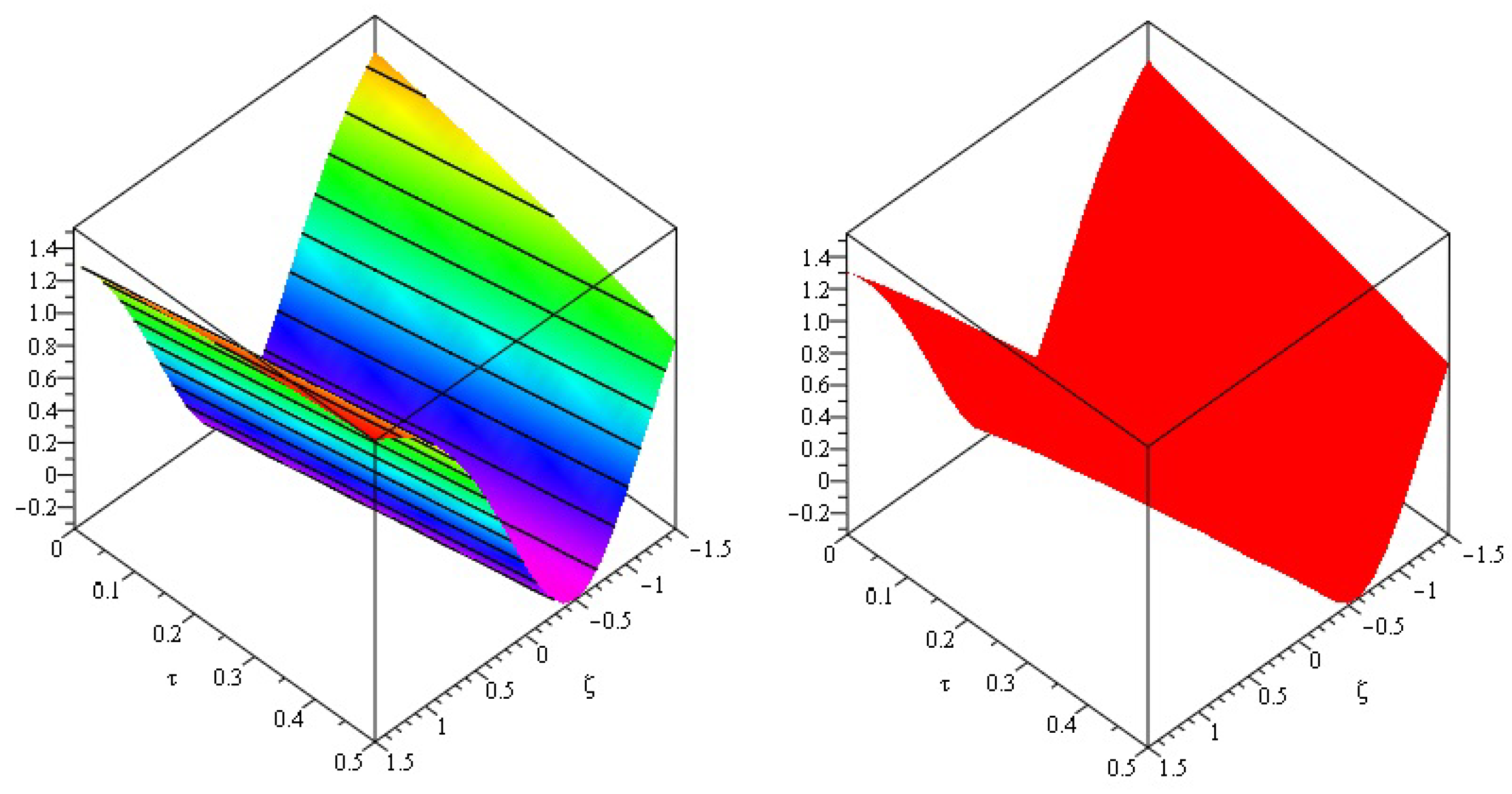
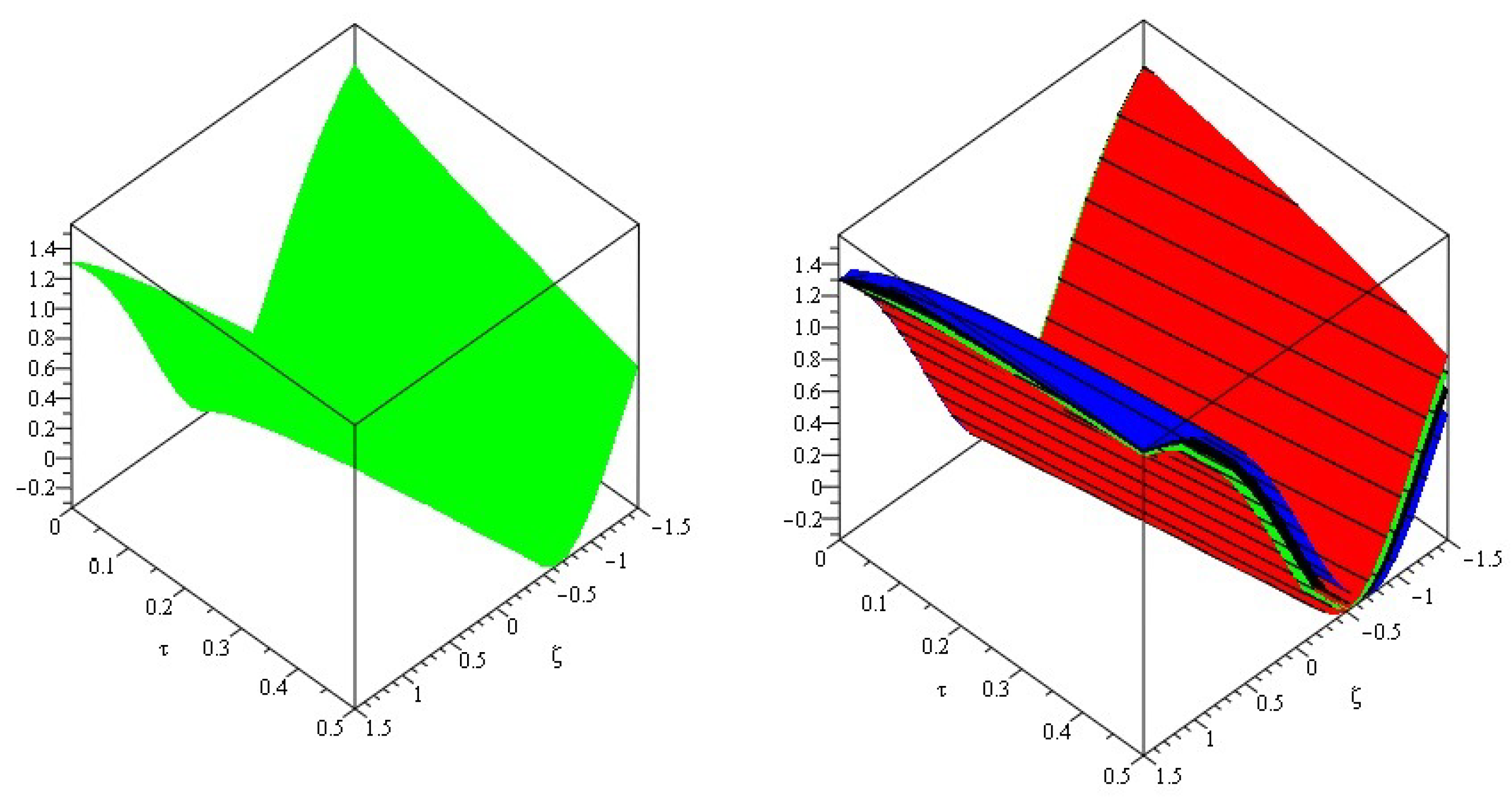
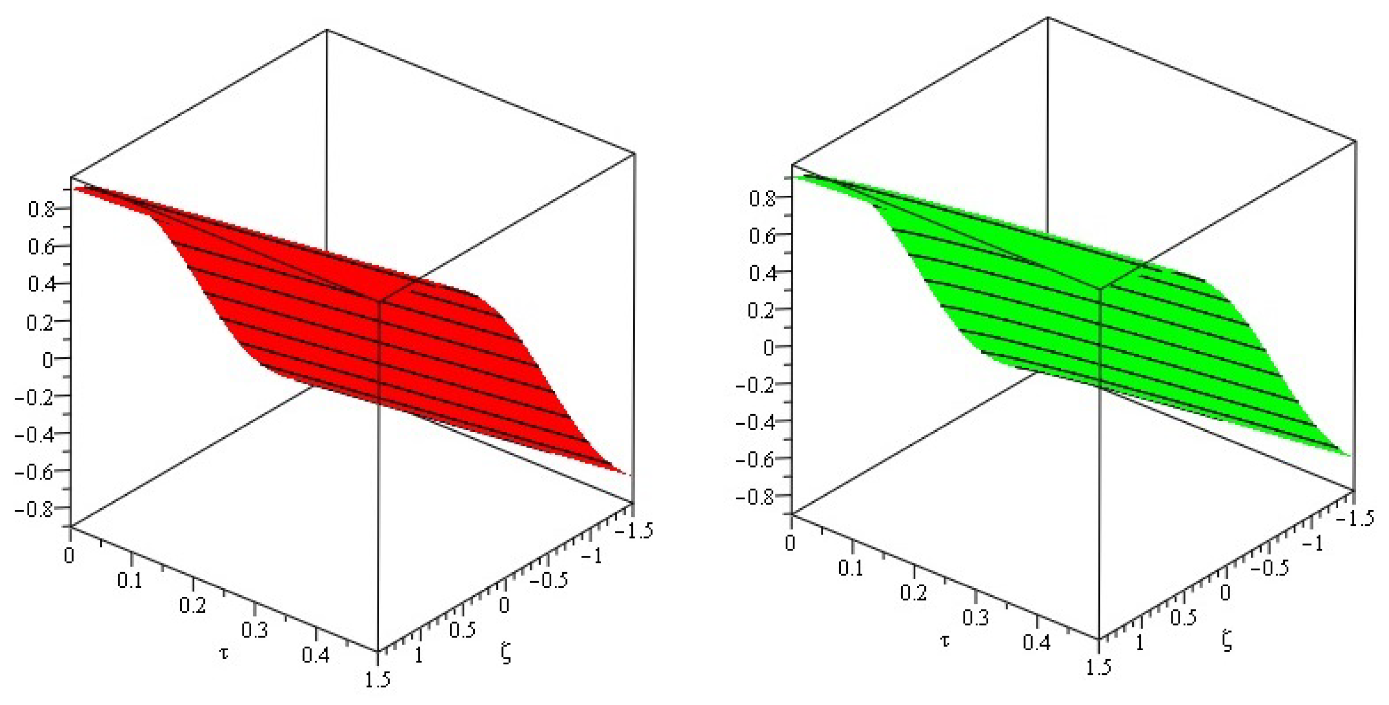
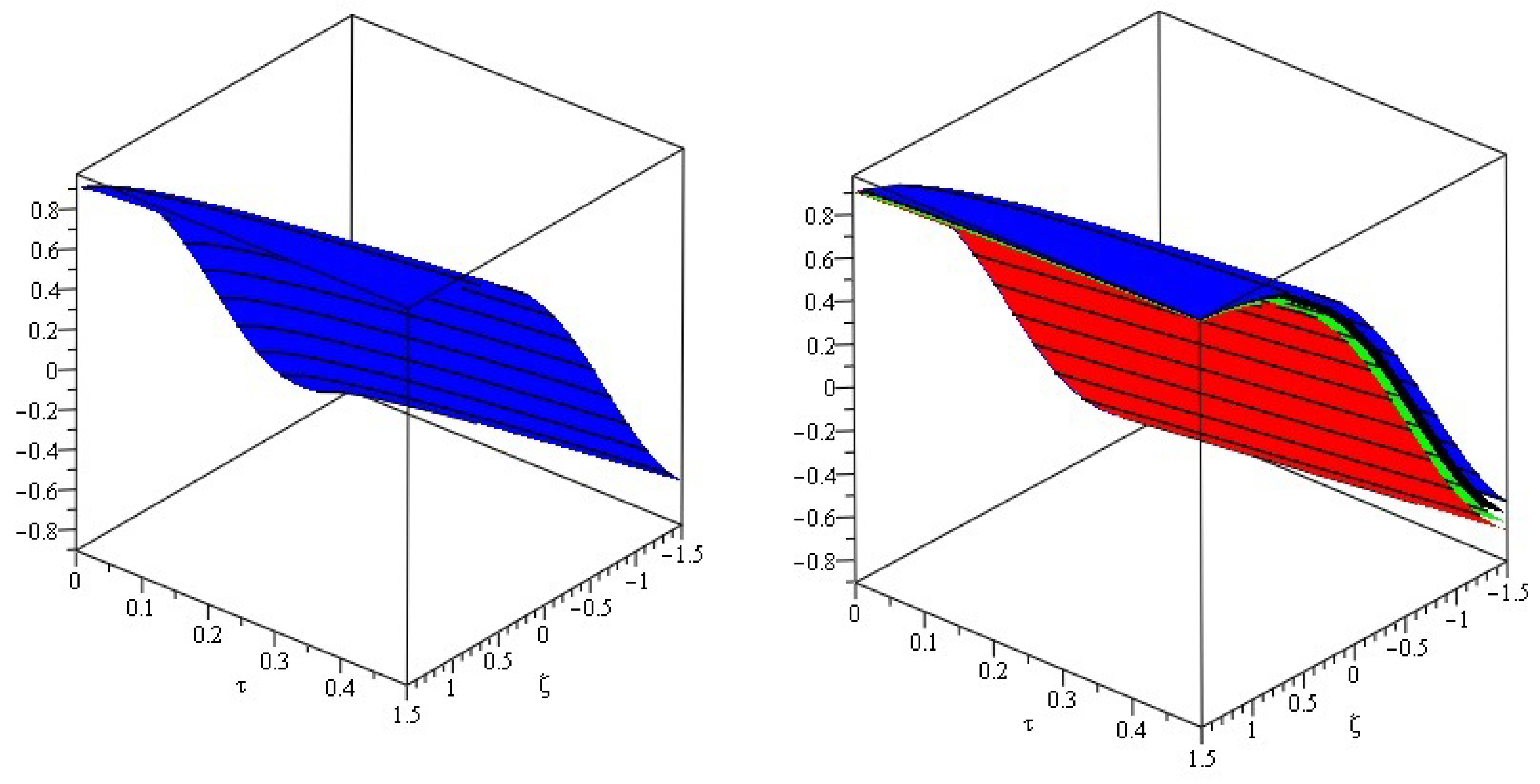
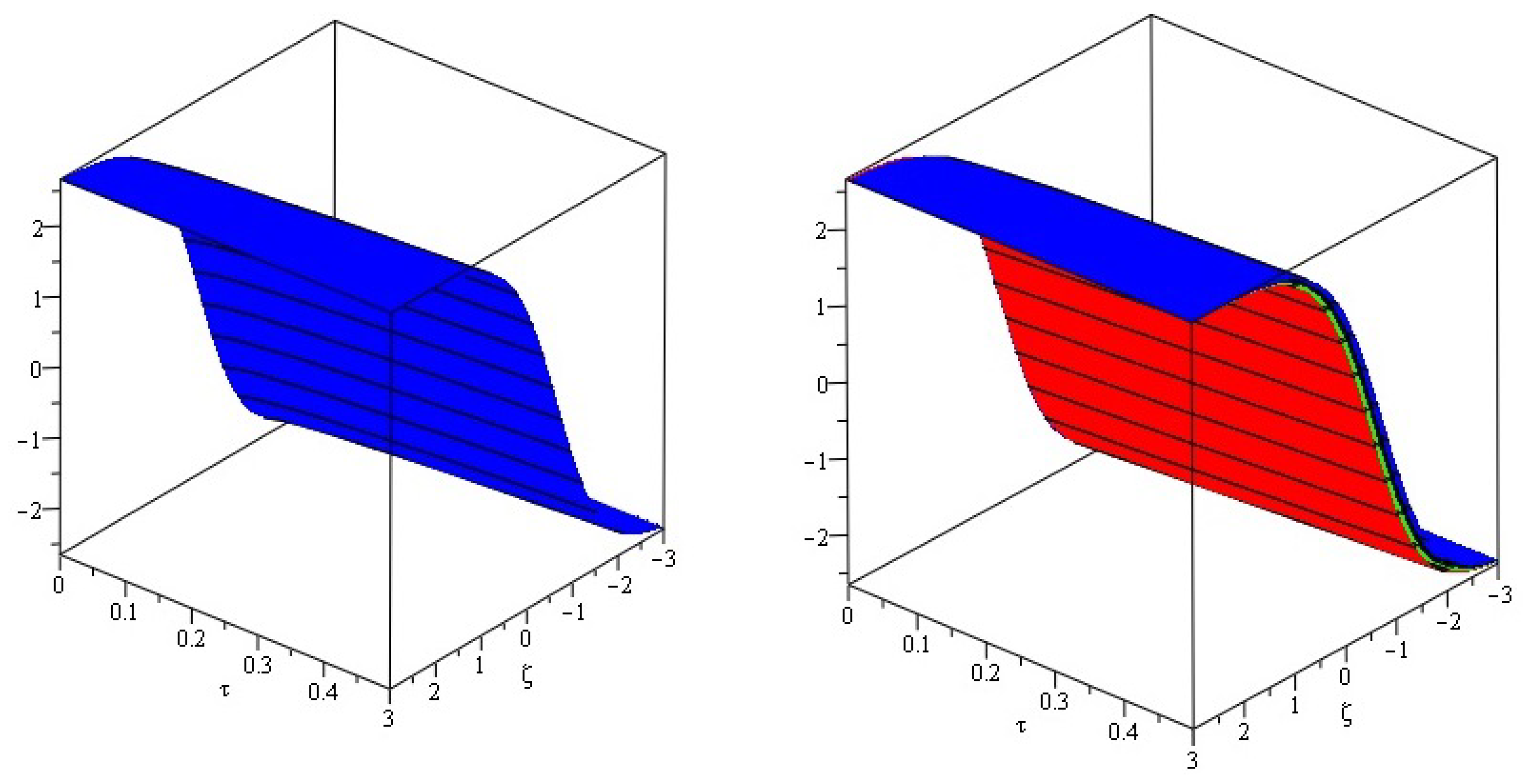
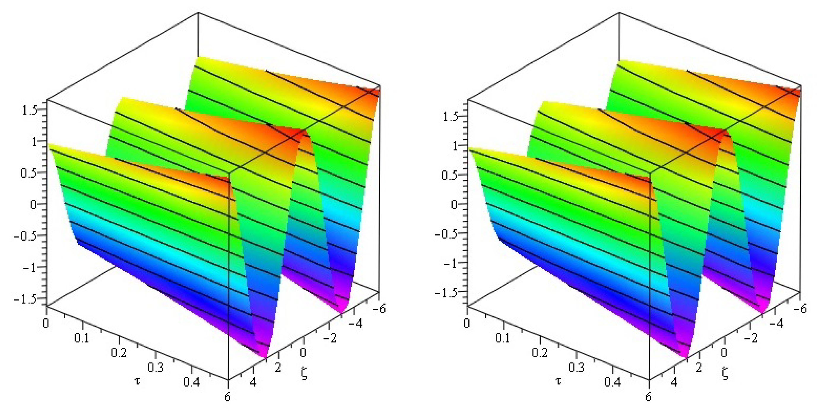
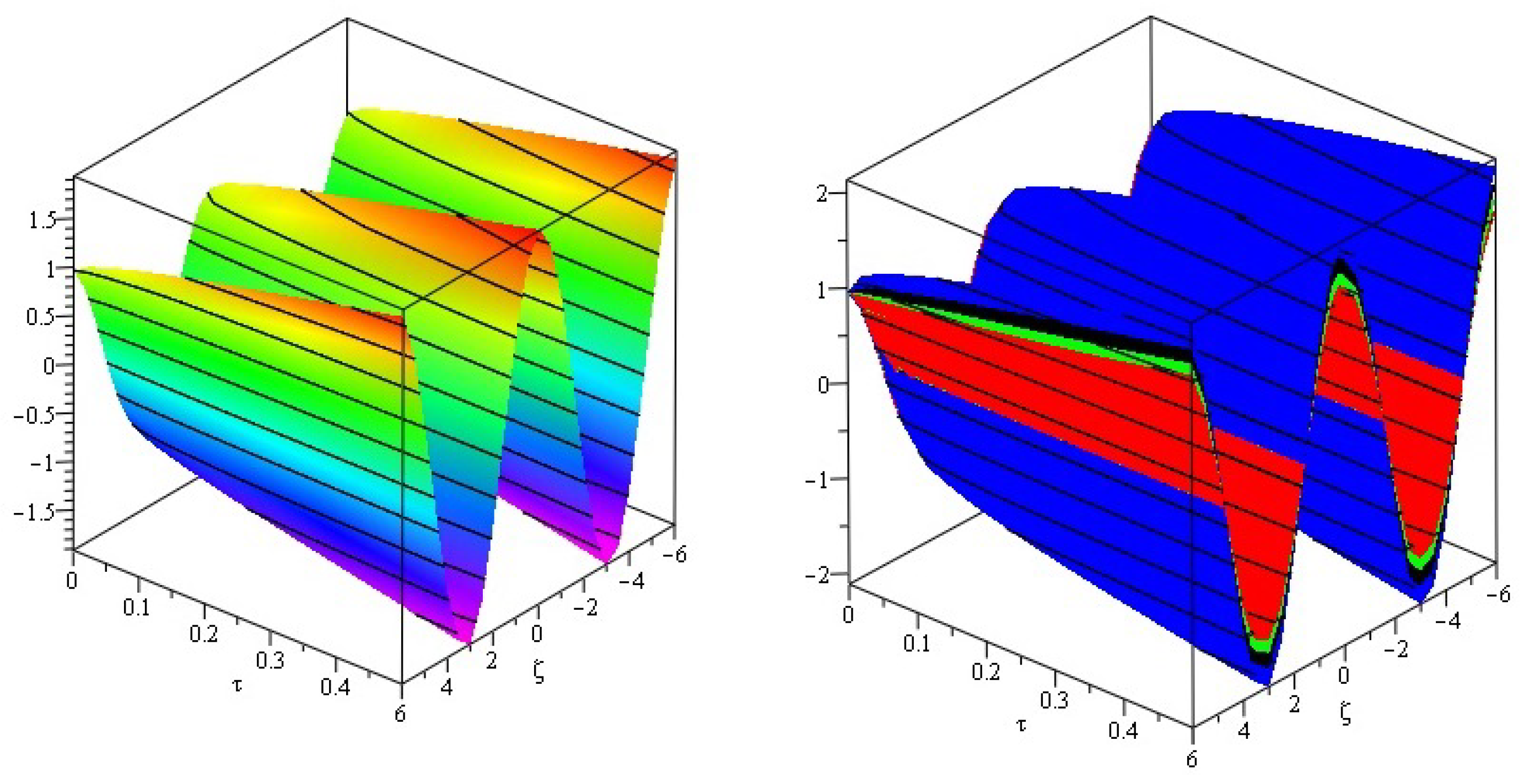
In Figure 1, the first graph shows the actual and analytic solutions and the second graph the fractional-order $\varrho =0.8$ for $\upsilon (\phi ,\wp )$ of problem 5.1. Figure 2, the first graph shows the analytic solution fractional-order at $\varrho =0.6$ and the different fractional-order $\varrho$ for $\upsilon (\phi ,\wp )$ of problem 5.1. Similarly, Figure 3, Figure 4, Figure 5 and Figure 6 shows the actual and analytic solutions and the fractional-order $\varrho$ with $\varphi (\phi ,\wp )$ and $\ell (\phi ,\wp )$ of problem 5.1.

5.2. Problem

Consider the fractional one-dimensional system Burgers equation

$$\begin{array}{cc}\hfill & \frac{{}^{ABC}{\partial }^{\varrho }\upsilon }{\partial {\wp }^{\varrho }}=\frac{{\partial }^2\upsilon }{\partial {\phi }^2}+2\upsilon \frac{\partial \upsilon }{\partial \phi }-\frac{\partial }{\partial \phi }\left(\upsilon \varphi \right),\hfill \\ \hfill & \frac{{}^{ABC}{\partial }^{\varrho }\varphi }{\partial {\wp }^{\varrho }}=\frac{{\partial }^2\varphi }{\partial {\phi }^2}+2\varphi \frac{\partial \varphi }{\partial \phi }-\frac{\partial }{\partial \phi }\left(\upsilon \varphi \right),0<\varrho \le 1,\hfill \end{array}$$

(37)

with the initial source

$$\upsilon (\phi ,0)=cos\phi ,\varphi (\phi ,0)=cos\phi .$$

Taking the Elzaki transform of (37), we have

$$\begin{array}{cc}\hfill & \frac{N\left(\varrho \right)}{\varrho {\omega }^{\varrho }+1-\varrho }\mathcal{E}\left[\upsilon (\phi ,\wp )\right]-\omega \upsilon (\phi ,0)=\mathcal{E}\left[\frac{{\partial }^2\upsilon }{\partial {\phi }^2}+2\upsilon \frac{\partial \upsilon }{\partial \phi }-\frac{\partial }{\partial \phi }\left(\upsilon \varphi \right)\right],\hfill \\ \hfill & \frac{N\left(\varrho \right)}{\varrho {\omega }^{\varrho }+1-\varrho }\mathcal{E}\left[\varphi (\phi ,\wp )\right]-\omega \varphi (\phi ,0)=\mathcal{E}\left[\frac{{\partial }^2\varphi }{\partial {\phi }^2}+2\varphi \frac{\partial \varphi }{\partial \phi }-\frac{\partial }{\partial \phi }\left(\upsilon \varphi \right)\right].\hfill \end{array}$$

(38)

Applying the Elzaki transform, we have

$$\begin{array}{cc}\hfill & \upsilon (\phi ,\wp )=cos\phi +{\mathcal{E}}^{-1}\left[\left(\frac{\varrho {\omega }^{\varrho }+1-\varrho }{N\left(\varrho \right)}\right)\mathcal{E}\left[\frac{{\partial }^2\upsilon }{\partial {\phi }^2}+2\upsilon \frac{\partial \upsilon }{\partial \phi }-\frac{\partial }{\partial \phi }\left(\upsilon \varphi \right)\right]\right],\hfill \\ \hfill & \varphi (\phi ,\wp )=cos\phi +{\mathcal{E}}^{-1}\left[\left(\frac{\varrho {\omega }^{\varrho }+1-\varrho }{N\left(\varrho \right)}\right)\mathcal{E}\left[\frac{{\partial }^2\varphi }{\partial {\phi }^2}+2\varphi \frac{\partial \varphi }{\partial \phi }-\frac{\partial }{\partial \phi }\left(\upsilon \varphi \right)\right]\right].\hfill \end{array}$$

(39)

Suppose that the results, $\upsilon (\phi ,\wp )$ and $\varphi (\phi ,\wp )$, in the form of the infinite series, are given by

$$\upsilon (\phi ,\wp )=\sum _{j=0}^{\infty }{\upsilon }_j(\phi ,\wp ),\varphi (\phi ,\wp )=\sum _{j=0}^{\infty }{\varphi }_j(\phi ,\wp ).$$

(40)

where $\upsilon {\upsilon }_{\phi }={\sum }_{j=0}^{\infty }{\mathcal{A}}_j$, ${\left(\upsilon \varphi \right)}_{\phi }={\sum }_{j=0}^{\infty }{\mathcal{B}}_j$ and $\varphi {\varphi }_{\phi }={\sum }_{j=0}^{\infty }{\mathcal{C}}_j$ are the so-called Adomian polynomials that represent the nonlinear terms, and so Equation (41) is rewritten as

$$\begin{array}{cc}\hfill & \sum _{j=0}^{\infty }{\upsilon }_j(\phi ,\wp )=cos\phi +{\mathcal{E}}^{-1}\left[\left(\frac{\varrho {\omega }^{\varrho }+1-\varrho }{N\left(\varrho \right)}\right)\mathcal{E}\left[\frac{{\partial }^2\upsilon }{\partial {\phi }^2}+2\sum _{j=0}^{\infty }{\mathcal{A}}_j-\sum _{j=0}^{\infty }{\mathcal{B}}_j\right]\right],\hfill \\ \hfill & \sum _{j=0}^{\infty }{\varphi }_j(\phi ,\wp )=cos\phi +{\mathcal{E}}^{-1}\left[\left(\frac{\varrho {\omega }^{\varrho }+1-\varrho }{N\left(\varrho \right)}\right)\mathcal{E}\left[\frac{{\partial }^2\varphi }{\partial {\phi }^2}+\sum _{j=0}^{\infty }{\mathcal{C}}_j-\sum _{j=0}^{\infty }{\mathcal{B}}_j\right]\right].\hfill \end{array}$$

(41)

The nonlinear functions by the Adomian polynomial is given as in Equation (7),

$$\begin{array}{cc}\hfill & {\mathcal{A}}_0={\upsilon }_0{\upsilon }_{0\phi },{\mathcal{A}}_1={\upsilon }_1{\upsilon }_{0\phi }+{\upsilon }_0{\upsilon }_{1\phi },{\mathcal{A}}_2={\upsilon }_2{\upsilon }_{0\phi }+{\upsilon }_1{\upsilon }_{1\phi }+{\upsilon }_0{\upsilon }_{2\phi },\hfill \\ \hfill & {\mathcal{B}}_0={\upsilon }_0{\varphi }_{0\phi }+{\varphi }_0{\upsilon }_{0\phi },{\mathcal{B}}_1=({\upsilon }_0{\varphi }_{0\phi }+{\upsilon }_1{\varphi }_{0\phi })+({\varphi }_1{\upsilon }_{0\phi }+{\varphi }_0{\upsilon }_{1\phi }),\hfill \\ \hfill & {\mathcal{B}}_2=({\upsilon }_2{\varphi }_{0\phi }+{\upsilon }_1{\varphi }_{1\phi }+{\upsilon }_0{\varphi }_{2\phi })+({\varphi }_2{\upsilon }_{0\phi }+{\varphi }_1{\upsilon }_{1\phi }+{\varphi }_0{\upsilon }_{2\phi }),\hfill \\ \hfill & {\mathcal{C}}_0={\varphi }_0{\varphi }_{0\phi },{\mathcal{C}}_1={\varphi }_1{\varphi }_{0\phi }+{\varphi }_0{\varphi }_{1\phi },{\mathcal{C}}_2={\varphi }_2{\varphi }_{0\phi }+{\varphi }_1{\varphi }_{1\phi }+{\varphi }_0{\varphi }_{2\phi }.\hfill \end{array}$$

(42)

When comparing both sides of Equation (42)

$$\begin{array}{cc}\hfill & {\upsilon }_0(\phi ,\wp )=cos\phi ,\hfill \\ \hfill & {\varphi }_0(\phi ,\wp )=cos\phi .\hfill \end{array}$$

For $j=0$

$$\begin{array}{cc}\hfill & {\upsilon }_1(\phi ,\wp )=-cos\phi \left\{\frac{\varrho {\wp }^{\varrho }}{\Gamma (\varrho +1)}+(1-\varrho )\right\},\hfill \\ \hfill & {\varphi }_1(\phi ,\wp )=-cos\phi \left\{\frac{\varrho {\wp }^{\varrho }}{\Gamma (\varrho +1)}+(1-\varrho )\right\}.\hfill \end{array}$$

For $m=1$

$$\begin{array}{cc}\hfill & {\upsilon }_2(\phi ,\wp )=cos\phi \left[\frac{{\varrho }^2{\wp }^{2\varrho }}{\Gamma (2\varrho +1)}+2\varrho (1-\varrho )\frac{{\wp }^{\varrho }}{\Gamma (\varrho +1)}+{(1-\varrho )}^2\right],\hfill \\ \hfill & {\varphi }_2(\phi ,\wp )=cos\phi \left[\frac{{\varrho }^2{\wp }^{2\varrho }}{\Gamma (2\varrho +1)}+2\varrho (1-\varrho )\frac{{\wp }^{\varrho }}{\Gamma (\varrho +1)}+{(1-\varrho )}^2\right].\hfill \end{array}$$

The analytical result of the series is given as

$$\begin{array}{cc}\hfill & \upsilon (\phi ,\wp )=\sum _{j=0}^{\infty }{\upsilon }_j(\phi ,\wp )={\upsilon }_0(\phi ,\wp )+{\upsilon }_1(\phi ,\wp )+{\upsilon }_2(\phi ,\wp )+\cdots .\hfill \\ \hfill & \varphi (\phi ,\wp )=\sum _{j=0}^{\infty }{\varphi }_j(\phi ,\wp )={\varphi }_0(\phi ,\wp )+{\varphi }_1(\phi ,\wp )+{\varphi }_2(\phi ,\wp )+\cdots .\hfill \end{array}$$

$$\begin{array}{cc}\hfill & \upsilon (\phi ,\wp )=cos\phi -cos\phi \left\{\frac{\varrho {\wp }^{\varrho }}{\Gamma (\varrho +1)}+(1-\varrho )\right\}+cos\phi \left[\frac{{\varrho }^2{\wp }^{2\varrho }}{\Gamma (2\varrho +1)}+2\varrho (1-\varrho )\frac{{\wp }^{\varrho }}{\Gamma (\varrho +1)}+{(1-\varrho )}^2\right]+\cdots .\hfill \\ \hfill & \varphi (\phi ,\wp )=cos\phi -cos\phi \left\{\frac{\varrho {\wp }^{\varrho }}{\Gamma (\varrho +1)}+(1-\varrho )\right\}+cos\phi \left[\frac{{\varrho }^2{\wp }^{2\varrho }}{\Gamma (2\varrho +1)}+2\varrho (1-\varrho )\frac{{\wp }^{\varrho }}{\Gamma (\varrho +1)}+{(1-\varrho )}^2\right]+\cdots .\hfill \end{array}$$

The exact result is by putting $\varrho =1$

$$\begin{array}{cc}\hfill & \upsilon (\phi ,\wp )=cos\phi (1-\wp +\frac{{\wp }^2}{2}-\cdots ),\hfill \\ \hfill & \varphi (\phi ,\wp )=cos\phi (1-\wp +\frac{{\wp }^2}{2}-\cdots ).\hfill \end{array}$$

(43)

The exact result is $\upsilon (\phi ,\wp )=cos\left(\phi \right){exp}^{-\wp }$ and $\varphi (\phi ,\wp )=cos\left(\phi \right){exp}^{-\wp }.$

VITM analytic solutions:

For Equation (39), we have the iterative technique

$$\begin{array}{cc}\hfill & {\upsilon }_{j+1}(\phi ,\wp )={\upsilon }_j(\phi ,\wp )-{\mathcal{E}}^{-1}\left[\left(\frac{\varrho {\omega }^{\varrho }+1-\varrho }{N\left(\varrho \right)}\right)\mathcal{E}\left\{\frac{{\partial }^2{\upsilon }_j}{\partial {\phi }^2}+2{\upsilon }_j\frac{\partial {\upsilon }_j}{\partial \phi }-\frac{\partial }{\partial \phi }\left({\upsilon }_j{\varphi }_j\right)\right\}\right],\hfill \\ \hfill & {\varphi }_{j+1}(\phi ,\wp )={\varphi }_j(\phi ,\wp )-{\mathcal{E}}^{-1}\left[\left(\frac{\varrho {\omega }^{\varrho }+1-\varrho }{N\left(\varrho \right)}\right)\mathcal{E}\left\{\frac{{\partial }^2{\varphi }_j}{\partial {\phi }^2}+2{\varphi }_j\frac{\partial \varphi }{\partial \phi }-\frac{\partial }{\partial \phi }\left({\upsilon }_j{\varphi }_j\right)\right\}\right],\hfill \end{array}$$

(44)

where

$$\begin{array}{cc}\hfill & {\upsilon }_0(\phi ,\wp )=cos\phi ,\hfill \\ \hfill & {\varphi }_0(\phi ,\wp )=cos\phi .\hfill \end{array}$$

For $j=0,1,2,\cdots$

$$\begin{array}{cc}\hfill & {\upsilon }_1(\phi ,\wp )={\upsilon }_0(\phi ,\wp )-{\mathcal{E}}^{-1}\left[\left(\frac{\varrho {\omega }^{\varrho }+1-\varrho }{N\left(\varrho \right)}\right)\mathcal{E}\left\{\frac{{\partial }^2{\upsilon }_0}{\partial {\phi }^2}+2{\upsilon }_0\frac{\partial {\upsilon }_0}{\partial \phi }-\frac{\partial }{\partial \phi }\left({\upsilon }_0{\varphi }_0\right)\right\}\right],\hfill \\ \hfill & {\upsilon }_1(\phi ,\wp )=-cos\phi \left\{\frac{\varrho {\wp }^{\varrho }}{\Gamma (\varrho +1)}+(1-\varrho )\right\},\hfill \\ \hfill & {\varphi }_1(\phi ,\wp )={\varphi }_0(\phi ,\wp )-{\mathcal{E}}^{-1}\left[\left(\frac{\varrho {\omega }^{\varrho }+1-\varrho }{N\left(\varrho \right)}\right)\mathcal{E}\left\{\frac{{\partial }^2{\varphi }_0}{\partial {\phi }^2}+2{\varphi }_0\frac{\partial \varphi }{\partial \phi }-\frac{\partial }{\partial \phi }\left({\upsilon }_0{\varphi }_0\right)\right\}\right],\hfill \\ \hfill & {\varphi }_1(\phi ,\wp )=-cos\phi \left\{\frac{\varrho {\wp }^{\varrho }}{\Gamma (\varrho +1)}+(1-\varrho )\right\},\hfill \end{array}$$

(45)

$$\begin{array}{cc}\hfill & {\upsilon }_2(\phi ,\wp )={\upsilon }_1(\phi ,\wp )-{\mathcal{E}}^{-1}\left[\left(\frac{\varrho {\omega }^{\varrho }+1-\varrho }{N\left(\varrho \right)}\right)\mathcal{E}\left\{\frac{{\partial }^2{\upsilon }_1}{\partial {\phi }^2}+2{\upsilon }_1\frac{\partial {\upsilon }_1}{\partial \phi }-\frac{\partial }{\partial \phi }\left({\upsilon }_1{\varphi }_1\right)\right\}\right],\hfill \\ \hfill & {\upsilon }_2(\phi ,\wp )=cos\phi \left[\frac{{\varrho }^2{\wp }^{2\varrho }}{\Gamma (2\varrho +1)}+2\varrho (1-\varrho )\frac{{\wp }^{\varrho }}{\Gamma (\varrho +1)}+{(1-\varrho )}^2\right],\hfill \\ \hfill & {\varphi }_2(\phi ,\wp )={\varphi }_1(\phi ,\wp )-{\mathcal{E}}^{-1}\left[\left(\frac{\varrho {\omega }^{\varrho }+1-\varrho }{N\left(\varrho \right)}\right)\mathcal{E}\left\{\frac{{\partial }^2{\varphi }_1}{\partial {\phi }^2}+2{\varphi }_1\frac{\partial \varphi }{\partial \phi }-\frac{\partial }{\partial \phi }\left({\upsilon }_1{\varphi }_1\right)\right\}\right],\hfill \\ \hfill & {\varphi }_1(\phi ,\wp )=cos\phi \left[\frac{{\varrho }^2{\wp }^{2\varrho }}{\Gamma (2\varrho +1)}+2\varrho (1-\varrho )\frac{{\wp }^{\varrho }}{\Gamma (\varrho +1)}+{(1-\varrho )}^2\right],\hfill \end{array}$$

(46)

$$\begin{array}{cc}\hfill & \upsilon (\phi ,\wp )=cos\phi -cos\phi \left\{\frac{\varrho {\wp }^{\varrho }}{\Gamma (\varrho +1)}+(1-\varrho )\right\}+cos\phi \left[\frac{{\varrho }^2{\wp }^{2\varrho }}{\Gamma (2\varrho +1)}+2\varrho (1-\varrho )\frac{{\wp }^{\varrho }}{\Gamma (\varrho +1)}+{(1-\varrho )}^2\right]+\cdots .\hfill \\ \hfill & \varphi (\phi ,\wp )=cos\phi -cos\phi \left\{\frac{\varrho {\wp }^{\varrho }}{\Gamma (\varrho +1)}+(1-\varrho )\right\}+cos\phi \left[\frac{{\varrho }^2{\wp }^{2\varrho }}{\Gamma (2\varrho +1)}+2\varrho (1-\varrho )\frac{{\wp }^{\varrho }}{\Gamma (\varrho +1)}+{(1-\varrho )}^2\right]+\cdots .\hfill \end{array}$$

We achieve the exact solution by putting $\varrho =1$

$$\begin{array}{cc}\hfill & \upsilon (\phi ,\wp )=cos\phi (1-\wp +\frac{{\wp }^2}{2}-\cdots ),\hfill \\ \hfill & \varphi (\phi ,\wp )=cos\phi (1-\wp +\frac{{\wp }^2}{2}-\cdots ).\hfill \end{array}$$

(47)

The exact result is $\upsilon (\phi ,\wp )=cos\left(\phi \right){exp}^{-\wp }$ and $\varphi (\phi ,\wp )=cos\left(\phi \right){exp}^{-\wp }$

In Figure 7, the first graph shows the actual and analytic solutions, and the second graph the fractional-order $\varrho =0.8$ for $\upsilon (\phi ,\wp )$ of problem 5.2. In Figure 8, the first graph shows the analytic solution of the fractional-order at $\varrho =0.6$ and the different fractional-order $\varrho$ for $\upsilon (\phi ,\wp )$ of problem 5.2.

6. Conclusions

The coupled nonlinear PDEs were defined by applying the EDM and VITM. When the results of these approaches are compared to the actual solution, it is clear that the provided methods are incredibly basic and straightforward to deal with the nonlinear terms. The results obtained formed a series that gradually tended to the precise exact solution. By solving four nonlinear systems, it is shown that the proposed methods become very close to the exact solution. It has been verified that the suggested approaches require less computing labour, resulting in quick convergence. Furthermore, EDM and VITM are particularly productive and competitive in finding approximate analytic solutions to a broad variety of real-world engineering and scientific problems.

References

- Nonlaopon, K.; Naeem, M.; Zidan, A.M.; Alsanad, A.; Gumaei, A. Numerical investigation of the time-fractional Whitham-Broer-Kaup equation involving without singular kernel operators. Complexity 2021, 7979365. [Google Scholar] [CrossRef]
- Caputo, M. Linear models of dissipation whose Q is almost frequency independent-II. Geophys. J. Int. 1967, 13, 529–539. [Google Scholar] [CrossRef]
- Caputo, M.; Fabrizio, M. A new definition of fractional derivative without singular kernel. Progr. Fract. Differ. Appl. 2015, 1, 1–13. [Google Scholar]
- Iqbal, N.; Yasmin, H.; Ali, A.; Bariq, A.; Al-Sawalha, M.M.; Mohammed, W.W. Numerical Methods for Fractional-Order Fornberg-Whitham Equations in the Sense of Atangana-Baleanu Derivative. J. Funct. Spaces 2021, 2021, 2197247. [Google Scholar] [CrossRef]
- Iqbal, N.; Yasmin, H.; Rezaiguia, A.; Kafle, J.; Almatroud, A.O.; Hassan, T.S. Analysis of the Fractional-Order Kaup–Kupershmidt Equation via Novel Transforms. J. Math. 2021, 2021, 2567927. [Google Scholar] [CrossRef]
- Areshi, M.; Khan, A.; Shah, R.; Nonlaopon, K. Analytical investigation of fractional-order Newell-Whitehead-Segel equations via a novel transform. AIMS Math. 2022, 7, 6936–6958. [Google Scholar] [CrossRef]
- Bagley, R.L.; Torvik, P.J. A theoretical basis for the application of fractional calculus to viscoelasticity. J. Rheol. 1983, 27, 201–210. [Google Scholar] [CrossRef]
- Baillie, R.T. Long memory processes and fractional integration in econometrics. J. Econom. 1996, 73, 5–59. [Google Scholar] [CrossRef]
- Chow, T.S. Fractional dynamics of interfaces between soft-nanoparticles and rough substrates. Phys. Lett. A 2005, 342, 148–155. [Google Scholar] [CrossRef]
- Chen, C.M.; Liu, F.; Anh, V.; Turner, I. Numerical methods for solving a two-dimensional variable-order anomalous subdiffusion equation. Math. Comput. 2012, 81, 345–366. [Google Scholar] [CrossRef]
- Shah, N.A.; Alyousef, H.A.; El-Tantawy, S.A.; Shah, R.; Chung, J.D. Analytical Investigation of Fractional-Order Korteweg-De-Vries-Type Equations under Atangana-Baleanu-Caputo Operator: Modeling Nonlinear Waves in a Plasma and Fluid. Symmetry 2022, 14, 739. [Google Scholar] [CrossRef]
- Kilbas, A.A.; Srivastava, H.M.; Trujillo, J.J. Theory and Applications of Fractional Differential Equations; Elsevier: Amsterdam, The Netherlands, 2006; Volume 204. [Google Scholar]
- Podlubny, I. Fractional Differential Equations; Academic Press: San Diego, CA, USA, 1999; p. 198. [Google Scholar]
- Inc, M. The approximate and exact solutions of the space-and time-fractional Burgers equations with initial conditions by variational iteration method. J. Math. Anal. Appl. 2008, 345, 476–484. [Google Scholar] [CrossRef] [Green Version]
- Samko, S.G.; Kilbas, A.A.; Marichev, O.I. Fractional Integrals and Derivatives; Translated from the 1987 Russian Original; Gordon and Breach: New York, NY, USA, 1993. [Google Scholar]
- Shah, N.A.; Hamed, Y.S.; Abualnaja, K.M.; Chung, J.D.; Khan, A. A comparative analysis of fractional-order kaup-kupershmidt equation within different operators. Symmetry 2022, 14, 986. [Google Scholar] [CrossRef]
- Agrawal, O.P.; Defterli, O.; Baleanu, D. Fractional optimal control problems with several state and control variables. J. Vib. Control 2010, 16, 1967–1976. [Google Scholar] [CrossRef]
- Sunthrayuth, P.; Ullah, R.; Khan, A.; Shah, R.; Kafle, J.; Mahariq, I.; Jarad, F. Numerical analysis of the fractional-order nonlinear system of Volterra integro-differential equations. J. Funct. Spaces 2021, 2021, 1537958. [Google Scholar] [CrossRef]
- Aljahdaly, N.H.; Akgul, A.; Shah, R.; Mahariq, I.; Kafle, J. A comparative analysis of the fractional-order coupled Korteweg-De Vries equations with the Mittag-Leffler law. J. Math. 2022, 2022, 8876149. [Google Scholar] [CrossRef]
- Sunthrayuth, P.; Aljahdaly, N.H.; Ali, A.; Shah, R.; Mahariq, I.; Tchalla, A.M. ψ-Haar Wavelet Operational Matrix Method for Fractional Relaxation-Oscillation Equations Containing-Caputo Fractional Derivative. J. Funct. Spaces 2021, 2021, 7117064. [Google Scholar] [CrossRef]
- Mukhtar, S.; Shah, R.; Noor, S. The Numerical Investigation of a Fractional-Order Multi-Dimensional Model of Navier-Stokes Equation via Novel Techniques. Symmetry 2022, 14, 1102. [Google Scholar] [CrossRef]
- Alesemi, M.; Iqbal, N.; Hamoud, A.A. The analysis of fractional-order proportional delay physical models via a novel transform. Complexity 2022, 2022, 2431533. [Google Scholar] [CrossRef]
- Alesemi, M.; Iqbal, N.; Botmart, T. Novel analysis of the fractional-order system of non-linear partial differential equations with the exponential-decay kernel. Mathematics 2022, 10, 615. [Google Scholar] [CrossRef]
- Wu, J. Theory and Applications of Partial Functional Differential Equations; Springer Science & Business Media: Berlin/Heidelberg, Germany, 1996; Volume 119. [Google Scholar]
- Yang, X.J.; Baleanu, D. Fractal heat conduction problem solved by local fractional variation iteration method. Therm. Sci. 2013, 17, 625–628. [Google Scholar] [CrossRef]
- Qin, Y.; Khan, A.; Ali, I.; Al Qurashi, M.; Khan, H.; Shah, R.; Baleanu, D. An efficient analytical approach for the solution of certain fractional-order dynamical systems. Energies 2020, 13, 2725. [Google Scholar] [CrossRef]
- Mirmoradia, S.H.; Hosseinpoura, I.; Ghanbarpour, S.; Barari, A. Application of an approximate analytical method to nonlinear Troesch’s problem. Appl. Math. Sci. 2009, 3, 1579–1585. [Google Scholar]
- Kumar, A.; Kumar, S.; Yan, S.P. Residual power series method for fractional diffusion equations. Fundam. Inform. 2017, 151, 213–230. [Google Scholar] [CrossRef]
- Khan, H.; Khan, A.; Al-Qurashi, M.; Shah, R.; Baleanu, D. Modified modelling for heat like equations within Caputo operator. Energies 2020, 13, 2002. [Google Scholar] [CrossRef]
- Khan, H.; Khan, A.; Kumam, P.; Baleanu, D.; Arif, M. An approximate analytical solution of the Navier-Stokes equations within Caputo operator and Elzaki transform decomposition method. Adv. Diff. Equ. 2020, 2020, 1–23. [Google Scholar]
- Keskin, Y.; Oturanc, G. Reduced differential transform method for partial differential equations. Int. J. Nonlinear Sci. Numer. Simul. 2009, 10, 741–750. [Google Scholar] [CrossRef]
- Evans, D.J.; Raslan, K.R. The Adomian decomposition method for solving delay differential equation. Int. J. Comput. Math. 2005, 82, 49–54. [Google Scholar] [CrossRef]
- Bateman, H. Some recent researches on the motion of fluids. Mon. Weather. Rev. 1915, 43, 163–170. [Google Scholar] [CrossRef]
- Yasmin, H. Numerical Analysis of Time-Fractional Whitham-Broer-Kaup Equations with Exponential-Decay Kernel. Fractal Fract. 2022, 6, 142. [Google Scholar] [CrossRef]
- Rashidi, M.M.; Erfani, E. New analytical method for solving Burgers and nonlinear heat transfer equations and comparison with HAM. Comput. Phys. Commun. 2009, 180, 1539–1544. [Google Scholar] [CrossRef]
- Moslem, W.M.; Sabry, R. Zakharov-Kuznetsov-Burgers equation for dust ion acoustic waves. Chaos Solitons Fractals 2008, 36, 628–634. [Google Scholar] [CrossRef]
- Iqbal, N.; Botmart, T.; Mohammed, W.W.; Ali, A. Numerical investigation of fractional-order Kersten-Krasil’shchik coupled KdV-mKdV system with Atangana-Baleanu derivative. Adv. Contin. Discret. Models 2022, 2022, 1–20. [Google Scholar] [CrossRef]
- Liu, Z.J.; Adamu, M.Y.; Suleiman, E.; He, J.H. Hybridization of homotopy perturbation method and Laplace transformation for the partial differential equations. Therm. Sci. 2017, 21, 1843–1846. [Google Scholar] [CrossRef] [Green Version]
- Hristov, J. An exercise with the He’s variation iteration method to a fractional Bernoulli equation arising in transient conduction with non-linear heat flux at the boundary. Int. Rev. Chem. Eng. 2012, 4, 489–497. [Google Scholar]
- Liu, C.F.; Kong, S.S.; Yuan, S.J. Reconstructive schemes for variational iteration method within Yang-Laplace transform with application to fractal heat conduction problem. Therm. Sci. 2013, 17, 715–721. [Google Scholar] [CrossRef]
- Atangana, A.; Baleanu, D. New fractional derivatives with nonlocal and non-singular kernel: Theory and application to heat transfer model. Therm. Sci. 2016, 20, 763–769. [Google Scholar] [CrossRef] [Green Version]
- Elzaki, T.M. The new integral transform Elzaki transform. Glob. J. Pure Appl. Math. 2011, 7, 57–64. [Google Scholar]
- Alderremy, A.A.; Elzaki, T.M.; Chamekh, M. New transform iterative method for solving some Klein-Gordon equations. Results Phys. 2018, 10, 655–659. [Google Scholar] [CrossRef]
- Kim, H. The time shifting theorem and the convolution for Elzaki transform. Int. J. Pure Appl. Math. 2013, 87, 261–271. [Google Scholar] [CrossRef]
Figure 1.
The first graph shows the actual and analytic solutions and the second graph the fractional-order for of problem 5.1.
Figure 2.
The first graph shows the analytic solution of the fractional-order at and second figure the different fractional-order for of problem 5.1.
Figure 3.
Figure 4.
The first graph shows the analytic solution of the fractional-order at and second graph the different fractional-order for of problem 5.1.
Figure 5.
Figure 6.
Figure 7.
The first graph shows the actual and analytic solutions and the second graph the fractional-order for of problem 5.2.
Figure 8.
The first graph shows the analytic solution of the fractional-order at and second graph the different fractional-order for of problem 5.2.
Publisher’s Note: MDPI stays neutral with regard to jurisdictional claims in published maps and institutional affiliations. |
© 2022 by the authors. Licensee MDPI, Basel, Switzerland. This article is an open access article distributed under the terms and conditions of the Creative Commons Attribution (CC BY) license (https://creativecommons.org/licenses/by/4.0/).
Share and Cite
MDPI and ACS Style
Yasmin, H.; Iqbal, N. A Comparative Study of the Fractional Coupled Burgers and Hirota–Satsuma KdV Equations via Analytical Techniques. Symmetry 2022, 14, 1364. https://0-doi-org.brum.beds.ac.uk/10.3390/sym14071364
AMA Style
Yasmin H, Iqbal N. A Comparative Study of the Fractional Coupled Burgers and Hirota–Satsuma KdV Equations via Analytical Techniques. Symmetry. 2022; 14(7):1364. https://0-doi-org.brum.beds.ac.uk/10.3390/sym14071364
Chicago/Turabian StyleYasmin, Humaira, and Naveed Iqbal. 2022. "A Comparative Study of the Fractional Coupled Burgers and Hirota–Satsuma KdV Equations via Analytical Techniques" Symmetry 14, no. 7: 1364. https://0-doi-org.brum.beds.ac.uk/10.3390/sym14071364
Note that from the first issue of 2016, this journal uses article numbers instead of page numbers. See further details here.