
Generating Optimal Discrete Analogue of the Generalized Pareto Distribution under Bayesian Inference with Applications


1
Department of Basic Science, Preparatory Year Deanship, King Faisal University, Hofuf 31982, Saudi Arabia
2
Department of Statistical, Faculty of Business Administration, Delta University for Science and Technology, Gamasa 11152, Egypt
3
The Scientific Association for Studies and Applied Research, Al Manzalah 35646, Egypt
*
Author to whom correspondence should be addressed.
Symmetry 2022, 14(7), 1457; https://0-doi-org.brum.beds.ac.uk/10.3390/sym14071457
Submission received: 20 June 2022
/
Revised: 13 July 2022
/
Accepted: 14 July 2022
/
Published: 16 July 2022
(This article belongs to the Special Issue Symmetrical and Asymmetrical Distributions in Statistics and Data Science)
Abstract
:This paper studies three discretization methods to formulate discrete analogues of the well-known continuous generalized Pareto distribution. The generalized Pareto distribution provides a wide variety of probability spaces, which support threshold exceedances, and hence, it is suitable for modeling many failure time issues. Bayesian inference is applied to estimate the discrete models with different symmetric and asymmetric loss functions. The symmetric loss function being used is the squared error loss function, while the two asymmetric loss functions are the linear exponential and general entropy loss functions. A detailed simulation analysis was performed to compare the performance of the Bayesian estimation using the proposed loss functions. In addition, the applicability of the optimal discrete generalized Pareto distribution was compared with other discrete distributions. The comparison was based on different goodness-of-fit criteria. The results of the study reveal that the discretized generalized Pareto distribution is quite an attractive alternative to other discrete competitive distributions.
Keywords:
discretization methods; Bayesian estimation; symmetric and asymmetric loss functions; prior distribution; simulation analysis; Monte Carlo Markov chain; goodness-of-fit measuresMSC:
65C20; 60E05; 62P30; 62L151. Introduction
The amount of data available in nature has become larger, demanding new statistical distributions to modify the description of each phenomenon or experiment under study. Most lifetime data are continuous, while they are discrete in observation, which leads to a need for appropriate methods to discretize the continuous distribution to better fit these data. Almost always, the observed values are in fact discrete because they are restrained to only a finite number of decimal places and cannot really create all points in a continuum. In some other cases, because of the accuracy of the measuring apparatus or the need to save space, continuous variables are measured by the frequencies of separate class intervals, whose union creates the whole range of random variables, and multinomial law is used to model this situation. Therefore, considering them as discrete values is more appropriate. Even for a continuous life experiment, records in an interval of time result in a discrete model, which seems more suitable than a continuous model.
Recently, many discrete distributions have been identified, particularly in reliability and survival analyses. For a special description and the role of discrete distributions, one may refer to [1,2,3,4,5,6,7,8], among others. Hence, many authors have conducted much work to originate and develop discrete reliability theory from various points of view.
The characterization of continuous random variables can be performed either by their probability density function (pdf), cumulative distribution function (CDF), moments, hazard rate functions, or others. Usually, creating a discrete analogue from a continuous distribution is based on the principle of preserving one or more characteristic properties of the continuous one. Consequently, different ways to discretize a continuous distribution appear in the literature, depending on the property the researcher aims to preserve (see, for example, [9,10]). In [11], the author provided an extensive survey of different discretization methods that preserve different functions.
There are many useful tips for creating discrete random variables from continuous ones: through discretization, data can actually be summarized and simplified; in addition, they can also become easier to understand, use, and explain for researchers (see [12]). Other tests appearing in the literature are suitable for both discrete and continuous distributions (see, for example, [13,14]).
Therefore, it is desirable to study a suitable discrete distribution created from the underlying continuous models.
In the present paper, we discretize the continuous generalized Pareto distribution (GPD) using three different discretization methods. Almost all authors have used one discretization method, which depends on the survival function. In [6,7], discrete normal and discrete Rayleigh distributions were introduced, respectively, and the author used the survival discretization approach. Using the same approach, discrete Burr type II was studied in [15]. Additionally, [16] introduced the discrete additive Weibull distribution (see also [17,18,19,20,21,22,23]). However, there remains a need to improve discrete models and generate new ones for the sake of describing and fitting the huge amount of data that appear and spread evenly throughout humans’ daily lives. Further, [24] discussed the discrete odd Perks-G class of distributions. Reference [25] introduced a new novel discrete distribution with an application to COVID-19, and [26] obtained a discrete Weibull Marshall–Olkin family of distributions.
We aim to discretize the GPD since it has extensive applications and can model many real-life distributions. Recently, many authors have studied the continuous GPD; for example, one may refer to [27], in which the authors discussed baseline methods for parameter estimation. The authors of [28] performed statistical inference of the dynamic conditional GPD with weather and air quality factors, and [29] discussed outlier-robust truncated maximum likelihood parameter estimators of the GPD. Reference [30] introduced risk analysis using the GPD.
The originality of this work stems from the fact that no earlier research has been conducted in this area using the suggested discretization method and compared it with other methods from a Bayesian point of view. Symmetric and asymmetric loss functions are performed in the Bayesian estimation method using different parameter values. Therefore, the main objective of this paper is to illustrate the efficiency and performance of discrete generalized Pareto distributions (DGPDs) for modeling different COVID-19 daily death cases.
The rest of this paper is organized as follows: Section 2 contains the model description and the discretization methods. Section 3 presents Bayesian inference for unknown parameters, and both point and interval estimations are performed for the three DGPDs. In Section 4, the simulation study is described. Real data examples are provided in Section 5. Finally, conclusions are provided in Section 6.
2. Model Description and Discretization Methods
The generalized Pareto distribution is a continuous distribution with two parameters. However, its continuous distributional form is limited in characterizing data of discrete forms. Discretizing the GPD, therefore, produces a consequent distribution that accommodates count data while preserving the vital tail-modeling feature of the GPD. In this paper, we perform three discrete versions of the two-parameter GPD and use these counterparts to model real-life data.
The probability density function (pdf) of the continuous GPD is given as
and the cumulative distribution function (CDF) is given by
where > 0 is the scale parameter, and is the shape parameter, . The domain of the random variable depends on the value of , particularly whether it is positive or negative; hence, we have two cases: first, when > 0, , and when < 0, the support of x will be bounded, i.e., . For > 0, the GPD is the well-known Pareto distribution. When , the GPD reduces to the exponential distribution, as shown in Equation (1).
The GPD has a mean of (/(1 − )) and a variance , provided < 0.5. The survival function and the hazard rate function HR are given, respectively, as follows:
and
The three discretization methods are presented in the next subsections. The first method aims to preserve the survival function, while the second method preserves the pdf, and the third method preserves the hazard rate.
2.1. Survival Discretization Method
The probability mass function (pmf) of a discrete distribution is defined by [6,7] as follows:
where is the survival function given by Equation (3). Hence, the pmf of the first discrete generalized Pareto distribution (DGPD1) is
The CDF of the DGPD1 distribution in the survival discretization method can be written as:
2.2. Methodology II
In this method, the pmf of the discrete random variable is derived as an analogue of the continuous random variable with pdf as
For more details and examples of this method, one can refer to [11]. When applying this method to the continuous GPD, we perceive a second discrete distribution, namely, DGPD2. Accordingly, the pmf can be written as:
The corresponding CDF is derived as
where represents the Hurwitz zeta function.
2.3. Methodology III (Hazard Rate)
This methodology preserves the hazard rate function. It is performed as a two-stage method. In the first stage, the continuous random variable X with CDF F(x) defined on [0, +∞) is used to construct a new continuous random variable with the hazard rate function , (x ≥ 0). For more details about this methodology, a good reference is [11]. The survival function of the discrete analogue is given by
The corresponding pmf is then given by
Note that the range of is the value of m (m need not be finite) and is determined so that it satisfies the condition 0 ≤ h (y) ≤ 1.
For the GPD model, the hazard rate function of will be ; hence, the above condition holds. The survival function in Equation (11) for the third version of the discrete GP distribution (DGPD3) is
Therefore, the CDF is
The corresponding pmf is then given by
3. Parameter Estimation
In this section, we estimate the unknown parameters of the three versions of the DGPD distribution using the Bayesian estimation method. Numerical techniques are utilized for Bayesian calculations, such as the Monte Carlo Markov Chain (MCMC) technique.
In the Bayesian method, the parameters of the model are assumed to be random variables with a certain distribution called the prior distribution. Usually, the prior information is not available; hence, we need to specify a suitable choice of the prior. In this work, we decided to use a natural joint conjugate prior distribution for the parameters , which is known as the modified Lwin Prior; it is defined by assuming a gamma distribution for and the Pareto (I) distribution for . Hence,
and
where are nonnegative hyperparameters of the assumed distributions. The authors of [31] mentioned that it is more meaningful to express conditional on rather than vice versa. Moreover, they strongly believed that it is more appropriate to consider that the prior distributions for and are independent of each other.
Therefore, the prior distributions for and can be written as
Hence, the joint prior for and is
The joint posterior of and given the data is defined as
where is the likelihood function of the DGPD, is the joint prior given by Equation (14), and .
The estimation for the parameters of the DGPD can be performed using different loss functions, such as (i) squared error (SE), (ii) LINEX, and (iii) general entropy (GE) loss functions. The performance of the estimators using the said loss functions was investigated using a simulation study. The bias, the mean square error (MSE), and the length of the credible interval were used as criteria for determining the superiority of the respective estimates.
3.1. Loss Functions
The following loss functions are used for posterior estimation.
3.1.1. Squared Error (SE) Loss Function
Assuming the SE loss function, Bayesian estimation for the parameters and is defined as the mean or expected value with respect to the joint posterior:
and
3.1.2. LINEX Loss Function
With the LINEX loss function, Bayesian estimation for the parameters and are formulated as
3.1.3. General Entropy (GE) Loss Functions
Using the GE loss function, Bayesian estimation for the parameters and is given by
3.2. Bayesian Estimation
For evaluating the above-expected values and double integration, numerical methods are essential. We opted to use the Markov Chain Monte Carlo (MCMC) technique by using the Gibbs sampling method and by formulating the suitable R code. For more details, one may refer to [32]. Many authors have used Bayesian estimation for different lifetime models with many real data applications (see, for example, [33,34,35]).
Since we implement three different discretization methods on the GP distribution, we have to deal with three cases of Bayesian inference based on the different pmfs of DGPDs that are written in Equations (6), (9), and (13).
3.2.1. Case 1
When applying the survival discretization method, we obtain DGPD1 with the pmf given by Equation 6. The joint posterior density is
where , and (.,.) represents the gamma distribution.
Bayesian estimation for the parameters and using the SE loss function is performed using Equations (15) and (16) with the posterior density Equation (19), respectively:
For the LINEX loss function, Bayesian estimation is obtained by using Equation (17) and the posterior density Equation (18):
Bayesian estimation for the parameters and using the GE loss function is obtained using Equations (18) and (19) and is given by
3.2.2. Case 2
For the second form of discrete GPD, namely, DGPD2, with the pmf given by Equation (9), the joint posterior density is given by
where =.
Bayesian estimation for the parameters and using the SE loss function is given as
For the LINEX loss function, Bayesian estimation is found by the following integrations:
For the GE loss function, Bayesian estimation for parameters and is given by
3.2.3. Case 3
The third discretization method of GP yields DGPD3 with the pmf described by Equation (13), and the joint posterior density is
where .
Bayesian estimation for the parameters and using the SE loss function is given as
For the LINEX loss function, Bayesian estimation is found by the following integrations:
For the GE loss function, Bayesian estimation for parameters and is given by
4. Simulation Analysis
To evaluate the performance of the three discrete versions of the continuous GPD, we aim to compare the point estimation of the unknown parameters with respect to bias and MSE. Additionally, a comparison is conducted using the different loss functions described in Section 3. Some interesting conclusions and results are reported at the end of this section.
Random samples were generated with 10,000 iterations using the suitable R code; the different selected values of the parameters and were {0.5, 3}, and different sample sizes n = {20,50,100} were considered.
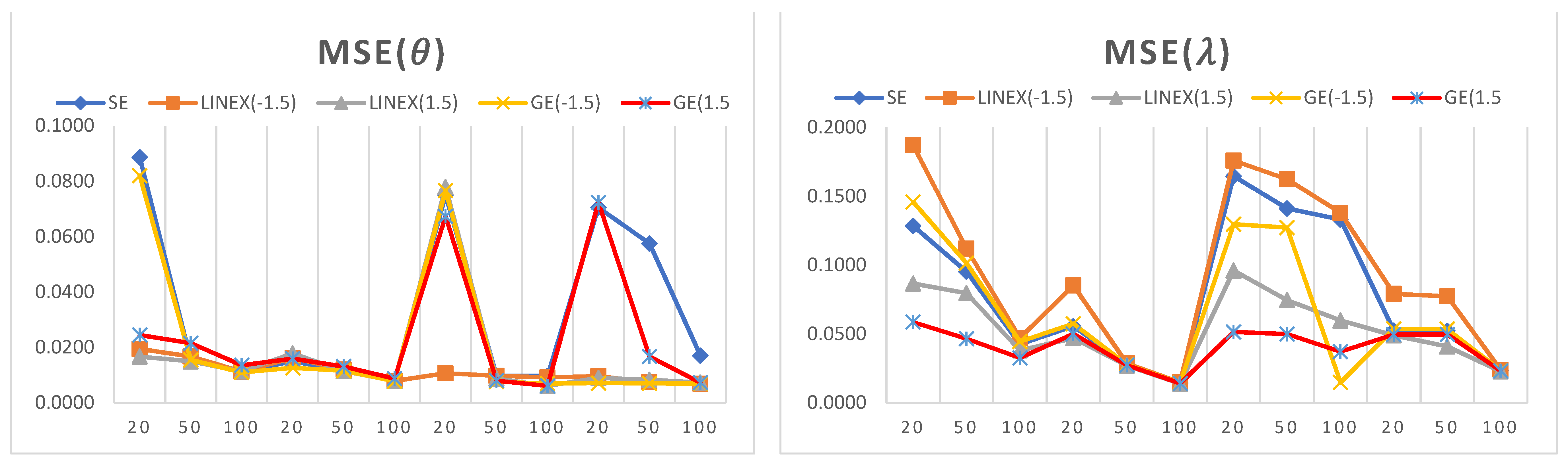
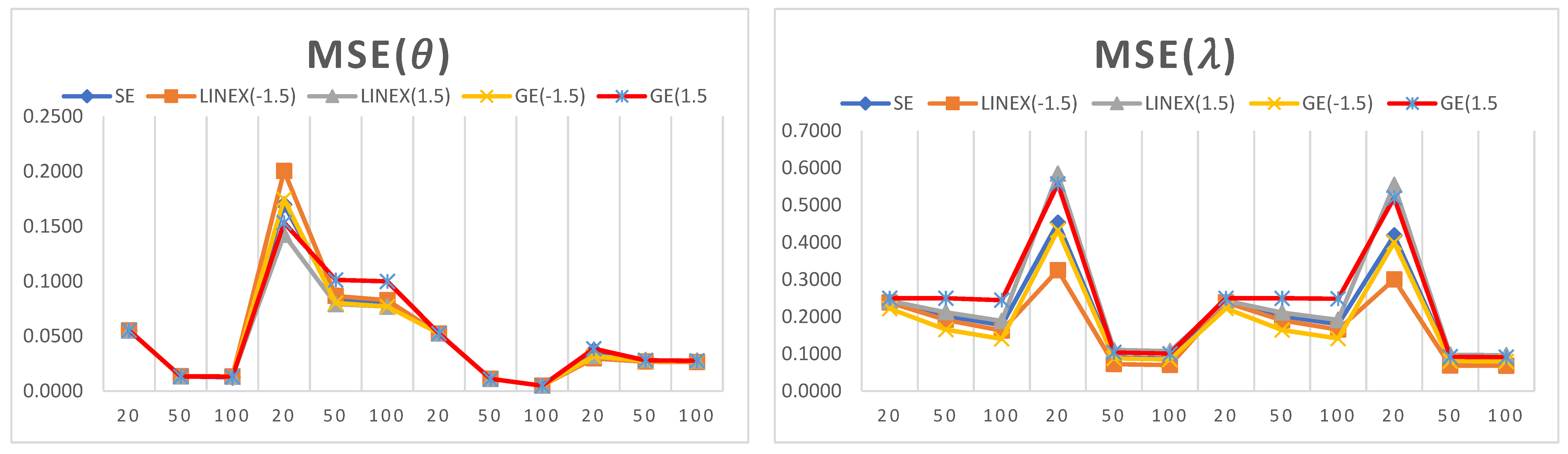
The simulation results of point and interval estimations for the three discrete versions of the GPD are reported in Table 1, Table 2 and Table 3. Figure 4, Figure 5 and Figure 6 illustrate the MSE for the simulation results in Table 1, Table 2 and Table 3. The x-axis represents sample sizes, which take values of {20,50,100}. For a fixed sample size, six different parameter values are presented. Therefore, lambda increases from 0.5 to 3 (the first six points) when theta is 0.5, and lambda increases from 0.5 to 3 (the last six points) when theta is 3.
The main simulation analysis points are as follows:
- It can be observed that the estimated values of the model parameters converge to their true values when increasing the sample size. This can be observed since the MSE and biases decrease as the sample size increases, which shows that the proposed estimators are consistent in nature.
- For a small sample size, the LINEX loss function provides the lowest values of MSE and bias when estimating , while the GE loss function provides the lowest values of MSE and bias when estimating .
- For a large sample size, the LINEX loss function provides the lowest values of MSE and bias when estimating both parameters and .
- In almost all cases, the LINEX and GE loss functions produce minimum bias and MSE values, and this is true for different sample sizes. Hence, LINEX and GE are recommended over SE in this study.
- For the credible CI, it is noted that the shortest interval length is obtained when using the LINEX loss function.
- The SE loss function has some advantages over other loss functions under some conditions; for example, when = = 3 and for a small sample size (n = 20), the bias and MSE attain their minimum values when estimating .
- For a fixed value of , the bias decreases when the shape parameter increases. Similarly, for a fixed value of , the bias decreases when increases.
- The length of the credible interval decreases when the sample size increases, and this is true for all loss functions under study.
When comparing the performance of the three DGPD analogues, we observe the following:
- For almost all small-size cases, the first discrete analogue DGPD1 has the least bias and lowest MSE for different parameter values.
- For a large sample size, it is observed that the MSE attains its minimum values when using the second analogue, DGPD2.
- The advantage of using the third analogue, DGPD3, appears when finding the credible interval for the parameter using the GE loss function, where the interval length reaches its minimum value.
5. Real Data Examples
In this section, some real data are utilized for the purpose of proving the efficiency of the discrete analogues of the GP distribution.
Some goodness-of-fit measures are used, such as the chi-square test, Kolmogorov–Smirnov (KS), Akaike information criterion (AIC), Bayesian information criterion (BIC), corrected Akaike information criterion (CAIC), and Hannan–Quinn information criterion (HQIC). As a model selection criterion, the researcher should choose the model with the minimum value from the above-mentioned measures of fit.
Data set 1: The first set of data represents a 42-day COVID-19 data set from the United States Virgin Islands, recorded between 19 April 2021 and 30 May 2021. These data comprise daily new deaths. The data are as follows: 11, 2, 3, 10, 10, 4, 12, 0, 10, 3, 5, 12, 6, 9, 13, 4, 10, 26, 0, 32, 0, 0, 13, 10, 3, 20, 5, 6, 0, 3, 18, 2, 18, 14, 24, 7, 0, 30, 16, 26, 17, 23. The data are available on the Worldometer website at [36].
Table 4 summarizes the values of goodness-of-fit measures when comparing the DGPD with nine different discrete models, including those with one, two, and three parameters. The competitive models are discrete Marshal Olkin inverted Topp–Leone (DMOITL), which is introduced in [37], Discrete Burr (DB), which is introduced in [38], discrete Weibull (DW), which is introduced in [39], discrete inverse Weibull (DIW), which is obtained in [40], negative binomial NB in [41], Poisson, discrete generalized exponential (DGE), which is introduced in [42], discrete alpha power inverse Lomax (DAPIL) in [19], and discrete Lindley (DL) in [43].
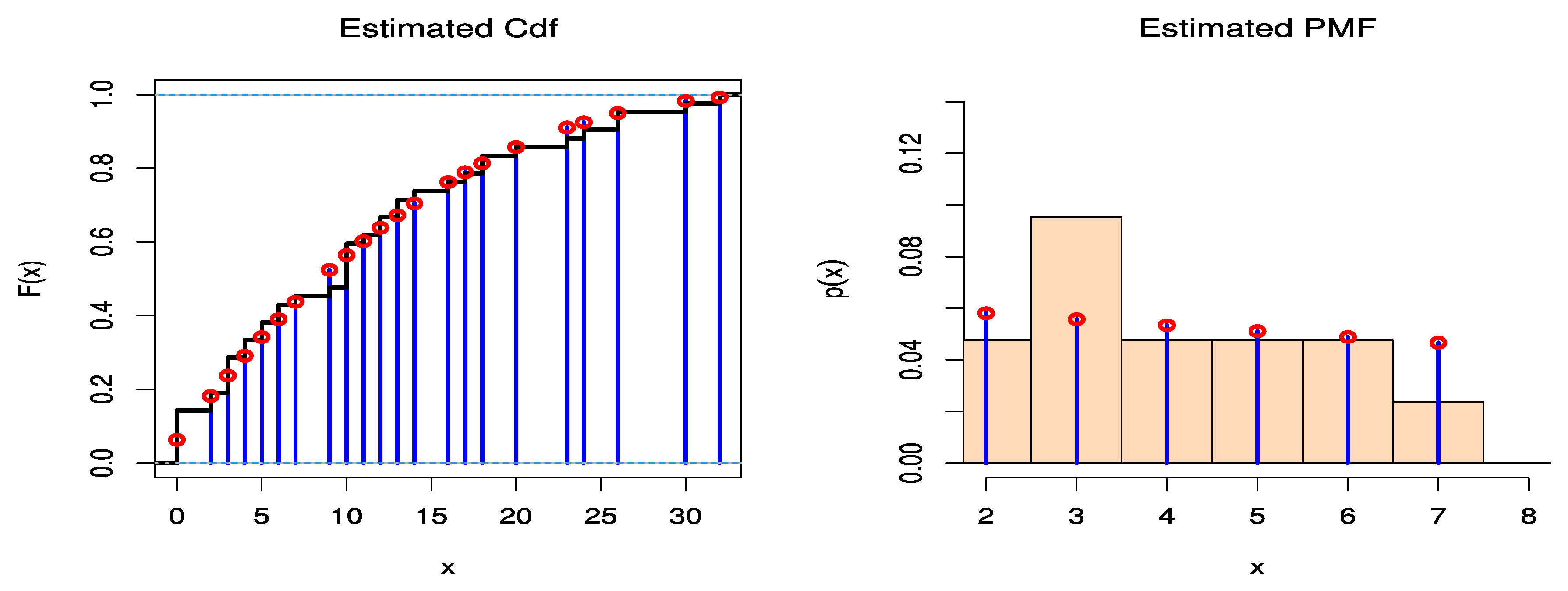
Table 4 reveals the efficiency and suitability of DGPD1 for modeling COVID-19 cases with respect to other discrete candidate models, while Figure 7 shows PMF and CDF for the fitted DGPD1 of data set 1. The distribution that has smaller values of key statistics, such as AIC, BIC, CAIC, HQIC, KS-test statistics, and Chi2-test statistics, is generally the one that fits the data the best. These statistics show that among all fitted models, the DGPD1 has the lowest KS-statistical, Chi2-statistical, AIC, BIC, CAIC, and HQIC values. The P-value of KS-test statistics and Chi2-test statistics are compared at the 5% level of significance. For data set 1, Table 5 elucidates the performance of Bayesian estimation, which is marginally better than the well-known classical maximum likelihood estimation (MLE) with respect to minimizing SE.
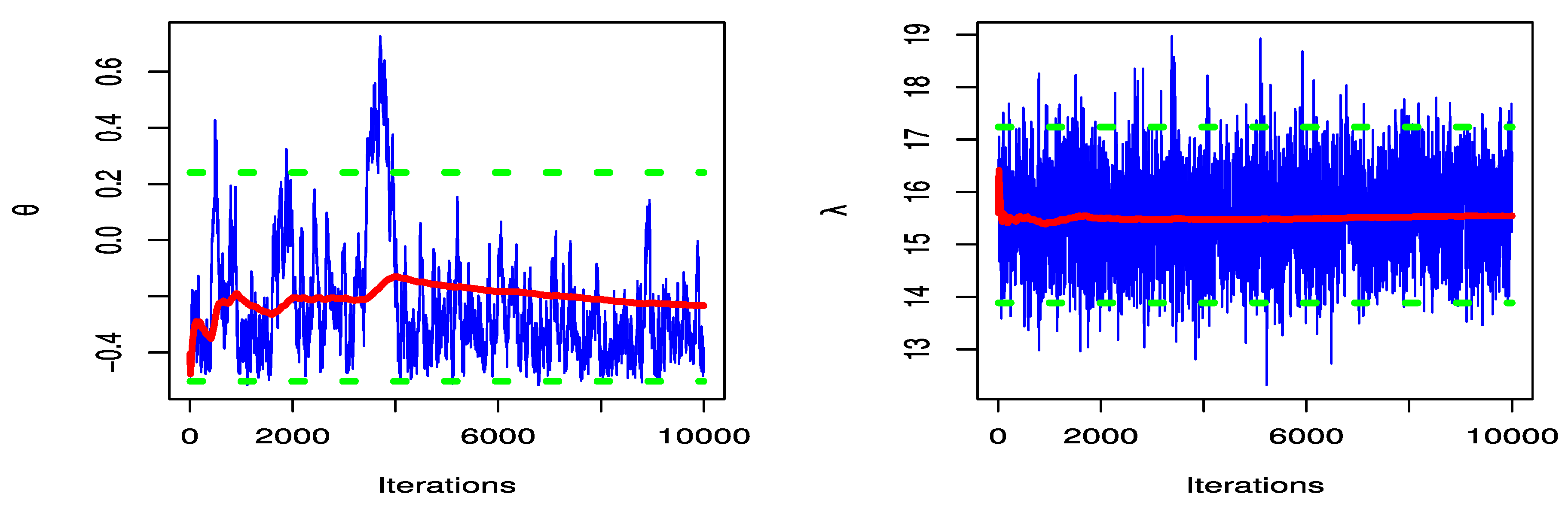
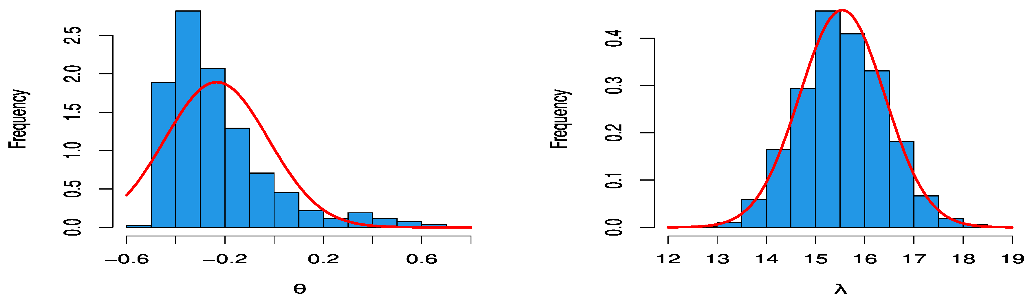
To confirm this conclusion, we should check the convergence of the MCMC results. Figure 7 shows the trace and convergence plots of MCMC for parameter estimates of DGPD1. Figure 8 depicts the MCMC convergence of and . We confirm the results of MCMC that the parameters of DGPD1 have convergence by the MH algorithm. Figure 9 shows the posterior density plots of MCMC for parameter estimates of DGPD1 for data set 1, which has a normal curve, as per the proposed distribution of the MH algorithm.
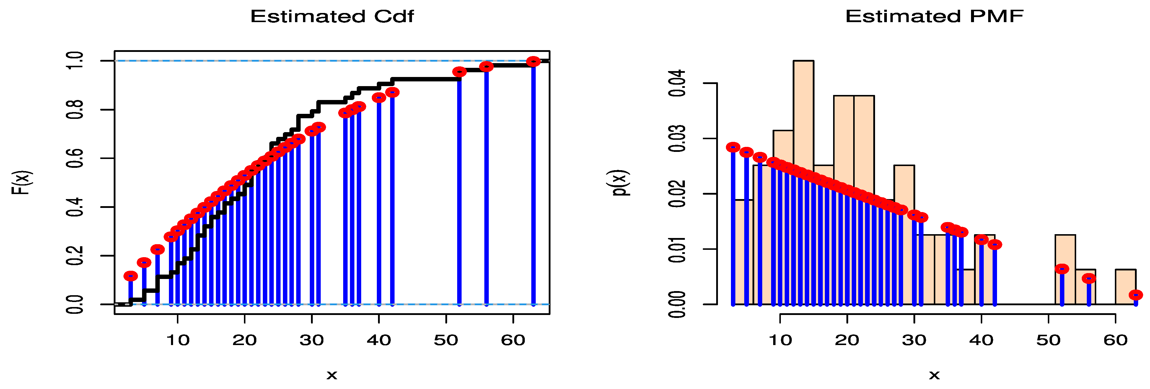
Data set 2: The second set of data represents a 53-day COVID-19 data set from Italy, recorded between 13 June 2021 and 4 August 2021. These data comprise daily new deaths. The data are as follows: 52, 26, 36, 63, 52, 37, 35, 28, 17, 21, 31, 30, 10, 56, 40, 14, 28, 42, 24, 21, 28, 22, 12, 31, 24, 14, 13, 25, 12, 7, 13, 20, 23, 9, 11, 13, 3, 7, 10, 21, 15, 17, 5, 7, 22, 24, 15, 19, 18, 16,5, 20, 27. The data are available on the Worldometer website at [36].
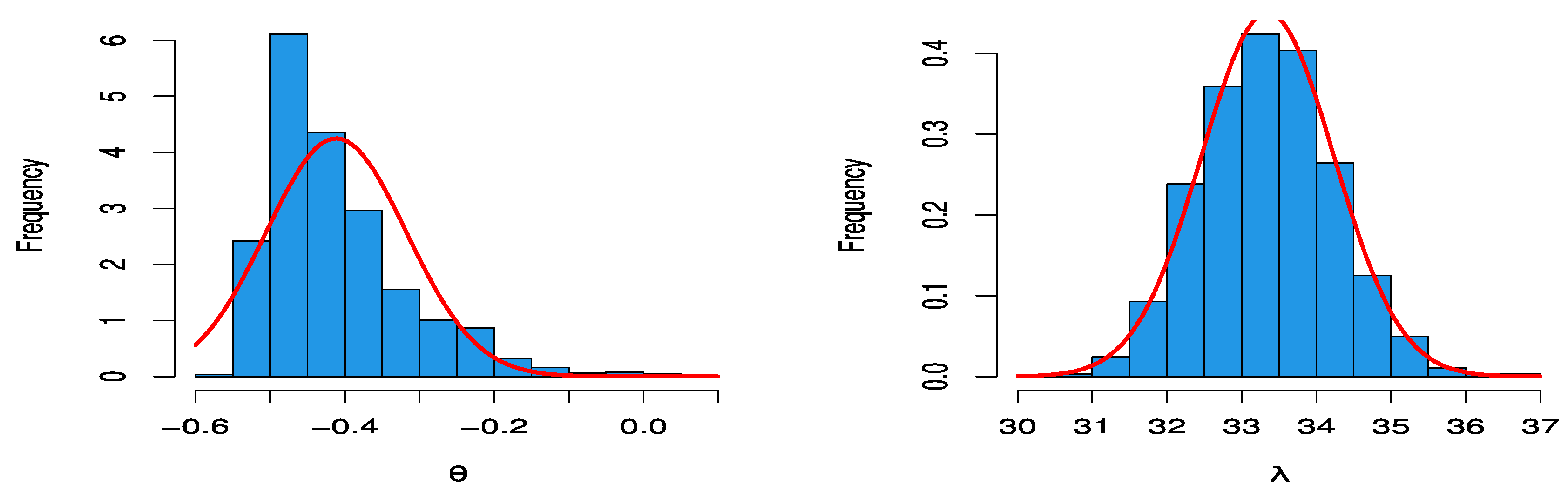
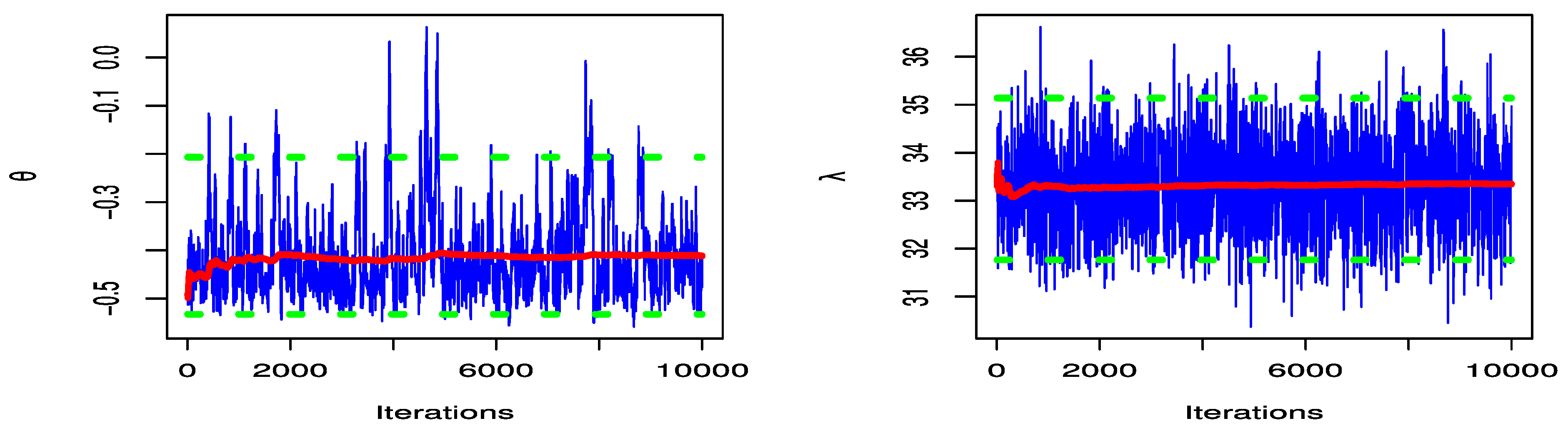
Figure 10 shows PMF and CDF for the fitted DGP of data set 2. The SE values of the parameters of DGP are shown in Table 6 to compare between MLE and Bayesian estimation methods for data set 2. From the results of SE in Table 6, we note that Bayesian estimation is a superior estimation method for data set 2 compared to MLE. Figure 11 shows that the posterior density plots of MCMC for parameter estimates of DGPD1 for data set 2 have a normal curve, as per the proposed distribution of the MH algorithm. To confirm this conclusion, we should check the convergence of the MCMC results. Figure 12 shows the trace and convergence plots of MCMC for parameter estimates of DGPD1 for data set 2. In Figure 12, we confirm that the results of MCMC for the parameters of DGPD1 have convergence by the MH algorithm.
6. Conclusions
In this study, we propose and study new discrete distributions that have a decreasing probability mass function for all choices of their parameters. The new distribution is called the discrete generalized Pareto distribution (DGPD). We used different discretization methods that introduced three discrete analogues of the DGPD. Point and interval estimations through the Bayesian method were obtained, and a simulation analysis was performed using R code to assess the efficiency of the three discrete models. Some loss functions were employed in this study, such as SE, LINEX, and GE loss functions. The tables presented in the simulation section show some good properties for each analogue. To check the validity of the DGPD, two real data examples were considered, which comprised COVID-19 death cases in two different regions. Our proposed DGPD1 was compared with other discrete candidates, and via goodness-of-fit tests, it was proved that DGPD1 fit the data very well. The tables and figures illustrate the efficiency of the new model as well. For further study, we suggest using other discretization methods and testing their performance and suitability using real-life data.
Author Contributions
Conceptualization, H.H.A. and E.M.A.; methodology, H.H.A.; software, E.M.A.; validation, H.H.A. and E.M.A.; formal analysis, H.H.A.; investigation, E.M.A.; resources, H.H.A. and E.M.A.; data curation, E.M.A.; writing—original draft preparation, H.H.A.; writing—review and editing, H.H.A. and E.M.A.; visualization, E.M.A.; supervision, H.H.A.; project administration, H.H.A.; funding acquisition, H.H.A. All authors have read and agreed to the published version of the manuscript.
Funding
This work was supported through the Annual Funding track by the Deanship of Scientific Research, Vice Presidency for Graduate Studies and Scientific Research, King Faisal University, Saudi Arabia [Project No. AN000537].
Institutional Review Board Statement
Not applicable.
Informed Consent Statement
Not applicable.
Data Availability Statement
The data is available in the text of this article.
Conflicts of Interest
The authors declare no conflict of interest.
References
- Xekalaki, E. Hazard function and life distributions in discrete time. Commun. Stat. Theory Methods 1983, 12, 2503–2509. [Google Scholar] [CrossRef]
- Hitha, N.; Nair, N.U. Characterization of some discrete models by properties of residual life function. Calcutta Stat. Assoc. Bull. 1989, 38, 219–223. [Google Scholar] [CrossRef]
- Roy, D.; Gupta, R.P. Classifications of discrete lives. Microelectron. Reliab. 1992, 32, 459–1473. [Google Scholar] [CrossRef]
- Roy, D.; Gupta, R.P. Stochastic modeling through reliability measures in the discrete case. Stat. Probab. Lett. 1999, 43, 197–206. [Google Scholar] [CrossRef]
- Roy, D. On classifications of multivariate life distributions in the discrete set-up. Microelectron. Reliab. 1997, 37, 361–366. [Google Scholar] [CrossRef]
- Roy, D. The discrete normal distribution. Commun. Stat. Theory Methods 2003, 32, 1871–1883. [Google Scholar] [CrossRef]
- Roy, D. Discrete Rayleigh distribution. IEEE. Trans. Reliab. 2004, 53, 255–260. [Google Scholar] [CrossRef]
- Roy, D.; Ghosh, T. A New Discretization Approach with Application in Reliability Estimation. IEEE Trans. Reliab. 2009, 58, 456–461. [Google Scholar] [CrossRef]
- Bracquemond, C.; Gaudoin, O. A survey on discrete life time distributions. Int. J. Reliab. Qual. Saf. Eng. 2003, 10, 69–98. [Google Scholar] [CrossRef]
- Lai, C.D. Issues concerning constructions of discrete lifetime models. Qual. Technol. Quant. Manag. 2013, 10, 251–262. [Google Scholar] [CrossRef]
- Chakraborty, S. Generating discrete analogues of continuous probability distributions—A survey of methods and constructions. J. Stat. Distrib. Appl. 2015, 2, 6. [Google Scholar] [CrossRef] [Green Version]
- Liu, H.; Hussain, F.; Tan, C.L.; Dash, M. Discretization: An Enabling Technique. Data Min. Knowl. Discov. 2002, 6, 393–423. [Google Scholar] [CrossRef]
- Arnastauskaitė, J.; Ruzgas, T.; Bražėnas, M. An Exhaustive Power Comparison of Normality Tests. Mathematics 2021, 9, 788. [Google Scholar] [CrossRef]
- Korkmaz, S.; Goksuluk, D.; Zararsiz, G. MVN: An R Package for Assessing Multivariate Normality. R J. 2014, 6, 151–162. [Google Scholar] [CrossRef] [Green Version]
- Al-Huniti, A.A.; AL-Dayian, G.R. Discrete Burr type III distribution. Am. J. Math. Stat. 2012, 2, 145–152. [Google Scholar] [CrossRef]
- Bebbington, M.; Lai, C.D.; Wellington, M.; Zitikis, R. The discrete additive Weibull distribution: A bathtub-shaped hazard for discontinuous failure data. Reliab. Eng. Syst. Saf. 2012, 106, 37–44. [Google Scholar] [CrossRef]
- Sarhan, A.M. A two-parameter discrete distribution with a bathtub hazard shape. Commun. Stat. Appl. Methods 2017, 24, 15–27. [Google Scholar] [CrossRef] [Green Version]
- Yari, G.; Tondpour, Z. Discrete Burr XII-Gamma Distributions: Properties and Parameter Estimations. Iran. J. Sci. Technol. Trans. A Sci. 2018, 42, 2237–2249. [Google Scholar] [CrossRef]
- Almetwally, E.M.; Ibrahim, G.M. Discrete Alpha Power Inverse Lomax Distribution with Application of COVID-19 Data. Int. J. Appl. Math. 2020, 9, 11–22. [Google Scholar]
- Eliwa, M.S.; Altun, E.; El-Dawoody, M.; El-Morshedy, M. A new three-parameter discrete distribution with associated INAR (1) process and applications. IEEE Access 2020, 8, 91150–91162. [Google Scholar] [CrossRef]
- Almetwally, E.M.; Almongy, H.M.; Saleh, H.A. Managing risk of spreading “COVID-19” in Egypt: Modelling using a discrete Marshall-Olkin generalized exponential distribution. Int. J. Probab. Stat. 2020, 9, 33–41. [Google Scholar]
- Al-Babtain, A.A.; Ahmed, A.H.N.; Afify, A.Z. A New Discrete Analog of the Continuous Lindley Distribution, with Reliability Applications. Entropy 2020, 22, 603. [Google Scholar] [CrossRef] [PubMed]
- Eldeeb, A.S.; Ahsan-Ul-Haq, M.; Babar, A. A Discrete Analog of Inverted Topp-Leone Distribution: Properties, Estimation and Applications. Int. J. Anal. Appl. 2021, 19, 695–708. [Google Scholar]
- Elbatal, I.; Alotaibi, N.; Almetwally, E.M.; Alyami, S.A.; Elgarhy, M. On Odd Perks-G Class of Distributions: Properties, Regression Model, Discretization, Bayesian and Non-Bayesian Estimation, and Applications. Symmetry 2022, 14, 883. [Google Scholar] [CrossRef]
- Nagy, M.; Almetwally, E.M.; Gemeay, A.M.; Mohammed, H.S.; Jawa, T.M.; Sayed-Ahmed, N.; Muse, A.H. The new novel discrete distribution with application on covid-19 mortality numbers in Kingdom of Saudi Arabia and Latvia. Complexity 2021, 2021, 7192833. [Google Scholar] [CrossRef]
- Gillariose, J.; Balogun, O.S.; Almetwally, E.M.; Sherwani, R.A.K.; Jamal, F.; Joseph, J. On the Discrete Weibull Marshall–Olkin Family of Distributions: Properties, Characterizations, and Applications. Axioms 2021, 10, 287. [Google Scholar] [CrossRef]
- Martín, J.; Parra, M.I.; Pizarro, M.M.; Sanjuán, E.L. Baseline Methods for the Parameter Estimation of the Generalized Pareto Distribution. Entropy 2022, 24, 178. [Google Scholar] [CrossRef]
- Huang, C.; Zhao, X.; Cheng, W.; Ji, Q.; Duan, Q.; Han, Y. Statistical Inference of Dynamic Conditional Generalized Pareto Distribution with Weather and Air Quality Factors. Mathematics 2022, 10, 1433. [Google Scholar] [CrossRef]
- Shui, P.-L.; Zou, P.-J.; Feng, T. Outlier-robust truncated maximum likelihood parameter estimators of generalized Pareto distributions. Digit. Signal Process. 2022, 127, 103527. [Google Scholar] [CrossRef]
- He, Y.; Peng, L.; Zhang, D.; Zhao, Z. Risk Analysis via Generalized Pareto Distributions. J. Bus. Econ. Stat. 2021, 40, 852–867. [Google Scholar] [CrossRef]
- Arnold, B.C.; Press, S.J. Compatible Conditional Distributions. J. Am. Stat. Assoc. 1989, 84, 152. [Google Scholar] [CrossRef]
- Karandikar, R.L. On the Markov Chain Monte Carlo (MCMC) method. Sadhana 2006, 31, 81–104. [Google Scholar] [CrossRef] [Green Version]
- Wang, Y.; Zhang, J.; Cai, C.; Lu, W.; Tang, Y. Semiparametric estimation for proportional hazards mixture cure model allowing non-curable competing risk. J. Stat. Plan. Inference 2020, 211, 171–189. [Google Scholar] [CrossRef]
- Xu, A.; Zhou, S.; Tang, Y. A unified model for system reliability evaluation under dynamic operating conditions. IEEE Trans. Reliab. 2021, 70, 65–72. [Google Scholar] [CrossRef]
- Luo, C.; Shen, L.; Xu, A. Modelling and estimation of system reliability under dynamic operating environments and lifetime ordering constraints. Reliab. Eng. Syst. Saf. 2022, 218, 108136. [Google Scholar] [CrossRef]
- Worldometers. Available online: https://www.worldometers.info/coronavirus. (accessed on 1 June 2021).
- Almetwally, E.M.; Abdo, D.A.; Hafez, E.H.; Jawa, T.M.; Sayed-Ahmed, N.; Almongy, H.M. The new discrete distribution with application to COVID-19 Data. Results Phys. 2021, 32, 104987. [Google Scholar] [CrossRef]
- Krishna, H.; Pundir, P.S. Discrete Burr and discrete Pareto distributions. Stat. Methodol. 2009, 6, 177–188. [Google Scholar] [CrossRef]
- Khan, M.A.; Khalique, A.; Abouammoh, A.M. On estimating parameters in a discrete Weibull distribution. IEEE Trans. Reliab. 1989, 38, 348–350. [Google Scholar] [CrossRef]
- Jazi, M.A.; Lai, C.-D.; Alamatsaz, M.H. A discrete inverse Weibull distribution and estimation of its parameters. Stat. Methodol. 2010, 7, 121–132. [Google Scholar] [CrossRef]
- Fisher, P. Negative Binomial Distribution. Ann. Eugen. 1941, 11, 182–787. [Google Scholar] [CrossRef]
- Nekoukhou, V.; Alamatsaz, M.H.; Bidram, H. Discrete generalized exponential distribution of a second type. Statistics 2013, 47, 876–887. [Google Scholar] [CrossRef]
- Gómez-Déniz, E.; Calderín-Ojeda, E. The discrete Lindley distribution: Properties and applications. J. Stat. Comput. Simul. 2011, 81, 1405–1416. [Google Scholar] [CrossRef]
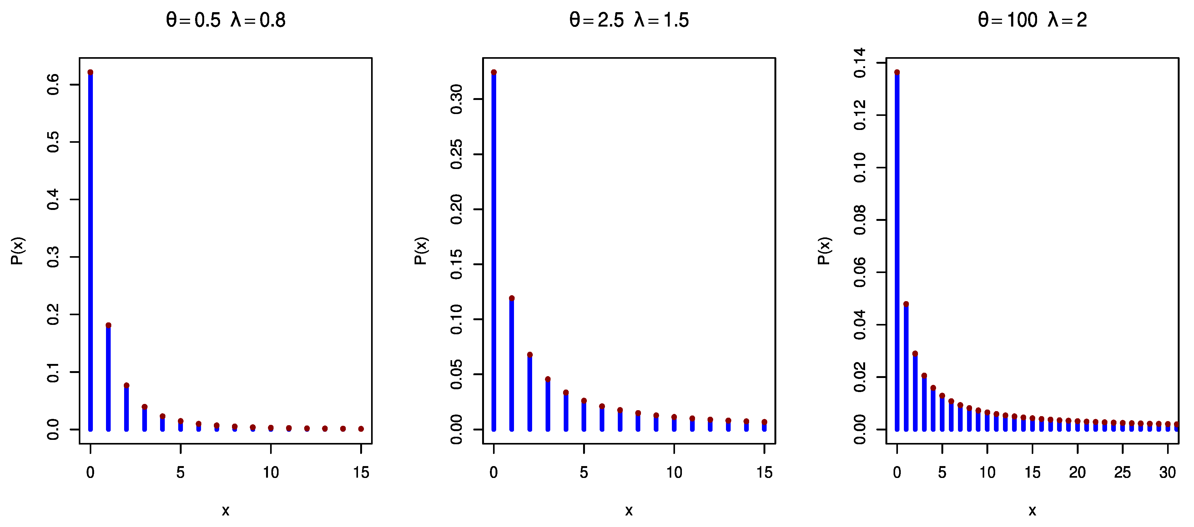
Figure 1.
Plots of pmf of the DGPD1 distribution with different values of the parameters .

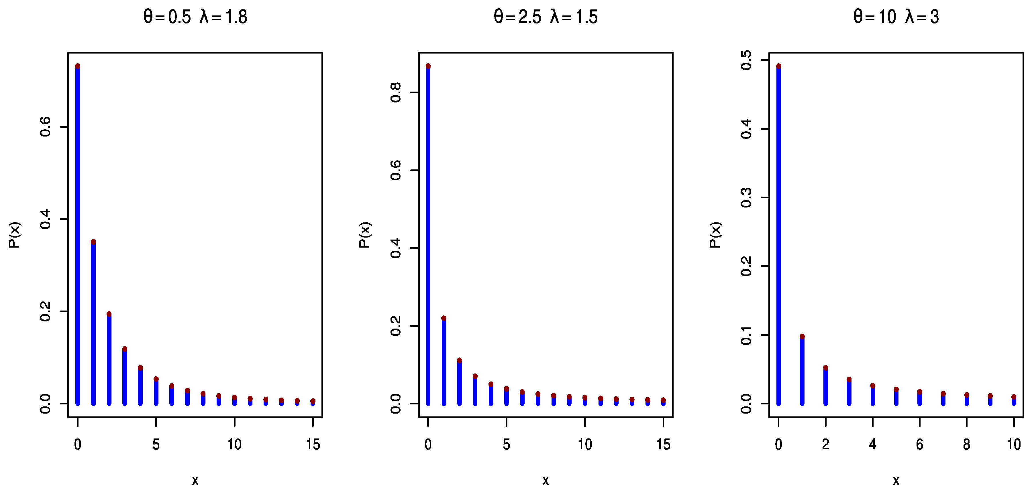
Figure 2.
Plots of pmf of the DGPD2 distribution with different values of the parameters .

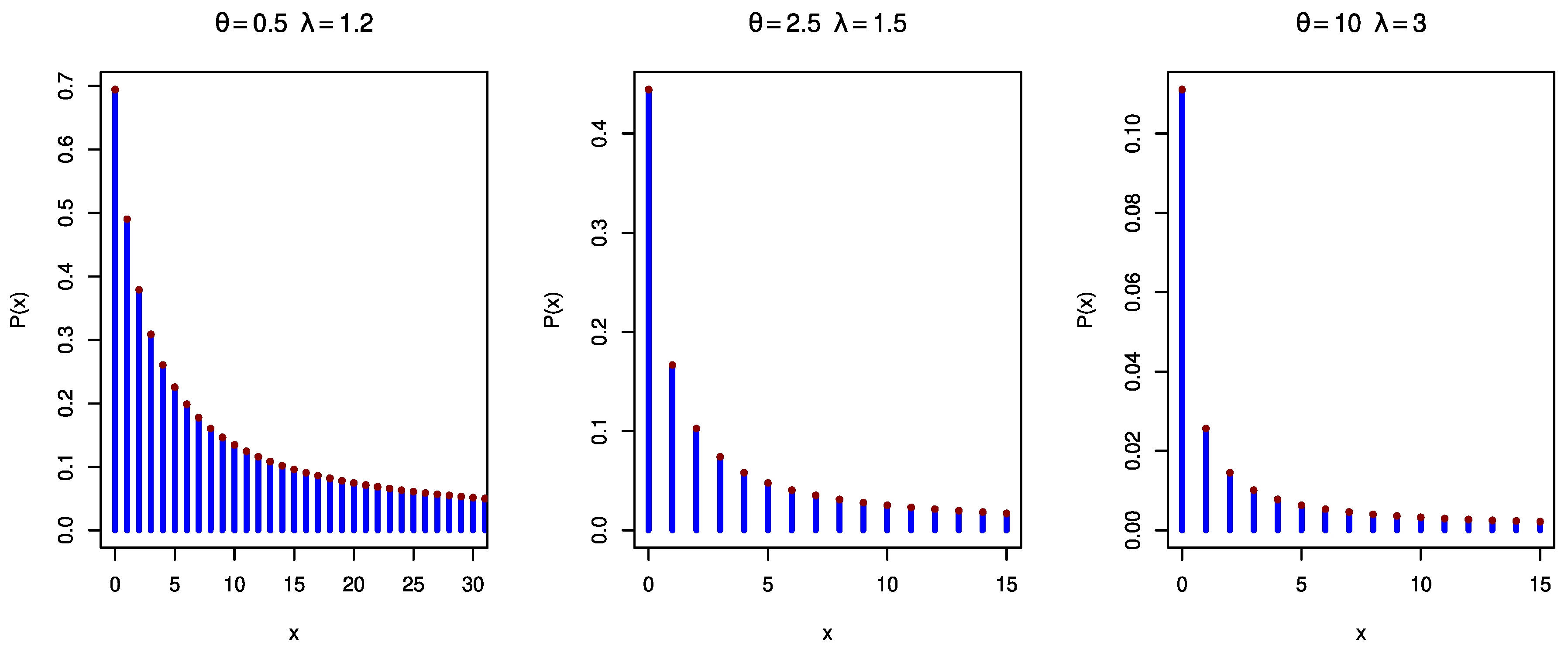
Figure 3.
Plots of the pmf of the DGPD3 distribution with different values of the parameters .

Figure 4.
MSE of Bayesian inference for DGPD1.

Figure 5.
MSE of Bayesian inference for DGPD2.

Figure 6.
MSE of Bayesian inference for DGPD3.

Figure 7.
Plots of estimated pmf and CDF of DGPD1 for data set I.

Figure 8.
Trace and convergence plots of MCMC for parameter estimates of DGPD1 for data set I.

Figure 9.
Posterior density plots of MCMC for parameter estimates of DGPD1 for data set I.

Figure 10.
Plots of estimated pmf and CDF of DGPD1 for data set 2.

Figure 11.
Posterior density plots of MCMC for parameter estimates of DGPD1 for data set 2.

Figure 12.
Trace and convergence plots of MCMC for parameter estimates of DGPD1 for data set 2.


Table 1.
Bayesian inference for DGPD1 (bias, MSE, and length of CI) for different values of parameters.
Table 1.
Bayesian inference for DGPD1 (bias, MSE, and length of CI) for different values of parameters.
| SE | LINEX (−1.5) | LINEX (1.5) | GE (−1.5) | GE (1.5) | ||||||||||||||
|---|---|---|---|---|---|---|---|---|---|---|---|---|---|---|---|---|---|---|
| n | Bias | MSE | L.CCI | Bias | MSE | L.CCI | Bias | MSE | L.CCI | Bias | MSE | L.CCI | Bias | MSE | L.CCI | |||
| 0.5 | 0.5 | 20 | 0.0247 | 0.0887 | 0.5335 | 0.0601 | 0.0194 | 0.4371 | −0.0066 | 0.0167 | 0.4630 | 0.0450 | 0.0820 | 0.6443 | −0.0870 | 0.0245 | 0.4930 | |
| 0.2946 | 0.1284 | 0.7412 | 0.3597 | 0.1870 | 0.8541 | 0.2368 | 0.0866 | 0.6692 | 0.3190 | 0.1458 | 0.7567 | 0.1631 | 0.0586 | 0.6918 | ||||
| 50 | −0.0130 | 0.0155 | 0.4394 | 0.0034 | 0.0167 | 0.4526 | −0.0289 | 0.0150 | 0.4294 | −0.0020 | 0.0155 | 0.4396 | −0.0750 | 0.0215 | 0.4590 | |||
| 0.2666 | 0.0952 | 0.6031 | 0.2901 | 0.1120 | 0.6405 | 0.2429 | 0.0796 | 0.5616 | 0.2764 | 0.1014 | 0.6067 | 0.2132 | 0.0465 | 0.5528 | ||||
| 100 | −0.0084 | 0.0112 | 0.4062 | −0.0025 | 0.0112 | 0.4070 | −0.0144 | 0.0113 | 0.4062 | −0.0041 | 0.0110 | 0.4023 | −0.0316 | 0.0136 | 0.4360 | |||
| 0.1827 | 0.0424 | 0.3745 | 0.1923 | 0.0470 | 0.3914 | 0.1729 | 0.0381 | 0.3569 | 0.1872 | 0.0444 | 0.3781 | 0.1586 | 0.0326 | 0.3407 | ||||
| 3 | 20 | 0.0353 | 0.0150 | 0.4610 | 0.0680 | 0.0162 | 0.4588 | 0.0064 | 0.0178 | 0.4533 | 0.0537 | 0.0126 | 0.4755 | −0.0642 | 0.0159 | 0.4910 | ||
| 0.0704 | 0.0555 | 0.8743 | 0.1615 | 0.0852 | 0.9396 | −0.0176 | 0.0469 | 0.8464 | 0.0803 | 0.0574 | 0.8773 | 0.0206 | 0.0500 | 0.8675 | ||||
| 50 | 0.0009 | 0.0116 | 0.4267 | 0.0080 | 0.0120 | 0.4324 | −0.0062 | 0.0114 | 0.4220 | 0.0057 | 0.0116 | 0.4274 | −0.0248 | 0.0131 | 0.4528 | |||
| 0.0192 | 0.0276 | 0.6226 | 0.0301 | 0.0287 | 0.6274 | 0.0084 | 0.0269 | 0.6189 | 0.0204 | 0.0277 | 0.6217 | 0.0132 | 0.0274 | 0.6259 | ||||
| 100 | −0.0080 | 0.0079 | 0.3509 | −0.0042 | 0.0079 | 0.3511 | −0.0117 | 0.0079 | 0.3508 | −0.0054 | 0.0078 | 0.3480 | −0.0214 | 0.0087 | 0.3554 | |||
| 0.0230 | 0.0143 | 0.4554 | 0.0285 | 0.0148 | 0.4601 | 0.0175 | 0.0139 | 0.4513 | 0.0236 | 0.0143 | 0.4552 | 0.0200 | 0.0141 | 0.4526 | ||||
| 3 | 0.5 | 20 | 0.0121 | 0.0751 | 0.3389 | 0.0512 | 0.0107 | 0.3506 | −0.0595 | 0.0779 | 0.3306 | 0.0164 | 0.0766 | 0.3387 | −0.0935 | 0.0674 | 0.3351 | |
| 0.2173 | 0.1645 | 0.8449 | 0.4302 | 0.1759 | 1.0064 | 0.2412 | 0.0961 | 0.7222 | 0.2527 | 0.1297 | 0.8780 | 0.2331 | 0.0514 | 0.7289 | ||||
| 50 | −0.0037 | 0.0098 | 0.3079 | 0.0348 | 0.0098 | 0.3335 | −0.0405 | 0.0087 | 0.2944 | 0.0005 | 0.0076 | 0.3612 | −0.0245 | 0.0080 | 0.2998 | |||
| 0.2719 | 0.1411 | 0.5948 | 0.3410 | 0.1623 | 0.6569 | 0.2115 | 0.0745 | 0.5119 | 0.2499 | 0.1272 | 0.6932 | 0.1251 | 0.0499 | 0.5576 | ||||
| 100 | −0.0321 | 0.0097 | 0.3052 | 0.0018 | 0.0092 | 0.3060 | −0.0655 | 0.0061 | 0.2343 | −0.0284 | 0.0069 | 0.3509 | −0.0151 | 0.0061 | 0.2534 | |||
| 0.1317 | 0.1330 | 0.5668 | 0.3723 | 0.1380 | 0.6074 | 0.2068 | 0.0598 | 0.5096 | 0.2338 | 0.0148 | 0.6809 | 0.1021 | 0.0371 | 0.4620 | ||||
| 3 | 20 | 0.0039 | 0.0705 | 0.3629 | 0.0430 | 0.0096 | 0.4776 | −0.0339 | 0.0090 | 0.3625 | 0.0082 | 0.0071 | 0.3986 | −0.0175 | 0.0724 | 0.4327 | ||
| 0.0440 | 0.0524 | 0.8789 | 0.1402 | 0.0791 | 0.9525 | −0.0487 | 0.0489 | 0.8914 | 0.0545 | 0.0538 | 0.8868 | −0.0091 | 0.0496 | 0.8982 | ||||
| 50 | 0.0038 | 0.0575 | 0.3339 | 0.0421 | 0.0075 | 0.3526 | −0.0333 | 0.0083 | 0.3348 | 0.0080 | 0.0070 | 0.3368 | −0.0172 | 0.0167 | 0.3383 | |||
| 0.0443 | 0.0522 | 0.8095 | 0.1370 | 0.0773 | 0.8957 | −0.0451 | 0.0409 | 0.8679 | 0.0544 | 0.0535 | 0.7960 | −0.0069 | 0.0497 | 0.8517 | ||||
| 100 | −0.0152 | 0.0170 | 0.3049 | −0.0080 | 0.0069 | 0.3489 | −0.0224 | 0.0073 | 0.4917 | −0.0144 | 0.0069 | 0.3049 | −0.0192 | 0.0072 | 0.2491 | |||
| 0.0112 | 0.0233 | 0.5707 | 0.0197 | 0.0240 | 0.5772 | 0.0028 | 0.0228 | 0.5787 | 0.0122 | 0.0234 | 0.5702 | 0.0065 | 0.0231 | 0.5744 | ||||
Table 2.
Bayesian inference for DGPD2 (bias, MSE, and length of CI) for different values of parameters.
Table 2.
Bayesian inference for DGPD2 (bias, MSE, and length of CI) for different values of parameters.
| SE | LINEX (−1.5) | LINEX (1.5) | GE (−1.5) | GE (1.5) | ||||||||||||||
|---|---|---|---|---|---|---|---|---|---|---|---|---|---|---|---|---|---|---|
| n | Bias | MSE | L.CCI | Bias | MSE | L.CCI | Bias | MSE | L.CCI | Bias | MSE | L.CCI | Bias | MSE | L.CCI | |||
| 0.5 | 0.5 | 20 | −0.1145 | 0.0668 | 0.7749 | −0.1110 | 0.0652 | 0.7740 | −0.1177 | 0.0681 | 0.7734 | −0.1086 | 0.0630 | 0.7578 | −0.1349 | 0.0793 | 0.7870 | |
| −0.4889 | 0.2491 | 0.0185 | −0.4856 | 0.2459 | 0.0247 | −0.4911 | 0.2412 | 0.0142 | −0.4684 | 0.2296 | 0.0421 | −0.4993 | 0.2493 | 0.0039 | ||||
| 50 | −0.0972 | 0.0525 | 0.7273 | −0.0951 | 0.0518 | 0.7252 | −0.0991 | 0.0531 | 0.7284 | −0.0945 | 0.0511 | 0.7180 | −0.1075 | 0.0574 | 0.7516 | |||
| −0.4901 | 0.2402 | 0.0177 | −0.4878 | 0.2380 | 0.0204 | −0.4916 | 0.2417 | 0.0157 | −0.4732 | 0.2240 | 0.0291 | −0.4980 | 0.2480 | 0.0092 | ||||
| 100 | −0.0522 | 0.0186 | 0.4950 | −0.0515 | 0.0184 | 0.4941 | −0.0529 | 0.0187 | 0.4963 | −0.0516 | 0.0184 | 0.4927 | −0.0550 | 0.0192 | 0.4994 | |||
| −0.4747 | 0.2254 | 0.0255 | −0.4696 | 0.2206 | 0.0293 | −0.4782 | 0.2288 | 0.0243 | −0.4505 | 0.2031 | 0.0335 | −0.4919 | 0.2420 | 0.0193 | ||||
| 3 | 20 | 0.1424 | 0.0378 | 0.4501 | 0.1906 | 0.0604 | 0.5041 | 0.1000 | 0.0234 | 0.4023 | 0.1647 | 0.0459 | 0.4579 | 0.0206 | 0.0143 | 0.4190 | ||
| −0.0366 | 0.0591 | 0.8932 | 0.0534 | 0.0699 | 0.9843 | −0.1246 | 0.0681 | 0.8693 | −0.0265 | 0.0588 | 0.9016 | −0.0881 | 0.0641 | 0.8811 | ||||
| 50 | 0.0248 | 0.0145 | 0.4295 | 0.0328 | 0.0154 | 0.4373 | 0.0167 | 0.0138 | 0.4241 | 0.0300 | 0.0147 | 0.4286 | −0.0031 | 0.0137 | 0.4048 | |||
| −0.0371 | 0.0312 | 0.6886 | −0.0256 | 0.0300 | 0.6766 | −0.0487 | 0.0327 | 0.6941 | −0.0358 | 0.0310 | 0.6877 | −0.0437 | 0.0323 | 0.6971 | ||||
| 100 | 0.0068 | 0.0077 | 0.3405 | 0.0104 | 0.0078 | 0.3384 | 0.0032 | 0.0075 | 0.3367 | 0.0092 | 0.0077 | 0.3346 | −0.0056 | 0.0079 | 0.3475 | |||
| −0.0257 | 0.0113 | 0.4118 | −0.0213 | 0.0109 | 0.4001 | −0.0302 | 0.0117 | 0.4212 | −0.0252 | 0.0113 | 0.4104 | −0.0283 | 0.0116 | 0.4019 | ||||
| 3 | 0.5 | 20 | 0.0315 | 0.0547 | 0.9001 | 0.0348 | 0.0549 | 0.9038 | 0.0282 | 0.0543 | 0.8926 | 0.0318 | 0.0547 | 0.9004 | 0.0297 | 0.0546 | 0.8976 | |
| −0.4798 | 0.2309 | 0.0569 | −0.4715 | 0.2240 | 0.0845 | −0.4850 | 0.2355 | 0.0409 | −0.4503 | 0.2046 | 0.1119 | −0.4998 | 0.2498 | 0.0006 | ||||
| 50 | 0.0211 | 0.0169 | 0.4877 | 0.0234 | 0.0171 | 0.4883 | 0.0187 | 0.0166 | 0.4842 | 0.0214 | 0.0169 | 0.4879 | 0.0198 | 0.0168 | 0.4854 | |||
| −0.3902 | 0.1568 | 0.2287 | −0.3676 | 0.1406 | 0.2581 | −0.4090 | 0.1710 | 0.1935 | −0.3388 | 0.1195 | 0.2469 | −0.4981 | 0.2490 | 0.0003 | ||||
| 100 | 0.0183 | 0.0085 | 0.3602 | 0.0199 | 0.0086 | 0.3628 | 0.0166 | 0.0083 | 0.3570 | 0.0184 | 0.0085 | 0.3605 | 0.0173 | 0.0084 | 0.3587 | |||
| −0.3494 | 0.1252 | 0.1901 | −0.3246 | 0.1087 | 0.2058 | −0.3715 | 0.1407 | 0.1709 | −0.3002 | 0.0929 | 0.1893 | −0.4992 | 0.2049 | 0.0002 | ||||
| 3 | 20 | 0.0932 | 0.0255 | 0.6319 | 0.1333 | 0.0251 | 0.3280 | 0.0544 | 0.0195 | 0.5306 | 0.0975 | 0.0263 | 0.5319 | 0.0719 | 0.0219 | 0.5632 | ||
| 0.0225 | 0.0618 | 0.9381 | 0.1175 | 0.0857 | 1.0463 | −0.0703 | 0.0608 | 0.8915 | 0.0330 | 0.0629 | 0.9506 | −0.0309 | 0.0606 | 0.8925 | ||||
| 50 | 0.0546 | 0.0203 | 0.5208 | 0.0640 | 0.0219 | 0.5218 | 0.0453 | 0.0189 | 0.5090 | 0.0556 | 0.0204 | 0.5209 | 0.0495 | 0.0196 | 0.5177 | |||
| −0.0173 | 0.0281 | 0.6513 | −0.0059 | 0.0272 | 0.6505 | −0.0287 | 0.0293 | 0.6510 | −0.0160 | 0.0279 | 0.6504 | −0.0238 | 0.0290 | 0.6459 | ||||
| 100 | 0.0451 | 0.0115 | 0.3816 | 0.0495 | 0.0123 | 0.3872 | 0.0406 | 0.0107 | 0.3728 | 0.0455 | 0.0116 | 0.3835 | 0.0426 | 0.0111 | 0.3791 | |||
| −0.0042 | 0.0115 | 0.4137 | 0.0000 | 0.0115 | 0.4164 | −0.0083 | 0.0117 | 0.4146 | −0.0037 | 0.0115 | 0.4138 | −0.0065 | 0.0116 | 0.4162 | ||||
Table 3.
Bayesian inference for DGPD3 (bias, MSE, and length of CI) for different values of parameters.
Table 3.
Bayesian inference for DGPD3 (bias, MSE, and length of CI) for different values of parameters.
| SE | LINEX (−1.5) | LINEX (1.5) | GE (−1.5) | GE (1.5) | ||||||||||||||
|---|---|---|---|---|---|---|---|---|---|---|---|---|---|---|---|---|---|---|
| n | Bias | MSE | L.CCI | Bias | MSE | L.CCI | Bias | MSE | L.CCI | Bias | MSE | L.CCI | Bias | MSE | L.CCI | |||
| 0.5 | 0.5 | 20 | 0.0231 | 0.0552 | 0.9405 | 0.0248 | 0.0552 | 0.9396 | 0.0214 | 0.0550 | 0.9399 | 0.0236 | 0.0552 | 0.9397 | 0.0208 | 0.0552 | 0.9422 | |
| −0.4908 | 0.2409 | 0.0134 | −0.4879 | 0.2381 | 0.0189 | −0.4927 | 0.2428 | 0.0097 | −0.4710 | 0.2219 | 0.0349 | −0.4998 | 0.2498 | 0.0005 | ||||
| 50 | 0.0067 | 0.0134 | 0.4749 | 0.0075 | 0.0135 | 0.4757 | 0.0058 | 0.0133 | 0.4719 | 0.0069 | 0.0134 | 0.4750 | 0.0055 | 0.0133 | 0.4718 | |||
| −0.4505 | 0.2032 | 0.0495 | −0.4374 | 0.1916 | 0.0645 | −0.4603 | 0.2120 | 0.0397 | −0.4064 | 0.1655 | 0.0713 | −0.4999 | 0.2499 | 0.0002 | ||||
| 100 | 0.0291 | 0.0124 | 0.4307 | 0.0303 | 0.0134 | 0.4333 | 0.0028 | 0.0131 | 0.4255 | 0.0295 | 0.0130 | 0.4312 | 0.0274 | 0.0131 | 0.4246 | |||
| −0.4204 | 0.1771 | 0.0642 | −0.4030 | 0.1628 | 0.0796 | −0.4342 | 0.1887 | 0.0521 | −0.3742 | 0.1405 | 0.0841 | −0.4946 | 0.2446 | 0.0097 | ||||
| 3 | 20 | 0.0783 | 0.1698 | 1.3450 | 0.1181 | 0.2003 | 1.3980 | 0.0418 | 0.1425 | 1.2318 | 0.0989 | 0.1747 | 1.3478 | −0.0302 | 0.1534 | 1.2360 | ||
| −0.5967 | 0.4528 | 1.0853 | −0.4890 | 0.3254 | 0.9966 | −0.6941 | 0.5849 | 1.1111 | −0.5818 | 0.4329 | 1.0580 | −0.6704 | 0.5575 | 1.1327 | ||||
| 50 | −0.0389 | 0.0829 | 0.9246 | −0.0219 | 0.0866 | 0.9413 | −0.0558 | 0.0793 | 0.8868 | −0.0247 | 0.0803 | 0.9205 | −0.1120 | 0.1012 | 0.9059 | |||
| −0.2242 | 0.0906 | 0.7755 | −0.1974 | 0.0726 | 0.6992 | −0.2507 | 0.1108 | 0.8376 | −0.2207 | 0.0881 | 0.7653 | −0.2414 | 0.1040 | 0.8219 | ||||
| 100 | −0.0457 | 0.0799 | 0.8656 | −0.0290 | 0.0828 | 0.9041 | −0.0622 | 0.0770 | 0.8300 | −0.0314 | 0.0769 | 0.8707 | −0.1192 | 0.0999 | 0.8511 | |||
| −0.2203 | 0.0876 | 0.7755 | −0.1938 | 0.0700 | 0.6992 | −0.2466 | 0.1073 | 0.8376 | −0.2169 | 0.0851 | 0.7653 | −0.2373 | 0.1007 | 0.8219 | ||||
| 3 | 0.5 | 20 | −0.0119 | 0.0524 | 0.8664 | −0.0101 | 0.0523 | 0.8657 | −0.0137 | 0.0524 | 0.8661 | −0.0117 | 0.0524 | 0.8664 | −0.0129 | 0.0525 | 0.8665 | |
| −0.4911 | 0.2411 | 0.0129 | −0.4884 | 0.2385 | 0.0180 | −0.4929 | 0.2429 | 0.0099 | −0.4717 | 0.2226 | 0.0330 | −0.4998 | 0.2498 | 0.0005 | ||||
| 50 | 0.0029 | 0.0112 | 0.4081 | 0.0036 | 0.0112 | 0.4077 | 0.0022 | 0.0111 | 0.4081 | 0.0030 | 0.0112 | 0.4080 | 0.0025 | 0.0112 | 0.4082 | |||
| −0.4495 | 0.2023 | 0.0525 | −0.4360 | 0.1905 | 0.0672 | −0.4596 | 0.2113 | 0.0404 | −0.4048 | 0.1643 | 0.0736 | −0.4999 | 0.2499 | 0.0002 | ||||
| 100 | 0.0034 | 0.0049 | 0.2857 | 0.0040 | 0.0049 | 0.2853 | 0.0029 | 0.0049 | 0.2860 | 0.0035 | 0.0049 | 0.2857 | 0.0031 | 0.0049 | 0.2859 | |||
| −0.4238 | 0.1799 | 0.0538 | −0.4064 | 0.1654 | 0.0653 | −0.4375 | 0.1916 | 0.0439 | −0.3757 | 0.1415 | 0.0652 | −0.4986 | 0.2486 | 0.0026 | ||||
| 3 | 20 | −0.0261 | 0.0370 | 0.6937 | 0.0126 | 0.0297 | 0.6419 | −0.0640 | 0.0320 | 0.6453 | −0.0218 | 0.0317 | 0.5972 | −0.0478 | 0.0386 | 0.6255 | ||
| −0.6123 | 0.4187 | 0.7591 | −0.5002 | 0.3003 | 0.8630 | −0.7168 | 0.5547 | 0.7219 | −0.5969 | 0.4002 | 0.7670 | −0.6900 | 0.5200 | 0.7443 | ||||
| 50 | −0.0277 | 0.0274 | 0.5896 | −0.0182 | 0.0268 | 0.5730 | −0.0372 | 0.0282 | 0.6052 | −0.0267 | 0.0273 | 0.5874 | −0.0331 | 0.0280 | 0.6017 | |||
| −0.2226 | 0.0826 | 0.7089 | −0.2005 | 0.0687 | 0.6596 | −0.2449 | 0.0978 | 0.7456 | −0.2198 | 0.0807 | 0.7030 | −0.2368 | 0.0925 | 0.7363 | ||||
| 100 | −0.0252 | 0.0270 | 0.5209 | −0.0159 | 0.0264 | 0.5730 | −0.0345 | 0.0277 | 0.6052 | −0.0242 | 0.0269 | 0.5874 | −0.0305 | 0.0276 | 0.6017 | |||
| −0.2207 | 0.0816 | 0.6709 | −0.1990 | 0.0680 | 0.6596 | −0.2423 | 0.0965 | 0.7456 | −0.2179 | 0.0798 | 0.7030 | −0.2344 | 0.0913 | 0.7363 | ||||
Table 4.
MLE estimates with goodness-of-fit test and different measures for different alternative models.
Table 4.
MLE estimates with goodness-of-fit test and different measures for different alternative models.
| Estimates | KS-Test | Chi2-Test | AIC | CAIC | BIC | HQIC | ||
|---|---|---|---|---|---|---|---|---|
| DGP | −0.4052 | 0.1429 | 35.2645 | 284.7945 | 285.1021 | 288.2698 | 286.0683 | |
| 15.6070 | 0.3581 | 0.3164 | ||||||
| DMOITL | 16.5627 | 0.1429 | 49.3821 | 297.3120 | 297.6197 | 300.7873 | 298.5859 | |
| 1.8434 | 0.3581 | 0.0255 | ||||||
| DB | 1.6460 | 0.3209 | 94.9821 | 325.9139 | 326.2216 | 329.3892 | 327.1877 | |
| 0.7401 | 0.0004 | 0.0000 | ||||||
| DW | 0.9297 | 0.1429 | 38.7117 | 288.3261 | 288.6338 | 291.8014 | 289.6000 | |
| 1.0837 | 0.3581 | 0.1925 | ||||||
| DIW | 0.0642 | 0.2034 | 64.6983 | 315.3363 | 315.6439 | 318.8116 | 316.6101 | |
| 0.7797 | 0.0618 | 0.0005 | ||||||
| NB | P | 0.8015 | 0.3072 | 28307.5450 | 431.9343 | 432.0343 | 433.6720 | 432.5712 |
| 0.0007 | 0.0000 | |||||||
| Poisson | 10.4048 | 0.3277 | 677700.3282 | 482.2590 | 482.3590 | 483.9967 | 482.8960 | |
| 0.0002 | 0.0000 | |||||||
| DGE | 0.9124 | 0.1595 | 38.3097 | 288.6633 | 288.9710 | 292.1386 | 289.9371 | |
| 0.9986 | 0.2359 | 0.2049 | ||||||
| DAPL | 48.5629 | 0.1804 | 44.5099 | 305.8090 | 306.4406 | 311.0221 | 307.7198 | |
| 3.1137 | 0.1301 | 0.0697 | ||||||
| 0.5752 | ||||||||
| DL | 0.8437 | 0.1231 | 51.3964 | 289.7677 | 289.8677 | 291.5054 | 290.4046 | |
| 0.5479 | 0.0163 | |||||||
Table 5.
MLE and Bayesian estimates with SE for data set 1.
| MLE | Bayesian | |||
|---|---|---|---|---|
| Estimates | SE | Estimates | SE | |
| −0.4052 | 0.1651 | −0.2337 | 0.1209 | |
| 15.6070 | 3.3902 | 15.5417 | 0.8679 | |
Table 6.
MLE and Bayesian estimates with SE for data set 2.
| MLE | Bayesian | |||
|---|---|---|---|---|
| Estimates | SE | Estimates | SE | |
| −0.491911 | 0.103421 | −0.41147 | 0.093889 | |
| 33.312755 | 5.266817 | 33.34727 | 0.886706 | |
Publisher’s Note: MDPI stays neutral with regard to jurisdictional claims in published maps and institutional affiliations. |
© 2022 by the authors. Licensee MDPI, Basel, Switzerland. This article is an open access article distributed under the terms and conditions of the Creative Commons Attribution (CC BY) license (https://creativecommons.org/licenses/by/4.0/).
Share and Cite
MDPI and ACS Style
Haj Ahmad, H.; Almetwally, E.M. Generating Optimal Discrete Analogue of the Generalized Pareto Distribution under Bayesian Inference with Applications. Symmetry 2022, 14, 1457. https://0-doi-org.brum.beds.ac.uk/10.3390/sym14071457
AMA Style
Haj Ahmad H, Almetwally EM. Generating Optimal Discrete Analogue of the Generalized Pareto Distribution under Bayesian Inference with Applications. Symmetry. 2022; 14(7):1457. https://0-doi-org.brum.beds.ac.uk/10.3390/sym14071457
Chicago/Turabian StyleHaj Ahmad, Hanan, and Ehab M. Almetwally. 2022. "Generating Optimal Discrete Analogue of the Generalized Pareto Distribution under Bayesian Inference with Applications" Symmetry 14, no. 7: 1457. https://0-doi-org.brum.beds.ac.uk/10.3390/sym14071457
Note that from the first issue of 2016, this journal uses article numbers instead of page numbers. See further details here.