A Constructive Method of Solving Local Boundary Value Problems for Nonlinear Systems with Perturbations and Control Delays

Abstract

In this paper, a class of controllable nonlinear stationary systems of ordinary differential equations with an account of external perturbations is studied. The control satisfies given restrictions, and there is a fixed delay in it. An algorithm to construct a control transferring a system from a certain initial state to an arbitrary neighborhood of the origin is proposed. The algorithm has both numerical and analytical stages and is easy to implement. A constructive sufficient Kalman-type condition of possibility of the transfer is derived. The algorithm efficiency is demonstrated by solving a robot manipulator controlling problem.

1. Introduction

The mathematical theory of control considers, among others, the problems of constructing control functions of different classes, which provide the finite-time transfer of a control object from a given initial state to a desired final state. Mathematically, the object behavior is described with a controlled system of differential equations for which a boundary value problem (BVP) is formulated. Particularly important are problems of stabilization, which can be considered as BVPs for controlled systems over an infinite time interval. A significant amount of articles have researched BVPs with continuous, piecewise differentiable, piecewise continuous, pulse, or just measurable controls for both linear and nonlinear ordinary differential equation (ODE) systems.

It should be noticed that when computers and navigation systems are used to form a control signal, certain delays arise, since it takes some time for the information about the object state and the control action to arrive and to be processed. Consequently, more complicated BVPs with time delays in the right-hand side of an ODE system describing the behavior of the control object have attracted the attention of researchers. Many engineering solutions have been proposed taking various delays into account (e.g., [1,2,3,4,5,6,7] and many others). Since the late 1960s, many researchers have studied BVPs for linear stationary, nonstationary linear, bilinear, semilinear, and nonlinear systems of ordinary differential equations with delayed control and/or system state. In recent years, the problem of controllability has been considered for impulsive [8], stochastic [8,9,10], integro-differential [11], and fractional [12,13] dynamic systems with delays.

The study of BVPs over finite time intervals for such types of systems includes finding necessary and sufficient conditions of complete, local, constrained, relative, or approximate controllability for linear [14,15,16,17,18,19,20,21,22], bilinear [23], semilinear [24,25,26], and nonlinear [27,28,29,30,31,32,33,34,35,36,37,38,39,40,41,42,43,44,45] systems of differential equations; studying and estimating the attainability domain (see [20,46,47]); and developing methods to construct controls under which the trajectory connects the given points in the phase space (see [20,45]). For linear stationary systems, there exist criteria of complete controllability in terms of the matrices of the right-hand side, which take into account a time delay in control [14,15] or several delays in the system state [31]. Necessary and sufficient conditions of controllability and relative controllability in the class of linear nonstationary systems with single and multiple delays in the control and phase state in terms of the matrices of the system right-hand side and the transition matrix were presented in references [17,18,19,20,21]. Sufficient conditions of controllability, and as well relative and constrained controllability of bilinear and semilinear systems with delay in controls were derived in [20,22,23,24,25,26,35]. In [24], the sufficient condition of controllability for semilinear system with lumped (also called discrete) and distributed delays in the state variables was given. References [27,28,29,30,32,33,34,36,37,38,39,40,41,42,43,44,46,48,49] considered the conditions of controllability, zero controllability, and relative and approximate controllability of nonlinear systems of ODEs with constant and variable delays taking into account control constraints and external perturbations.

Proofs of the relevant theorems are based on the perturbation theory methods [29,30,36,37,39,43] and the Schauder and Darboux fixed points theorems [27,28,32,33,34,35,38,40,41,42,44]. In [46], a nonlinear system of differential equations with delayed control was considered, and the condition of a local BVP solution existence in the class of synthesizing controls was obtained. In [48], the condition of approximate controllability was obtained with the use of spectral analysis. In the book [20], BVPs for a semilinear ODE system with delayed control were considered, and reference [45] dealt with a similar problem for a difference system. Both problems were solved using iterative methods.

Today, researchers extensively study BVPs for linear and some particular types of nonlinear controllable systems. However, for general nonlinear controllable systems the theory of solving boundary value problems with delayed control functions is not yet sufficiently developed, and this task encounters many difficulties. It should be mentioned that among the numerous publications concerning BVPs for controlled systems of delay differential systems, there are only few papers devoted to the algorithms for constructing the control functions.

The present paper aims to develop an algorithm to construct a norm-bounded control function that, in the presence of external perturbations and a delay in the control, transfers nonlinear stationary ODE systems from a sufficiently wide class into an arbitrary small neighborhood of the original coordinates from a given point in its vicinity. We achieve this by reducing the original problem to the stabilization problem of linear nonstationary systems of a special kind and finding the solution of an initial value problem for an additionally constructed auxiliary ODE system. We present a constructive easily verifiable local controllability condition of Kalman type suitable for a much wider class of nonlinear systems controlled in the presence of perturbations and delays in the control. Furthermore, we develop an easily implementable and numerically stable algorithm to construct the required control and the phase coordinate function corresponding to it. In addition, we provide the boundaries on the initial state, the perturbation, and the maximal delay, for which the solution existence is guaranteed for the given control restrictions. The algorithm can be easily implemented since its most time-consuming procedures (stabilization problem solution, auxiliary system construction, and return to the original variables) are made analytically with a computer algebra package. We demonstrate the work of the presented algorithm solving an example problem of a single-link robotic manipulator control.

In the present paper, the method developed and applied in [50,51,52,53] to various systems is modified for systems with a delayed control.

2. Problem Formulation

Consider a nonlinear stationary controlled ODE system

$$\dot{x}\left(t\right)=f(x\left(t\right),u(t-h))+g,$$

(1)

where $x={(x_1,\cdots ,x_n)}^T\in {\mathbb{R}}^n$, and the control function $u={(u_1,\cdots ,u_r)}^T\in {\mathbb{R}}^r$ such that $r\le n$. Time t is scaled to belong to $[0,1]$, the right-hand side

$$f\in C^{4n}({\mathbb{R}}^n\times {\mathbb{R}}^r;{\mathbb{R}}^n),f={(f_1,\cdots ,f_n)}^T,$$

(2)

and satisfies

$$f(0,0)=0.$$

(3)

$g={(g_1,\cdots ,g_n)}^T\in {\mathbb{R}}^n$ is the constant vector of perturbations. The delay in the control is $h>0$.

Let the matrix $S=(B,AB,\cdots ,A^{n-1}B)$ with

$$A=\left\{\frac{\partial f}{\partial x}(0,0)\right\},B=\left\{\frac{\partial f}{\partial u}(0,0)\right\},$$

satisfy

$$rankS=n.$$

(4)

The control norm is considered to be bounded by some constant $U>0$:

$$\parallel u\parallel <U.$$

(5)

Problem 1.

Find $u\left(t\right)\in C^1\left([0,1]\right)$ and $x\left(t\right)\in C^1\left([0,1]\right)$ satisfying (1) and the following conditions:

• Initial condition:

  $$x\left(0\right)=x^0,x^0={(x_1^0,\dots ,x_n^0)}^T,$$

  (6)
• Stabilization condition: for any small $\epsilon >0$ there exists some moment $t_{\epsilon }$ satisfying $1-t_{\epsilon }<\epsilon$ such that

  $$\parallel x\left(t_{\epsilon }\right)\parallel \le \epsilon ,$$

  (7)
• The control starts at the initial time:

  $$u\left(t\right)\equiv 0,t\in [-h,0].$$

  (8)

Let us formulate the main theorem of the paper.

Theorem 1.

Let the function f in (1) satisfy (2)–(4). Then, for any $\epsilon >0$, there exist constants ${\epsilon }_x>0$, ${\epsilon }_g>0$ and ${\epsilon }_h>0$, such that for any initial point $x^0\in {\mathbb{R}}^n$: $\parallel x^0\parallel <{\epsilon }_x$, any perturbation $g\in {\mathbb{R}}^n$: $\parallel g\parallel <{\epsilon }_g$, and any delay $h\in (0,{\epsilon }_h)$, there exists a solution of Problem 1, and it can be found by, first, stabilizing a linear nonstationary system with exponential coefficients and, second, solving an initial value problem for an auxiliary ODE system. Both systems are of dimension $n+r$.

3. Auxiliary System

We change time t to $\tau$ such that

$$t=1-e^{-\alpha \tau },\tau \in [0,+\infty ),$$

(9)

with $\alpha >0$ being a constant to define. Correspondingly, (1) obtains the form

$$\frac{d\xi }{d\tau }=\alpha e^{-\alpha \tau }f(\xi ,\upsilon )+\alpha e^{-\alpha \tau }g,$$

(10)

where the auxiliary variable $\xi \left(\tau \right)={({\xi }_1,\cdots ,{\xi }_n)}^T=x\left(t\left(\tau \right)\right)$, and the control $\upsilon \left(\tau \right)={({\upsilon }_1,\cdots ,{\upsilon }_r)}^T=u\left(t\left(\tau \right)\right)$.

Consider a control function $\overline{\upsilon }\left(\tau \right)=u(t\left(\tau \right)-h)$, $\tau \in [0,+\infty )$. Obviously, $\overline{\upsilon }\left(\tau \right)\in C^1\left([0,+\infty )\right)$.

Problem 2.

Find a control vector $\overline{\upsilon }\left(\tau \right)\in C^1\left([0,+\infty )\right)$ and a vector function $\xi \left(\tau \right)\in C^1\left([0,+\infty )\right)$ satisfying (10) and the conditions

• $\xi \left(0\right)=x^0$,
• For any $\epsilon >0$, there exists ${\tau }_{\epsilon }>0$, $e^{-\alpha {\tau }_{\epsilon }}\le \epsilon$, such that $\parallel \xi \left({\tau }_{\epsilon }\right)\parallel \le \epsilon$,
• $\overline{\upsilon }\left(\tau \right)\equiv 0$ for $\tau \in \left[0,-\frac{1}{\alpha }ln(1-h)\right]$.

Remark 1.

Having a solution to Problem 2, one easily can obtain the corresponding solution of Problem 1 with $t_{\epsilon }=1-e^{\alpha {\tau }_{\epsilon }}$.

Let us introduce new denotations

$$\begin{array}{c}\left|l\right|=\sum _{i=1}^n{l}_i,l!=l_1!·\dots ·l_n!,\\ \left|m\right|=\sum _{i=1}^r{m}_i,m!=m_1!·\dots ·m_r!,\\ D^{\left|l\right|+\left|m\right|}={\displaystyle \frac{{\partial }^{\left|l\right|+\left|m\right|}}{\partial x_1^{l_1}\cdots \partial x_n^{l_n}\partial u_1^{m_1}\partial u_2^{m_2}\cdots \partial u_r^{m_r}}},\\ {\left.f\right|}_0=f(0,0).\end{array}$$

(11)

Taylor expansion of f about $(0,0)$ gives, with use of (2) and (3), the following form of (10):

$$\begin{array}{cc}\hfill \frac{d{\xi }_i}{d\tau }& =\alpha e^{-\alpha \tau }\left[g_i+\sum _{j=1}^n{\left.\frac{\partial f_i}{\partial x_j}\right|}_0{\xi }_j+\sum _{j=1}^r{\left.\frac{\partial f_i}{\partial u_j}\right|}_0{\upsilon }_j+\frac{1}{2}\left(\sum _{j,k=1}^n{\left.\frac{{\partial }^2{f}_i}{\partial x_j\partial x_k}\right|}_0{\xi }_j{\xi }_k\right.\right.\hfill \\ \hfill & +\sum _{j,k=1}^r{\left.\frac{{\partial }^2{f}_i}{\partial u_j\partial u_k}\right|}_0{\upsilon }_j{\upsilon }_k+\left.2\sum _{j=1}^n\sum _{k=1}^r{\left.\frac{{\partial }^2{f}_i}{\partial x_j\partial u_k}\right|}_0{\xi }_j{\upsilon }_k\right)+\cdots \hfill \\ \hfill & +\sum _{\begin{array}{c}\left|l\right|+\left|m\right|\\ =4n-1\end{array}}{D}^{\left|l\right|+\left|m\right|}{f}_i{|}_0\frac{{\xi }_1^{l_1}\cdots {\xi }_n^{l_n}{\upsilon }_1^{m_1}\cdots {\upsilon }_r^{m_r}}{l!m!}\hfill \\ \hfill & +\left.\sum _{\begin{array}{c}\left|l\right|+\left|m\right|\\ =4n\end{array}}{D}^{\left|l\right|+\left|m\right|}{f}_i({\theta }_i\xi ,{\theta }_i\upsilon )\frac{{\xi }_1^{l_1}\cdots {\xi }_n^{l_n}{\upsilon }_1^{m_1}\cdots {\upsilon }_r^{m_r}}{l!m!}\right],\hfill \end{array}$$

(12)

${\theta }_i\in [0,1]$ for $i=1,\cdots ,n$. We consider the system under the boundary $C_{\xi }>0$:

$$\parallel \xi \left(\tau \right)\parallel <C_{\xi },\tau \in [0,+\infty ).$$

(13)

Now, we make several shifts of functions ${\xi }_i\left(\tau \right)$: from ${\xi }_i^{\left(0\right)}={\xi }_i$ to ${\xi }_i^{\left(1\right)}$ to ${\xi }_i^{\left(2\right)}$ and so on to ${\eta }_i={\xi }_i^{\left(4n\right)}$, $i=1,\cdots ,n$. Our goal is to make the norms of those terms in (12), which do not explicitly contain the components of $\xi$ and $\upsilon$, become of order $O(e^{-4n\alpha \tau }\parallel g\parallel )$ as $\tau \to \infty$ and $\parallel g\parallel \to 0$. It should be said, that $4n$ shifts is a sufficient but not a necessary amount. Depending on the nonlinearity, fewer transformations may be enough. The test from Section 6 gives such an example.

First, transformation is made according to

$${\xi }_i\left(\tau \right)={\xi }_i^{\left(1\right)}-e^{-\alpha \tau }{g}_i,i=1,\cdots ,n.$$

(14)

After substitution of (14), the system (12) takes the form

$$\begin{array}{cc}\hfill \frac{d{\xi }_i^{\left(1\right)}}{d\tau }=& -\alpha e^{-2\alpha \tau }\sum _{j=1}^n{\left.\frac{\partial f_i}{\partial x_j}\right|}_0{g}_j+\frac{1}{2}\alpha e^{-3\alpha \tau }\sum _{j=1}^n\sum _{k=1}^n{\left.\frac{{\partial }^2{f}_i}{\partial x_j\partial x_k}\right|}_0{g}_j{g}_k\hfill \\ \hfill & +\alpha e^{-\alpha \tau }\sum _{j=1}^n{\left.\frac{\partial f_i}{\partial x_j}\right|}_0{\xi }_j^{\left(1\right)}-\alpha e^{-2\alpha \tau }\sum _{j=1}^n\sum _{k=1}^n{\left.\frac{{\partial }^2{f}_i}{\partial x_j\partial x_k}\right|}_0{g}_k{\xi }_j^{\left(1\right)}\hfill \\ \hfill & +\alpha e^{-\alpha \tau }\sum _{k=1}^r{\left.\frac{\partial f_i}{\partial u_k}\right|}_0{\upsilon }_k-\alpha e^{-2\alpha \tau }\sum _{j=1}^n\sum _{k=1}^r{\left.\frac{{\partial }^2{f}_i}{\partial u_k\partial x_j}\right|}_0{g}_j{\upsilon }_k\hfill \\ \hfill & +\frac{1}{2}\alpha e^{-\alpha \tau }\left(\sum _{j=1}^n\sum _{k=1}^n{\left.\frac{{\partial }^2{f}_i}{\partial x_j\partial x_k}\right|}_0{\xi }_j^{\left(1\right)}{\xi }_k^{\left(1\right)}\right.\hfill \\ \hfill & +\left.2\sum _{j=1}^n\sum _{k=1}^r{\left.\frac{{\partial }^2{f}_i}{\partial x_j\partial u_k}\right|}_0{\upsilon }_k{\xi }_j^{\left(1\right)}+\sum _{j=1}^r\sum _{k=1}^r{\left.\frac{{\partial }^2{f}_i}{\partial u_j\partial u_k}\right|}_0{\upsilon }_j{\upsilon }_k\right)+\cdots \hfill \\ \hfill & +\alpha e^{-\alpha \tau }\sum _{\left|l\right|+\left|m\right|=4n-1}\frac{D^{\left|l\right|+\left|m\right|}{f}_i{|}_0}{l!m!}{\upsilon }_1^{m_1}\cdots {\upsilon }_r^{m_r}\times \prod _{j=1}^n{({\xi }_j^{\left(1\right)}-e^{-\alpha \tau }{g}_j)}^{l_j}\hfill \\ \hfill & +\alpha e^{-\alpha \tau }\sum _{\left|l\right|+\left|m\right|=4n}\frac{D^{\left|l\right|+\left|m\right|}{f}_i({\theta }_i\xi ,{\theta }_i\upsilon )}{l!m!}{\upsilon }_1^{m_1}\cdots {\upsilon }_r^{m_r}\times \prod _{j=1}^n{({\xi }_j^{\left(1\right)}-e^{-\alpha \tau }{g}_j)}^{l_j}\hfill \end{array}$$

(15)

for $i=1,\cdots ,n$. From Problem 2 and (14), it follows that

$${\xi }_i^{\left(1\right)}\left(0\right)=x_i^0+g_i,i=1,\cdots ,n.$$

(16)

Notice that the terms in (15), which do not explicitly contain ${\xi }^{\left(1\right)}$ and $\upsilon$ components, decay as $O(e^{-2\alpha \tau }\parallel g\parallel )$ when $\tau \to \infty$ and $\parallel g\parallel \to 0$ in the area (5), (13).

A second shift is made according to

$$\begin{array}{cccc}\hfill {\xi }_i^{\left(1\right)}\left(\tau \right)& ={\xi }_i^{\left(2\right)}+e^{-2\alpha \tau }{\phi }_i^{\left(2\right)}\left(g\right),\hfill & \hfill & i=1,\cdots ,n,\hfill \\ \hfill {\phi }_i^{\left(2\right)}\left(g\right)& =\frac{1}{2}\sum _{j=1}^n{\left.\frac{\partial f_i}{\partial x_j}\right|}_0{g}_j,\hfill & \hfill & {\phi }_i^{\left(2\right)}\left(0\right)=0.\hfill \end{array}$$

(17)

We leave the long algebra outside the scope of this paper. The complete details of the transformations can be found in [50,51,52,53], where the same idea is applied to different control problems. However, for the sake of completeness, we briefly present some derivations from the mentioned papers here.

The initial conditions after the second shift take the form

$${\xi }_i^{\left(2\right)}\left(0\right)=x_i^0+g_i-{\phi }_i^{\left(2\right)}\left(g\right),{\phi }_i^{\left(2\right)}\left(0\right)=0,i=1,\cdots ,n.$$

(18)

Compared to (15), after the second shift, the norms of the terms, which do not include the components of ${\xi }^{\left(2\right)}$ and $\upsilon$ explicitly, decay as $O(e^{-3\alpha \tau }\parallel g\parallel )$ when $\tau \to \infty$ and $\parallel g\parallel \to 0$ in (5), (13).

By induction, at the k-th step we need to apply a transformation according to

$${\xi }_i^{(k-1)}\left(\tau \right)={\xi }_i^{\left(k\right)}\left(\tau \right)+e^{-k\alpha \tau }{\phi }_i^{\left(k\right)}\left(g\right),{\phi }_i^{\left(k\right)}\left(0\right)=0,$$

(19)

with some suitable ${\phi }_i^{\left(k\right)}$ for $i=1,\cdots ,n$.

After $4n$ transformations of the form (19), the system is written in terms of $\eta ={\xi }^{\left(4n\right)}$, $\upsilon$. In its right-hand side we now collect all the terms to six groups:

• $P\eta$ and $Q\upsilon$ have linear terms in $\eta$ and $\upsilon$, respectively, with coefficients $e^{-k\alpha \tau }$, $k=1,\cdots ,n$;
• $R^{\eta }={(R_1^{\eta },\cdots ,R_n^{\eta })}^T$ has linear terms in $\eta$ with coefficients $e^{-k\alpha \tau }$, $k\ge n+1$; additionally, it contains similar terms to the last sum regardless of whether their coefficients are nonlinear;
• $R^{\upsilon }={(R_1^{\upsilon },\cdots ,R_n^{\upsilon })}^T$ has linear terms in $\upsilon$ with coefficients $e^{-k\alpha \tau }$, $k\ge n+1$; additionally, it contains similar terms to the last sum regardless of whether their coefficients are nonlinear;
• $R^{\mathrm{nl}}={(R_1^{\mathrm{nl}},\cdots ,R_n^{\mathrm{nl}})}^T$ has all nonlinear terms in $\eta$ and/or $\upsilon$;
• $R^0={(R_1^0,\cdots ,R_n^0)}^T$ has all terms free of $\eta$ and $\upsilon$.

The system takes the form

$$\frac{d\eta }{d\tau }=P\eta +Q\upsilon +R^{\eta }(\eta ,\upsilon ,\tau )+R^{\upsilon }(\eta ,\upsilon ,\tau )+R^{\mathrm{nl}}(\eta ,\upsilon ,\tau )+R^0(\eta ,\upsilon ,\tau ),$$

(20)

where

$$\begin{array}{cc}\hfill P& =\alpha e^{-\alpha \tau }(A+e^{-\alpha \tau }{P}_2\left(g\right)+\cdots +e^{-(n-1)\alpha \tau }{P}_{n-1}\left(g\right)),\hfill \\ \hfill Q& =\alpha e^{-\alpha \tau }(B+e^{-\alpha \tau }{Q}_2\left(g\right)+\cdots +e^{-(n-1)\alpha \tau }{Q}_{n-1}\left(g\right)).\hfill \end{array}$$

The initial data are

$$\eta \left(0\right)=x^0+g-{\phi }^{\left(2\right)}\left(g\right)-{\phi }^{\left(3\right)}\left(g\right)-\cdots -{\phi }^{\left(4n\right)}\left(g\right),$$

(21)

with ${\phi }^{\left(i\right)}={({\phi }_1^{\left(i\right)},\cdots ,{\phi }_n^{\left(i\right)})}^T$, ${\phi }^{\left(i\right)}\left(0\right)=0$, $i=1,\cdots ,4n$.

We introduce an auxiliary control function $\omega \left(\tau \right)$ referred to $\upsilon \left(\tau \right)$ as

$$\frac{d\upsilon \left(\tau \right)}{d\tau }=\omega \left(\tau \right),\omega ={({\omega }_1,\cdots ,{\omega }_r)}^T.$$

(22)

Choosing

$$\upsilon \left(0\right)=0$$

(23)

we write (20) and (22) and the initial values (21) and (23) as

$$\frac{d\overline{\eta }}{d\tau }=\overline{P}\overline{\eta }+\overline{Q}\omega +{\overline{R}}^{\eta }(\eta ,\upsilon ,\tau )+{\overline{R}}^{\upsilon }(\eta ,\upsilon ,\tau )+{\overline{R}}^{\mathrm{nl}}(\eta ,\upsilon ,\tau )+{\overline{R}}^0(\eta ,\upsilon ,\tau ),$$

(24)

$$\overline{\eta }\left(0\right)={(\eta \left(0\right),0,\dots ,0)}^T,$$

(25)

with $\overline{\eta }={(\eta ,\upsilon )}_{n+r\times 1}^T$, where with $\mathbb{O}$ being a zero matrix, and I being an identity matrix,

$$\overline{P}=\left(\begin{array}{cc}P& Q\\ {\mathbb{O}}_{r\times n}& {\mathbb{O}}_{r\times r}\end{array}\right),\overline{Q}=\left(\begin{array}{c}{\mathbb{O}}_{n\times r}\\ I_{r\times r}\end{array}\right),$$

$$\begin{array}{cccc}& {\overline{R}}^{\eta }={(R_1^{\eta },\cdots ,R_n^{\eta },0,\cdots ,0)}_{n+r\times 1}^T,\hfill & & {\overline{R}}^{\upsilon }={(R_1^{\upsilon },\cdots ,R_n^{\upsilon },0,\cdots ,0)}_{n+r\times 1}^T,\hfill \\ & {\overline{R}}^{\mathrm{nl}}={(R_1^{\mathrm{nl}},\cdots ,R_n^{\mathrm{nl}},0,\cdots ,0)}_{n+r\times 1}^T,\hfill & & {\overline{R}}^0={(R_1^0,\cdots ,R_n^0,0,\cdots ,0)}_{n+r\times 1}^T.\hfill \end{array}$$

It follows from (19), (17), and (14) that we can bound $\parallel \eta \parallel$ and $\parallel g\parallel$ with some constants $C_{\eta }>0$ and $C_g>0$:

$$\parallel \eta \parallel <C_{\eta },\parallel g\parallel <C_g,$$

(26)

for $\tau \in [0,+\infty )$, making the original $\xi \left(\tau \right)$ satisfy (13).

4. Auxiliary System Right-Hand Side Estimation and Lemma Formulation

From the construction of (20) and the definition of $R^{\eta }$, $R^{\upsilon }$, $R^{\mathrm{nl}}$, and $R^0$ it follows that in the domain (5), (26):

$$\parallel P_i\left(g\right)\parallel \to 0\mathrm{and}\parallel Q_i\left(g\right)\parallel \to 0\mathrm{as}\parallel g\parallel \to 0,$$

(27)

for $i=2,\cdots ,n-1$. Moreover, for some constants $L_{\eta }$, $L_{\upsilon }$, $L_{\mathrm{nl}}$, $L_0\left(g\right)>0$

$$\begin{array}{cc}\hfill & \parallel R^{\eta }(\eta ,\upsilon ,\tau )\parallel \le e^{-(n+1)\alpha \tau }{L}_{\eta }\parallel \eta \parallel ,\hfill \\ \hfill & \parallel R^{\upsilon }(\eta ,\upsilon ,\tau )\parallel \le e^{-(n+1)\alpha \tau }{L}_{\upsilon }\parallel \upsilon \parallel ,\hfill \\ \hfill & \parallel R^{\mathrm{nl}}(\eta ,\upsilon ,\tau )\parallel \le e^{-\alpha \tau }{L}_{\mathrm{nl}}\left({\parallel \eta \parallel }^2+{\parallel \upsilon \parallel }^2\right),\hfill \\ \hfill & \parallel R^0(\eta ,\upsilon ,g,\tau )\parallel \le e^{-(4n+1)\alpha \tau }{L}_0\left(g\right).\hfill \end{array}$$

(28)

Notice that from the definition of $R^0$, it follows that $L_0\left(g\right)\to 0$ as $\parallel g\parallel \to 0$.

For the main linear part of (24),

$$\frac{d\overline{\eta }}{d\tau }=\overline{P}\overline{\eta }+\overline{Q}\omega$$

(29)

Lemma 1.

If (4) is satisfied for (1), then there exists ${\epsilon }_g^{\prime }\in (0,C_g)$, such that $\forall g\in {\mathbb{R}}^n$: $\parallel g\parallel <{\epsilon }_g^{\prime }$, there exists a control $\omega \left(\tau \right)$:

$$\omega \left(\tau \right)=M\left(\tau \right)\overline{\eta },\parallel M\left(\tau \right)\parallel =O\left(e^{n\alpha \tau }\right),\tau \to \infty ,$$

(30)

which for the fundamental matrix of the system (29), (30) denoted as $\mathrm{\Phi }\left(\tau \right)$, $\mathrm{\Phi }\left(0\right)=I_{n+r\times n+r}$, the following estimation with some $K>0$ is true:

$$\begin{array}{cccc}\hfill & \parallel \mathrm{\Phi }\left(\tau \right)\parallel \le K{e}^{-\lambda \tau },\hfill & \hfill & \parallel \mathrm{\Phi }\left(\tau \right){\mathrm{\Phi }}^{-1}\left(t\right)\parallel \le K{e}^{-\lambda (\tau -t)}{e}^{(n-1)\alpha t},\hfill \end{array}$$

(31)

where $\lambda >0$, $\tau \in [0,\infty )$.

The algorithm of $M\left(\tau \right)$ construction is presented in [53].

5. Proof of Theorem 1

In [53], it is shown that the solution of the auxiliary system (24), closed with the auxiliary stabilizing control (30) in the domain (26), satisfies the estimate:

$$\parallel \overline{\eta }\left(\tau \right)\parallel \le K_{\eta }{e}^{-3n\alpha \tau },\tau \in [0,\infty ),K_{\eta }>0.$$

(32)

Here the constant $K_{\eta }$ depends on the domain (5), (26).

We substitute $\overline{\upsilon }\left(\tau \right)$, introduced in the statement of Problem 2, into the right-hand sides of the first n equations of (24) and close it by the auxiliary control $\omega \left(\tau \right)$. Using $E=\overline{P}+\overline{Q}M$, the system takes the form

$$\begin{array}{cc}\hfill \frac{d\overline{\eta }}{d\tau }& =E\overline{\eta }+F(\overline{\upsilon }-\upsilon )+{\overline{R}}^{\eta }(\eta ,\overline{\upsilon },\tau )+{\overline{R}}^{\upsilon }(\eta ,\overline{\upsilon },\tau )-{\overline{R}}^{\upsilon }(\eta ,\upsilon ,\tau )+{\overline{R}}^{\upsilon }(\eta ,\upsilon ,\tau )\hfill \\ \hfill & +{\overline{R}}^{\mathrm{nl}}(\eta ,\overline{\upsilon },\tau )-{\overline{R}}^{\mathrm{nl}}(\eta ,\upsilon ,\tau )+{\overline{R}}^{\mathrm{nl}}(\eta ,\upsilon ,\tau )+{\overline{R}}^0(\eta ,\overline{\upsilon },\tau )\hfill \end{array}$$

(33)

for $\tau \in [0,+\infty )$, with $F=\left(\begin{array}{c}Q\\ {\mathbb{O}}_{r\times r}\end{array}\right)$.

Using the mean value theorem, we have ($〈·,·〉$ meaning the scalar product)

$$\begin{array}{cc}\hfill R_i^{\upsilon }(\eta ,& \overline{\upsilon },\tau )-R_i^{\upsilon }(\eta ,\upsilon ,\tau )\hfill \\ & =〈{\left(\frac{\partial R_i^{\upsilon }}{\partial \upsilon }(\eta ,\tilde{\upsilon },\tau )\right)}^T,(\overline{\upsilon }-\upsilon )〉=〈{\left(\frac{\partial R_i^{\upsilon }}{\partial \upsilon }(\eta ,\tilde{\upsilon },\tau )\right)}^T,\omega \left(\tilde{\tau }\right)h〉,\hfill \\ \hfill R_i^{\mathrm{nl}}(\eta ,& \overline{\upsilon },\tau )-R_i^{\mathrm{nl}}(\eta ,\upsilon ,\tau )\hfill \\ & =〈{\left(\frac{\partial R_i^{\mathrm{nl}}}{\partial \upsilon }(\eta ,\tilde{\upsilon },\tau )\right)}^T,(\overline{\upsilon }-\upsilon )〉=〈{\left(\frac{\partial R_i^{\mathrm{nl}}}{\partial \upsilon }(\eta ,\tilde{\upsilon },\tau )\right)}^T,\omega \left(\tilde{\tau }\right)h〉,\hfill \end{array}$$

(34)

where $\tilde{\upsilon }=({\tilde{\upsilon }}_1,\dots ,{\tilde{\upsilon }}_r)$, ${\tilde{\upsilon }}_i={\upsilon }_i+{\tilde{\theta }}_i({\overline{\upsilon }}_i-{\upsilon }_i)$ with some ${\tilde{\theta }}_i\in [0,1]$, $i=1,\dots ,n$; the mean point $\tilde{\tau }=({\tilde{\tau }}_1,\dots ,{\tilde{\tau }}_r)$, ${\tilde{\tau }}_j\in \left(-\frac{1}{\alpha }ln(1-t+h),-\frac{1}{\alpha }ln(1-t)\right)$, $j=1,\cdots ,r$. That is true for any $t\in [0,\overline{t}]$ with some $\overline{t}\in (0,1)$ to be determined such that $1-\overline{t}<\epsilon$. Here, when we substitute a vector argument $\tilde{\tau }$ to a vector function of a scalar argument $\omega \left(\tau \right)={({\omega }_1\left(\tau \right),\cdots ,{\omega }_r\left(\tau \right))}^T$, we apply the substitution componentwise, i.e., $\omega \left(\tilde{\tau }\right)={({\omega }_1\left({\tilde{\tau }}_1\right),\cdots ,{\omega }_r\left({\tilde{\tau }}_r\right))}^T$.

From (22), (30), and (32) in the domain (5), (26), it follows that

$$\begin{array}{cc}\hfill |{\omega }_j\left({\tilde{\tau }}_j\right)|& =\left|\frac{d{\upsilon }_j\left({\tilde{\tau }}_j\right)}{d\tau }\right|\le \parallel M\left({\tilde{\tau }}_j\right)\parallel \parallel \overline{\eta }\left({\tilde{\tau }}_j\right)\parallel \le K_{{\omega }_j}{e}^{-2n\alpha {\tilde{\tau }}_j}\hfill \\ & =K_{{\omega }_j}{e}^{-2n\alpha \tau }{e}^{2n\alpha (\tau -{\tilde{\tau }}_j)},j=1,\cdots ,r,\hfill \end{array}$$

so, we can choose $\overline{h}$ such that

$$\parallel \omega \left(\tilde{\tau }\right)\parallel \le {\overline{K}}_{\omega }{e}^{-2n\alpha \tau }{e}^{2n\alpha \overline{h}}=K_{\omega }\left(\overline{h}\right)e^{-2n\alpha \tau },$$

(35)

with ${\overline{K}}_{\omega }>0$ depending on the chosen vector norm, and $K_{\omega }\left(\overline{h}\right)={\overline{K}}_{\omega }{e}^{2n\alpha \overline{h}}>0$. It is also true that

$$\begin{array}{cc}\hfill & \overline{h}(\overline{t},h)=\frac{1}{\alpha }(ln(1-\overline{t}+h)-ln(1-\overline{t})),\hfill \\ \hfill & \overline{h}(\overline{t},h)\to 0\mathrm{as}h\to 0\forall \overline{t}\in [0,1).\hfill \end{array}$$

(36)

In (35), the constant $K_{\omega }$ depends on $\overline{t}$ but does not depend on the point $t\in [0,\overline{t}]$.

From the conditions (34) and (35) for some $K_u$, $K_{\upsilon }$, $K_{\mathrm{nl}}>0$ with $K_{\omega }^{\prime }=K_{\omega }\left(\overline{h}\right)e^{-2n\alpha \tau }h$, we obtain

$$\begin{array}{cc}\hfill & \parallel u(t\left(\tau \right)-h)-u\left(t\left(\tau \right)\right)\parallel =\parallel \overline{\upsilon }\left(\tau \right)-\upsilon \left(\tau \right)\parallel \le K_u{K}_{\omega }^{\prime },\hfill \\ \hfill & \parallel R^{\upsilon }(\eta ,\overline{\upsilon },\tau )-R^{\upsilon }(\eta ,\upsilon ,\tau )\parallel \le K_{\upsilon }{K}_{\omega }^{\prime },\hfill \\ \hfill & \parallel R^{\mathrm{nl}}(\eta ,\overline{\upsilon },\tau )-R^{\mathrm{nl}}(\eta ,\upsilon ,\tau )\parallel \le K_{\mathrm{nl}}{K}_{\omega }^{\prime },\hfill \end{array}$$

(37)

for $\tau \in [0,-\frac{1}{\alpha }ln(1-\overline{t})]$. In (37), the constants $K_u$, $K_{\upsilon }$ and $K_{\mathrm{nl}}$ depend on the domain (5), and (26) but do not depend on $\tau$.

Let us assume that h satisfies the inequality

$$0<h<1.$$

(38)

Consider the system (33) over the finite interval $[0,\overline{\tau }]$, $\overline{\tau }=-\frac{1}{\alpha }ln(1-\overline{t})$. In the following, the value of $\overline{\tau }$ will be increased if necessary, so that

$$e^{-\alpha \overline{\tau }}<\epsilon .$$

(39)

Let us show that all the solutions of (33), which begin in a sufficiently small neighborhood of the origin, for sufficiently small $h>0$, $g>0$ satisfy the condition

$$\parallel \eta \left(\overline{\tau }\right)\parallel <\frac{\epsilon }{2}.$$

(40)

In (33), we replace the variable $\overline{\eta }$ with z according to

$$\begin{array}{cc}\hfill & \overline{\eta }=z{e}^{-n\alpha \tau },\overline{\eta }\left(0\right)=z\left(0\right),\hfill \\ \hfill & z={(z^{\eta },z^{\upsilon })}^T,\eta =z^{\eta }{e}^{-n\alpha \tau },\upsilon =z^{\upsilon }{e}^{-n\alpha \tau }.\hfill \end{array}$$

(41)

We obtain

$$\begin{array}{cc}\hfill \frac{dz}{d\tau }& =Hz+e^{n\alpha \tau }[F(\overline{\upsilon }-\upsilon )+{\overline{R}}^{\eta }(e^{-n\alpha \tau }{z}^{\eta },\overline{\upsilon },\tau )\hfill \\ \hfill & +{\overline{R}}^{\upsilon }(e^{-n\alpha \tau }{z}^{\eta },\overline{\upsilon },\tau )-{\overline{R}}^{\upsilon }(e^{-n\alpha \tau }{z}^{\eta },\upsilon ,\tau )+{\overline{R}}^{\upsilon }(e^{-n\alpha \tau }{z}^{\eta },e^{-n\alpha \tau }{z}^{\upsilon },\tau )\hfill \\ \hfill & +{\overline{R}}^{\mathrm{nl}}(e^{-n\alpha \tau }{z}^{\eta },\overline{\upsilon },\tau )-{\overline{R}}^{\mathrm{nl}}(e^{-n\alpha \tau }{z}^{\eta },\upsilon ,\tau )+{\overline{R}}^{\mathrm{nl}}(e^{-n\alpha \tau }{z}^{\eta },e^{-n\alpha \tau }{z}^{\upsilon },\tau )\hfill \\ \hfill & +{\overline{R}}^0(e^{-n\alpha \tau }{z}^{\eta },\overline{\upsilon },\tau )],\hfill \end{array}$$

(42)

where $H=E+n\alpha I$.

Denote ${\mathrm{\Phi }}_1\left(\tau \right)$ the fundamental matrix of (42)’s linear part. The estimate (31) implies that

$$\begin{array}{cccc}\hfill & \parallel {\mathrm{\Phi }}_1\left(\tau \right)\parallel \le K{e}^{-\beta \tau },\hfill & \hfill & \beta =\lambda -n\alpha ,\hfill \\ \hfill & \parallel {\mathrm{\Phi }}_1\left(\tau \right){\mathrm{\Phi }}_1^{-1}\left(t\right)\parallel \le K{e}^{-\beta (\tau -t)}{e}^{(n-1)\alpha t},\hfill & \hfill & \tau \ge t.\hfill \end{array}$$

(43)

Here, we restrict $\alpha$ to have $\beta >0$.

In [53], it is shown that ${\epsilon }_g^{″}\in (0,{\epsilon }_g^{\prime })$ can be chosen so that any $x^0$ and g satisfying $\parallel x^0\parallel \le {\epsilon }_g^{″}$, $\parallel g\parallel \le {\epsilon }_g^{″}$ provides that $z\left(\tau \right)$ belongs to the domain (5), (26) and decays exponentially.

Split the interval $[0,\overline{\tau }]$ with a point ${\tau }_1$. The solution of (42) with the initial data (21), (25), and (41) for $\parallel x^0\parallel \le {\epsilon }_g^{″}$, $\parallel g\parallel \le {\epsilon }_g^{″}$ can be written as

$$\begin{array}{cc}\hfill z\left(\tau \right)& ={\mathrm{\Phi }}_1\left(\tau \right)\overline{\eta }\left(0\right)+\underset{0}{\overset{\tau }{\int }}{\mathrm{\Phi }}_1\left(\tau \right){\mathrm{\Phi }}_1^{-1}\left(s\right)e^{n\alpha s}[g(\overline{\upsilon }-\upsilon )+{\overline{R}}^{\eta }(e^{-n\alpha t}{z}^{\eta },\overline{\upsilon },s)\hfill \\ \hfill & +{\overline{R}}^{\upsilon }(e^{-n\alpha s}{z}^{\eta },\overline{\upsilon },s)-{\overline{R}}^{\upsilon }(e^{-n\alpha s}{z}^{\eta },\upsilon ,s)+{\overline{R}}^{\upsilon }(e^{-n\alpha s}{z}^{\eta },e^{-n\alpha t}{z}^{\upsilon },s)\hfill \\ \hfill & +{\overline{R}}^{\mathrm{nl}}(e^{-n\alpha s}{z}^{\eta },\overline{\upsilon },s)-{\overline{R}}^{\mathrm{nl}}(e^{-n\alpha s}{z}^{\eta },\upsilon ,s)+{\overline{R}}^{\mathrm{nl}}(e^{-n\alpha s}{z}^{\eta },e^{-n\alpha s}{z}^{\upsilon },s)\hfill \\ \hfill & +{\overline{R}}^0(e^{-n\alpha s}{z}^{\eta },\overline{\upsilon },s)]ds\mathrm{if}\tau \in [0,{\tau }_1],\hfill \end{array}$$

(44)

and

$$\begin{array}{cc}\hfill z\left(\tau \right)& ={\mathrm{\Phi }}_1\left(\tau \right){\mathrm{\Phi }}_1^{-1}\left({\tau }_1\right)z\left({\tau }_1\right)+\underset{{\tau }_1}{\overset{\tau }{\int }}{\mathrm{\Phi }}_1\left(\tau \right){\mathrm{\Phi }}_1^{-1}\left(s\right)e^{n\alpha s}[g(\overline{\upsilon }-\upsilon )+{\overline{R}}^{\eta }(e^{-n\alpha s}{z}^{\eta },\overline{\upsilon },s)\hfill \\ \hfill & +{\overline{R}}^{\upsilon }(e^{-n\alpha s}{z}^{\eta },\overline{\upsilon },s)-{\overline{R}}^{\upsilon }(e^{-n\alpha s}{z}^{\eta },\upsilon ,s)+{\overline{R}}^{\upsilon }(e^{-n\alpha s}{z}^{\eta },e^{-n\alpha t}{z}^{\upsilon },s)\hfill \\ \hfill & +{\overline{R}}^{\mathrm{nl}}(e^{-n\alpha s}{z}^{\eta },\overline{\upsilon },s)-{\overline{R}}^{\mathrm{nl}}(e^{-n\alpha s}{z}^{\eta },\upsilon ,s)+{\overline{R}}^{\mathrm{nl}}(e^{-n\alpha s}{z}^{\eta },e^{-n\alpha t}{z}^{\upsilon },s)\hfill \\ \hfill & +{\overline{R}}^0(e^{-n\alpha s}{z}^{\eta },\overline{\upsilon },s)]ds\mathrm{if}\tau \in [{\tau }_1,\overline{\tau }].\hfill \end{array}$$

(45)

Suppose that the solution of the system (42) defined by formulas (44) and (45) belongs to the domain (5), (26). From (44) and (45) taking into account (28), (32), (34), (35), (37), and (43) analogous to the result in [53], we obtain the estimations

$$\parallel z\left(\tau \right)\parallel \le K{e}^{-\beta \tau }\parallel \eta \left(0\right)\parallel +K\underset{0}{\overset{\tau }{\int }}{e}^{-\beta (\tau -s)}\left(L_z\parallel z\parallel +L_0\left(g\right)+L_h\left(\overline{h}\right)h\right)e^{-\alpha s}ds$$

(46)

if $\tau \in [0,{\tau }_1]$, and

$$\parallel z\left(\tau \right)\parallel \le K^{\prime }{e}^{-\beta (\tau -{\tau }_1)}\parallel z\left({\tau }_1\right)\parallel +K\underset{{\tau }_1}{\overset{\tau }{\int }}{e}^{-\beta (\tau -s)}\left(L_z\parallel z\parallel +L_0\left(g\right)+L_h\left(\overline{h}\right)h\right)e^{-\alpha s}ds$$

(47)

if $\tau \in [{\tau }_1,\overline{\tau }]$, where $K^{\prime }=K{e}^{(n-1)\alpha {\tau }_1}$, $L_z>0$ is a constant value depending on the domain (5), (26), and $L_h>0$ depends on the domain (5), (26), (38) and $\overline{t}$. Using (46), (47), and the known result from [54], we obtain

$$\parallel z\left(\tau \right)\parallel \le K{e}^{-\mu \tau }\parallel \eta \left(0\right)\parallel +K\underset{0}{\overset{\tau }{\int }}{e}^{-\mu (\tau -s)}\left(L_0\left(g\right)+L_h\left(\overline{h}\right)h\right)e^{-\alpha s}ds$$

(48)

with $\mu =\beta -K{L}_z$ for $\tau \in [0,{\tau }_1]$, and

$$\parallel z\left(\tau \right)\parallel \le K^{\prime }{e}^{-{\mu }^{\prime }(\tau -{\tau }_1)}\parallel z\left({\tau }_1\right)\parallel +K\underset{{\tau }_1}{\overset{\tau }{\int }}{e}^{-{\mu }^{\prime }(\tau -s)}\left(L_0\left(g\right)+L_h\left(\overline{h}\right)h\right)e^{-\alpha s}ds,$$

(49)

where ${\mu }^{\prime }=\beta -K{L}_z{e}^{-\alpha {\tau }_1}$, and $\tau \in [{\tau }_1,\overline{\tau }]$.

Increasing $\overline{\tau }$ in the domain (39) if necessary, we choose ${\tau }_1\in (0,\overline{\tau })$ such that the inequality ${\mu }^{\prime }>0$ is satisfied.

From (48) and (49), we obtain the inequalities

$$\parallel z\left(\tau \right)\parallel \le K\parallel \eta \left(0\right)\parallel +K_0{L}_0\left(g\right)+K_h(\overline{\tau },\overline{h})h,\tau \in [0,{\tau }_1],$$

(50)

and

$$\parallel z\left(\tau \right)\parallel \le K^{\prime }{e}^{-{\mu }^{\prime }(\tau -{\tau }_1)}\parallel z\left({\tau }_1\right)\parallel +e^{-\alpha \tau }\left(K_0^{\prime }{L}_0\left(g\right)+K_h^{\prime }(\overline{\tau },\overline{h})h\right),\tau \in [{\tau }_1,\overline{\tau }].$$

(51)

In (50) and (51), the constants $K_0$, $K_h$, $K_0^{\prime }$ and $K_h^{\prime }$ depend on the domain (5), (26), (38) and $\overline{\tau }$.

It follows from (51) and (50), that if the function $z\left(\tau \right)$ belongs to the domain (5), (26) over the interval $[0,\overline{\tau }]$; then, it exponentially decreases over the interval $\tau \in [{\tau }_1,\overline{\tau }]$. Let us fix $\overline{\tau }$, $\overline{\tau }>{\tau }_1>0$ in the domain (39), so that

$$\parallel z\left(\overline{\tau }\right)\parallel <\frac{\epsilon }{2}.$$

(52)

Using (21), (25), (36), (50), (51), the properties of the function $L_0\left(g\right)$, and the fact that $K_h(\overline{\tau },\overline{h})h\to 0$ and $K_h^{\prime }(\overline{\tau },\overline{h})h\to 0$ as $h\to 0$, one can chose ${\overline{\epsilon }}_x\in (0,{\epsilon }_g^{″})$, ${\overline{\epsilon }}_g\in (0,{\epsilon }_g^{″})$ and ${\overline{\epsilon }}_h\in (0,1)$, so that for any $x^0$, g, and h such that $\parallel x^0\parallel \le {\overline{\epsilon }}_x$, $\parallel g\parallel \le {\overline{\epsilon }}_g$, $0<h<{\overline{\epsilon }}_h$, the function $z\left(\tau \right)$ satisfies the estimation (52) and belongs to the domain (5), (26). Using (41), one can obtain functions $\overline{\eta }\left(\tau \right)$, $\omega \left(\tau \right)$, and $\tau \in [0,\overline{\tau }]$, satisfying the system (33), (24), (20) (in its first n equations $\upsilon =\overline{\upsilon }$), the initial data (25), and the estimation (40).

We obtain the functions $\xi \left(\tau \right)$, $\upsilon \left(\tau \right)$, and $\omega \left(\tau \right)$ returning to the original variable $\xi$ by expressions (19), (17), and (14). It follows from them that one can choose ${\overline{\overline{\epsilon }}}_g\in (0,{\overline{\epsilon }}_g)$ such that for any $x^0$, g, and h such that $\parallel x^0\parallel \le {\overline{\epsilon }}_x$, $\parallel g\parallel \le {\overline{\overline{\epsilon }}}_g$, $0<h<{\overline{\epsilon }}_h$,

$$\parallel \xi \left(\overline{\tau }\right)\parallel <\epsilon .$$

(53)

If ${\tau }_{\epsilon }=\overline{\tau }$, then from (53) and the derivation of the systems (20) and (24), the corresponding functions $\xi \left(\tau \right)$ and $\overline{\upsilon }\left(\tau \right)$ solve Problem 2.

Going back to the original time t by (9), we restore $x\left(t\right)$, $u\left(t\right)$, and $u(t-h)$ and obtain $w\left(t\right)$ from $\xi \left(\tau \right)$, $\upsilon \left(\tau \right)$, $\overline{\upsilon }\left(\tau \right)$, and $\omega \left(\tau \right)$ using

$$w\left(t\right)=\omega \left(\tau \left(t\right)\right),\tau =-\frac{1}{\alpha }ln(1-t).$$

(54)

These functions solve the problem

$$\dot{x}=f(x,u(t-h))+g,\dot{u}=\frac{1}{\alpha }{(1-t)}^{-1}w\left(t\right)$$

(55)

under the conditions (6)–(8). Consequently, $x\left(t\right)$, $u(t-h)$, $t\in [0,t_{\epsilon }]$, and $t_{\epsilon }=1-e^{-\alpha {\tau }_{\epsilon }}$, due to Remark 1 and the structure of the system (55), form the solution to Problem 1. The choice ${\epsilon }_x={\overline{\epsilon }}_x$, ${\epsilon }_g={\overline{\overline{\epsilon }}}_g$, and ${\epsilon }_h={\overline{\epsilon }}_h$ finishes the proof of Theorem 1.

To summarize, we solved Problem 1 according to the following Algorithm:

1.

Construct the auxiliary system (24) (it is performed analytically by means of computer algebra systems).

2.

Stabilize the system (29) (it is performed analytically by means of computer algebra systems).

3.

Solve the initial value problem for (24), closed by the stabilizing control $\omega \left(\tau \right)=M\left(\tau \right)\overline{\eta }$ known after Step 2, with the initial data (25) (it is performed numerically). Obtain $\omega \left(\tau \right)$ as a result.

4.

In $\omega \left(\tau \right)$, switch back to the original time t by (54) and obtain $w\left(t\right)=\omega \left(\tau \right(t\left)\right)$ (it is performed analytically if we obtain some explicit form of $\omega \left(\tau \right)$ or numerically otherwise).

5.

Solve the initial value problem (55), (6) over $[0,t_{\epsilon }]$, $t_{\epsilon }=1-e^{-\alpha {\tau }_{\epsilon }}$ (it is performed numerically).

Finally, we obtain $x\left(t\right)$ and $u\left(t\right)$, which solve Problem 1.

6. Test Example

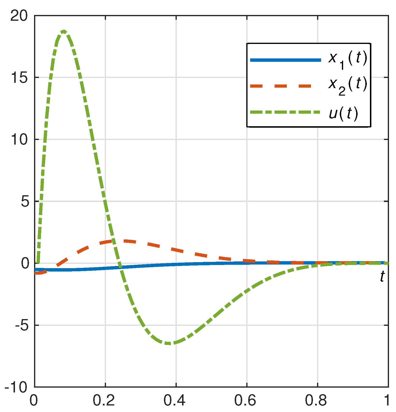
To demonstrate the algorithm, we considered a problem of controlling a single-link manipulator when transporting a load to a required position. According to [55], the manipulator motion in the presence of perturbations is described with the system

$$\left\{\begin{array}{cc}\hfill \dot{x_1}& =x_2,\hfill \\ \hfill \dot{x_2}& =-a_{2}sin{x}_1-a_1{x}_2+u(t-h)+g,\hfill \end{array}\right.$$

(56)

where $x_1$ is the angle of the manipulator deviation from the vertical, $x_2$ is the change rate of its deflection angle, $a_1=\overline{\alpha }{L}^{-2}{m}_1^{-1}$, $a_2=G{L}^{-1}\left(m_0+\frac{M}{2}\right)m_1^{-1}$, $m_1=m_0+\frac{M}{3}$, M is the manipulator’s mass, L is its length, G is the gravity constant, $\overline{\alpha }$ is the coefficient of viscous friction, $m_0$ is the mass of the load, and g as above is the perturbation. The vector of unknowns $x={(x_1,x_2)}^T$, and the control function u is applied only to ${\dot{x}}_2$. The boundary conditions are

$$\begin{array}{cccc}\hfill & x\left(0\right)=x^0,\hfill & \hfill & u\left(t\right)\equiv 0\mathrm{for}t\in [-h,0],\hfill \\ & \parallel x\left(t_{\epsilon }\right)\parallel \le \epsilon ,\hfill & \hfill & 1-t_{\epsilon }\le \epsilon .\hfill \end{array}$$

(57)

The system (10) and the conditions of Problem 2 read as

$$\begin{array}{cc}\hfill \frac{d{\xi }_1}{d\tau }& =\alpha e^{-\alpha \tau }{\xi }_2,\hfill \\ \hfill \frac{d{\xi }_2}{d\tau }& =-\alpha e^{-\alpha \tau }{a}_{2}sin{\xi }_1-\alpha e^{-\alpha \tau }{a}_1{\xi }_2+\alpha e^{-\alpha \tau }\upsilon +\alpha e^{-\alpha \tau }g,\hfill \end{array}$$

(58)

$$\begin{array}{cc}\hfill & {\xi }_1\left(0\right)=x_1^0,{\xi }_2\left(0\right)=x_2^0,\overline{\upsilon }\left(\tau \right)\equiv 0\mathrm{for}\tau \in \left[0,-\frac{1}{\alpha }ln(1-h)\right],\hfill \\ \hfill & \parallel {\xi }_1\left({\tau }_{\epsilon }\right)\parallel \le \epsilon ,\parallel {\xi }_2\left({\tau }_{\epsilon }\right)\parallel \le \epsilon ,e^{-\alpha {\tau }_{\epsilon }}\le \epsilon ,{\tau }_{\epsilon }>0.\hfill \end{array}$$

(59)

when applied to Problem (56), (57).

To solve Problem (58), (59) we make shifts (fewer than $4n=8$ suffice):

$$\begin{array}{cc}\hfill {\xi }_2\left(\tau \right)& ={\xi }_2^{\left(1\right)}\left(\tau \right)-e^{-\alpha \tau }g,\hfill \\ \hfill {\xi }_1\left(\tau \right)& ={\xi }_1^{\left(1\right)}\left(\tau \right)+\frac{1}{2}g{e}^{-2\alpha \tau },\hfill \\ \hfill {\xi }_2^{\left(1\right)}\left(\tau \right)& ={\xi }_2^{\left(2\right)}\left(\tau \right)+\frac{1}{2}g{a}_1{e}^{-2\alpha \tau },\hfill \\ \hfill {\xi }_1^{\left(1\right)}\left(\tau \right)& ={\xi }_1^{\left(2\right)}\left(\tau \right)+\frac{1}{6}g{a}_1{e}^{-3\alpha \tau },\hfill \\ \hfill {\xi }_2^{\left(2\right)}\left(\tau \right)& ={\xi }_2^{\left(3\right)}\left(\tau \right)-\frac{1}{6}g{a}_1{e}^{-3\alpha \tau }.\hfill \end{array}$$

Thus, with $\eta =({\xi }_1^{\left(2\right)},{\xi }_2^{\left(3\right)})$, the systems (20), (22) takes the form

$$\begin{array}{cc}\hfill \frac{d{\eta }_1}{d\tau }=& \alpha e^{-\alpha \tau }{\eta }_2-\frac{1}{6}\alpha a_{1}g{e}^{-4\alpha \tau },\hfill \\ \hfill \frac{d{\eta }_2}{d\tau }=& -\alpha e^{-\alpha \tau }{a}_1{\eta }_2+\alpha e^{-\alpha \tau }d+\frac{1}{6}\alpha e^{-4\alpha \tau }{a}_1^{2}g\hfill \\ \hfill & -\alpha e^{-\alpha \tau }{a}_{2}sin\left({\eta }_1+\frac{1}{6}g{a}_1{e}^{-3\alpha \tau }+\frac{1}{2}g{e}^{-2\alpha \tau }\right),\hfill \\ \hfill \frac{d\upsilon \left(\tau \right)}{d\tau }=& \omega .\hfill \end{array}$$

(60)

The linear part of system (60) is

$$\frac{d\overline{\eta }}{d\tau }=\overline{P}\overline{\eta }+\overline{Q}\upsilon ,\overline{\eta }={({\xi }_1^{\left(2\right)},{\xi }_2^{\left(3\right)},\upsilon )}^T,$$

(61)

$$\overline{P}=\left(\begin{array}{ccc}0& \alpha e^{-\alpha \tau }& 0\\ -\alpha e^{-\alpha \tau }{a}_2& -\alpha e^{-\alpha \tau }{a}_1& \alpha e^{-\alpha \tau }\\ 0& 0& 0\end{array}\right),\overline{Q}=\left(\begin{array}{c}0\\ 0\\ 1\end{array}\right).$$

According to [53], we obtain $\omega \left(\tau \right)=M\left(\tau \right)\overline{\eta }$, with $M\left(\tau \right)=(m_1,m_2,m_3)$,

$$\begin{array}{cc}\hfill m_1=& -e^{-\alpha \tau }{a}_1{a}_2\alpha +3a_2\alpha +6a_2-\frac{1}{{\alpha }^2}{e}^{2\alpha \tau }(8{\alpha }^3+24{\alpha }^2+22\alpha +6),\hfill \\ \hfill m_2=& -a_1^2\alpha +e^{-\alpha \tau }{a}_2\alpha +3a_1\alpha +6a_1-\frac{1}{\alpha }{e}^{\alpha \tau }(7{\alpha }^2+18\alpha +11),\hfill \\ \hfill m_3=& \alpha e^{-\alpha \tau }{a}_1-3\alpha -6,\hfill \end{array}$$

which stabilizes (61).

Now, we solve (60), closed by $\omega \left(\tau \right)$, with the initial values ${\eta }_1\left(0\right)=x_1^0-\frac{1}{2}g-\frac{1}{6}g{a}_1$, ${\eta }_2\left(0\right)=x_2^0+g-\frac{1}{3}g{a}_1$, $\upsilon \left(0\right)=0$. As a result, we obtain the way to compute $\omega \left(\tau \right)$, $\tau \in [0,+\infty )$. Substitution of (9) gives $w\left(t\right)=\omega \left(\tau \right(t\left)\right)$, $t\in [0,t_{\epsilon }]$.

Finally, we solve the initial value problem

$$\left\{\begin{array}{cc}\hfill \dot{x_1}& =x_2,\hfill \\ \hfill \dot{x_2}& =-a_{2}sin{x}_1-a_1{x}_2+u(t-h)+g,\hfill \\ \hfill \dot{u}& ={\alpha }^{-1}{(1-t)}^{-1}w\left(t\right)\hfill \end{array}\right.$$

$$x_1\left(0\right)=x_1^0,x_2\left(0\right)=x_2^0,u\left(t\right)\equiv 0\mathrm{for}t\in [-h,0]$$

over the interval $[0,t_{\epsilon }]$. The found functions $x_1\left(t\right)$, $x_2\left(t\right)$, and $u(t-h)$ solve Problem (56), (57).

We used Maplesoft Maple software for the experiment. It performed all the algebra, and we also solved the initial value problem using its default numerical ODE solver dsolve, which implemented a Runge–Kutta–Fehlberg pair of orders 5 and 4 with adaptive time-step, with default options, which were ${10}^{-7}$ for the absolute and ${10}^{-6}$ for the relative errors.

Figure 1 shows the solution for $x_1^0=-0.5$ rad, $x_2^0=-0.8$ rad/s, $\overline{\alpha }=0.1$, $L=10$ m, $M=20$ kg, $m_0=1$ kg, $\epsilon =0.05$, $t_{\epsilon }=0.9$ s, $g=0.1$, and $h=0.01$ s. The value $\alpha =0.25$ was chosen to be quite large to provide a small ${\tau }_{\epsilon }$ and still satisfy the constraint $\beta >0$ in (43).

7. Conclusions

We studied a class of nonlinear stationary controlled systems, which consider external perturbations and control delay.

The proposed method reduced the original problem to stabilizing an auxiliary system. Thus, it was possible to solve the original BVP problem taking into account errors in the initial values or other parameters and computational errors as well. The numerical test results demonstrated that the proposed method was applicable to the construction of control systems for different technical objects described by complex systems of differential equations. One of the main advantages of the presented approach is that the finite-time stabilization can be achieved even if the infinite-time stabilization is impossible.

Unfortunately, we were able to find other approaches to construct control functions only for linear or quasilinear systems with delays. There were no other algorithms for nonlinear systems with delays and perturbations. With the approach presented in the paper, we were able to construct Kalman-type stabilization criterion for systems without delays [56], so we will aim to apply it to delayed controls as well.

One of the problems with the suggested algorithm is that it uses analytic algebra, which makes it applicable only with special software and in case of a known right-hand side of (1). In addition, the presented results are local in the sense that the control may be found for sufficiently small initial points, delays, and perturbations.

One of the main future goals is to find less restrictive bounds for the initial values, perturbations, and delay that determine the attainability domain for the same Kalman-type condition (4). Furthermore, it is important to study if (4) is not only sufficient but also necessary. Another direction of research is to obtain the results for the stabilization problem with the stabilization condition (7) changed for $x\left(1\right)=0$.

References

- Elsisi, M.; Tran, M.Q.; Mahmoud, K.; Lehtonen, M.; Darwish, M.M.F. Robust design of ANFIS-based blade pitch controller for wind energy conversion systems against wind speed fluctuations. IEEE Access 2021, 9, 37894–37904. [Google Scholar] [CrossRef]
- Ning, X. Mixed sensitivity-based robust H∞ control method for real-time hybrid simulation. Symmetry 2021, 13, 840. [Google Scholar] [CrossRef]
- Elsisi, M.; Tran, M.Q.; Hasanien, H.M.; Turky, R.A.; Albalawi, F.; Ghoneim, S.S.M. Robust model predictive control paradigm for automatic voltage regulators against uncertainty based on optimization algorithms. Mathematics 2021, 9, 2885. [Google Scholar] [CrossRef]
- Huang, M.; Zhang, Z.; Wu, W.; Yao, Z. An improved three-level cascaded control for LCL-filtered grid-connected inverter in complex grid impedance condition. IEEE Access 2022, 10, 65485–65495. [Google Scholar] [CrossRef]
- Liu, K.; Xu, G.; Yang, Q.; Zhao, Z. Optimal disturbance suppression of disturbed underwater vehicle with state delay. IEEE Access 2022, 10, 63984–63990. [Google Scholar] [CrossRef]
- Prakash, A.; Kumar, K.; Parida, S. Energy capacitor system based wide-area damping controller for multiple inter-area modes. IEEE Trans. Ind. Appl. 2022, 58, 1543–1553. [Google Scholar] [CrossRef]
- Zhang, Z.; Min, X.; Chen, Y. An adaptive control scheme for data-driven traffic migration engineering on 5G network. Symmetry 2022, 14, 1105. [Google Scholar] [CrossRef]
- Arora, U.; Sukavanam, N. Approximate controllability of impulsive semilinear stochastic system with delay in state. Stoch. Anal. Appl. 2016, 34, 1111–1123. [Google Scholar] [CrossRef]
- Klamka, J. Stochastic controllability of linear systems with state delays. Int. J. Appl. Math. Comput. Sci. 2007, 17, 5–13. [Google Scholar] [CrossRef] [Green Version]
- Karthikeyan, S.; Sathya, M.; Balachandran, K. Controllability of semilinear stochastic delay systems with distributed delays in control. Math. Control Signals Syst. 2017, 29, 17. [Google Scholar] [CrossRef]
- Balachandran, K.; Balasubramaniam, P. A note on controllability of nonlinear Volterra integrodifferential systems. Kybernetika 1992, 28, 284–291. [Google Scholar]
- Sikora, B.; Klamka, J. Constrained controllability of fractional linear systems with delays in control. Syst. Control Lett. 2017, 106, 9–15. [Google Scholar] [CrossRef]
- Muni, V.S.; Govindaraj, V.; George, R.K. Controllability of fractional order semilinear systems with a delay in control. Indian J. Math. 2018, 60, 311–335. [Google Scholar]
- Chyung, D. On the controllability of linear systems with delay in control. IEEE Trans. Autom. Control 1970, 15, 255–257. [Google Scholar] [CrossRef]
- Sebakhy, O.; Bayoumi, M. A simplified criterion for the controllability of linear systems with delay in control. IEEE Trans. Autom. Control 1971, 16, 364–365. [Google Scholar] [CrossRef]
- Chyung, D. Controllability of linear time-varying systems with delays. IEEE Trans. Autom. Control 1971, 16, 493–495. [Google Scholar] [CrossRef]
- Olbrot, A. On controllability of linear systems with time delays in control. IEEE Trans. Autom. Control 1972, 17, 664–666. [Google Scholar] [CrossRef]
- Manitius, A.; Olbrot, A.W. Controllability conditions for linear systems with delayed state and control. Arch. Autom. Telemech. 1972, 17, 119–131. [Google Scholar]
- Sebakhy, O.; Bayoumi, M.M. Controllability of linear time-varying systems with delay in control. Int. J. Control 1973, 17, 127–135. [Google Scholar] [CrossRef]
- Zubov, V.I. Lectures in Control Theory; Nauka: Moscow, Russia, 1975. (In Russian) [Google Scholar]
- Klamka, J. Relative controllability of linear systems with varying delay. Syst. Sci. 1976, 2, 17–24. [Google Scholar]
- Klamka, J. Constrained controllability of second order dynamical systems with delay. Control Cybern. 2013, 42, 111–121. [Google Scholar]
- Olenchikov, D.M. Global controllability of sampled-data bilinear time-delay systems. J. Appl. Math. Mech. 2004, 68, 537–544. [Google Scholar] [CrossRef]
- Balachandran, K.; Balasubramaniam, P. Controllability of semilinear delay systems. Kybernetika 1994, 30, 517–524. [Google Scholar]
- Klamka, J. Constrained controllability of semilinear systems with delays. Nonlinear Dyn. 2009, 56, 169–177. [Google Scholar] [CrossRef]
- Klamka, J.; Czornik, A.; Niezabitowski, M.; Babiarz, A. Trajectory controllability of semilinear systems with delay. In Proceedings of the Intelligent Information and Database Systems, Bali, Indonesia, 23–25 March 2015; Nguyen, N.T., Trawiński, B., Kosala, R., Eds.; Springer: Cham, Switherland, 2015; pp. 313–323. [Google Scholar]
- Klamka, J. Controllability of nonlinear systems with delay in control. IEEE Trans. Autom. Control 1975, 20, 702–704. [Google Scholar] [CrossRef]
- Klamka, J. Relative controllability of nonlinear systems with delays in control. Automatica 1976, 12, 633–634. [Google Scholar] [CrossRef]
- Dauer, J.P.; Gahl, R.D. Controllability of nonlinear delay systems. J. Optim. Theory Appl. 1977, 21, 59–70. [Google Scholar] [CrossRef]
- Sinha, A.; Yokomoto, C. Null controllability of a nonlinear system with variable time delay. IEEE Trans. Autom. Control 1980, 25, 1234–1236. [Google Scholar] [CrossRef]
- Minyuk, S.A.; Lyakhovets, S.N. On the problem of controllability for systems with many delays. Vestsi Akad. Nauk BSSR. Ser. Fiz.-Mat. Navuk 1980, 2, 12–17. [Google Scholar]
- Dacka, C. Relative controllability of perturbed nonlinear systems with delay in control. IEEE Trans. Autom. Control 1982, 27, 268–270. [Google Scholar] [CrossRef]
- Balachandran, K.; Somasundaram, D. Controllability of a class of nonlinear systems with distributed delays in control. Kybernetika 1983, 19, 475–482. [Google Scholar]
- Somasundaram, D.; Balachandran, K. Relative controllability of a class of nonlinear systems with delay in control. Indian J. Pure Appl. Math. 1983, 14, 1327–1334. [Google Scholar]
- Somasundaram, D.; Balachandran, K. Controllability of nonlinear systems consisting of a bilinear mode with distributed delays in control. IEEE Trans. Autom. Control 1984, 29, 573–575. [Google Scholar] [CrossRef]
- Sinha, A.S.C. Null-controllability of non-linear infinite delay systems with restrained controls. Int. J. Control 1985, 42, 735–741. [Google Scholar] [CrossRef]
- Balachandran, K.; Somasundaram, D. Relative controllability of nonlinear systems with time varying delays in control. Kybernetika 1985, 21, 65–72. [Google Scholar]
- Balachandran, K. Controllability of nonlinear systems with delays in both state and control variables. Kybernetika 1986, 22, 340–348. [Google Scholar]
- Sinha, A.S.C. Controllability of non-linear delay systems. Int. J. Control 1986, 43, 1305–1315. [Google Scholar] [CrossRef]
- Balachandran, K.; Dauer, J. Controllability of perturbed nonlinear delay systems. IEEE Trans. Autom. Control 1987, 32, 172–174. [Google Scholar] [CrossRef]
- Balachandran, K. Complete controllability of nonlinear delay systems. IMA J. Math. Control Inf. 1987, 4, 161–166. [Google Scholar] [CrossRef]
- Balachandran, K. Global relative controllability of non-linear systems with time-varying multiple delays in control. Int. J. Control 1987, 46, 193–200. [Google Scholar] [CrossRef]
- Balachandran, K.; Dauer, J.P. Null controllability of nonlinear infinite delay systems with distributed delays in control. J. Math. Anal. Appl. 1990, 145, 274–281. [Google Scholar] [CrossRef] [Green Version]
- Dauer, J.; Balachandran, K.; Anthoni, S. Null controllability of nonlinear infinite neutral systems with delays in control. Comput. Math. Appl. 1998, 36, 39–50. [Google Scholar] [CrossRef] [Green Version]
- Golev, A.; Hristova, S.; Nenov, S. Monotone-iterative method for solving antiperiodic nonlinear boundary value problems for generalized delay difference equations with maxima. Abstr. Appl. Anal. 2013, 2013, 571954. [Google Scholar] [CrossRef]
- Kim, A.V.; Volkanin, L.S. On the synthesis of a control for systems with aftereffect in the control parameters. Izv. Ural. Gos. Univ. 2003, 26, 81–86. (In Russian) [Google Scholar]
- Thuan, M.V.; Trinh, H.; Huong, D.C. Reachable sets bounding for switched systems with time-varying delay and bounded disturbances. Int. J. Syst. Sci. 2017, 48, 494–504. [Google Scholar] [CrossRef]
- Klamka, J. Approximate controllability of delayed dynamical systems. Int. J. Appl. Math. Comput. Sci. 1997, 7, 5–16. [Google Scholar]
- Mouktonglang, T.; Poochinapan, K.; Yimnet, S. Robust finite-time control of discrete-time switched positive time-varying delay systems with exogenous disturbance and their application. Symmetry 2022, 14, 735. [Google Scholar] [CrossRef]
- Kvitko, A.N.; Firyulina, O.S.; Eremin, A.S. Solving boundary value problem for a nonlinear stationary controllable system with synthesizing control. Math. Probl. Eng. 2017, 2017, 8529760. [Google Scholar] [CrossRef] [Green Version]
- Kvitko, A.N.; Firyulina, O.S.; Eremin, A.S. Algorithm of the resolving of a boundary-value problem for a nonlinear controlled system and its numerical modeling. Vestn. St. Petersburg Univ. Math. 2017, 50, 372–383. [Google Scholar] [CrossRef]
- Kvitko, A.; Yakusheva, D. On one boundary problem for nonlinear stationary controlled system. Int. J. Control 2019, 92, 828–839. [Google Scholar] [CrossRef]
- Kvitko, A.N.; Maksina, A.M.; Chistyakov, S.V. On a method for solving a local boundary problem for a nonlinear stationary system with perturbations in the class of piecewise constant controls. Int. J. Robust Nonlinear Control 2019, 29, 4515–4536. [Google Scholar] [CrossRef]
- Barbashin, E.A. Introduction to Stability Theory; Wolters-Noordhof: Groningen, The Netherlands, 1970. [Google Scholar]
- Afanasiev, V.N.; Kolmanovskii, V.; Nosov, V.R. Mathematical Theory of Control Systems Design; Mathematics and Its Applications; Springer: Dordrecht, The Netherlands, 1996; Volume 341. [Google Scholar] [CrossRef]
- Kvitko, A.N. On a method for solving a local boundary value problem for a nonlinear stationary controlled system in the class of differentiable controls. Comput. Math. Math. Phys. 2021, 61, 527–541. [Google Scholar] [CrossRef]
Publisher’s Note: MDPI stays neutral with regard to jurisdictional claims in published maps and institutional affiliations. |
© 2022 by the authors. Licensee MDPI, Basel, Switzerland. This article is an open access article distributed under the terms and conditions of the Creative Commons Attribution (CC BY) license (https://creativecommons.org/licenses/by/4.0/).
Share and Cite
MDPI and ACS Style
Kvitko, A.N.; Eremin, A.S. A Constructive Method of Solving Local Boundary Value Problems for Nonlinear Systems with Perturbations and Control Delays. Symmetry 2022, 14, 1595. https://0-doi-org.brum.beds.ac.uk/10.3390/sym14081595
AMA Style
Kvitko AN, Eremin AS. A Constructive Method of Solving Local Boundary Value Problems for Nonlinear Systems with Perturbations and Control Delays. Symmetry. 2022; 14(8):1595. https://0-doi-org.brum.beds.ac.uk/10.3390/sym14081595
Chicago/Turabian StyleKvitko, Alexander N., and Alexey S. Eremin. 2022. "A Constructive Method of Solving Local Boundary Value Problems for Nonlinear Systems with Perturbations and Control Delays" Symmetry 14, no. 8: 1595. https://0-doi-org.brum.beds.ac.uk/10.3390/sym14081595
Note that from the first issue of 2016, this journal uses article numbers instead of page numbers. See further details here.