Article

Construction of General Implicit-Block Method with Three-Points for Solving Seventh-Order Ordinary Differential Equations

by
Mohammed Yousif Turki
1,
Mohammed Mahmood Salih
2 and
Mohammed S. Mechee
3,*
1
Department of Mathematics, College of Education for Pure Sciences, University of Anbar, Ramadi 31001, Iraq
2
College of Information Technology, Ninevah University, Mosel 41002, Iraq
3
Information Technology Research and Development Center (ITRDC), University of Kufa, Najaf 54006, Iraq
*
Author to whom correspondence should be addressed.
Submission received: 23 June 2022 / Revised: 21 July 2022 / Accepted: 27 July 2022 / Published: 4 August 2022
(This article belongs to the Special Issue Differential Equations and Applied Mathematics)

Abstract

:
In order to solve general seventh-order ordinary differential equations (ODEs), this study will develop an implicit block method with three points of the form y ( 7 ) ( ξ ) = f ( ξ , y ( ξ ) , y ( ξ ) , y ( ξ ) , y ( ξ ) , y ( 4 ) ( ξ ) , y ( 5 ) ( ξ ) , y ( 6 ) ( ξ ) ) directly. The general implicit block method with Hermite interpolation in three points (GIBM3P) has been derived to solve general seventh-order initial value problems (IVPs) using the basic functions of Hermite interpolating polynomials. A block multi-step method is constructed to be suitable with the numerical approximation at three points. However, the construction of the new method has been presented while the numerical results of the implementations are used to prove the efficiency and the accuracy of the proposed method which compared with the RK and RKM numerical methods together to analytical method. We established the characteristics of the proposed method, including order and zero-stability. Applications of various IVP problems are also discussed, and the outcomes are very encouraging for the suggested approach. The proposed GIBM3P method yields more accurate numerical solutions to the test problems than the existing RK method, which are in good agreement with analytical and RKM method solutions.

1. Introduction

Higher order differential equations (ODEs) have a significate role in various fields of applied mathematics and can be used in mathematical models problems that arise in the fields of applied sciences, biology, chemistry, physics, economics and engineering. Partial differential equations (PDEs) or ODEs are tools used to model the mathematical representations of the real problems in applied science and engineering. However, it had been difficult for mathematicians to use their creativity in finding the solutions of various types of DEs, either analytically or numerically. For scientists and engineers to use, there are currently a number of effective classical or modern numerical and analytical methods. The following list includes a review of the literature on various contemporary techniques for solving mathematical models that contain ODEs: for the purpose of solving IVPs, the numerical solutions of special and general sixth-order boundary-value problems (BVPs), with applications to Bénard layer eigenvalue problems, have been studied by researchers in [1], non-polynomial spline was used to solve BVPs by researchers in [2], while a new integrator was created in the research work [3] to solve ODEs of the seventh order. All types of DEs cannot always be solved directly or indirectly by analytical methods. This proposal would require us to research how direct GIBM3P is derived. However, the authors [4,5,6,7,8] have developed linear multistep numerical methods (Lmm) to address this issue, refs [9,10] have developed one-step numerical methods to solve IVPs of ODEs with orders lower than seven. Moreover, for future works, the studying of the authors [11,12,13] for the numerical solutions of a class of fractional order hybrid DEs and using the suggested technique, the oscillation of seventh-order neutral DEs can be modifided.
In this work, a new three-point second-derivative fully implicit block method has been proposed. The Hermite interpolating polynomial is used as the basis function to derive the implicit block method, which incorporates the first derivative of f ( ξ i , y i ( j ) ) for j = 0 , 1 , , 6 to enhance the accuracy of solutions. The novel contributions of this work are: to study the numerical solutions of seventh-order ODEs, to drive and construct a general implicit block with three-point GIBM3P method for solving ODEs of seventh-order, to use the numerical implementations to prove the efficiency and accuracy of the proposed GIBM3P method compared with the exact and numerical solutions and to apply the constructed method in solving some problems of ODEs of seventh-order comparing with the numerical solutions of RK and RKM methods. The derivatives are incorporated into the formula to produce more precise numerical results. To compare the effectiveness of the new method to numerical and exact solutions, a few numerical examples were evaluated. To obtain the numerical approximation at three points simultaneously, a block formulation is presented. IVPs applications are also discussed, and they produce impressive outcomes for the three-point block method suggested. The proposed GIBM3P method produces numerical results that are more precise than those produced by the current RK and RKM methods for test problems.

2. Preliminary

Definitions that are pertinent to this work are mentioned in this section.

2.1. The General Quasi-Linear Seventh-Order ODEs

The general quasi-linear seventh-order ODEs can be written in the following equation
y ( 7 ) ( ξ ) = f ( ξ , y ( ξ ) , y ( ξ ) , y ( ξ ) , y ( ξ ) , y ( 4 ) ( ξ ) , y ( 5 ) ( ξ ) , y ( 6 ) ( ξ ) ) ; ξ 0 ξ ξ 1 ,
with the following initial conditions:
y ( j ) ( ξ 0 ) = α j , j = 0 , 1 , , 6 .

Special Class Quasi-Linear Seventh-Order ODEs

The following form can be used to express the special class of seventh-order quasi-linear ODEs:
y ( 7 ) ( ξ ) = ϕ ( ξ , y ( ξ ) ) , ξ 0 ξ ξ 1 ,
with the initial conditions (ICs) in Equation (2).
Such ODEs are frequently found in many physical and engineering problems. Some scientists and engineers can solve the ODEs in Equation (1) or Equation (3) with ICs (2) using linear multistep methods. Most of them, used to solve higher order ODEs by converting the n t h -order ODE to equivalent first-order system of ODEs. However, it would be more efficient if ODEs of seventh-order in Equation (1) or Equation (3) with ICs (2) could be solved directly using the GIBM3P method which is more efficient since it has less function evaluations and computational time in implementation. In this paper, we are concerned with the implicit block method for solving seventh-order ODEs. Accordingly, we developed the order conditions for GIBM3P, so that based on the order conditions the GIBM3P method can be derived. By using Hermite polynomials as an approximation, the proposed method has been created.

2.2. RKM Methods for Solving Special Class Quasi-Linear Seventh-Order ODEs

RKM methods with s-stages developed by [3,14] proposed in this subsection for solving special quasi-linear seventh-order ODEs in Equation (3) with ICs (2) take the following form:
z n + 1 = z n + h z n + h 2 2 ! z n + h 3 3 ! z n + h 4 4 ! z n ( 4 ) + h 5 5 ! z n ( 5 ) + h 6 6 ! z n ( 6 ) + h 7 i = 1 s b i k i
z n + 1 = z n + h z n + h 2 2 ! z n + h 3 3 ! z n ( 4 ) + h 4 4 ! z n ( 5 ) + h 5 5 ! z n ( 6 ) + h 6 i = 1 s b i k i
z n + 1 = z n + h z n + h 2 2 ! z n ( 4 ) + h 3 3 ! z n ( 5 ) + h 4 4 ! z n ( 6 ) + h 5 i = 1 s b i k i
z n + 1 = z n + h z n ( 4 ) + h 2 2 ! z n ( 5 ) + h 3 3 ! z n ( 6 ) + h 4 i = 1 s b i k i
z n + 1 ( 4 ) = z n ( 4 ) + h z n ( 5 ) + h 2 2 ! z n ( 6 ) + h 3 i = 1 s b i k i
z n + 1 ( 5 ) = z n ( 5 ) + h z n ( 6 ) + h 2 i = 1 s b i k i
z n + 1 ( 6 ) = z n ( 6 ) + h i = 1 s b i k i
where,
k i = f ( x n + c i h , y n + h c i y n + h 2 2 c i 2 y n + h 3 6 c i 3 y n + h 4 24 c i 4 y n ( 4 ) + h 5 120 c i 5 y n ( 5 ) + h 6 720 c i 6 y n ( 6 ) + h 7 j = 1 i 1 a i j k j )
for i = 2 , 3 , , s . and h is the step-size.
The order conditions of the RKM method for solving special class sixth-order of quasi-linear ODEs have been derived by [10]. The parameters of RKM method’s, in Equations (4)–(11), are c i , a i j , b i ( k ) and are evaluated by resolving the system of algebraic order conditions, for i , j = 1 , 2 , , s and k = 0 , 1 , 2 , 3 , 4 , 5 , 6 . Table 1 displays Butcher Table for three-stage RKM integrators.

3. Analysis of Proposed GIBM3P Method for Solving General Quasi-Linear Seventh-Order ODEs

The derived method has been introduced in this section.

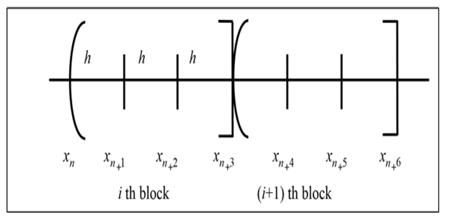
3.1. Proposed GIBM3P Method

Using the Hermite interpolating polynomial P 3 ( ξ ) , which is defined in the following equation, the new method is derived.
P 3 ( ξ ) = i = 0 n k = 0 m i 1 f i ( k ) L i , k ( ξ ) ,
where f i = f ( ξ i ) , ξ i = a + i h , i = 0 , 1 , and h = b a n , n is a positive integer. L i , k ( ξ ) can be defined by
L i , m i ( ξ ) = i , m i ( ξ ) , i = 0 , 1 , , n ,
i , k ( ξ ) = ( ξ ξ i ) k k ! j = 0 , j i n ( ξ ξ j ξ i ξ j ) m j , i = 0 , 1 , , n , k = 0 , 1 , , m i .
Furthermore, recursively for k = m i 2 , m i 3 , , 0 .
L i , k ( ξ ) = i , k ( ξ ) v = k + 1 m i 1 i , k ( v ) ( ξ i ) L i , v ( ξ ) .
For the purpose of directly solving the IVPs for the general class in Equation (1) or the special class in Equation (3) with ICs (2), a block method with some derivatives is developed in this paper. The derivation of the proposed method is based on the interpolating of Hermit polynomial denoted by P 3 ( t ) which interpolates at three points. This Hermit polynomial has the form in Equation (12) where, f i = f ( ξ i ) for j = 0 , 1 , , 6 and ξ i = a + i h ;   i = 0 , 1 , 2 , , m and h = b a m , where L i k ( ξ ) is the generalized Hermite polynomial for k = 0 , 1 , , m i and i = 0 , 1 , , m , where m is an integer’s positive. We use
P 3 ( ξ ) = f 0 L 00 ( ξ ) + f 1 L 10 ( ξ ) + f 2 L 20 ( ξ ) + f 3 L 30 ( ξ ) + f 0 L 01 ( ξ ) + f 1 L 11 ( ξ ) + f 2 L 21 ( ξ ) + f 3 L 31 ( ξ ) ,
where f = g ( ξ i , y i ( j ) ) is the derivative of the function f of order one with respect to ξ for j = 0 , 1 , , 6 and i = 0 , 1 , 2 , , m . The approximation at three points ξ m + 1 , ξ m + 2 and ξ m + 3 have computed the approximated solutions, y m + 1 , y m + 2 and y m + 3 , respectively, where ξ m = starting point and ξ m + 2 = ending point in the block [ ξ m , ξ m + 3 ] with step-size 3 h . The numerical solution y n + 3 at the ending point ξ m + 3 should be used as the initial value in the subsequent iteration, see Figure 1 which explains the block method with three points.

Hermite Polynomials

We used Hermite polynomials in this study, which are defined as follows:
L 00 ( ξ ) = 1 36 ξ 2 ( ξ + 1 ) 2 ( ξ + 2 ) 2 ( 1 + 11 3 ( ξ + 3 ) )
L 10 ( ξ ) = 1 4 ξ 2 ( ξ + 1 ) 2 ( ξ + 3 ) 3
L 20 ( ξ ) = 1 4 ξ 3 ( ξ + 2 ) 2 ( ξ + 3 ) 2
L 30 ( ξ ) = 1 36 ( ξ + 1 ) 2 ( ξ + 2 ) 2 ( ξ + 3 ) 2 ( 1 11 3 ξ )
L 01 ( ξ ) = h 36 ξ 2 ( ξ + 1 ) 2 ( ξ + 2 ) 2 ( ξ + 3 )
L 11 ( ξ ) = h 4 ξ 2 ( ξ + 1 ) 2 ( ξ + 2 ) ( ξ + 3 ) 2
L 21 ( ξ ) = h 4 ξ 2 ( ξ + 1 ) ( ξ + 2 ) 2 ( ξ + 3 ) 2
L 31 ( ξ ) = h 36 ξ ( ξ + 1 ) 2 ( ξ + 2 ) 2 ( ξ + 3 ) 2
Using the assumption s = ξ ξ n + 3 h , then, Hermite polynomials can be written in the independent variable ξ .

3.2. Derivation of Proposed GIBM3P Method

The three-point fully implicit block method with second derivatives was presented in this section as a solution to general seventh-order ODEs. The domain of definition [ a , b ] for this proposed method only has three points for each block. The approximated solution z n + 1 ( j ) , for j = 0 , 1 , 2 , 3 , 4 , 5 , 6 at the first point ξ n + 1 of Equation (12) can be obtained by integrating Equation (12) multiple times up to seventh-times with respect to the variable ξ , respectively, over the interval [ ξ m , ξ m + 1 ] . The integral formulas can be written as follows:
By integrating Equation (1), we get the following equations:
z n + 1 ( 6 ) = z n ( 6 ) + ξ n ξ n + 1 f ( Z ( ξ ) ) d ξ
z n + 1 ( 5 ) = z n ( 5 ) + h z n ( 6 ) + ξ n ξ n + 1 f ( Z ( ξ ) ) d ξ
z n + 1 ( 4 ) = z n ( 4 ) + h z n ( 5 ) + h 2 2 ! z n ( 6 ) + ξ n ξ n + 1 f ( Z ( ξ ) ) d ξ
z n + 1 ( 3 ) = z n ( 3 ) + h z n ( 4 ) + h 2 2 ! z n ( 5 ) + h 3 3 ! z n ( 6 ) + ξ n ξ n + 1 f ( Z ( ξ ) ) d ξ
z n + 1 = z n + h z n ( 3 ) + h 2 2 ! z n ( 4 ) + h 3 3 ! z n ( 5 ) + h 4 4 ! z n ( 6 ) + ξ n ξ n + 1 f ( Z ( ξ ) ) d ξ
z n + 1 = z n + h z n + h 2 2 ! z n ( 3 ) + h 3 3 ! z n ( 4 ) + h 4 4 ! z n ( 5 ) + h 5 5 ! z n ( 6 ) + ξ n ξ n + 1 f ( Z ( ξ ) )
z n + 1 = z n + h z n + h 2 2 ! z n + h 3 3 ! z n ( 3 ) + h 4 4 ! z n ( 4 ) + h 5 5 ! z n ( 5 ) + h 6 6 ! z n ( 6 ) + ξ n ξ n + 1 f ( Z ( ξ ) ) d ξ
where f ( Z ( ξ ) ) = f ( ξ , z ( j ) ( ξ ) ) for j = 0 , 1 , , 6 . Let ξ n + 1 = ξ n + h and the change of coordinate s = ξ ξ n + 3 h , d ξ = h d s where, f will be replaced by the following interpolating of Hermite polynomial in Equation (12), Θ ( s ) = f 0 L 00 ( s ) + f 1 L 10 ( s ) + f 2 L 20 ( s ) + f 3 L 30 ( s ) + g 0 L 01 ( s ) + g 1 L 11 ( s ) + g 2 L 21 ( s ) + g 3 L 31 ( s ) . Using the approximate concepts, the following formulas can be obtained:
z n + 1 ( 6 ) = z n ( 6 ) + 3 2 θ ( s ) h d s
z n + 1 ( 5 ) = z n ( 5 ) + h z n ( 6 ) 3 2 h ( 2 s ) Θ ( s ) h d s
z n + 1 ( 4 ) = z n ( 4 ) + h z n ( 5 ) + h 2 2 ! z n ( 6 ) + 3 2 ( h ( 2 s ) ) 2 2 ! θ ( s ) h d s
z n + 1 ( 3 ) = z n ( 3 ) + h z n ( 4 ) + h 2 2 ! z n ( 5 ) + h 3 3 ! z n ( 6 ) 3 2 ( h ( 2 s ) ) 3 3 ! θ ( s ) h d s
z n + 1 = z n + h z n ( 3 ) + h 2 2 ! z n ( 4 ) + h 3 3 ! z n ( 5 ) + h 4 4 ! z n ( 6 ) + 3 2 ( h ( 2 s ) ) 4 4 ! θ ( s ) h d s
z n + 1 = z n + h z n + h 2 2 ! z n ( 3 ) + h 3 3 ! z ( 4 ) + h 4 4 ! z n ( 5 ) + h 5 5 ! z n ( 6 ) + 3 2 ( h ( 2 s ) ) 5 5 ! θ ( s ) h d s
z n + 1 = z n + h z n + h 2 2 ! z n + h 3 3 ! z n ( 3 ) + h 4 4 ! z n ( 4 ) + h 5 5 ! z n ( 5 ) + h 6 6 ! z n ( 6 ) + 3 2 ( h ( 2 s ) ) 6 6 ! θ ( s ) h d s
By integration the Equations (28)–(34), we obtained the following new formulas:
z n + 1 ( 7 i ) = Δ i + h i ( a i 1 f 0 + a i 2 f 1 + a i 3 f 2 + a i 4 f 3 ) + h i + 1 ( a i 5 g 0 + a i 6 g 1 + a i 7 g 2 + a i 8 g 3 ) .
for i = 1 , 2 , , 7 , where
Δ i = j = 0 i 1 h j j ! z n ( 7 j ) ,
and
A = 6893 18144 313 672 89 672 397 18144 1283 30240 851 3360 269 3360 163 30240 19519 68040 1301 10080 181 2520 3329 272160 371 12960 313 2520 89 2016 137 45360 62387 544320 89 3360 439 20160 1031 272160 1879 181440 359 10080 13 960 17 18144 25883 816480 1457 332640 1579 332640 137 163296 3137 1197504 89 11880 283 95040 311 1496880 34673 5132160 325 532224 1091 1330560 10541 71850240 6163 11975040 3359 2661120 689 1330560 871 23950080 19607 16679520 73 988416 73 617760 259 12130560 9239 111196800 7723 43243200 103 1372800 589 111196800 186629 1077753600 293 37065600 7613 518918400 18719 7005398400 53329 4670265600 709 32432400 971 103783680 1549 2335132800
Evaluating the P 3 ( x ) at the point y n + 2 over [ x n + 1 , x n + 2 ] obtains a three-point fully implicit method. The second formula, y n + 2 , is obtained by using the same method as for the first formula, y n + 1
z n + 2 ( 7 i ) = Δ 7 + i + h i ( b i 1 f 0 + b i 2 f 1 + b i 3 f 2 + b i 4 f 3 ) + h i + 1 ( b i 5 g 0 + b i 6 g 1 + b i 7 g 2 + b i 8 g 3 ) .
for i = 1 , 2 , , 7 , where
Δ 7 + i = j = 0 i 1 h j j ! z n + 1 ( 7 j ) ,
and
B = 3 224 109 224 109 224 3 224 31 10080 113 1120 113 1120 31 10080 1921 272160 869 2520 1429 10080 431 68040 73 45360 121 2016 103 2520 19 12960 569 272160 533 4032 103 3360 941 544320 43 90720 19 960 103 10080 73 181440 73 163296 11819 332640 1777 332640 283 816480 151 1496880 443 45040 23 11880 97 1197504 5459 71850240 9869 1330560 2087 2661120 287 5132160 409 23950080 1151 1330560 799 2661120 157 11975040 131 12130560 157 123552 493 4942080 127 16679520 269 111196800 61 457600 1717 43243200 199 111196800 9281 7005398400 95987 518918400 2909 259459200 971 1077753600 691 2335132800 1829 103783680 149 32432400 991 4670265600
The purpose of evaluating the P 3 ( x ) at the point y n + 3 over [ x n + 2 , x n + 3 ] is to derive a three-point fully implicit method. By applying the same technique as for the first formula y n + 1 we have the third formula at x n + 3 :
z n + 3 ( 7 i ) = Δ 14 + i + h i ( c i 1 f 0 + c i 2 f 1 + c i 3 f 2 + c i 4 f 3 ) + h i + 1 ( c i 5 g 0 + c i 6 g 1 + c i 7 g 2 + c i 8 g 3 ) .
for i = 1 , 2 , , 7 , where
Δ 14 + i = j = 0 i 1 h j j ! z n + 2 ( 7 j ) ,
and
C = 397 18144 89 672 313 672 6893 18144 163 30240 269 3360 851 3360 1283 30240 1313 136080 611 10080 1697 5040 3617 38880 43 18144 181 5040 1301 10080 313 22680 151 60480 163 10080 2627 20160 107 6048 37 60480 19 2016 767 20160 89 30240 7 14580 1061 332640 1171 33264 2281 816480 703 5987520 61 33264 5477 665280 37 74844 299 3991680 41 80640 467 63360 3029 7983360 73 3991680 769 2661120 173 120960 557 7983360 331 33359040 113 1647360 521 411840 6047 133436160 269 111196800 53 1372800 287 1372800 3329 389188800 5359 4670265600 697 86486400 31891 172972800 11293 2335132800 29 103783680 389 8646400 4579 172972800 181 194594400

3.3. The Zero-Stability and the Order of the Proposed GIBM3P Method

The zero-stability and the order of the proposed GIBM3P method have been examined in this section.

3.3.1. Order of the GIBM3P Method

The three-point implicit block method’s formulas, which are given in Equations (35), (38) and (41) for i = 1 , 2 , , 7 , can be expressed in matrix form as follows:
α Y m = h β Y m + h 2 γ Y m + h 3 ψ Y m + h 4 δ Y m ( 4 ) + h 5 φ Y m ( 5 ) + h 6 λ Y m ( 6 ) + h 7 o F m + h 8 ρ G m
where, α , β , γ , ψ , δ , φ , λ , o and ρ are 21 × 21 matrices. We can define the linear operator as follows
L [ Z ( x ) ; h ] = α Y m h β Y m h 2 γ Y m h 3 ψ Y m h 4 δ Y m ( 4 ) φ h 5 F m h 6 λ h 7 o F m h 8 ρ G m .
Expanding Equation (44) using Taylor series at the point x where Z ( x ) is an arbitrary differentiable and continuous function.
L [ Z ( x ) ; h ] = C 0 Z ( x ) + C 1 h Z ( x ) + + C p h p Z p ( x ) + C p + 1 h p + 1 Z p + 1 ( x ) +
The linear operator of the proposed method in Equation (45) has order=p if C j = 0 for j = 0 , 1 , , p + 6 and C p + 7 0 . Where C p + 7 is the error constant. In the three-point implicit block method, we have C j = 0 ; j = 0 , 1 , , 14 . Therefore, the order of the three-point block method is eight.

3.3.2. Zero-Stability of the New Method

In this subsection, the zero-stability of the three-point fully implicit block method is studied. The formulas of the new method in Equations (35), (38) and (41) for i = 1 , 2 , , 7 are considered as a zero stable in case the roots r i = 1 , 2 , , N of the first characteristic polynomial ρ ( R ) = | R A ( 0 ) A ( 1 ) | = 0 are found to satisfy R 1 .
Moreover, in order to determine the matrix form of the first characteristic polynomial of the method, we will employ the following formulas. When the formulas in the Equations (35) and (38) are substituted for i = 1 , 2 , , 7 , we obtain
y n + 2 ( 6 ) = y n ( 6 ) + 223 h 567 f n + 20 h 21 f n + 1 + 13 h 21 f n + 2 + 20 h 567 f n + 3 + 43 h 2 945 g n 16 h 2 105 g n + 1 19 h 2 105 g n + 2 8 h 2 945 g n + 3
y n + 2 ( 5 ) = 2 h y n ( 6 ) + y n ( 5 ) + 5731 h 2 8505 f n + 296 h 2 315 f n + 1 + 109 h 2 315 f n + 2 + 344 h 2 8505 f n + 3 + 206 h 3 2835 g n 20 h 3 63 g n + 1 52 h 3 315 g n + 2 4 h 3 405 g n + 3
y n + 2 ( 4 ) = 2 h 2 y n ( 6 ) + 2 h y n ( 5 ) + y n ( 4 ) + 5048 h 3 8505 f n + 164 h 3 315 f n + 1 + 4 h 3 21 f n + 2 + 244 h 3 8505 f n + 3 + 172 h 4 2835 g n 4 h 4 15 g n + 1 34 h 4 315 g n + 2 4 h 4 567 g n + 3
y n + 2 = 4 3 h 3 y n ( 6 ) + 2 h 2 y n ( 5 ) + 2 h y n ( 4 ) + y n + 1804 h 4 5103 f n + 2168 h 4 10395 f n + 1 + 934 h 4 10395 f n + 2 + 376 h 4 25515 f n + 3 + 3224 h 5 93555 g n 7361909 h 5 53507520 g n + 1 16 h 5 297 g n + 2 68 h 5 18711 g n + 3
y n + 2 = 2 3 h 4 y n ( 6 ) + 4 3 h 3 y n ( 5 ) + 2 h 2 y n ( 4 ) + 2 h y n + y n + 44761 h 5 280665 f n + 692 h 5 10395 f n + 1 + 361 h 5 10395 f n + 2 + 236 h 5 40095 f n + 3 + 1391 h 6 93555 g n 592 h 6 10395 g n + 1 221 h 6 10395 g n + 2 136 h 6 93555 g n + 3
y n + 2 = 4 15 h 5 y n ( 6 ) + 2 3 h 4 y n ( 5 ) + 4 3 h 3 y n ( 4 ) + 2 h 2 y n + 2 h y n + y n + 2749 h 6 47385 f n + 344 h 6 19305 f n + 1 + 43 h 6 3861 f n + 2 + 200 h 6 104247 f n + 3 + 4502 h 7 868725 g n 196 h 7 10725 g n + 1 4652 h 7 675675 g n + 2 412 h 7 868725 g n + 3
y n + 2 = 4 45 h 6 y n ( 6 ) + 4 15 h 5 y n ( 5 ) + 2 3 h 4 y n ( 4 ) + 4 3 h 3 y n + 2 h 2 y n + 2 h y n + y n + 969008 h 7 54729675 f n + 8368 h 7 2027025 f n + 1 + 6152 h 7 2027025 f n + 2 + 2224 h 7 4209975 f n + 3 + 27688 h 8 18243225 g n 400 h 8 81081 g n + 1 3826 h 8 2027025 g n + 2 2384 h 8 18243225 g n + 3
Furthermore, by substituting Equations (46)–(52) into the formulas from the Equation (41) for i = 1 , 2 , , 7 , we get
y n + 3 ( 6 ) = y n ( 6 ) + 93 h 224 f n + 243 h 224 f n + 1 + 243 h 224 f n + 2 + 93 h 224 f n + 3 + 57 h 2 1120 g n 81 h 2 1120 g n + 1 81 h 2 1120 g n + 2 57 h 2 1120 g n + 3
y n + 3 ( 5 ) = 3 h y n ( 6 ) + y n ( 5 ) + 603 h 2 560 f n + 2187 h 2 1120 f n + 1 + 729 h 2 560 f n + 2 + 27 h 2 160 f n + 3 + 27 h 3 224 g n 243 h 3 560 g n + 1 234 h 3 1120 g n + 2 9 h 3 280 g n + 3
y n + 3 ( 4 ) = 9 2 h 2 y n ( 6 ) + 3 h y n ( 5 ) + y n ( 4 ) + 657 h 3 448 f n + 2187 h 3 1120 f n + 1 + 2187 h 3 2240 f n + 2 + 117 h 3 1120 f n + 3 + 351 h 4 2240 g n 729 h 4 1120 g n + 1 729 h 4 2240 g n + 2 27 h 4 1120 g n + 3
y n + 3 = 9 2 h 3 y n ( 6 ) + 9 2 h 2 y n ( 5 ) + 3 h y n ( 4 ) + y n + 27 h 4 20 f n + 16767 h 4 12320 f n + 1 + 729 h 4 1232 f n + 2 + 81 h 4 1120 f n + 3 + 3429 h 5 24640 g n 43938491 h 5 74910528 g n + 1 6561 h 5 24640 g n + 2 27 h 5 1540 g n + 3
y n + 3 = 27 8 h 4 y n ( 6 ) + 9 2 h 3 y n ( 5 ) + 9 2 h 2 y n ( 4 ) + 3 h y n + y n + 46251 h 5 49280 f n + 6561 h 5 8960 f n + 1 + 2187 h 5 7040 f n + 2 + 4293 h 5 98560 f n + 3 + 4617 h 6 49280 g n 579568537 h 6 1498210560 g n + 1 729 h 6 4480 g n + 2 1053 h 6 98560 g n + 3
y n + 3 = 81 40 h 5 y n ( 6 ) + 27 8 h 4 y n ( 5 ) + 9 2 h 3 y n ( 4 ) + 9 2 h 2 y n + 3 h y n + y n + 24003 h 6 45760 f n + 59049 h 6 183040 f n + 1 + 6561 h 6 45760 f n + 2 + 4023 h 6 183040 f n + 3 + 23247 h 7 457600 g n 705760183 h 7 3477988800 g n + 1 37179 h 7 457600 g n + 2 118669 h 7 21621600 g n + 3
y n + 3 = 81 80 h 6 y n ( 6 ) + 81 40 h 5 y n ( 5 ) + 27 8 h 4 y n ( 4 ) + 9 2 h 3 y n + 9 2 h 2 y n + 3 h y n + y n + 1571319 h 7 6406400 f n + 387099 h 7 3203200 f n + 1 + 373977 h 7 6406400 f n + 2 + 30213 h 7 3203200 f n + 3 + 5913 h 8 256256 g n 4992226654501 h 8 56385154425600 g n + 1 220887 h 8 6406400 g n + 2 1863 h 8 800800 g n + 3
The Equations (35), (46)–(59) for i = 1 , 2 , , 7 have now been substituted in order to determine the matrix and the first characteristic polynomial. The matrices’ general form is A ( i ) for i = 0 , 1 can be denoted by A ( 1 ) which is a matrix with all of its elements being zero, barring the following situations.
(i,j) ∈ {(1,15), (2,16), (3,17), (4,18), (5,19), (6,20), (7,21), (8,15), (9,16), (10,17), (11,18), (12,19), (13,20), (14,21), (15,15), (16,16), (17,17), (18,18), (19,19), (20,20), (21,21)} are all equal to one, where the Kroneker A ( 0 ) and A ( 1 ) are a 21 × 21 matrices.
Then, R 14 ( R 1 ) 7 = 0 , leads to R = 0 (14-times) and R = 0 (7-times). Hence, it can be concluded that the proposed method is zero stable.

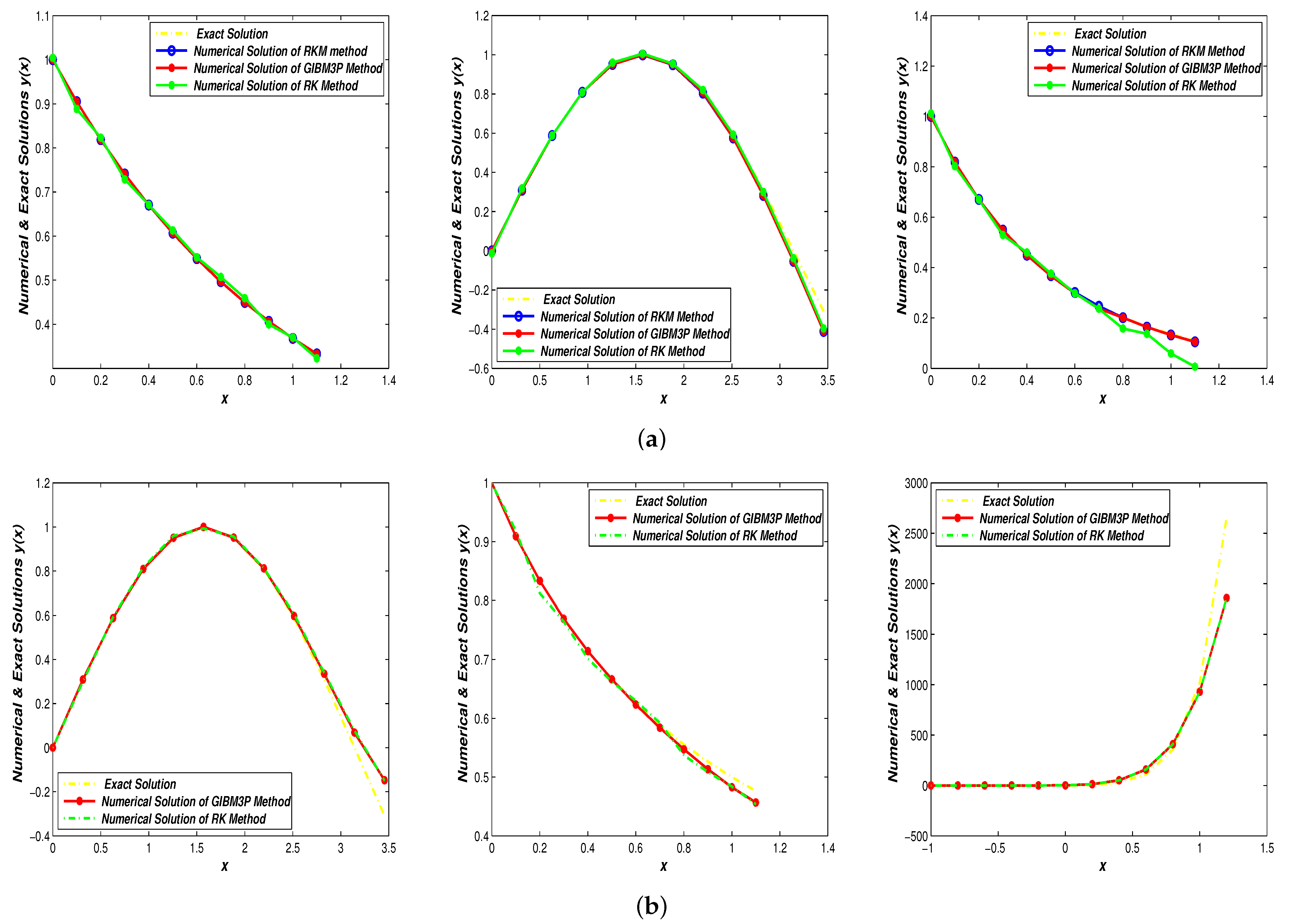
4. Numerical Implementations

The seventh-order GIBM3P method is used in this section to solve a collection of seventh-order ODEs. Figure 2 compares the numerical results to show the efficacy of the proposed method. The notations that were used are as follows:
  • RK Classical Runge–Kutta method.
  • RKM Direct Runge–Kutta–Mohammed method.
  • GIBM3P Proposed direct implicit block with three points method.

Problems Tested of ODEs

Example 1.
(Linear, non-homogenous ODE)
y ( 7 ) ( t ) = 2 y ( t ) + e t , 0 < t b .
  • Initial conditions, y ( i ) ( 0 ) = ( 1 ) i , i = 0 , 1 , , 6 .
  • Exact solution: y ( t ) = e t , b = 1 .
Example 2.
(Linear, homogenous ODE)
y ( 7 ) ( t ) = c o s ( t ) , 0 < t b .
  • Initial conditions, y ( 2 i + 1 ) ( 0 ) = ( 1 ) i , i = 0 , 1 , 2 ; y ( i ) ( 0 ) = 0 ; i = 0 , 2 , 4 , 6 .
  • Exact solution: y ( t ) = sin ( t ) , b = π .
Example 3.
(Non linear ODE)
y ( 7 ) ( t ) = y 4 ( t ) 128 y ( t ) e 8 t , 0 < t b .
  • Initial conditions, y ( 0 ) = 0 ; y ( i ) ( 0 ) = ( 1 ) i i ! ; i = 1 , , 6 .
  • Exact solution: y ( t ) = e 2 t , b = 1 .
Example 4.
(Homogenous ODE)
y ( 7 ) ( t ) = y ( t ) + y ( t ) + y ( t ) ; , 0 < t b .
  • Initial conditions, y ( 2 i + 1 ) ( 0 ) = ( 1 ) i , i = 0 , 1 , 2 ; y ( 2 i ) ( 0 ) = 0 , i = 0 , 1 , 2 , 3 .
  • Exact solution: y ( t ) = sin ( t ) , b = π
Example 5.
(Nonlinear ODE)
y ( 7 ) ( t ) = y 6 ( t ) + y 3 ( t ) 30 y 2 ( t ) , 0 < t b .
  • Initial conditions, y ( 0 ) = ( 1 ) i i ! , i = 0 , 1 , 2 , , 6 .
  • Exact solution: y ( t ) = 1 1 + t , b = 10
Example 6.
(Homogenous ODE)
y ( 7 ) ( t ) = y ( t ) + y ( t ) + 604800 ( 1 + t ) 3 + 10 ( 1 + t ) 8 ( 10 + t ) , 1 < t b .
  • Initial conditions, y ( i ) ( 0 ) = 0 , i = 0 , 1 , , 6 .
  • Exact solution: y ( t ) = ( 1 + t ) 10 , b = 1

5. Discussion and Conclusions

The general implicit block method with three points (GIBM3P) has been developed in this paper using the Hermite approximation method to solve a general class of seventh-order ODEs. The purpose of this article is to develop a direct-implicit block method for the general class of seventh-order ODEs. The proposed method has been numerically compared to direct RKM, existing RK methods, and exact solutions. This comparison leads us to the conclusion that the new method is accurate and effective. Based on the results of the implementations, we can say that the proposed method is more efficient than RK and RKM methods in terms of computation time while also requiring fewer function evaluations.

Author Contributions

Investigation, M.M.S.; Methodology, M.Y.T. and M.S.M.; Project administration, M.M.S.; Resources, M.M.S.; Software, M.Y.T.; Supervision, M.S.M.; Validation, M.Y.T.; Writing—original draft, M.S.M.; Writing—review and editing, M.S.M. All authors have read and agreed to the published version of the manuscript.

Funding

This research received no external funding.

Institutional Review Board Statement

Not applicable.

Informed Consent Statement

Not applicable.

Data Availability Statement

Not applicable.

Conflicts of Interest

The authors declare no conflict of interest.

References

  1. Twizell, E.; Boutayeb, A. Numerical methods for the solution of special and general sixth-order boundary-value problems, with applications to Bénard layer eigenvalue problems. Proc. R. Soc. Lond. A 1990, 431, 433–450. [Google Scholar]
  2. Akram, G.; Siddiqi, S.S. Solution of sixth order boundary value problems using non-polynomial spline technique. Appl. Math. Comput. 2006, 181, 708–720. [Google Scholar] [CrossRef]
  3. Mechee, M.S.; Mshachal, J.K. Derivation of embedded explicit RK type methods for directly solving class of seventh-order ordinary differential equations. J. Interdiscip. Math. 2019, 22, 1451–1456. [Google Scholar] [CrossRef]
  4. Turki, M.Y.; Alku, S.Y.; Mechee, M.S. The general implicit-block method with two-points and extra derivatives for solving fifth-order ordinary differential equations. Int. J. Nonlinear Anal. Appl. 2022, 13, 1081–1097. [Google Scholar]
  5. Allogmany, R.; Ismail, F. Direct Solution of u″ = f(t,u,u′) Using Three Point Block Method of Order Eight with Applications. J. King Saud-Univ.-Sci. 2021, 33, 101337. [Google Scholar] [CrossRef]
  6. Allogmany, R.; Ismail, F.; Majid, Z.A.; Ibrahim, Z.B. Implicit two-point block method for solving fourth-order initial value problem directly with application. Math. Probl. Eng. 2020, 2020, 6351279. [Google Scholar] [CrossRef]
  7. Allogmany, R.; Ismail, F. Implicit three-point block numerical algorithm for solving third order initial value problem directly with applications. Mathematics 2020, 8, 1771. [Google Scholar] [CrossRef]
  8. Turki, M.; Ismail, F.; Senu, N.; Ibrahim, Z.B. Direct integrator of block type methods with additional derivative for general third order initial value problems. Adv. Mech. Eng. 2020, 12, 1687814020966188. [Google Scholar] [CrossRef]
  9. Senu, N.; Mechee, M.; Ismail, F.; Siri, Z. Embedded explicit Runge–Kutta type methods for directly solving special third order differential equations y‴ = f(x,y). Appl. Math. Comput. 2014, 240, 281–293. [Google Scholar] [CrossRef]
  10. Mechee, M.S. Generalized RK integrators for solving class of sixth-order ordinary differential equations. J. Interdiscip. Math. 2019, 22, 1457–1461. [Google Scholar] [CrossRef]
  11. Jan, M.N.; Zaman, G.; Ahmad, I.; Ali, N.; Nisar, K.S.; Abdel-Aty, A.H.; Zakarya, M. Existence Theory to a Class of Fractional Order Hybrid Differential Equations. Fractals 2022, 30, 2240022. [Google Scholar] [CrossRef]
  12. Moaaz, O.; El-Nabulsi, R.A.; Muhib, A.; Elagan, S.K.; Zakarya, M. New Improved Results for Oscillation of Fourth-Order Neutral Differential Equations. Mathematics 2021, 9, 2388. [Google Scholar] [CrossRef]
  13. Cesarano, C.; Moaaz, O.; Qaraad, B.; Alshehri, N.A.; Elagan, S.K.; Zakarya, M. New Results for Oscillation of Solutions of Odd-Order Neutral Differential Equations. Symmetry 2021, 13, 1095. [Google Scholar] [CrossRef]
  14. Mechee, M.S.; Mshachal, J.K. Derivation of direct explicit integrators of RK type for solving class of seventh-order ordinary differential equations. Karbala Int. J. Mod. Sci. 2019, 5, 8. [Google Scholar] [CrossRef] [Green Version]
Figure 1. The block method with three points.
Symmetry 14 01605 g001
Figure 2. Numerical Solutions Using Proposed GIBM3P Method Versus (a) Classical RK method, RKM method and Analytical Solutions for Examples 1–3. (b) Classical RK method, and Analytical Solutions for Examples 4–6.
Symmetry 14 01605 g002
Table 1. Butcher table of RKM method.
00
3 5 6 10 1 2 0
3 5 + 6 10 1 2 1 2 0
10 119 120
1 40 6 360 1 60 + 6 360 0
1 18 1 18 6 48 1 18 + 6 48
1 9 7 36 6 48 7 18 6 18
1 9 7 36 6 48 7 18 6 18
Publisher’s Note: MDPI stays neutral with regard to jurisdictional claims in published maps and institutional affiliations.

