
Analysis of Adaptive Progressive Type-II Hybrid Censored Dagum Data with Applications


1
Department of Mathematical Sciences, College of Science, Princess Nourah bint Abdulrahman University, P.O. Box 84428, Riyadh 11671, Saudi Arabia
2
Department of Statistics, Faculty of Science, King Abdulaziz University, Jeddah 21589, Saudi Arabia
3
Department of Statistics, Faculty of Commerce, Zagazig University, Zagazig 44519, Egypt
4
Faculty of Technology and Development, Zagazig University, Zagazig 44519, Egypt
*
Author to whom correspondence should be addressed.
Symmetry 2022, 14(10), 2146; https://0-doi-org.brum.beds.ac.uk/10.3390/sym14102146
Submission received: 22 September 2022
/
Revised: 11 October 2022
/
Accepted: 12 October 2022
/
Published: 14 October 2022
(This article belongs to the Special Issue Symmetry in Statistics and Data Science)
Abstract
:In life testing and reliability studies, obtaining whole data always takes a long time and lots of monetary and human resources. In this case, the experimenters prefer to gather data using censoring schemes that make a balance between the length of the test, the desired sample size, and the cost. Lately, an adaptive progressive type-II hybrid censoring scheme is suggested to enhance the efficiency of the statistical inference. By utilizing this scheme, this paper seeks to investigate classical and Bayesian estimations of the Dagum distribution. The maximum likelihood and Bayesian estimation methods are considered to estimate the distribution parameters and some reliability indices. The Bayesian estimation is developed under the assumption of independent gamma priors and by employing symmetric and asymmetric loss functions. Due to the tough form of the joint posterior distribution, the Markov chain Monte Carlo technique is implemented to gather samples from the full conditional distributions and in turn obtain the Bayes estimates. The approximate confidence intervals and the highest posterior density credible intervals are also obtained. The effectiveness of the various suggested methods is compared through a simulated study. The optimal progressive censoring plans are also shown, and number of optimality criteria are explored. To demonstrate the applicability of the suggested point and interval estimators, two real data sets are also examined. The outcomes of the simulation study and data analysis demonstrated that the proposed scheme is adaptable and very helpful in ending the experiment when the experimenter’s primary concern is the number of failures.
Keywords:
Dagum distribution; adaptive progressive type-II hybrid censoring; likelihood estimation; Bayesian estimation; optimum progressive censoringMSC:
62F10; 62F15; 62N01; 62N02; 62N051. Introduction
The Dagum distribution offered by Dagum [1] has an essential role in modeling income distributions that could be utilized instead of some popular models including log-normal and Pareto models. Recently, authors have also considered the Dagum distribution in the context of reliability and survival analysis due to its flexibility for modeling lifetime data; see for example Domma et al. [2] and Emam and Sultan [3]. Presume that X is a lifetime random variable of an experimental item follows the three-parameter Dagum distribution, denoted by , where is the vector of the unknown parameters, with scale parameter and shape parameters and . Hence, the related probability density function (PDF) and the cumulative distribution function (CDF) of X, are given by
and
respectively. One can see that the Dagum distribution can be considered as a mixture model in terms of inverse Weibull and generalized gamma models. Kleiber and Kotz [4] and Kleiber [5] furnished a detailed appraisal of the core of the Dagum model as well as its applications. Further, two reliability indices of the Dagum distribution can be considered as unknown parameters, namely, reliability function (RF) and hazard rate function (HRF) at distinct time t which can be provided, respectively, by
and
The HRF of the Dagum distribution is either decreasing, upside-down, or a bathtub then upside-down bathtub. This appealing flexibility makes the HRF of the Dagum distribution meet appropriately even non-monotone HRF behaviors that are probable to be seen in a variety of domains. Different studies using the Dagum distribution have been achieved. Arif et al. [6] investigated the Bayesian estimation based on the Markov chain Monte Carlo (MCMC) technique. Naqash et al. [7] studied the Bayesian estimation of the scale parameter using different loss functions. Dey et al. [8] addressed different frequentist estimation methods for the unknown parameters. Alotaibi et al. [9] studied the Bayesian estimation using progressively type-I interval censored data. Kumari et al. [10] studied the classical and Bayesian estimation of the stress strength reliability using progressively type-II censored data.
Various censoring plans are known in the literature, which can be categorized into single-stage and multistage censoring schemes. Single-stage censoring schemes include type-I, type-II, and hybrid censoring. On the other hand, the most popular multistage censoring scheme is the progressive type-II censoring in which n units are placed on a test and m is a prefixed number of items to be failed with prefixed progressive censoring plan . At the time of the failure , surviving units are randomly removed from the test. At the time of the last failure , all the surviving units are removed. For further information about the progressive type-II censoring scheme, see Balakrishnan [11]. Kundu and Joarder [12] proposed a progressive type-I hybrid censoring scheme that has the same schematic representation as the progressive type-II censoring scheme but in this case, the test is stopped at , where T is a prefixed time.
The main drawback of this scheme is that the desired sample size is random and might turn out to be a very small number. As a consequence, the statistical deduction methods will be inadequate. To overpower this weakness, a more flexible censoring plan is proposed, namely an adaptive progressive type-II hybrid censoring (APT-II HC) scheme by Ng et al. [13]. In the APT-II HC, the experiment time is allowed to run over the time T and some values of conceivably revised during the test. If , the test stops at and we will retain the standard progressive type-II censoring. Otherwise, if , where and is the failure time occur before time T, then we will not remove any surviving units from the test by placing , and at the time of the last failure , all the remaining units are removed, i.e., . This adaption guarantees the ending of the test when we gather the desired number of failures m, and the total test time will not be too outlying from the ideal time T. Suppose that are an observed APT-II HC sample from a continuous population with PDF and CDF , then the likelihood function can be expressed as follows
where C is a constant that is independent of the parameters. Many works have been performed based on the APT-II HC scheme. Hemmati and Khorram [14] addressed the estimation of the competing risks model for the exponential distribution. Al Sobhi and Soliman [15] investigated the estimation issues of the exponentiated Weibull distribution. Nassar et al. [16] studied the classical and Bayesian estimation methods for the Weibull distribution. Panahi and Moradi [17] considered some estimations method for the inverted exponentiated Rayleigh distribution. Elshahhat and Nassar [18] studied the Bayesian estimation for the Hjorth distribution. See also the work of Kohansal and Shoaee [19], Panahi and Asadi [20], Ahmad et al. [21], Du and Gui [22], Ateya et al. [23], Alotaibi et al. [24,25], and Nassar et al. [26]. Recently, Elshahhat and Nassar [27] extended the APT-II HC scheme to binomial random removals.
We can motivate this study via (1) the significance of the APT-II HC scheme in increasing the efficiency of the statistical inference by avoiding getting small observed sample sizes. (2) The flexibility of the Dagum distribution in modeling different types of data sets with different HRF shapes including decreasing, upside-down, or a bathtub then an upside-down bathtub. As a result, we can list our objectives in this study as:
- (1)
- To explore the maximum likelihood estimators (MLEs) of the unknown parameters including the reliability measures as well as the associated approximate confidence intervals (ACIs).
- (2)
- To investigate the Bayes estimators and the highest posterior density (HPD) credible intervals. The Bayes estimators are acquired by using the MCMC method and by employing two loss functions, namely, squared error (SE) and general entropy (GE) loss functions.
- (3)
- It is not possible to judge which procedure provides the best estimates theoretically. Therefore, an extensive simulation study is implemented to study the behavior of the different estimates and make the comparison achievable.
- (4)
- To construct a guideline for picking the most appropriate estimation procedure for the Dagum distribution based on APT-II HC.
- (5)
- To determine the optimal progressive sampling plane for APT-II HC scheme in the case of Dagum distribution.
- (6)
- Because the applicability of the proposed methods is an important issue. The proposed methods are applied to investigate two real data sets.
The remainder of the paper is arranged as follows: The MLEs and ACIs are discussed in Section 2. The Bayes estimators and HPD credible intervals are considered in Section 3. Section 4 displays the outcomes of the simulation study. In Section 5, we provide various methods for choosing the best censoring plan. Section 6 investigates two applications for real data. Finally, Section 7 concludes the paper.
2. Frequentist Inference
Assume that are an APT-II HC sample of size m with taken from the Dagum distribution with PDF and CDF given, respectively, by (1) and (2). In this case, one can derive the likelihood function based on (1), (2), and (5), after ignoring the constant term, as follows
where for simplicity of notation. Practically, it is more convenient to work with the log-likelihood function rather than the likelihood function itself. Therefore, by taking the natural logarithm of the likelihood function in (6), the log-likelihood function can be written as
Let and denote MLEs of the unknown parameters , and , respectively. These estimators can be acquired by maximizing the objective function with respect to , and . An alternative approach to obtain the needed estimators is by solving the following three normal equations simultaneously
and
where . It is evident from the nonlinear equations in (8)–(10) that the MLEs of the unknown parameters and can not be obtained in explicit expressions. To overcome this problem, some numerical techniques can be implemented to obtain the MLEs in this case. Once the MLEs , and are obtained, we can utilize the invariance property of the MLEs to estimate the RF and HRF at a distinct time t. Employing the invariance property, the MLEs of the RF and HRF can be obtained using (3) and (4) as follow
Aside from obtaining the point estimates of the unknown parameters , and , it is also of interest to obtain the confidence intervals for these parameters. Here, we utilize the asymptotic properties of the MLEs to construct the ACIs of the unknown parameters as well as the reliability measures. It is known that based on the theory of large samples the asymptotic distribution of , where is the MLE of , is normal distribution with mean and variance–covariance matrix . Due to the complicated expressions of the Fisher information matrix, it is not easy to obtain such a variance–covariance matrix. In this case, we can consider to estimate , which can be acquired using the observed Fisher information matrix and given by
where
and
where
Presently, the ACIs of , and can be obtained as follows
where , and are the values obtained from (11), respectively, and is the upper percentile point of the standard normal distribution.
In addition to this, to construct the ACIs of the RF and HRF we need to obtain the variance of their estimators and . One of the most popular ways to approximate these variances is to apply the so-called delta method; see Greene [28] for more details. For example, to approximate the variance of , the delta method stated that, under some regularity conditions, the distribution of the statistics can be approximated by the normal distribution with mean and variance , where with the following elements
Thus, one can obtain the approximate estimate of variance of as , which is evaluated at the MLEs , and . Similarly, we can acquire the approximate estimate of variance of . Let , where
and
Hence, we can obtain the approximate estimate of variance of as , which is evaluated at the MLEs of the unknown parameters. Using the mentioned results, the two-sided ACIs for and at the confidence level are expressed, respectively, as
3. Bayesian Inference
This section derives the Bayesian estimators for the unknown parameters , and , as well as the and . In addition to the point estimates, the HPD credible intervals are studied. In the statistical investigation, the Bayesian technique has influential benefits over the maximum likelihood method because it delivers a natural path of combining prior information about the unknown parameters with new data within a solid theoretical framework.. The Bayesian technique is particularly usable in dependability studies and numerous other disciplines where data availability is a key barrier. This analysis explores the Bayesian estimation beneath the premise that the unknown parameters are independent and have gamma distributions, i.e., , , and . Based on these assumptions, the joint prior distribution of , and can be expressed as
where and , are the hyper-parameters and are always greater than zero. Combining the sample information provided by the likelihood function with the prior knowledge about the unknown parameters presented through the joint prior distribution and by applying the Bayes theorem, one can derive the posterior distribution of the unknown parameters , and . Therefore, from (6) and (12), the joint posterior distribution of and takes the form
where and A is the normalized constant. The loss function plays a critical role in Bayesian estimation because it can be used to identify overestimation and underestimation in the investigation. Here, we take into account the SE and GE loss functions. The SE loss function is one of the most often used symmetric loss functions, whereas the GE loss function is asymmetric. It is well known that the Bayes estimator in the case of the SE loss function is the posterior mean where the overestimation and underestimation are treated equally. Conversely, the GE loss function delivers diverse importance for overestimation and underestimation. The GE loss function introduced by Calabria and Pulcini [29] and defined as
where is the estimator of and is a parameter that determines the degree of asymmetry. The Bayes estimator of using GE loss function is given by
provided that exists and is finite.
It can be seen that when , the Bayes estimator in (14) coincides with the Bayes estimator under the SE loss function. Now, let any function of the unknown parameters, then the Bayes estimators based on the SE and GE loss functions can be obtained directly from (13), respectively, as follow
and
Clearly, calculating the Bayes estimators using (15) and (16) analytically are unattainable. As a result, we advocate employing the MCMC technique to obtain the Bayes estimates of , and and the associated HPD credible intervals. To apply the MCMC technique, we should first derive the full conditional distributions of , and . The required full conditional distributions can be given from (13) as follow
and
Nevertheless, it is noticeable that the full conditional posterior distributions of , and cannot be tended analytically to famous distributions. Consequently, it is not probable to generate samples straight by traditional techniques, whereas the plots of them indicate that they are equivalent to normal distribution. So, we need to induce the unknown parameters by employing Metropolis-–Hasting (MH) sampling. To involve the MH sampling, we assume the normal distribution as the proposal distribution to acquire the Bayesian estimates and to obtain the HPD credible intervals. The MH sampling functions as follows to generate samples from (17)–(19)
- Step 1.
- Put .
- Step 2.
- Set
- Step 3.
- Generate from the full conditional posterior distribution (17) using normal distribution, i.e., , and by applying the MH steps.
- Step 4.
- Step 5.
- Step 6.
- Set .
- Step 7.
- Redo steps 3–6, B times to obtain
To assure convergence and to withdraw the affection of the choice of starting values, the first Q generated variates are scrapped. In this case, we have , and . Based on large B, the generated sample forms an approximate posterior sample which can be employed to obtain the Bayes estimates and the HPD credible intervals. Now, let be the unknown parameter to be estimated. Then, the Bayes estimate of based on the SE loss function can be obtained as
Similarly, the Bayes estimate of based on the GE loss function can be computed as follows
On the other hand, to compute the HPD credible intervals of , , and , say , we order , as . Then, the two-sided HPD credible interval of becomes , where is specified such that
where denotes the largest integer less than or equal to . It is noteworthy to mention here that the results of Arif et al. [6] can be obtained as a special case of the results derived in this paper when , with , which is the complete sample case.
4. Monte Carlo Simulation
In this section, Monte Carlo simulations are performed to know the performance of the proposed estimators developed in the previous sections of the parameters, reliability, and hazard functions based on an APT-II HC scheme. First, we describe the simulation design. Then, some discussions regarding the simulation outcomes are reported.
4.1. Simulation Design
This subsection is devoted to how to conduct the proposed numerical study. First, we simulate 1000 APT-II HC samples from based on various choices of T (threshold time), n (total sample size), m (effective sample size) and (progressive censoring). Taking , the actual values of the reliability characteristics and are 0.043 and 0.371, respectively. Using T(=0.1, 0.5), n(=50,100) and m is specified as a percentage of n as (=50, 80)%, the proposed numerical experiments are performed. In addition, for each n and m, different removal patterns of the progressive type-II censoring mechanism, where is symbolized by (5.0*3.5), are used as
To simulate APT-II HC samples of size m from a given sample of size n with given progressive censoring , do the following steps:
- Step 1.
- Generate a conventional progressive type-II sample as
- (a)
- Generate from uniform distribution.
- (b)
- Put for
- (c)
- Set for . Hence, is a simulated progressive type-II sample of size m from the uniform distribution.
- (d)
- Set the progressive type-II from is generated.
- Step 2.
- Determine D and discard for .
- Step 3.
- Using truncated distribution , generate the first-order statistics of size .
In frequentist investigation, from the 1000 APT-II HC samples, the MLEs (along their 95% ACIs) of , , , , and are computed. In Bayesian analysis, to evaluate the effects of the priors, two informative sets of hyper-parameters are used; namely Prior-1: , and ; Prior-2: and . All hyper-parameter values associated with each unknown parameter are chosen in such a way that the prior average is equal to the expected value of the corresponding unknown parameter; see Kundu (2008). It is important to mention here that the frequentist methods may be better than the Bayes method because the latter is computationally more expensive if there is no prior information about the parameters of interest. A large 12,000 MCMC variates via MH sampler are generated and then the first 2000 variates are removed as burn-in period. Next, based on 10,000 MCMC variates, the average Bayes estimates of , , , , and using the SE and GE (for ) loss functions as well as the associated 95% HPD intervals are computed. The point estimates of the unknown parameters , , , , and (say for short), are compared using root-mean-squared errors (RMSEs) and mean relative absolute biases (MRABs) given, respectively, as
where is the number of replications and is the estimate of at the sample. In addition, the performance of the interval estimates is compared using their average confidence lengths (ACLs) and coverage percentages (CPs) delivered, respectively, by
where is the indicator function and and denote the lower and upper interval bounds, respectively.
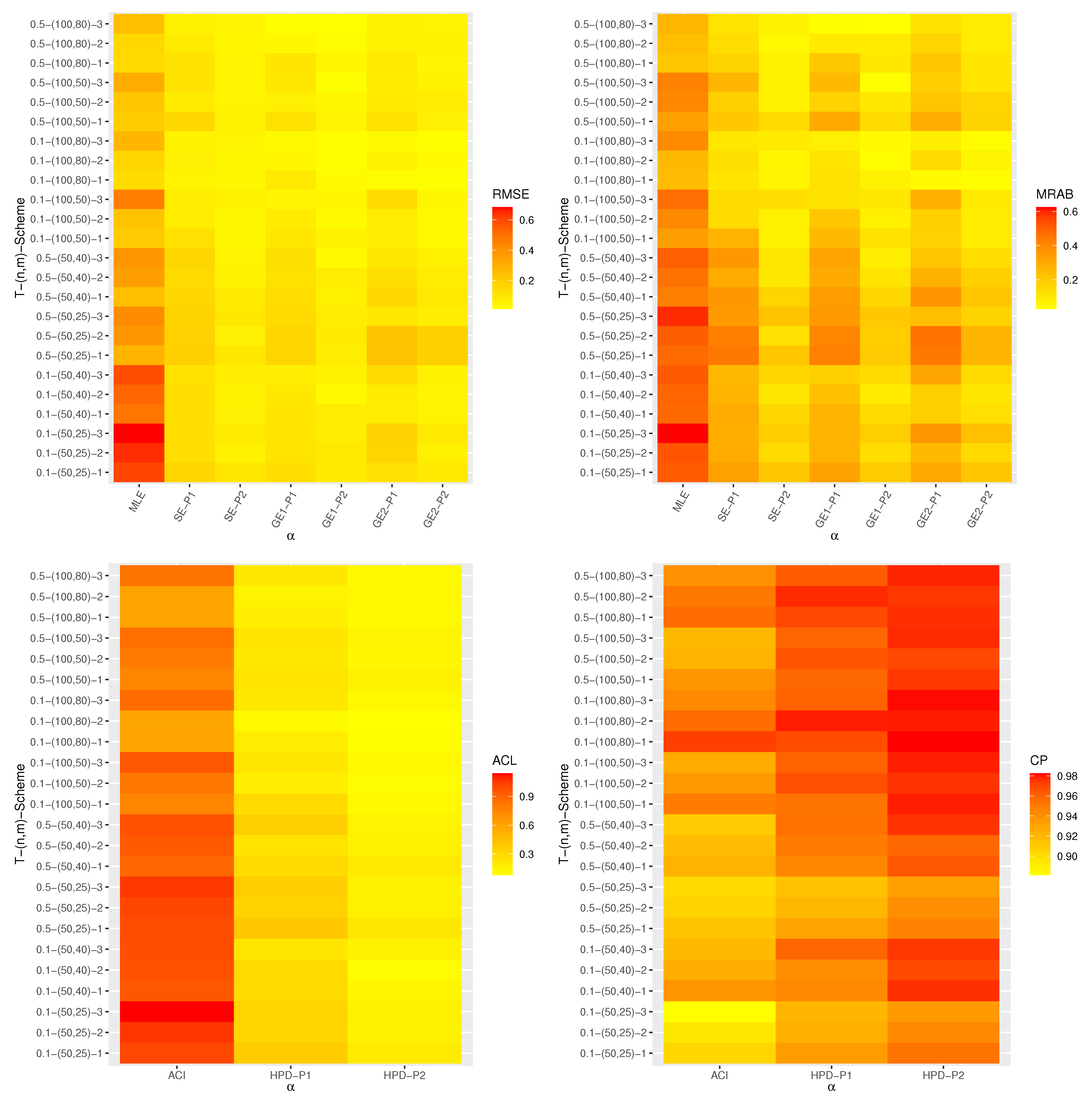
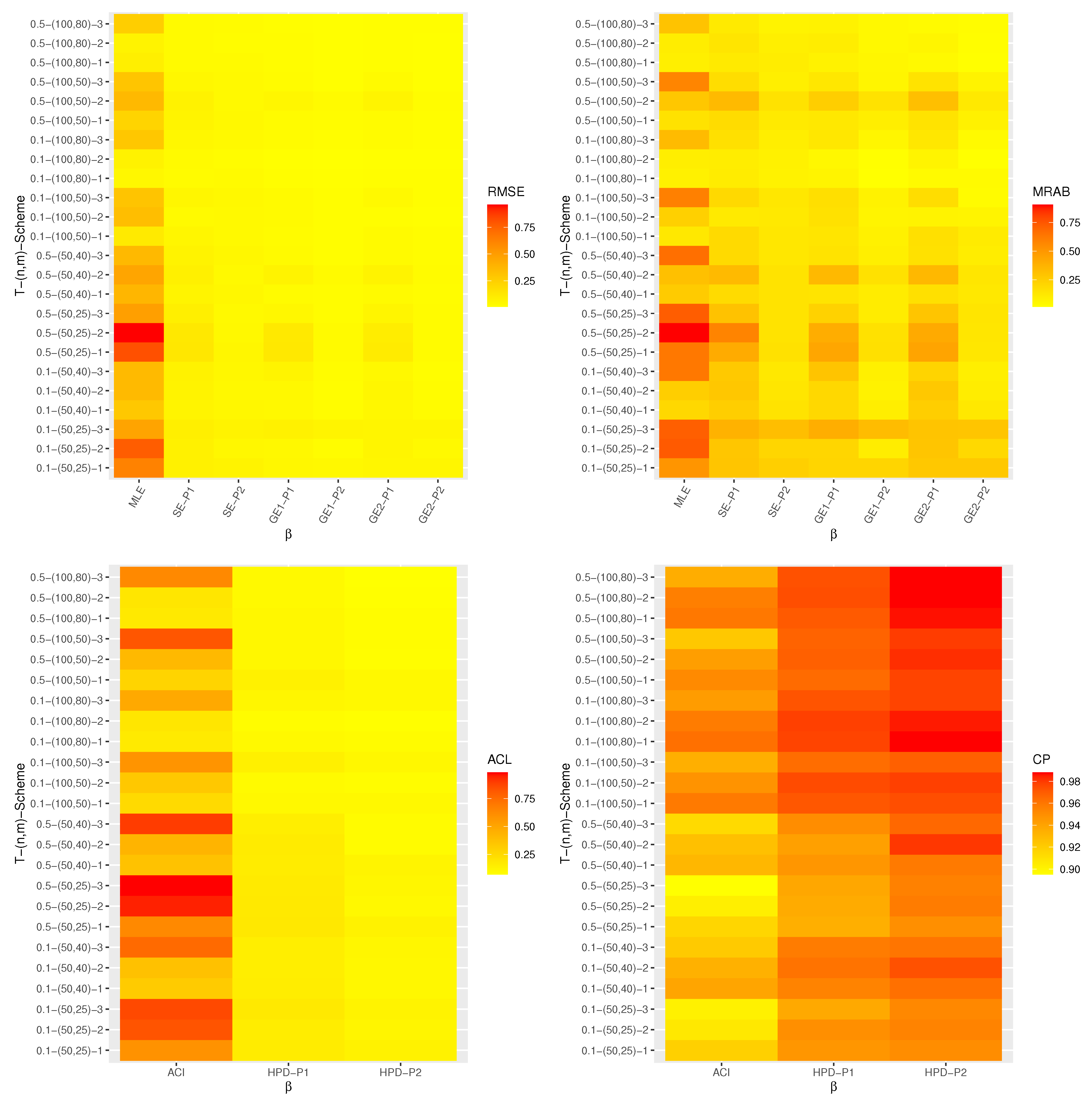
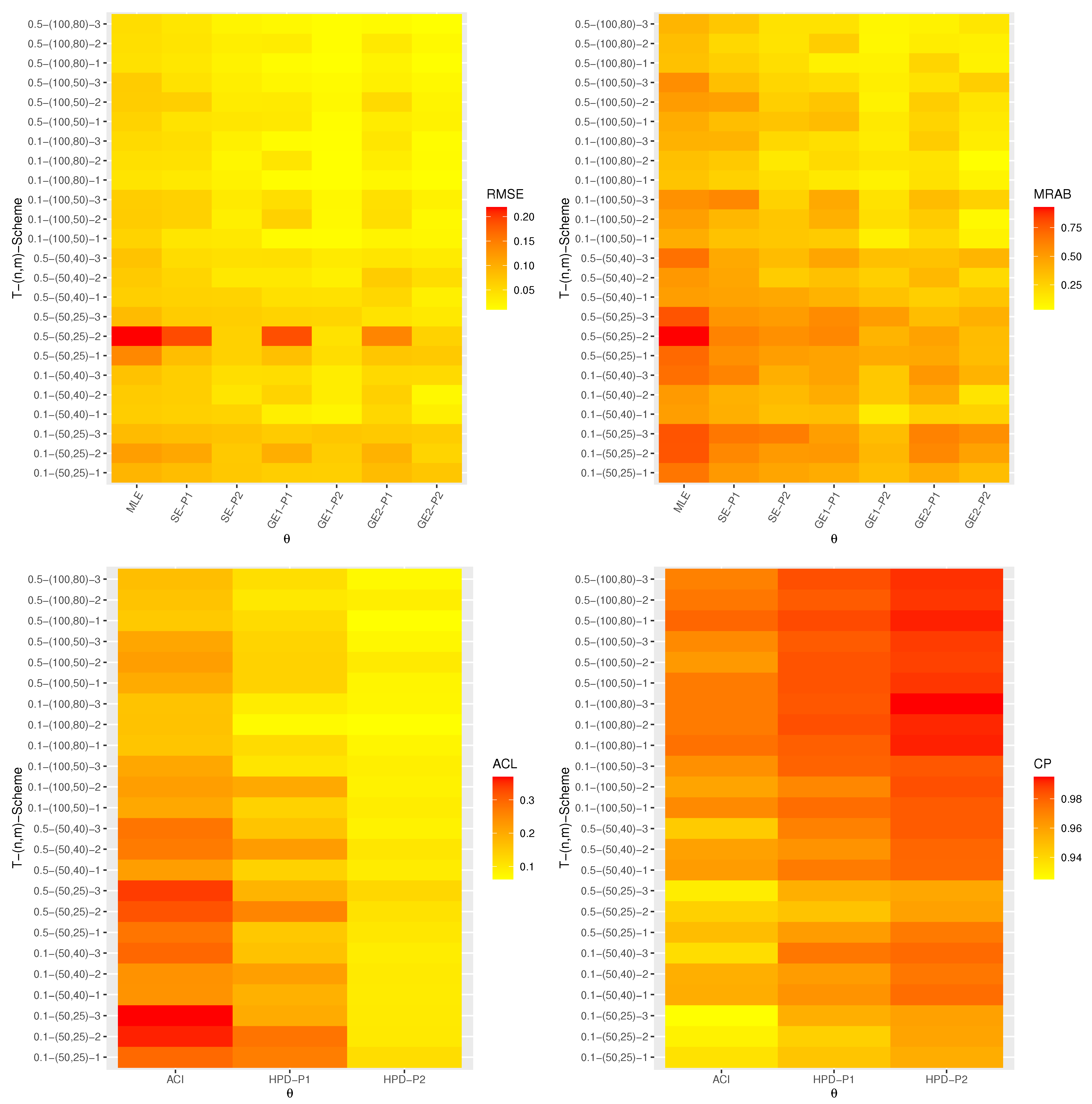
All calculations implemented are performed using 4.1.2 software by using two packages, namely (a) ‘coda’ (by Plummer et al. [30]) and (b) ‘maxLik’ (by Henningsen and Toomet [31]). These packages were also recommended by Elshahhat and Elemary [32]. Graphically, all simulation results of , , , , and are displayed with heatmap plots in Figure 1, Figure 2, Figure 3, Figure 4 and Figure 5, respectively, while all simulation outputs are provided as Supplementary Materials. In each heatmap, the ‘’ displays the proposed point (or interval) estimation methods while the ‘’ represents the given settings T, n, m, and , which are denoted by ‘T-()-Scheme’. For instance; based on Prior-1 set (say P1), we have used the notation “SE-P1” for the Bayes estimates from the SE loss; the notations “GE1-P1” and “GE2-P1” for the Bayes estimates from the GE loss based on and , respectively; “HPD-P1” denotes to HPD intervals. The color vector beside the heatmap represents the calculated values of the RMSEs, MRABs, ACLs, or CPs for each unknown parameter in each setting from lowest to highest value from yellow to red.
4.2. Simulation Discussions
Various appraisals of the performance of the proposed point and interval estimation methods are discussed in this subsection. From Figure 1, Figure 2, Figure 3, Figure 4 and Figure 5, the following observations can be made:
- All calculated estimates have displayed satisfactory behavior in terms of minimum RMSEs, MRABs, and ACLs values, as well as in terms of highest CPs.
- As n increases, the offered estimates are pretty satisfactory. Identical behavior is observed when (or ) lowers.
- As T increases, the RMSEs and MRABs for the MLEs of , , and decrease, while they increase for and . Moreover, as T increases, the RMSEs and MRABs of the Bayes estimates of , , and increase, while they decrease for and .
- As T increases, the ACLs of the ACIs of , , and decrease while they increase for and . Further, when T increases, the ACLs of the HPD interval estimates of , , and increase while they decrease for and . The opposite behavior is also observed in the case of the CPs for the ACI and HPD credible interval estimates of all unknown parameters.
- Since the Bayes estimates are expressed using the gamma density prior, the Bayes (point/interval) estimates using MH procedure perform better than the classical estimates in terms of the smallest RMSEs, MRABs, and ACLs as well as the highest CPs.
- It is also observed that the Bayes estimates based on Prior-2 are superior to Prior-1 for all unknown parameters. This is expected due to the fact that the variance of Prior-2 is smaller than Prior-1.
- It is noted that the CPs of the HPD intervals are almost closely (or greater) to the specified nominal level than the ACIs.
- It can be seen that the RMSEs, MRABs, ACLs, and CPs of , , , , and are even good based on Scheme-1 than other schemes.
- It is known that the expected duration of an experiment based on Scheme-1 is greater than that of any other, thus the APT-II HC sample gathered under this scheme supplied more additional information about the unknown parameters than those obtained based on any other censoring scheme.
- Overall, the Bayes procedure via MH algorithm is advised to estimate the unknown parameters of Dagum distribution and its reliability characteristics under the APT-II HC plan.
5. Optimal Progressive Censoring Plan
Choosing the optimal censoring plans has earned a lot of awareness in the statistical literature. For specified n and m, probable censoring schemes refer to all mixtures such that and picking the most suitable sample technique entails locating the progressive censoring scheme that delivers the most knowledge regarding the unknown parameters among all possible progressive censoring plans. For more details about optimal censoring plans, one can refer to Ng et al. [33] and Pradhan and Kundu [34]. In this study, we consider four optimality criteria that were widely used in the literature. Practically and as we mentioned before that we need to select the censoring scheme that provides us with the most information about the parameters. Table 1 furnishes some typically employed optimal criteria to aid us in choosing the most suitable progressive censoring scheme.
One can see from Table 1 that the criteria I, II, and III are looking for the progressive censoring scheme that maximize the observed Fisher information matrix, minimize the determinant of , and minimize the trace of , respectively. On the other hand, the criterion IV tries to minimize the variance of logarithmic MLE of the quantile, denoted by , where
where the delta method can be used to approximate the variance of . To pick the optimal progressive censoring plan, one should select the progressive censoring plan that gives the maximum value of criterion I and the smallest values of criteria II, III, and IV.
6. Real-Life Applications
To demonstrate how one can apply the proposed methodologies to a real-life situation, two applications using real-life data sets from chemistry and engineering areas are discussed in this section.
6.1. Coating Weights of Iron Sheets
In this application, from chemistry field, we shall provide a statistical analysis for the real coating weights of iron sheets obtained from the Aluminium Africa Limited (ALAF) industry, Tanzania, during January-March, 2018. To improve the quality of steel roofing, the coating process is one of the most processes used in this industry. Therefore, the ALAF industry uses the manufacturing technology of aluminum–zinc in the coating process. This data set consists of 72 observations on coating weight (in gm/m) by chemical method on top-center side from the ALAF industry; see Table 2. This data set was first discussed by Rao and Mbwambo [35] and also analyzed by Fan and Gui [36] recently.
To check whether the Dagum distribution is appropriate statistical distribution to fit the coating weight data set or not, the MLEs of the Dagum parameters , , and are calculated to carry out the Kolmogorov–Smirnov (K-S) distance and associated p-value. The values of , , and (with their standard errors (St.Es)) are 3163.52 (3.0251), 4.85561 (0.0329), and 16,655.9 (1.1860), respectively. The K-S (p-value) is 0.109 (0.364). This result indicates that the Dagum distribution is a proper lifetime model to fit the coating weight data. Moreover, using the complete coating weight data set, the estimated/empirical RF of the Dagum distribution is displayed in Figure 6.
From the original data set, three different APT-II HC samples are generated with and reported in Table 3. Based on the generated samples, the MLEs and Bayes estimates with their St.Es of , , , , and (at distinct time ) are computed and presented in Table 4. Additionally, the two bounds of 95% ACI/HPD intervals with their interval lengths (ILs) of the unknown parameters are also calculated and provided in Table 5. In order to develop the Bayes estimates, we assume that the hyper-parameters and for of , , , , and are not available. Therefore, to run our computations, the hyper-parameter values are selected to be 0.001. To run the MCMC algorithm, the classical estimates of , , and are taken to be the initial guesses. Table 4 and Table 5 indicated that the proposed Bayes estimates perform better than the frequentist estimates in terms of lowest St.Es, as well as, the HPD interval estimates also perform satisfactorily compared to the ACI estimates in terms of shortest ILs.
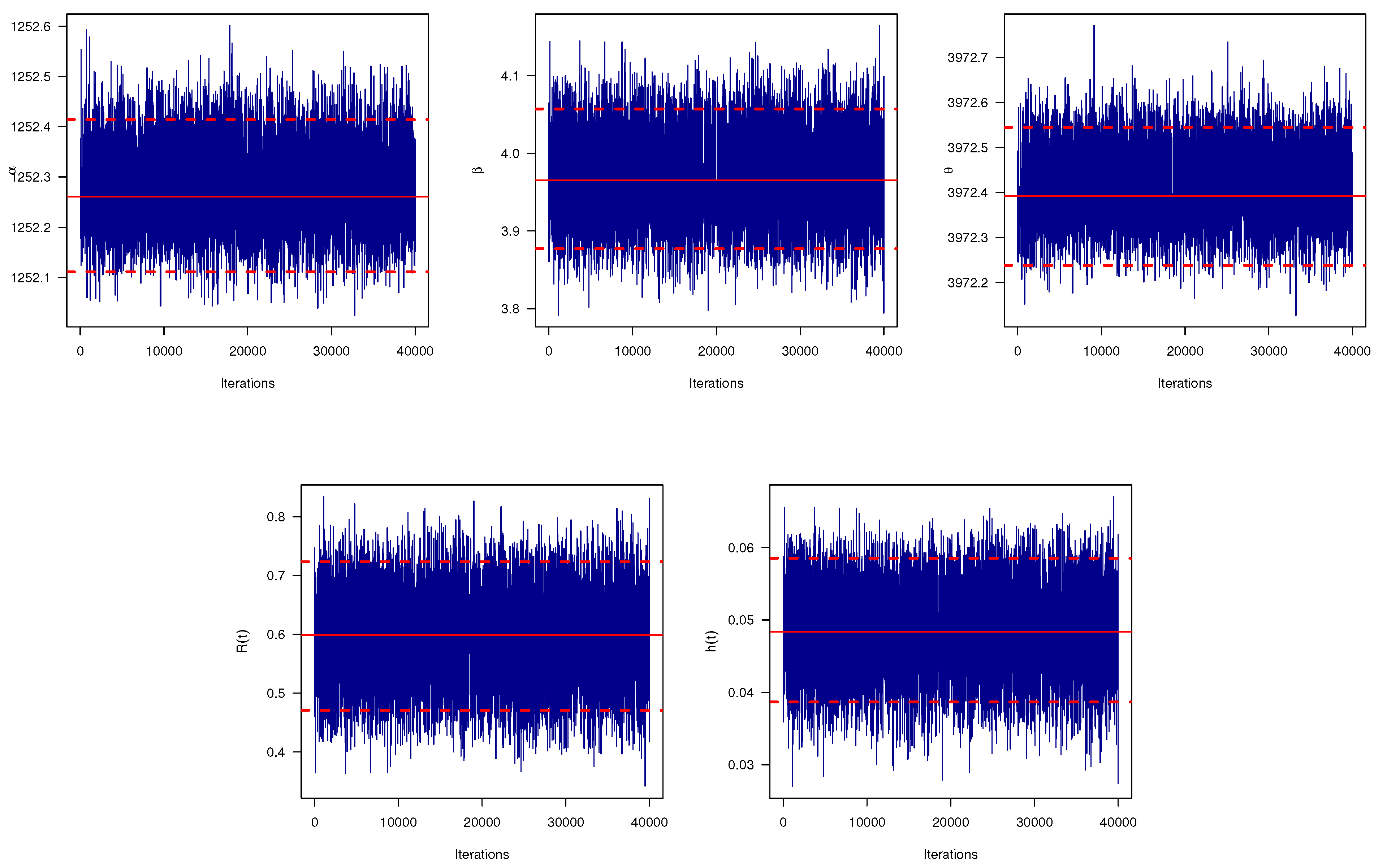
To show that the simulated MCMC samples are converged well, based on as an example, the trace plots based on 40,000 chain values of , , , , and are shown in Figure 7. Each trace plot represents the arithmetic sample mean (with solid (—) horizontal line) and two bounds of 95% HPD intervals (with dashed (- - -) horizontal line). It shows that the proposed MCMC algorithm converges well and the burn-in period has an appropriate size to ignore the effect of the starting guesses. Furthermore, based on as an example, the approximated marginal density functions with their frequencies using Gaussian kernel of , , , , and are displayed in Figure 8. It indicates that the simulated marginal posterior estimates of all the unknown parameters are fairly symmetrical. Furthermore, based on as an example, some general statistics for the MCMC outputs of , , , , and after burn-in, namely: mean, mode, mode, quartiles (), standard deviation (St.D), and skewness (Skew.) are also computed and presented in Table 6. Other MCMC plots based on samples and of , , , , and are plotted and reported in the Supplementary File for brevity. From Table 3, based on the four optimum criteria declared in Section 5, the problem of selecting the best (optimal) progressive censoring plan is discussed. The results of the different criteria are displayed in Table 7. It provides that the censoring scheme used in sample is the optimum plan based on the given criteria II, the censoring scheme used in sample is the optimum plan based on criterion I and III, and the censoring scheme used in sample is the optimum plan based on criterion IV.
6.2. Electronic Components
In this application, we use a real-life data set from the engineering field taken from Lawless [37]. This data set describes the failure times (in minutes) for a sample of fifteen electronic components in an accelerated life test as: 1.4, 5.1, 6.3, 10.8, 12.1, 18.5, 19.7, 22.2, 23, 30.6, 37.3, 46.3, 53.9, 59.8, 66.2. The MLEs of the unknown parameters are , , and . In addition, the K-S (p-value) is 0.107 (0.988). This result shows that the Dagum distribution fits the electronic components data set quite well. Furthermore, based on the electronic components data, the estimated/empirical RF of the Dagum distribution is displayed in Figure 9.
From the entire electronic components data set, by employing various censoring schemes, three APT-II HC samples with are generated and provided in Table 8. The different estimates of , , , , and are calculated and reported in Table 9 and Table 10, respectively. The estimates of and are evaluated at distinct time point . Again, by running the MCMC algorithm 50,000 times and discarding the first 10,000 estimates as burn-in, the Bayes estimates are obtained using the SE and GE (for ) loss functions.
It can be seen, from Table 9 and Table 10, that in terms of the lowest St.Es, the symmetric (or asymmetric) Bayes estimates of all unknown parameters perform better than the frequentist estimates. Moreover, in terms of the shortest interval width, the HPD interval estimates perform better than the ACIs.
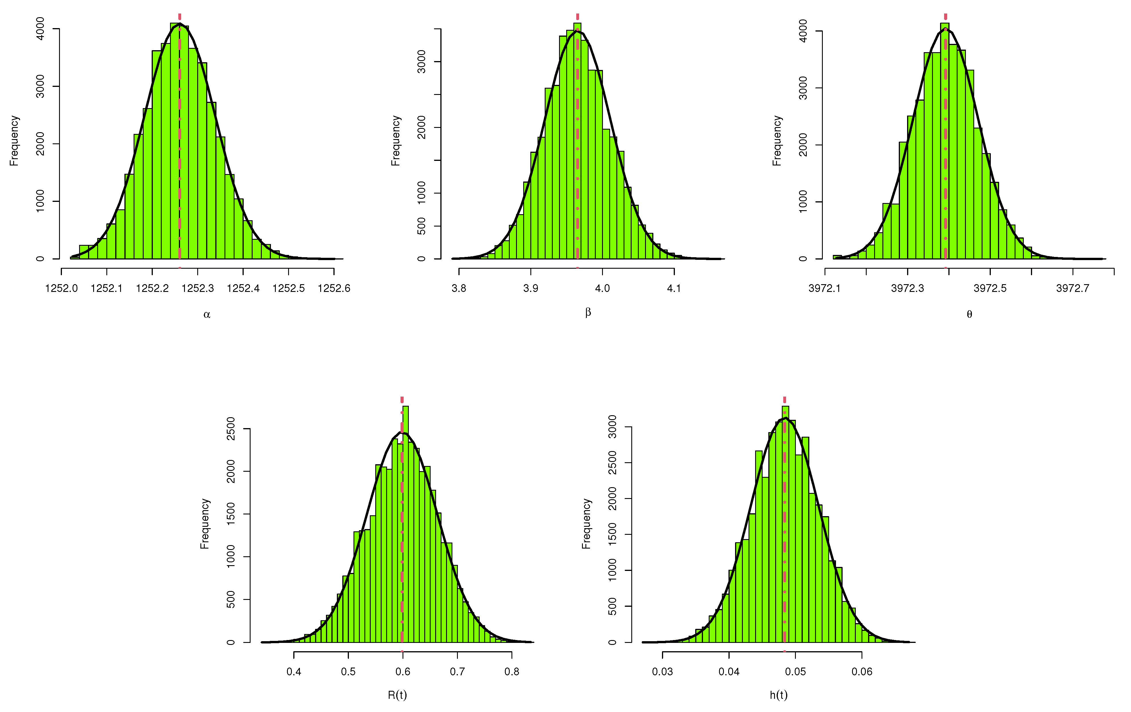
Utilizing the simulated 40,000 MCMC variates of , , , , and , their trace and histograms plots based on APT-II HC samples obtained from the electronic components data are plotted and displayed in Figure 10 and Figure 11, respectively. Figure 10 proves that the MCMC technique converges very well. In addition, Figure 11 shows that the distributions of the MCMC estimates of all unknown parameters are almost symmetric. Briefly, based on the simulated 40,000 MCMC variates of , , , , and from (as an example), some vital statistics called are calculated and listed in Table 11. In addition, the trace and histogram plots of the same unknown parameters based on samples and are also displayed in the Supplementary File.
In addition, using the optimum criteria reported in Section 5, the optimal progressive censoring mechanism is discussed. From the generated APT-II HC samples in Table 8, all optimum criteria are evaluated and presented in Table 12. It shows that the progressive type-II censoring plan used in is the optimum censoring than other competing schemes based on criteria I, II, and III while the progressive type-II censoring plan used in is the optimum censoring than others based on criterion IV for all specific percentile points.
7. Conclusions
In this study, based on an adaptive progressive type-II hybrid censoring scheme, we have attained the maximum likelihood and Bayes estimators of the unknown parameters, reliability, and hazard rate functions of the Dagum distribution. The Markov chain Monte Carlo approach is used to obtain the Bayes estimators based on squared error and general entropy loss functions. For the unknown parameters, reliability, and hazard rate functions, the approximative confidence intervals are obtained based on the asymptotic normality of the maximum likelihood estimators. In addition, the highest posterior density credible intervals are acquired. The optimal progressive censoring plans are shown and some optimality criteria are explored. A simulation study is used to examine the effectiveness of the various point and intervals estimators while taking various sample sizes and censoring strategies into account. The results of the simulation showed that the Bayesian approach offers estimates that are more accurate than the maximum likelihood approach. To demonstrate how the suggested estimators perform in real-world situations, we examined two actual data sets for coating weights of iron sheets and electronic components. The analysis showed that the Dagum distribution is a good choice to model these data and the Bayesian estimation method is advised to estimate the unknown parameters in the presence of adaptive progressively type-II hybrid censored Dagum data. For further research, the estimation of the reliability characteristics of the proposed model can be investigated by utilizing another estimation methods including the maximum product of spacing estimation method which may be a good alternative to the maximum likelihood method. Further, the methods developed in this paper can be extended to include the competing risks model or accelerated life tests.
Supplementary Materials
The following supporting information can be downloaded at: https://0-www-mdpi-com.brum.beds.ac.uk/article/10.3390/sym14102146/s1, Table S1: The APE (1st column), RMSEs (2nd column) and MRABs (3rd column) of ; Table S2: The APE (1st column), RMSEs (2nd column) and MRABs (3rd column) of ; Table S3: The APE (1st column), RMSEs (2nd column) and MRABs (3rd column) of ; Table S4: The APE (1st column), RMSEs (2nd column) and MRABs (3rd column) of ; Table S5: The APE (1st column), RMSEs (2nd column) and MRABs (3rd column) of ; Table S6: The ACLs (1st column) and CPs (2nd column) of 95% ACI/HPD intervals of ; Table S7: The ACLs (1st column) and CPs (2nd column) of 95% ACI/HPD intervals of ; Table S8: The ACLs (1st column) and CPs (2nd column) of 95% ACI/HPD intervals of ; Table S9: The ACLs (1st column) and CPs (2nd column) of 95% ACI/HPD intervals of ; Table S10: The ACLs (1st column) and CPs (2nd column) of 95% ACI/HPD intervals of ; Figure S1: Trace plots of , , , and using from coating weight data; Figure S2: Trace plots of , , , and using from coating weight data; Figure S3: Histograms of , , , and using from coating weight data; Figure S4: Histograms of , , , and using from coating weight data; Figure S5: Trace plots of , , , and using from electronic components data; Figure S6: Trace plots of , , , and using from electronic components data; Figure S7: Histograms of , , , and using from electronic components data; Figure S8: Histograms of , , , and using from electronic components data
Author Contributions
Methodology, H.S.M., R.A. and M.N.; Funding acquisition, H.S.M.; Software, A.E.; Supervision, H.S.M. and M.N.; Writing—original draft, M.N. and R.A.; Writing—review and editing, H.S.M., R.A., M.N. and A.E. All authors have read and agreed to the published version of the manuscript.
Funding
This research was funded by Princess Nourah bint Abdulrahman University Researchers Supporting Project number (PNURSP2022R175), Princess Nourah bint Abdulrahman University, Riyadh, Saudi Arabia.
Data Availability Statement
The authors confirm that the data supporting the findings of this study are available within the article.
Acknowledgments
The authors would desire to express their gratitude to the editor and the anonymous referees for useful advice and helpful comments.
Conflicts of Interest
The authors declare no conflict of interest.
References
- Dagum, C.A. New model for personal income distribution: Specification and estimation. Econ. Appl. 1977, 30, 413–437. [Google Scholar]
- Domma, F.; Giordano, S.; Zenga, M. Maximum likelihood estimation in Dagum distribution with censored samples. J. Appl. Stat. 2011, 38, 2971–2985. [Google Scholar] [CrossRef]
- Emam, W.; Sultan, K.S. Bayesian and maximum likelihood estimations of the Dagum parameters under combined-unified hybrid censoring. Math. Biosci. Eng. 2021, 18, 2930–2951. [Google Scholar] [CrossRef] [PubMed]
- Kleiber, C.; Kotz, S. Statistical Size Distributions in Economics and Actuarial Sciences; John Wiley & Sons: Hoboken, NJ, USA, 2003. [Google Scholar]
- Kleiber, C. A guide to the Dagum distribution, modeling income distributions and Lorenz curves economic studies in equality. Soc. Excl. Well-Being 2008, 5, 97–117. [Google Scholar]
- Arif, O.H.; Al-Shomrani, A.A.; Shawky, A.I. Analysis of Dagum Model for Software Reliability Using Markov Chain Monte Carlo Method. J. Comput. Theor. Nanosci. 2015, 12, 5153–5163. [Google Scholar] [CrossRef]
- Naqash, S.; Ahmad, S.P.; Ahmed, A. Bayesian analysis of Dagum distribution. J. Reliab. Stat. Stud. 2017, 10, 123–136. [Google Scholar]
- Dey, S.; Al-Zahrani, B.; Basloom, S. Dagum distribution: Properties and different methods of estimation. Int. J. Stat. Probab. 2017, 6, 74–92. [Google Scholar] [CrossRef]
- Alotaibi, R.; Rezk, H.; Dey, S.; Okasha, H. Bayesian estimation for Dagum distribution based on progressive type I interval censoring. PLoS ONE 2021, 16, e0252556. [Google Scholar] [CrossRef]
- Kumari, R.; Arora, S.; Mahajan, K.K. Estimation of stress-strength reliability for Dagum distribution based on progressive type-II censored sample. Model Assist. Stat. Appl. 2022, 17, 109–122. [Google Scholar] [CrossRef]
- Balakrishnan, N. Progressive censoring methodology: An appraisal (with discussions). Test 2007, 16, 211–296. [Google Scholar] [CrossRef]
- Kundu, D.; Joarder, A. Analysis of Type-II progressively hybrid censored data. Comput. Stat. Data Anal. 2006, 50, 2509–2528. [Google Scholar] [CrossRef]
- Ng, H.K.T.; Kundu, D.; Chan, P.S. Statistical Analysis of Exponential Lifetimes under an Adaptive Type-II Progressive Censoring Scheme. Nav. Res. Logist. 2009, 56, 687–698. [Google Scholar] [CrossRef] [Green Version]
- Hemmati, F.; Khorram, E. On adaptive progressively Type-II censored competing risks data. Commun. Stat. Simul. Comput. 2017, 46, 4671–4693. [Google Scholar] [CrossRef]
- Al Sobhi, M.M.A.; Soliman, A.A. Estimation for the exponentiated Weibull model with adaptive Type-II progressive censored schemes. Appl. Math. Model. 2016, 40, 1180–1192. [Google Scholar] [CrossRef]
- Nassar, M.; Abo-Kasem, O.; Zhang, C.; Dey, S. Analysis of Weibull distribution under adaptive Type-II progressive hybrid censoring scheme. J. Indian Soc. Probab. Stat. 2018, 19, 25–65. [Google Scholar] [CrossRef]
- Panahi, H.; Moradi, N. Estimation of the inverted exponentiated Rayleigh distribution based on adaptive Type II progressive hybrid censored sample. J. Comput. Appl. Math. 2020, 364, 112345. [Google Scholar] [CrossRef]
- Elshahhat, A.; Nassar, M. Bayesian survival analysis for adaptive Type-II progressive hybrid censored Hjorth data. Comput. Stat. 2021, 36, 1965–1990. [Google Scholar] [CrossRef]
- Kohansal, A.; Shoaee, S. Bayesian and classical estimation of reliability in a multicomponent stress-strength model under adaptive hybrid progressive censored data. Stat. Pap. 2021, 62, 309–359. [Google Scholar] [CrossRef]
- Panahi, H.; Asadi, S. On adaptive progressive hybrid censored Burr type III distribution: Application to the nano droplet dispersion data. Qual. Technol. Quant. Manag. 2021, 18, 179–201. [Google Scholar] [CrossRef]
- Haj Ahmad, H.; Salah, M.M.; Eliwa, M.S.; Ali Alhussain, Z.; Almetwally, E.M.; Ahmed, E.A. Bayesian and non-Bayesian inference under adaptive type-II progressive censored sample with exponentiated power Lindley distribution. J. Appl. Stat. 2022, 49, 2981–3001. [Google Scholar] [CrossRef]
- Du, Y.; Gui, W. Statistical inference of adaptive type II progressive hybrid censored data with dependent competing risks under bivariate exponential distribution. J. Appl. Stat. 2022, 49, 3120–3140. [Google Scholar] [CrossRef]
- Ateya, S.F.; Amein, M.M.; Mohammed, H.S. Prediction under an adaptive progressive type-II censoring scheme for Burr Type-XII distribution. Commun. Stat. Theory Methods 2022, 51, 4029–4041. [Google Scholar] [CrossRef]
- Alotaibi, R.; Nassar, M.; Elshahhat, A. Computational Analysis of XLindley Parameters Using Adaptive Type-II Progressive Hybrid Censoring with Applications in Chemical Engineering. Mathematics 2022, 10, 3355. [Google Scholar] [CrossRef]
- Alotaibi, R.; Elshahhat, A.; Rezk, H.; Nassar, M. Inferences for Alpha Power Exponential Distribution Using Adaptive Progressively Type-II Hybrid Censored Data with Applications. Symmetry 2022, 14, 651. [Google Scholar] [CrossRef]
- Nassar, M.; Alotaibi, R.; Dey, S. Estimation Based on Adaptive Progressively Censored under Competing Risks Model with Engineering Applications. Math. Probl. Eng. 2022, 2022, 6731230. [Google Scholar] [CrossRef]
- Elshahhat, A.; Nassar, M. Analysis of adaptive Type-II progressively hybrid censoring with binomial removals. J. Stat. Comput. Simul. 2022. [Google Scholar] [CrossRef]
- Greene, W.H. Econometric Analysis, 4th ed.; Prentice-Hall: New York, NY, USA, 2000. [Google Scholar]
- Calabria, R.; Pulcini, G. An engineering approach to Bayes estimation for the Weibull distribution. Microelectron. Reliab. 1994, 34, 789–802. [Google Scholar] [CrossRef]
- Plummer, M.; Best, N.; Cowles, K.; Vines, K. CODA: Convergence diagnosis and output analysis for MCMC. R News 2006, 6, 7–11. [Google Scholar]
- Henningsen, A.; Toomet, O. maxLik: A package for maximum likelihood estimation in R. Comput. Stat. 2011, 26, 443–458. [Google Scholar] [CrossRef]
- Elshahhat, A.; Elemary, B.R. Analysis for Xgamma Parameters of Life under Type-II Adaptive Progressively Hybrid Censoring with Applications in Engineering and Chemistry. Symmetry 2021, 13, 2112. [Google Scholar] [CrossRef]
- Ng, H.K.T.; Chan, C.S.; Balakrishnan, N. Optimal progressive censoring plans for the Weibull distribution. Technometrics 2004, 46, 470–481. [Google Scholar] [CrossRef]
- Pradhan, B.; Kundu, D. On progressively censored generalized exponential distribution. Test 2009, 18, 497–515. [Google Scholar] [CrossRef]
- Rao, G.S.; Mbwambo, S. Exponentiated inverse Rayleigh distribution and an application to coating weights of iron sheets data. J. Probab. Stat. 2019, 2019, 7519429. [Google Scholar] [CrossRef]
- Fan, J.; Gui, W. Statistical Inference of Inverted Exponentiated Rayleigh Distribution under Joint Progressively Type-II Censoring. Entropy 2022, 24, 171. [Google Scholar] [CrossRef]
- Lawless, J.F. Statistical Models and Methods for Lifetime Data, 2nd ed.; John Wiley and Sons: Hoboken, NJ, USA, 2011. [Google Scholar]
Figure 1.
Heatmap for the estimation results of .

Figure 2.
Heatmap for the estimation results of .

Figure 3.
Heatmap for the estimation results of .

Figure 4.
Heatmap for the estimation results of .

Figure 5.
Heatmap for the estimation results of .

Figure 6.
Plot of estimated/empirical Dagum reliability function from coating weight data.

Figure 7.
Trace plots of , , , , and using from coating weight data.

Figure 8.
Histograms of , , , , and using from coating weight data.

Figure 9.
Plot of estimated/empirical Dagum reliability function from electronic components data.

Figure 10.
Trace plots of , , , , and using from electronic components data.

Figure 11.
Histograms of , , , , and using from electronic components data.


Table 1.
Some optimal censoring plan criteria.
| Criterion | Method |
|---|---|
| I | |
| II | |
| III | |
| IV |
Table 2.
Coating weight data of iron sheets from ALAF industry.
| 28.7 | 29.4 | 30.4 | 31.6 | 31.8 | 32.7 | 32.9 | 33.2 | 33.2 | 33.6 | 33.7 | 34.0 | 34.2 | 34.5 | 35.6 |
| 36.2 | 36.7 | 36.8 | 36.8 | 37.3 | 37.8 | 38.5 | 38.9 | 38.9 | 39.1 | 39.9 | 40.1 | 40.2 | 40.3 | 40.5 |
| 40.6 | 40.7 | 41.2 | 41.2 | 41.3 | 42.3 | 42.3 | 42.6 | 42.8 | 42.8 | 42.8 | 42.8 | 43.1 | 44.2 | 44.9 |
| 45.2 | 45.3 | 45.4 | 45.8 | 46.3 | 47.1 | 47.2 | 47.2 | 48.2 | 48.3 | 48.4 | 48.5 | 49.8 | 50.1 | 52.6 |
| 52.8 | 54.2 | 54.5 | 55.4 | 55.8 | 56.8 | 58.2 | 58.4 | 58.7 | 58.9 | 59.2 | 61.2 |
Table 3.
Three APT-II HC samples from coating weight data.
| Sample | Scheme | T(D) | Data | ||||||||||
|---|---|---|---|---|---|---|---|---|---|---|---|---|---|
| 65(20) | 0 | 28.7 | 48.2 | 48.3 | 48.4 | 48.5 | 49.8 | 50.1 | 52.6 | 52.8 | 54.2 | ||
| 54.5 | 55.4 | 55.8 | 56.8 | 58.2 | 58.4 | 58.7 | 58.9 | 59.2 | 61.2 | ||||
| 45(11) | 12 | 28.7 | 29.4 | 30.4 | 31.6 | 31.8 | 32.7 | 32.9 | 33.2 | 36.8 | 40.5 | ||
| 42.8 | 47.2 | 47.2 | 48.2 | 48.3 | 48.4 | 48.5 | 49.8 | 50.1 | 52.6 | ||||
| 35(14) | 52 | 28.7 | 29.4 | 30.4 | 31.6 | 31.8 | 32.7 | 32.9 | 33.2 | 33.2 | 33.6 | ||
| 33.7 | 34.0 | 34.2 | 34.5 | 35.6 | 36.2 | 36.7 | 36.8 | 36.8 | 37.3 | ||||
Table 4.
Point estimates (St.Es) of , , , , and from coating weight data.
| Par. | MLE | SE | GE | |||
|---|---|---|---|---|---|---|
| +3 | ||||||
| 1252.3 (0.86) | 1252.2 (3.90) | 1252.2 (6.29) | 1252.3 (6.29) | 1252.26 (6.29) | ||
| 3.9852 (5.82) | 3.9653 (2.29) | 3.9658 (1.93) | 3.9650 (2.01) | 3.96423 (2.09) | ||
| 3972.5 (0.19) | 3972.4 (4.93) | 3972.4 (6.44) | 3972.4 (6.44) | 3972.38 (6.43) | ||
| 0.5697 (8.25) | 0.5985 (3.24) | 0.6055 (3.57) | 0.6054 (2.53) | 0.58368 (1.40) | ||
| 0.0507 (6.29) | 0.0484 (2.55) | 0.0489 (1.84) | 0.0481 (2.64) | 0.04724 (3.51) | ||
| 367.75 (0.88) | 367.69 (4.00) | 367.68 (6.22) | 367.69 (6.22) | 367.69 (6.23) | ||
| 2.8438 (3.63) | 2.8333 (1.62) | 2.8336 (1.02) | 2.8331 (1.07) | 2.8325 (1.13) | ||
| 165.34 (0.11) | 165.28 (4.02) | 165.27 (6.36) | 165.27 (6.37) | 165.27 (6.37) | ||
| 0.5194 (5.11) | 0.6065 (2.30) | 0.6099 (1.86) | 0.6048 (1.34) | 0.5993 (7.85) | ||
| 0.0351 (2.97) | 0.0342 (1.36) | 0.0344 (7.16) | 0.0341 (1.04) | 0.0338 (1.37) | ||
| 7887.5 (0.12) | 7887.4 (4.03) | 7887.4 (6.55) | 7887.4 (6.54) | 7887.4 (6.55) | ||
| 4.5696 (6.69) | 4.5453 (2.45) | 4.5458 (2.37) | 4.5450 (2.45) | 4.5442 (2.53) | ||
| 1060.1 (0.17) | 1060.1 (3.93) | 1060.1 (6.32) | 1060.1 (6.31) | 1060.1 (6.31) | ||
| 0.1342 (3.27) | 0.1486 (1.30) | 0.1532 (1.89) | 0.1464 (1.22) | 0.1394 (5.22) | ||
| 0.0850 (2.89) | 0.0838 (1.11) | 0.0838 (1.12) | 0.0837 (1.20) | 0.0836 (1.29) | ||
Table 5.
Interval estimates [ILs] of , , , , and from coating weight data.
| Par. | ACI | HPD | |
|---|---|---|---|
| 1252.3 (0.86) | 1252.2 (3.90) | ||
| 3.9852 (5.82) | 3.9653 (2.29) | ||
| 3972.5 (0.19) | 3972.4 (4.93) | ||
| 0.5697 (8.25) | 0.5985 (3.24) | ||
| 0.0507 (6.29) | 0.0484 (2.55) | ||
| 367.75 (0.88) | 367.69 (4.00) | ||
| 2.8438 (3.63) | 2.8333 (1.62) | ||
| 165.34 (0.11) | 165.28 (4.02) | ||
| 0.5194 (5.11) | 0.6065 (2.30) | ||
| 0.0351 (2.97) | 0.0342 (1.36) | ||
| 7887.5 (0.12) | 7887.4 (4.03) | ||
| 4.5696 (6.69) | 4.5453 (2.45) | ||
| 1060.1 (0.17) | 1060.1 (3.93) | ||
| 0.1342 (3.27) | 0.1486 (1.30) | ||
| 0.0850 (2.89) | 0.0838 (1.11) |
Table 6.
General MCMC statistics of , , , , and from coating weight data.
| Par. | Mean | Mode | St.D | Skew. | ||||
|---|---|---|---|---|---|---|---|---|
| 1252.261 | 1252.068 | 1252.209 | 1252.260 | 1252.313 | 0.078036 | 0.0244751 | ||
| 3.965291 | 3.907221 | 3.933091 | 3.963511 | 3.995504 | 0.045946 | 0.1275803 | ||
| 3972.392 | 3972.312 | 3972.338 | 3972.391 | 3972.445 | 0.078888 | 0.0201716 | ||
| 0.598523 | 0.681286 | 0.555022 | 0.600587 | 0.644260 | 0.064847 | −0.0823151 | ||
| 0.048374 | 0.041782 | 0.044874 | 0.048364 | 0.051859 | 0.005102 | −0.0849275 | ||
| 367.6869 | 367.4750 | 367.6337 | 367.6883 | 367.7404 | 0.080099 | −0.0316677 | ||
| 2.833264 | 2.812148 | 2.811808 | 2.855040 | 2.855040 | 0.032354 | 0.1253853 | ||
| 165.2781 | 165.1830 | 165.2245 | 165.2788 | 165.3317 | 0.080479 | −0.0474391 | ||
| 0.606512 | 0.636220 | 0.575109 | 0.608162 | 0.637130 | 0.046027 | −0.0984429 | ||
| 0.034195 | 0.032474 | 0.032423 | 0.034146 | 0.036066 | 0.002712 | −0.0080582 | ||
| 7887.434 | 7887.308 | 7887.379 | 7887.434 | 7887.489 | 0.080521 | 0.0109896 | ||
| 4.545287 | 4.553952 | 4.512051 | 4.543179 | 4.577726 | 0.049014 | 0.1251338 | ||
| 1060.076 | 1060.059 | 1060.024 | 1060.075 | 1060.129 | 0.078500 | 0.0402300 | ||
| 0.148638 | 0.130289 | 0.130289 | 0.147680 | 0.165139 | 0.026099 | 0.3562451 | ||
| 0.083788 | 0.084280 | 0.082341 | 0.083795 | 0.085312 | 0.002221 | −0.1591992 |
Table 7.
Optimal progressive censoring mechanisms from coating weight data.
| Sample | Criteria | |||||
|---|---|---|---|---|---|---|
| I | II | III | IV | |||
| 0.3 | 0.6 | 0.9 | ||||
| 295.8274 | 78.24976 | 0.931561 | 6.509199 | 11.16921 | 29.74584 | |
| 783.6007 | 78.78461 | 0.114358 | 4.650042 | 9.907341 | 38.79528 | |
| 223.3804 | 422.2169 | 88.67801 | 2.526266 | 4.086085 | 9.771803 | |
Table 8.
Three APT-II HC samples from electronic components data.
| Sample | Scheme | Data | |||||||||||
|---|---|---|---|---|---|---|---|---|---|---|---|---|---|
| 25(4) | 0 | 1.4 | 19.7 | 22.2 | 23 | 30.6 | 37.3 | 46.3 | 53.9 | 59.8 | 66.2 | ||
| 20(5) | 2 | 1.4 | 5.1 | 6.3 | 12.1 | 19.7 | 23 | 30.6 | 37.3 | 46.3 | 53.9 | ||
| 15(5) | 5 | 1.4 | 5.1 | 6.3 | 10.8 | 12.1 | 18.5 | 19.7 | 22.2 | 23 | 30.6 | ||
Table 9.
Point estimates (St.Es) of , , , , and from electronic components data.
| Par. | MLE | SE | GE | |||
|---|---|---|---|---|---|---|
| +3 | ||||||
| 0.6295 (2.22) | 0.5344 (4.29) | 0.5478 (8.17) | 0.5275 (1.02) | 0.5042 (1.25) | ||
| 2.2722 (1.81) | 2.1870 (4.15) | 2.1901 (8.20) | 2.1854 (8.67) | 2.1807 (9.15) | ||
| 4610.6 (0.11) | 4610.5 (4.89) | 4610.4 (9.74) | 4610.5 (9.74) | 4610.5 (9.73) | ||
| 0.6797 (1.13) | 0.6546 (3.37) | 0.6614 (1.83) | 0.6511 (2.86) | 0.6393 (4.04) | ||
| 0.0282 (9.95) | 0.0264 (2.58) | 0.0274 (7.49) | 0.0259 (2.23) | 0.0244 (3.75) | ||
| 0.5528 (1.71) | 0.4689 (3.93) | 0.4818 (7.10) | 0.4624 (9.01) | 0.4414 (1.11) | ||
| 1.9586 (1.92) | 1.8670 (4.38) | 1.8711 (8.75) | 1.8650 (9.36) | 1.8587 (9.99) | ||
| 1613.8 (0.84) | 1613.7 (5.27) | 1613.7 (1.04) | 1613.7 (1.04) | 1613.7 (1.04) | ||
| 0.6129 (1.05) | 0.5924 (3.39) | 0.6000 (1.29) | 0.5886 (2.43) | 0.5755 (3.74) | ||
| 0.0281 (1.02) | 0.0256 (2.42) | 0.0265 (1.56) | 0.0251 (2.91) | 0.0237 (4.30) | ||
| 0.6112 (1.94) | 0.5231 (4.05) | 0.5353 (7.59) | 0.5168 (9.44) | 0.4959 (1.15) | ||
| 2.0253 (2.07) | 1.9327 (4.29) | 1.9365 (8.88) | 1.9308 (9.45) | 1.9250 (1.00) | ||
| 1042.9 (0.11) | 1042.7 (5.22) | 1042.8 (1.03) | 1042.8 (1.03) | 1042.8 (1.03) | ||
| 0.5281 (1.10) | 0.5228 (3.36) | 0.5313 (3.21) | 0.5186 (9.53) | 0.5046 (2.35) | ||
| 0.0391 (1.44) | 0.0349 (3.11) | 0.0360 (3.09) | 0.0344 (4.72) | 0.0327 (6.41) | ||
Table 10.
Interval estimates [ILs] of , , , , and from electronic components data.
| Par. | ACI | HPD | |
|---|---|---|---|
| (0.19442, 1.06465) [0.8702] | (0.37625, 0.70950) [0.3333] | ||
| (1.91708, 2.62725) [0.7102] | (2.03085, 2.34927) [0.3184] | ||
| (4587.33, 4633.86) [46.524] | (4610.31, 4610.69) [0.3792] | ||
| (0.45801, 0.90134) [0.4433] | (0.51581, 0.77537) [0.2596] | ||
| (0.00866, 0.04770) [0.0390] | (0.01653, 0.03615) [0.0196] | ||
| (0.21862, 0.88699) [0.6684] | (0.32547, 0.62131) [0.2958] | ||
| (1.58223, 2.33503) [0.7528] | (1.69247, 2.03307) [0.3406] | ||
| (1597.35, 1630.24) [32.885] | (1613.46, 1613.88) [0.4166] | ||
| (0.40652, 0.81928) [0.4128] | (0.45554, 0.72107) [0.2655] | ||
| (0.00814, 0.04796) [0.0398] | (0.01667, 0.03514) [0.0185] | ||
| (0.23019, 0.99228) [0.7621] | (0.36245, 0.67443) [0.3120] | ||
| (1.61933, 2.43135) [0.8120] | (1.77332, 2.10441) [0.3311] | ||
| (1019.61, 1066.12) [46.509] | (1042.57, 1042.97) [0.3992] | ||
| (0.31206, 0.74414) [0.4321] | (0.38452, 0.64753) [0.2630] | ||
| (0.01096, 0.06728) [0.0563] | (0.02360, 0.04768) [0.0241] |
Table 11.
Vital MCMC statistics of , , , , and from electronic components data.
| Par. | Mean | Mode | St.D | Skew. | ||||
|---|---|---|---|---|---|---|---|---|
| 0.534376 | 0.377818 | 0.476551 | 0.534183 | 0.534183 | 0.085719 | 0.029283 | ||
| 2.186972 | 2.089641 | 2.129470 | 2.184992 | 2.242985 | 0.083015 | 0.070771 | ||
| 4610.496 | 4610.396 | 4610.428 | 4610.496 | 4610.562 | 0.097799 | 0.083025 | ||
| 0.654609 | 0.578008 | 0.610999 | 0.657592 | 0.704351 | 0.067400 | −0.318981 | ||
| 0.026437 | 0.025883 | 0.022767 | 0.026031 | 0.029745 | 0.005158 | 0.410748 | ||
| 0.468871 | 0.351668 | 0.413957 | 0.467575 | 0.520369 | 0.078599 | 0.168398 | ||
| 1.867038 | 1.731206 | 1.810875 | 1.867141 | 1.926307 | 0.087674 | −0.025261 | ||
| 1613.691 | 1613.458 | 1613.627 | 1613.695 | 1613.761 | 0.105405 | −0.171534 | ||
| 0.592439 | 0.555406 | 0.549464 | 0.594472 | 0.639593 | 0.067723 | −0.163227 | ||
| 0.025580 | 0.021936 | 0.022190 | 0.025155 | 0.028747 | 0.004841 | 0.400102 | ||
| 0.523056 | 0.439083 | 0.467178 | 0.522073 | 0.576318 | 0.080907 | 0.078726 | ||
| 1.932677 | 1.945098 | 1.876070 | 1.931637 | 1.990185 | 0.085892 | 0.059419 | ||
| 1042.765 | 1042.471 | 1042.693 | 1042.769 | 1042.837 | 0.104342 | −0.095635 | ||
| 0.522836 | 0.460191 | 0.477698 | 0.522569 | 0.568159 | 0.067118 | −0.000699 | ||
| 0.034938 | 0.037790 | 0.030653 | 0.034713 | 0.038802 | 0.006223 | 0.369621 |
Table 12.
Optimal progressive censoring mechanisms from electronic components data.
| Sample | Criteria | |||||
|---|---|---|---|---|---|---|
| I | II | III | IV | |||
| 0.3 | 0.6 | 0.9 | ||||
| 69.09318 | 140.9431 | 0.167297 | 33.07438 | 92.52722 | 700.5803 | |
| 84.60432 | 70.44392 | 0.054867 | 26.06951 | 113.1988 | 1389.363 | |
| 75.13989 | 140.8521 | 0.151209 | 13.96922 | 56.30787 | 658.1227 | |
Publisher’s Note: MDPI stays neutral with regard to jurisdictional claims in published maps and institutional affiliations. |
© 2022 by the authors. Licensee MDPI, Basel, Switzerland. This article is an open access article distributed under the terms and conditions of the Creative Commons Attribution (CC BY) license (https://creativecommons.org/licenses/by/4.0/).
Share and Cite
MDPI and ACS Style
Mohammed, H.S.; Nassar, M.; Alotaibi, R.; Elshahhat, A. Analysis of Adaptive Progressive Type-II Hybrid Censored Dagum Data with Applications. Symmetry 2022, 14, 2146. https://0-doi-org.brum.beds.ac.uk/10.3390/sym14102146
AMA Style
Mohammed HS, Nassar M, Alotaibi R, Elshahhat A. Analysis of Adaptive Progressive Type-II Hybrid Censored Dagum Data with Applications. Symmetry. 2022; 14(10):2146. https://0-doi-org.brum.beds.ac.uk/10.3390/sym14102146
Chicago/Turabian StyleMohammed, Heba S., Mazen Nassar, Refah Alotaibi, and Ahmed Elshahhat. 2022. "Analysis of Adaptive Progressive Type-II Hybrid Censored Dagum Data with Applications" Symmetry 14, no. 10: 2146. https://0-doi-org.brum.beds.ac.uk/10.3390/sym14102146
Note that from the first issue of 2016, this journal uses article numbers instead of page numbers. See further details here.