Kinematics Modeling and Singularity Analysis of a 6-DOF All-Metal Vibration Isolator Based on Dual Quaternions

Abstract

Driven by the need for impact resistance and vibration reduction for mechanical devices in extreme environments, an all-metal vibration isolator with 6-degree-of-freedom (6-DOF) motion that is horizontally symmetrical was developed. Its stiffness and damping ability are provided by oblique springs in symmetrical arrangement and a metal–rubber elasto-porous damper. The spring is symmetrically distributed in the center axis of the support load surface. It is necessary to investigate the kinematics and the singularity before conducting multi-body dynamics analysis of the vibration isolator. Based on the theory of dual quaternions, the forward kinematics equations of the isolator were successively derived for theoretical kinematics modeling. In addition, an enhanced Broyden numerical iterative algorithm was developed and applied to the numerical solution of the forward kinematics equations of the vibration isolator. Compared with the traditional rotation-matrix method and Newton–Raphson method, the computational efficiency of the enhanced Broyden numerical iterative algorithm was increased by 680% and 290%, respectively. This was due to the enhanced algorithm without the calculations of any inverse matrix and forward kinematics equations. Finally, according to the forward kinematics Jacobian matrix, the position-singularity trajectory at a given orientation and the orientation-singularity space at a given position are calculated, which provides a basis for the algorithm of the 6-DOF vibration isolator to avoid singular positions and orientations.

1. Introduction

A multi-axis vibration isolation system is an appropriate approach to high-precision space systems for attenuating vibrations on precise instruments. All-metal vibration isolators have recently received much attention due to their excellent mechanical resistance and environmental adaptation [1,2]. Particularly, six-axis vibration isolation isolators, sometimes called Stewart platform, have been extensively investigated regarding multi-body dynamics and singularity avoidance algorithms [3,4,5]. However, these research issues rely on the kinematics model and draw the singular trajectory established during the pre-processing step.

The Stewart platform, as a parallel manipulator, was first introduced in 1965 [6]. Since then, forward kinematics and inverse kinematics in parallel mechanisms have been emphasized. The forward kinematics solution is more complex than the inverse kinematics solution because of the coupling effects between the branch chains. The forward kinematics methods of the 6-SPS (S represents spherical joint and P represents prismatic joint) or 6-UPS (U represents universal joint) parallel mechanism are summarized as adding sensors, polynomials, and numerical iterations. Some researchers attempted to use sensors to assist in calculating the forward kinematics [7,8,9,10,11,12]. The weakness under the assisted sensors includes the unavoidable measurement error and inconvenient usage. Polynomial methods can solve nonlinear equations by using special geometric properties [13,14,15], Grobner bases [16,17], interval analysis [18,19,20,21], algebraic elimination [22], and other methods. The algebraic equations of 20, 17, 13, and 16 degrees with 1 variable have been successfully obtained by these methods, as well as the corresponding potential solutions. In addition, kinematic calibration methods based on advanced iterative step planning have become a favorite topic for improvement of the precision in terms of the individual model [23,24,25]. However, the previous reported methods are generally complex, with a significant computational cost.

Recently, the numerical iterative algorithm has been attracted interest in improving the computational efficiency and solution precision. For example, Geng et al. [26] used the quaternion algorithm to obtain a fast numerical solution of forward kinematics, eliminating the mathematical singularity of the orientation matrix. Yang et al. [27] proposed a novel dual quaternion method to obtain a fast numerical solution and simulated the motion control of the Stewart mechanism, verifying the algorithm’s effectiveness in real-time conditions. However, solving the inverse matrix of the Jacobian matrix is still necessary. Undoubtedly, this leads to increase the computational difficulty. Yang et al. [28] described the rigid-body motion as an exponential twist, and then proposed a step-by-step derivation algorithm. Their results demonstrated that the algorithm could terminate within four iterations, converging with near-quadratic speed. Masory et al. [29] developed the kinematic equation of each branch chain using the Denavit–Hartenberg (DH) Matrix. The algorithm considered manufacturing errors of spherical joints and driving joints and implemented them into a numerical model. The actual forward kinematics of the Stewart platform were calculated via numerical iteration, but this process was time-consuming (on the order of hours).

Singular configuration seriously affects the motion and force transmission performance of parallel mechanisms, which leads to uncontrollability and even damage. Therefore, it is necessary to fully analyze the occurrence law of singular configuration and then obtain the specific distribution. Yang et al. [30] pointed out that constraint singularities lead to instantaneous degrees of freedom or bifurcation of the finite motion of the mechanism. Moreover, the internal differences between the conditions under which constraint singularities of parallel mechanisms occur have been analyzed by using differential manifolds. Yang et al. [31] developed the Jacobian matrix of the mechanism in the form of a dual quaternion and considered the singularity. On this basis, they proposed an algorithm to determine the singularity-free joint space and workspace. Su et al. [32] proposed a new singularity analysis method using a genetic algorithm (GA). The effectiveness of this new genetic singularity analysis method was validated by the singularity analysis of a six-DOF fine-tuning Stewart platform. Jonathan et al. [33] derived the singularity locus for zero-torsion orientations (tilted rotations only). The determinant of type II singularities was assessed using the linear expansion of the Jacobian matrix. Schappler et al. [34] proved that avoiding and exiting parallel robot singularities of type II should be possible with the null space of all joints.

The goal of this work is to identify ways to improve the traditional forward kinematics algorithm and improve the computational efficiency. In addition, the forward kinematics Jacobian matrix is used to calculate the position-singularity and the orientation-singularity trajectories. Firstly, the structure design of a 6-DOF all-metal vibration isolator is introduced in Section 2. The development of an enhanced Broyden numerical iterative algorithm is described in Section 3 to determine the solution of forward kinematics. Taking the vibration isolation as an example, the correctness and efficiency of the developed algorithm are verified in Section 4. In Section 5, the construction of the general symbolic expression of the position-singular trajectory and the orientation-singular trajectory, respectively, is described.

2. Structural Design of a 6-DOF All-Metal Vibration Isolator

2.1. Structural Design

At the high speed of sound, the isolator in the aircraft has to experience high vacuum, an environment where high and low temperatures alternate. Since traditional rubber isolators cannot be used in high- or low-temperature environments, many scholars suggested all-metal isolators, e.g., a wire rope isolator, a metal bellows isolator, or a metal rubber isolator. The application of metal rubber as damping and shock-resistant material has been the most successful, but it is difficult to achieve significant deformation when using only metal rubber as the vibration isolation element. In addition, in order to obtain high-precision performance, the vibration of the vibration-sensitive parts of the three orthogonal axes, as well as the angular displacement, must be suppressed. Most of the metal rubber isolators are only used in single-axis vibration isolation systems, and there is little research on multi-degree-of-freedom metal rubber isolators.

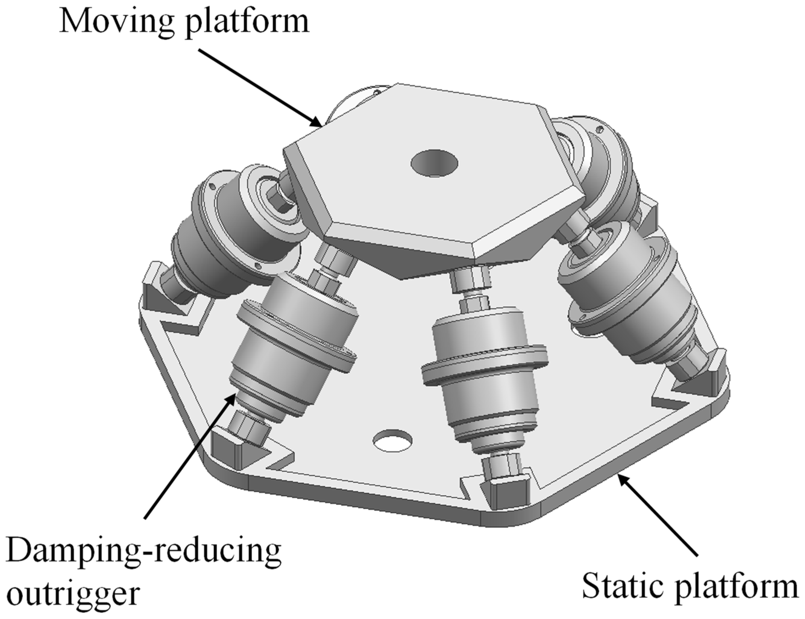
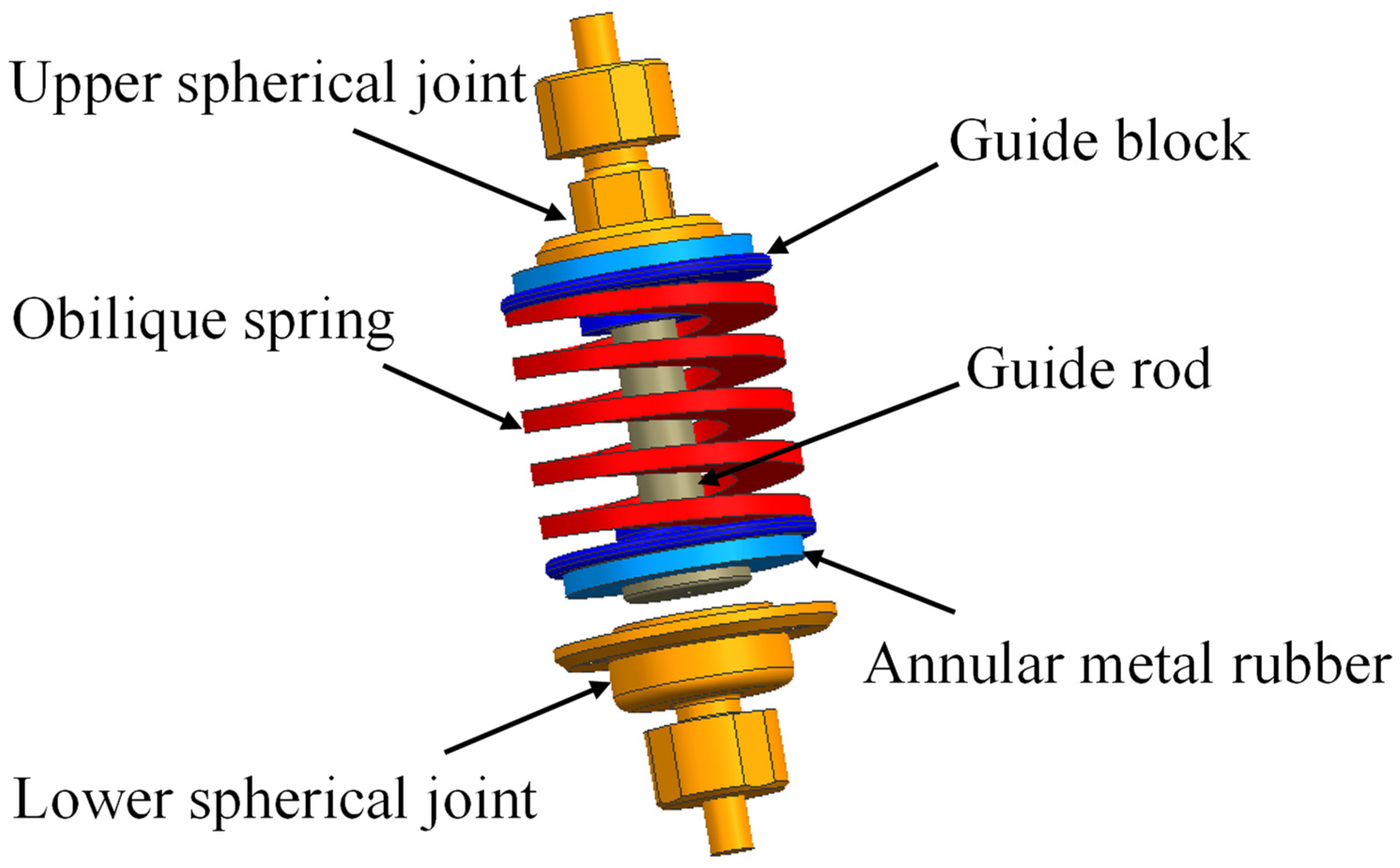
Aiming at the above problems and combining the characteristics of the Stewart platform, a 6-DOF all-metal vibration isolator, as shown in Figure 1, was designed in which the platform and the damping-reducing outrigger that is symmetrically distributed along the center axis are connected by spherical joints. It is a multi-free parallel vibration isolation system with the advantages of significant deformation, high temperature resistance, and shock resistance. Figure 2 illustrates the internal structure of the damping-reducing outrigger.

2.2. Structural Simplification

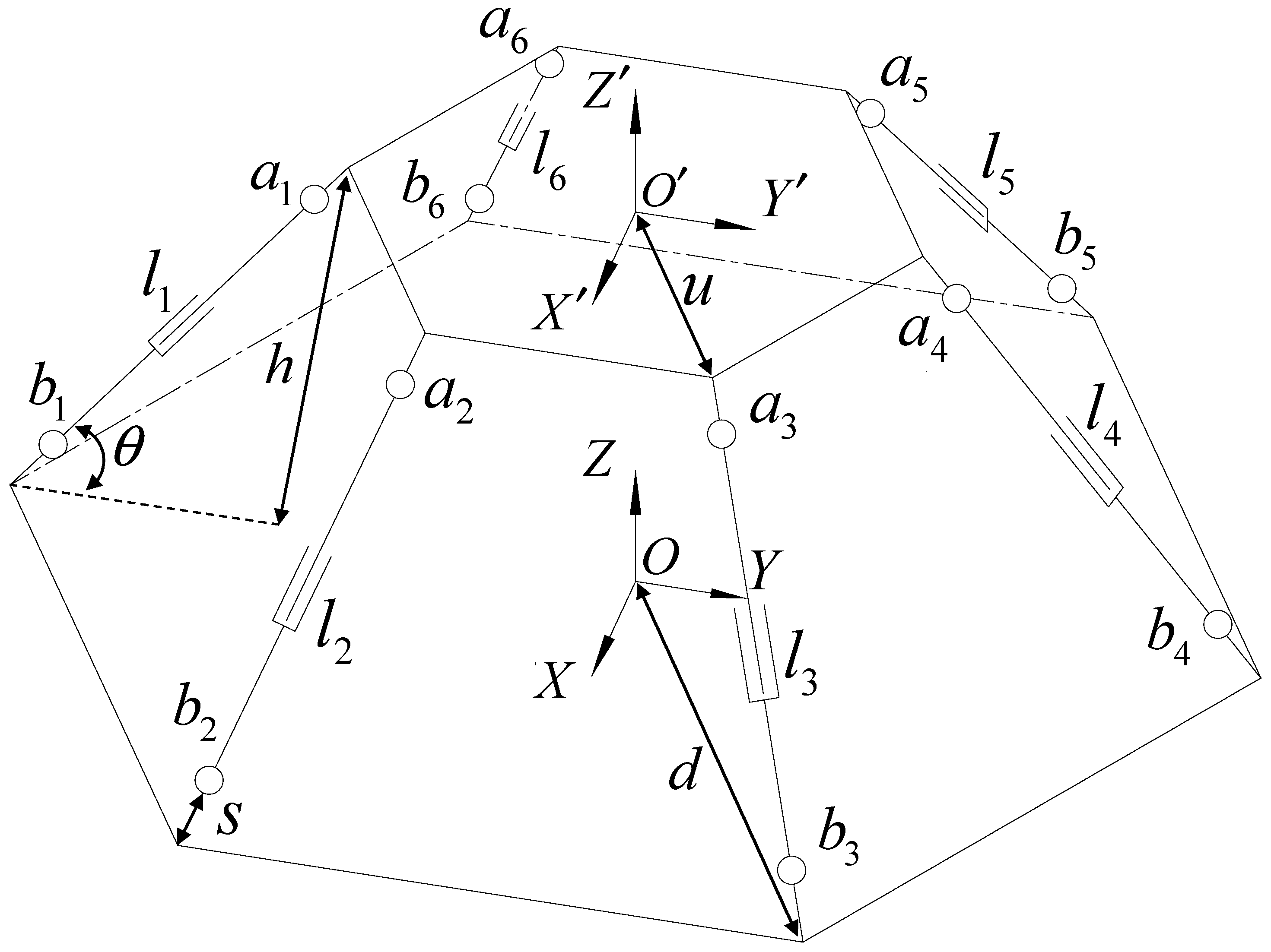
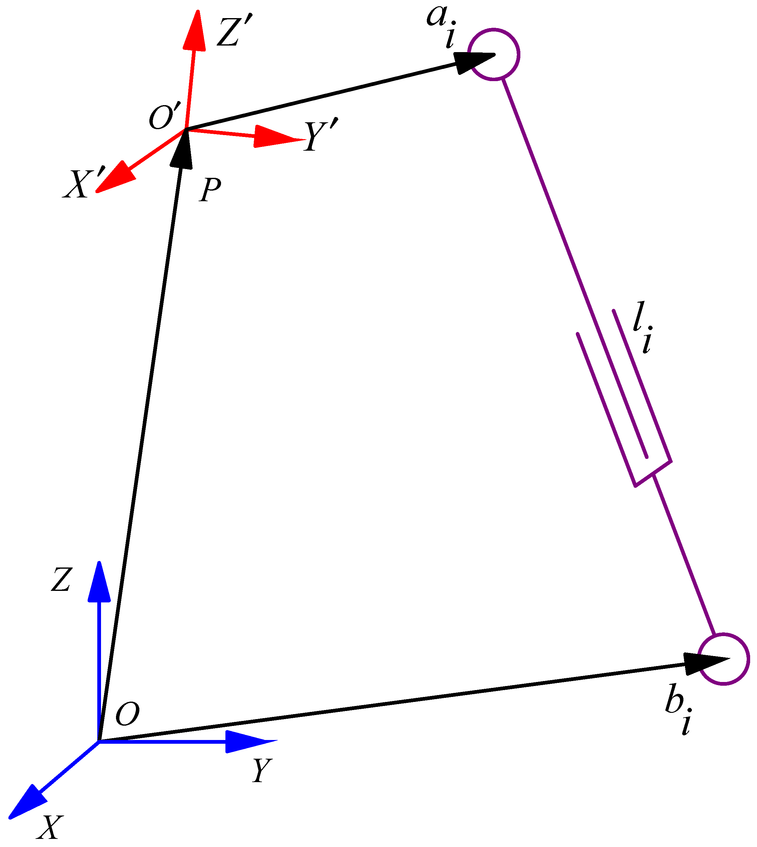
Figure 3 is the simplified structure diagram of the proposed 6-DOF all-metal vibration isolator. The moving and static coordinate systems ($O^{\prime }-X^{\prime }{Y}^{\prime }{Z}^{\prime }$ and $O-XYZ$) are established on the moving and static platforms. u and d represent the distance between the coordinate centers and boundaries for moving and static platforms, respectively. h is the height of the 6-DOF vibration isolator, respectively. s is the distance between the platform and the center of spherical joint, respectively. θ and l_i $(i=1,2,\cdots ,6)$ stand for the angle and the initial length of the damping-reducing outrigger. Therefore, all l_i $(i=1,2,\cdots ,6)$ can be expressed by $\mathit{h}/\cos \mathit{\theta }-2\mathit{s}$. The coordinate values of all spherical joints in the moving and static coordinate systems are, respectively:

$$\{\begin{array}{l}{\mathit{a}}_1={[0,-(\mathit{u}+\mathit{s}\cos \mathit{\theta }),-\mathit{s}\sin \mathit{\theta }]}^{\mathrm{T}}\\ {\mathit{a}}_2={[\frac{\sqrt{3}}{2}(\mathit{u}+\mathit{s}\cos \mathit{\theta }),-\frac{1}{2}(\mathit{u}+\mathit{s}\cos \mathit{\theta }),-\mathit{s}\sin \mathit{\theta }]}^{\mathrm{T}}\\ {\mathit{a}}_3={[\frac{\sqrt{3}}{2}(\mathit{u}+\mathit{s}\cos \mathit{\theta }),\frac{1}{2}(\mathit{u}+\mathit{s}\cos \mathit{\theta }),-\mathit{s}\sin \mathit{\theta }]}^{\mathrm{T}}\\ {\mathit{a}}_4={[0,\mathit{u}+\mathit{s}\cos \mathit{\theta },-\mathit{s}\sin \mathit{\theta }]}^{\mathrm{T}}\\ {\mathit{a}}_5={[-\frac{\sqrt{3}}{2}(\mathit{u}+\mathit{s}\cos \mathit{\theta }),\frac{1}{2}(\mathit{u}+\mathit{s}\cos \mathit{\theta }),-\mathit{s}\sin \mathit{\theta }]}^{\mathrm{T}}\\ {\mathit{a}}_6={[-\frac{\sqrt{3}}{2}(\mathit{u}+\mathit{s}\cos \mathit{\theta }),-\frac{1}{2}(\mathit{u}+\mathit{s}\cos \mathit{\theta }),-\mathit{s}\sin \mathit{\theta }]}^{\mathrm{T}}\end{array},\{\begin{array}{l}{\mathit{b}}_1={[0,-(\mathit{d}-\mathit{s}\cos \mathit{\theta }),\mathit{s}\sin \mathit{\theta }]}^{\mathrm{T}}\\ {\mathit{b}}_2={[\frac{\sqrt{3}}{2}(\mathit{d}-\mathit{s}\cos \mathit{\theta }),-\frac{1}{2}(\mathit{d}-\mathit{s}\cos \mathit{\theta }),\mathit{s}\sin \mathit{\theta }]}^{\mathrm{T}}\\ {\mathit{b}}_3={[\frac{\sqrt{3}}{2}(\mathit{d}-\mathit{s}\cos \mathit{\theta }),\frac{1}{2}(\mathit{d}-\mathit{s}\cos \mathit{\theta }),\mathit{s}\sin \mathit{\theta }]}^{\mathrm{T}}\\ {\mathit{b}}_4={[0,\mathit{d}-\mathit{s}\cos \mathit{\theta },\mathit{s}\sin \mathit{\theta }]}^{\mathrm{T}}\\ {\mathit{b}}_5={[-\frac{\sqrt{3}}{2}(\mathit{d}-\mathit{s}\cos \mathit{\theta }),\frac{1}{2}(\mathit{d}-\mathit{s}\cos \mathit{\theta }),\mathit{s}\sin \mathit{\theta }]}^{\mathrm{T}}\\ {\mathit{b}}_6={[-\frac{\sqrt{3}}{2}(\mathit{d}-\mathit{s}\cos \mathit{\theta }),-\frac{1}{2}(\mathit{d}-\mathit{s}\cos \mathit{\theta }),\mathit{s}\sin \mathit{\theta }]}^{\mathrm{T}}\end{array}$$

3. Forward Kinematic Algorithm of 6-DOF All-Metal Vibration Isolator

3.1. Quaternion and Dual Quaternion

Hamilton quaternion H is expressed as $\mathit{q}=q_{1}i+q_{2}j+q_{3}k+q_0$ or $\mathit{q}=(q,q_0)$, with the special rule that $q=Jm(\mathit{q})$, $q_0=Re(\mathit{q})$, $q_1,q_2,q_3,q_0\in R$, $i^2=j^2=k^2=-1$, $ij=-ji=k$, $jk=-kj=i$ and $ki=-ik=j$. The multiplication of two quaternions is still a quaternion, as:

$$(\mathit{q},\mathit{p})\to \mathit{q}\mathit{p}=\{q_{0}p+p_{0}q+q\times p,q_0{p}_0-q\cdot p\}$$

(1)

where $\mathit{p}=p_{1}i+p_{2}j+p_{3}k+p_0$, $\mathit{p}\in H$.

Similarly, the addition and subtraction of two quaternions result in quaternions, as:

$$(q,q_0)\pm (p,p_0)=(q\pm p,q_0\pm p_0)$$

(2)

In addition, a quaternion has the following properties:

$${\mathit{q}}^{*}=(-q,q_0),\Vert \mathit{q}\Vert =\sqrt{q_1{}^2+q_2{}^2+q_3{}^2+q_0{}^2},\mathrm{and}{\mathit{q}}^{-1}=\frac{{\mathit{q}}^{\ast }}{{\Vert \mathit{q}\Vert }^2}$$

(3)

$\Vert \mathit{q}\Vert =\sqrt{q_1{}^2+q_2{}^2+q_3{}^2+q_0{}^2}=1$ is defined as a unit quaternion, which has the following properties:

$$\mathit{q}{\mathit{q}}^{\ast }={\mathit{q}}^{\ast }\mathit{q}=1,\mathrm{and}{\mathit{q}}^{-1}={\mathit{q}}^{\ast }$$

(4)

Clifford dual quaternion $H\otimes D$ is expressed as $\widehat{\mathit{u}}={\mathit{q}}_r+{\mathit{q}}_d\mathit{\epsilon }$ or $\widehat{\mathit{u}}=[{\mathit{q}}_r,{\mathit{q}}_d]$, $\widehat{\mathit{u}}\in H\otimes D$, ${\mathit{q}}_r\in H$, ${\mathit{q}}_d\in H$ where ${\mathit{q}}_r$ and ${\mathit{q}}_d$ are the original part and dual part, respectively. $\mathit{\epsilon }$ is the dual calculation symbol, and ${\mathit{\epsilon }}^2=0$.

The multiplication of two dual quaternions is still a dual quaternion, as:

$${\widehat{\mathit{u}}}_1{\widehat{\mathit{u}}}_2=[{\mathit{q}}_r{}_1,{\mathit{q}}_d{}_1][{\mathit{q}}_r{}_2,{\mathit{q}}_d{}_2]=[{\mathit{q}}_r{}_1{\mathit{q}}_r{}_2,{\mathit{q}}_r{}_1{\mathit{q}}_d{}_2+{\mathit{q}}_d{}_1{\mathit{q}}_r{}_2],{\mathit{q}}_r{}_1\in H,{\mathit{q}}_d{}_1\in H,{\mathit{q}}_r{}_2\in H,{\mathit{q}}_d{}_2\in H$$

(5)

Similarly, the addition and subtraction of two dual quaternions result in dual quaternions, as:

$${\widehat{\mathit{u}}}_1\pm {\widehat{\mathit{u}}}_2=[{\mathit{q}}_r{}_1,{\mathit{q}}_d{}_1]\pm [{\mathit{q}}_r{}_2,{\mathit{q}}_d{}_2]=[{\mathit{q}}_r{}_1\pm {\mathit{q}}_r{}_2,{\mathit{q}}_d{}_1\pm {\mathit{q}}_d{}_2]$$

(6)

The dual quaternion $\overline{\widehat{\mathit{u}}}=[{\mathit{q}}_r,-{\mathit{q}}_d]$ is called the conjugate of dual, which is based on the definition of the dual conjugate. The dual quaternion ${\widehat{\mathit{u}}}^{\ast }=[{\mathit{q}}_r{}^{\ast },{\mathit{q}}_d{}^{\ast }]$ is called the conjugate of the dual quaternion, which is based on the definition of the dual quaternion conjugate. Combining the above two conjugate definitions, the compound conjugate definition of dual quaternion is expressed as:

$$\overline{{\widehat{\mathit{u}}}^{\ast }}={\overline{\widehat{\mathit{u}}}}^{\ast }=[{\mathit{q}}_r{}^{\ast },-{\mathit{q}}_d{}^{\ast }]$$

(7)

In addition, the conjugate of the dual quaternion has the following properties:

$${({\widehat{\mathit{u}}}_1{\widehat{\mathit{u}}}_2)}^{\ast }={\widehat{\mathit{u}}}_2{}^{\ast }{\widehat{\mathit{u}}}_1{}^{\ast },(\overline{{\widehat{\mathit{u}}}_1{\widehat{\mathit{u}}}_2})={\overline{\widehat{\mathit{u}}}}_1{\overline{\widehat{\mathit{u}}}}_2$$

(8)

Unlike quaternions, the norm of dual quaternions is even:

$$\Vert \widehat{\mathit{u}}\Vert =[\Vert {\mathit{q}}_r\Vert ,\frac{{\mathit{q}}_d{\mathit{q}}_r{}^{\ast }+{\mathit{q}}_r{\mathit{q}}_d{}^{\ast }}{2\Vert {\mathit{q}}_r\Vert }]$$

(9)

Similarly to quaternions, the inverse and norm multiplication of dual quaternions have the following properties:

$${\widehat{\mathit{u}}}^{-1}=\frac{{\widehat{\mathit{u}}}^{\ast }}{{\Vert \widehat{\mathit{u}}\Vert }^2},\Vert {\widehat{\mathit{u}}}_1{\widehat{\mathit{u}}}_2\Vert =\Vert {\widehat{\mathit{u}}}_1\Vert \Vert {\widehat{\mathit{u}}}_2\Vert$$

(10)

$\Vert \widehat{\mathit{u}}\Vert =1$ is defined as a unit dual quaternion, which has the following properties:

$$\Vert {\mathit{q}}_r\Vert =1,{\mathit{q}}_d{\mathit{q}}_r{}^{\ast }+{\mathit{q}}_r{\mathit{q}}_d{}^{\ast }=0$$

(11)

Further, the inverse of the unit dual quaternion is equal to the conjugate:

$${\widehat{\mathit{u}}}^{-1}={\widehat{\mathit{u}}}^{\ast }$$

(12)

The dual quaternion ${\widehat{\mathit{u}}}_{\mathit{q}}=[q,0]$ and the quaternion ${\mathit{v}}_0=[x_r,y_r,z_r,0]$ are extended by unit quaternion q and rotation vector $(x_r,y_r,z_r)$. Further, ${\mathit{v}}_0$ is expanded into a dual quaternion $\widehat{v}=[1,v_0]$. The rotation can be expressed as:

$$\widehat{v^{\prime }}={\widehat{\mathit{u}}}_q\widehat{v}{\overline{\widehat{\mathit{u}}}}_q^{\ast }=[\mathit{q},0][1,v_0][{\mathit{q}}^{\ast },0]=[\mathit{q},0][1,v_0]{[\overline{\mathit{q},0}]}^{\ast }=[1,{v^{\prime }}_0]$$

(13)

From Equation (13), the unit dual quaternion ${\widehat{\mathit{u}}}_q$ represents a pure rotation.

Similarly, the quaternion $\mathit{t}=[x_d,y_d,z_d,0]$ and the dual quaternion ${\widehat{\mathit{u}}}_t=[1,0.5\mathit{t}]$ are extended by displacement vector $(x_d,y_d,z_d)$. The displacement can be expressed as:

$$\widehat{v_{‵}}={\widehat{\mathit{u}}}_t\widehat{v}{\overline{\widehat{\mathit{u}}}}_t^{*}=[1,0.5\mathit{t}][1,v_0][1,0.5\mathit{t}]=[1,0.5\mathit{t}][1,v_0]{[\overline{1,0.5\mathit{t}}]}^{\ast }=[1,v_0+\mathit{t}]$$

(14)

From Equation (14), the unit dual quaternion ${\widehat{u}}_t$ represent a pure displacement.

Next, the rotation plus displacement can then be expressed as:

$$‘\widehat{v^{\prime }}={\widehat{\mathit{u}}}_t\left({\widehat{\mathit{u}}}_q\widehat{v}{\overline{\widehat{\mathit{u}}}}_q^{*}\right){\overline{\widehat{\mathit{u}}}}_t^{*}=({\widehat{\mathit{u}}}_t{\widehat{\mathit{u}}}_q)\widehat{v}({\overline{\widehat{\mathit{u}}}}_q^{\ast }{\overline{\widehat{\mathit{u}}}}_t^{\ast })=({\widehat{\mathit{u}}}_t{\widehat{\mathit{u}}}_q)\widehat{v}{(\overline{{\widehat{\mathit{u}}}_t{\widehat{\mathit{u}}}_q})}^{\ast }$$

(15)

${\widehat{\mathit{u}}}_{tq}={\widehat{\mathit{u}}}_t{\widehat{\mathit{u}}}_q=[1,0.5\mathit{t}][\mathit{q},0]=[\mathit{q},0.5\mathit{t}\mathit{q}]$ is defined; thus, ${\overline{\widehat{\mathit{u}}}}^{\ast }{}_{tq}={[\overline{\mathit{q},0.5\mathit{t}\mathit{q}}]}^{\ast }=[{\mathit{q}}^{\ast },-0.5{\left(\mathit{t}\mathit{q}\right)}^{\ast }]$.

Then, $‘\widehat{v^{\prime }}=({\widehat{\mathit{u}}}_{tq})\widehat{v}{({\overline{\widehat{\mathit{u}}}}_{tq})}^{\ast }=[\mathit{q},0.5\mathit{t}\mathit{q}][1,v_0][{\mathit{q}}^{\ast },-0,5{(\mathit{t}\mathit{q})}^{\ast }]=[1,\mathit{t}+\mathit{q}{v}_0{\mathit{q}}^{\ast }]$.

Under the properties of the dual quaternion norm, $\Vert {\widehat{u}}_{tq}\Vert =\Vert {\widehat{\mathit{u}}}_t\Vert \Vert {\widehat{\mathit{u}}}_q\Vert =1$ is still a unit dual quaternion, which means that any unit dual quaternion can represent rotation plus displacement.

3.2. Rigid Body Pose Calculation through Unit Dual Quaternion

Many methods have been used to describe the pose of a rigid body, and the most popular one is a 4 × 4 homogeneous transformation matrix, as given below.

$$T=\left[\begin{array}{cc}\mathit{R}& \mathit{P}\\ 0& 1\end{array}\right],\mathit{P}=\left[\begin{array}{c}{P}_x\\ P_y\\ P_z\end{array}\right]$$

(16)

$$\mathit{R}=Euler(\alpha ,\beta ,\gamma )=\left[\begin{array}{ccc}\cos \beta \cos \gamma & \sin \alpha \sin \beta \cos \gamma -\cos \alpha \sin \gamma & \cos \alpha \sin \beta \cos \gamma +\sin \alpha \sin \gamma \\ \cos \beta \sin \gamma & \cos \alpha \cos \gamma +\sin \alpha \sin \beta \sin \gamma & -\sin \alpha \cos \gamma +\cos \alpha \sin \beta \sin \gamma \\ -\sin \beta & \sin \alpha \cos \beta & \cos \alpha \cos \beta \end{array}\right]$$

(17)

where P stands for the absolute position and R for the orientation of the moving coordinate system.

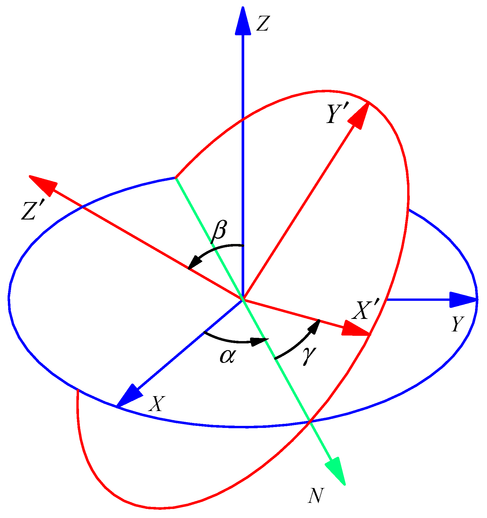
Figure 4 shows Euler angle conversion between moving and static coordinates: ($O^{\prime }-X^{\prime }{Y}^{\prime }{Z}^{\prime }$ and $O-XYZ$), where the intersection of the $XY$-plane and the $X^{\prime }{Y}^{\prime }$-plane is the line of intersection, represented by the letter $N$. $\alpha$ is the angle between the $X$-axis and the intersecting line; $\beta$ is the angle between the $Z$-axis and the $Z^{\prime }$-axis; and $\gamma$ is the angle between the intersecting line and the $X^{\prime }$-axis. and $O-XYZ$).

For forward kinematics, the length of the outrigger is given $l_i(i=1,2,\cdots ,6)$, and the position and orientation parameters ($P$ and $R$) of the moving platform are solved. The forward kinematics equation of the 6-DOF vibration isolator is shown:

$$E({\mathit{l}}_i)=\mathit{P}+\mathit{R}{\mathit{a}}_i,(i=1,2,\cdots ,6)$$

(18)

where ${\mathit{a}}_i$ represents the position vector of each branch chain in the moving coordinate system.

Unit quaternions $\mathit{q}$ often represent the rotation of a rigid body instead of the rotation matrix $\mathit{R}$, and satisfy the following equation:

$$\mathit{E}({\mathit{l}}_i)=\mathit{P}+\mathit{R}{\mathit{a}}_i=\mathit{P}+\mathit{q}{\mathit{a}}_i{\mathit{q}}^{\ast },(i=1,2,\cdots ,6)$$

(19)

The relationship between the dual quaternion and the homogeneous transfer matrix can be expressed as follows:

$$\mathit{R}=\left[\begin{array}{ccc}2q_0{}^2+2q_1{}^2-1& 2q_1{q}_2-2q_0{q}_3& 2q_1{q}_3+2q_0{q}_2\\ 2q_1{q}_2+2q_0{q}_3& 2q_0{}^2+2q_2{}^2-1& 2q_2{q}_3-2q_0{q}_1\\ 2q_1{q}_3-2q_0{q}_2& 2q_2{q}_3+2q_0{q}_1& 2q_0{}^2+2q_3{}^2-1\end{array}\right]$$

(20)

In Equation (19), the unit quaternion only represents rotation, not displacement. Through the deduction of Equation (14), the unit dual quaternion $\widehat{\mathit{u}}=[{\mathit{q}}_r,{\mathit{q}}_d]$ represents the position vector of each branch link connection point in the static coordinate system ($O-XYZ$ in Figure 3). First, ${\mathit{a}}_i=(a_{ix},a_{iy},a_{iz})$, $(i=1,2,\cdots ,6)$ is extended to quaternion form ${\mathit{a}}_{qi}=[{\mathit{a}}_i,0]$, and then to dual quaternion $[1,{\mathit{a}}_{qi}]$. In the same way, $E({\mathit{l}}_i)$ is extended to quaternion $E^q({\mathit{l}}_i)=[E\left({\mathit{l}}_i\right),0]$ and dual quaternion $[1,{\mathit{E}}^q({\mathit{l}}_i)]$. Therefore, Equation (19) can be expressed as:

$$[1,{\mathit{E}}^q({\mathit{l}}_i)]=\widehat{\mathit{u}}[1,{\mathit{a}}_{qi}]{\overline{\widehat{\mathit{u}}}}^{\ast }=[{\mathit{q}}_r,{\mathit{q}}_d][1,{\mathit{a}}_{\mathit{q}i}][{\mathit{q}}_r{}^{\ast },-{\mathit{q}}_d{}^{\ast }]=[1,2Jm({\mathit{q}}_d{\mathit{q}}_r{}^{\ast })+{\mathit{q}}_r{\mathit{a}}_{qi}{\mathit{q}}_r{}^{\ast }]$$

(21)

3.3. Forward Kinematics Equations

Based on Equation (21), the rotation and movement of the moving platform are transformed into quaternions by dual quaternion transformation. The closed-loop relationship between the outrigger vectors is shown in Figure 5.

Further, the close-loop kinematic equations are established as:

$${\mathit{l}}_i{\mathit{e}}_i+{\mathit{b}}_i=\mathit{P}+\mathit{R}{\mathit{a}}_i,(i=1,2,\cdots ,6)$$

(22)

where ${\mathit{b}}_i=(b_{ix},b_{iy},b_{iz})$ represents the position vector of each branch chain in the static coordinate system and ${\mathit{l}}_i$ represents the length of each damping-reducing outrigger. Further, the closed-loop equation is extended to quaternion form, and the closed-loop equation for all quaternions can be obtained by combining Equations (21) and (22):

$${\mathit{l}}_i[{\mathit{e}}_i,0]=[2Jm({\mathit{q}}_d{\mathit{q}}_r{}^{*}),0]+{\mathit{q}}_r[{\mathit{a}}_i,0]{\mathit{q}}_r{}^{*}-[{\mathit{b}}_i,0],(i=1,2,\cdots ,6)$$

(23)

The unit dual quaternion property, $\Vert \widehat{\mathit{u}}\Vert =1$, drew the following conclusion:

$$\{\begin{array}{l}\Vert {\mathit{q}}_r\Vert =1\\ {\mathit{q}}_d{\mathit{q}}_r{}^{\ast }+{\mathit{q}}_r{\mathit{q}}_d{}^{\ast }=Re({\mathit{q}}_d{\mathit{q}}_r{}^{\ast })=0\end{array}$$

(24)

Further, the kinematic closed-loop equation is simplified as:

$${\mathit{l}}_i[{\mathit{e}}_i,0]=2[{\mathit{q}}_d{\mathit{q}}_r{}^{*}-\mathrm{Re}({\mathit{q}}_d{\mathit{q}}_r{}^{*})]+{\mathit{q}}_r[{\mathit{a}}_i,0]{\mathit{q}}_r{}^{*}-[{\mathit{b}}_i,0]=2{\mathit{q}}_d{\mathit{q}}_r{}^{*}+{\mathit{q}}_r[{\mathit{a}}_i,0]{\mathit{q}}_r{}^{*}-[{\mathit{b}}_i,0]$$

(25)

Through the above transformation, the problem of solving the position and orientation is converted into the problem of solving quaternions ${\mathit{q}}_d$ and ${\mathit{q}}_r$. To reduce the power of ${\mathit{q}}_r$ and reduce the difficulty of the solution, ${\mathit{q}}_r$ is multiplied on both sides of Equation (25). The inner product of Equation (25) is further solved, and then the damping-reducing outrigger length equation can be obtained as:

$$\begin{array}{l}{\Vert {\mathit{l}}_i\Vert }^2=4{\Vert {\mathit{q}}_d\Vert }^2+{\Vert {\mathit{a}}_i\Vert }^2+{\Vert {\mathit{b}}_i\Vert }^2+4{\mathit{q}}_d\times {\mathit{q}}_r[{\mathit{a}}_i,0]-4{\mathit{q}}_d\times [{\mathit{b}}_i,0]{\mathit{q}}_r-2{\mathit{q}}_r[{\mathit{a}}_i,0]\times [{\mathit{b}}_i,0]{\mathit{q}}_r\\ (\mathit{i}=1,2,\cdot \cdot \cdot ,6)\end{array}$$

(26)

In Equation (26), the highest power of ${\mathit{q}}_d$ and ${\mathit{q}}_r$ is not more than two, so it can be written in the quadratic form by $\mathit{x}$:

$${\mathit{f}}_i(\mathit{x})=\frac{1}{2}{\mathit{x}}^{\mathrm{T}}{\mathit{Q}}_i\mathit{x}+{\mathit{C}}_i=0,(i=1,2,\cdots ,6)$$

(27)

where ${\mathit{C}}_i={\Vert {\mathit{a}}_i\Vert }^2+{\Vert {\mathit{b}}_i\Vert }^2-{\Vert {\mathit{l}}_i\Vert }^2$, $\mathit{x}={(q_{r1},q_{r2},q_{r3},q_{r0},q_{d1},q_{d2},q_{d3},q_{d0})}^{\mathrm{T}}$.

${\mathit{Q}}_i$ can be expressed in the form of a component block matrix, as:

$${\mathit{Q}}_i=\left[\begin{array}{cc}{\mathit{Q}}_{i11}& {\mathit{Q}}_{i12}\\ {\mathit{Q}}_{i21}& {\mathit{Q}}_{i22}\end{array}\right]$$

(28)

where ${\mathit{Q}}_{i11}=8{\mathit{E}}^{4\times 4}$, ${\mathit{Q}}_{i12}={\mathit{Q}}_{i21}{}^{\mathrm{T}}$. ${\mathit{Q}}_{i12}$ and ${\mathit{Q}}_{i21}$ are antisymmetric matrices. ${\mathit{Q}}_{i22}$ is a symmetric matrix, and each block matrix is listed as follows:

$${\mathit{Q}}_{i12}={\mathit{Q}}_{i21}^{\mathrm{T}}=\left[\begin{array}{cccc}0& 4{\mathit{A}}_{iz}& -4{\mathit{A}}_{iy}& 4{\mathit{B}}_{ix}\\ -4{\mathit{A}}_{iz}& 0& 4{\mathit{A}}_{ix}& 4{\mathit{B}}_{iy}\\ 4{\mathit{A}}_{iy}& -4{\mathit{A}}_{ix}& 0& 4{\mathit{B}}_{iz}\\ -4{\mathit{B}}_{ix}& -4{\mathit{B}}_{iy}& -4{\mathit{B}}_{iz}& 0\end{array}\right]$$

(29)

$${\mathit{Q}}_{i22}=\left[\begin{array}{cccc}4{\mathit{a}}_i\cdot {\mathit{b}}_i-8a_{ix}{b}_{ix}& -4(a_{iy}{b}_{ix}+a{b}_{ix}{}_{iy})& -4(a_{iz}{b}_{ix}+a_{ix}{b}_{iz})& 4(a_{iz}{b}_{iy}-a_{iy}{b}_{iz})\\ -4(a_{iy}{b}_{ix}+a{b}_{ix}{}_{iy})& 4{\mathit{a}}_i\cdot {\mathit{b}}_i-8a_{iy}{b}_{iy}& -4(a_{iz}{b}_{iy}-a_{iy}{b}_{iz})& 4(a_{ix}{b}_{iz}-a_{iz}{b}_{ix})\\ -4(a_{iz}{b}_{ix}+a_{ix}{b}_{iz})& -4(a_{iz}{b}_{iy}-a_{iy}{b}_{iz})& 4{\mathit{a}}_i\cdot {\mathit{b}}_i-8a_{iz}{b}_{iz}& 4(a_{iy}{b}_{ix}-a_{ix}{b}_{iy})\\ 4(a_{iz}{b}_{iy}-a_{iy}{b}_{iz})& 4(a_{ix}{b}_{iz}-a_{iz}{b}_{ix})& 4(a_{iy}{b}_{ix}-a_{ix}{b}_{iy})& -4{\mathit{a}}_i\cdot {\mathit{b}}_i\end{array}\right]$$

(30)

where ${\mathit{A}}_i={\mathit{a}}_i+{\mathit{b}}_i$ and ${\mathit{B}}_i={\mathit{a}}_i-{\mathit{b}}_i$.

Similarly, Equation (24) is also converted into quadratic form, as:

$$\{\begin{array}{l}{f}_7(\mathit{x})=\frac{1}{2}{\mathit{x}}^{\mathrm{T}}{\mathit{Q}}_7\mathit{x}+C_7=0\\ f_8(\mathit{x})=\frac{1}{2}{\mathit{x}}^{\mathrm{T}}{\mathit{Q}}_8\mathit{x}+C_8=0\end{array},{\mathit{Q}}_7=\left[\begin{array}{cc}2{\mathrm{I}}^{4\times 4}& 0\\ 0& 0^{4\times 4}\end{array}\right],{\mathit{Q}}_8=\left[\begin{array}{cc}{0}^{4\times 4}& \mathrm{I}\\ \mathrm{I}& 0^{4\times 4}\end{array}\right],C_7=-1,C_8=0$$

(31)

3.4. Construction of an Iterative Sequence

Equations (27) and (31) are expressed in the form of nonlinear equations, as:

$$\mathit{f}(\mathit{x})=\frac{1}{2}{\mathit{x}}^{\mathrm{T}}\mathit{Q}\mathit{x}+\mathit{C}$$

(32)

where $\mathit{f}(\mathit{x})={(f_1(\mathit{x}),f_2(\mathit{x}),\cdots ,f_8(\mathit{x}))}^{\mathrm{T}},\mathit{Q}={({\mathit{Q}}_1,{\mathit{Q}}_2,\cdots ,{\mathit{Q}}_8)}^{\mathrm{T}}$, and $\mathit{C}={(C_1,C_2,\cdots ,C_8)}^{\mathrm{T}}$.

The $\mathit{f}(\mathit{x})$ is decomposed by the Taylor formula, and the higher-order term is ignored. Thus, the Newton–Raphson numerical iteration sequence can be obtained as:

$${\mathit{x}}_{k+1}={\mathit{x}}_k-{\mathit{J}}_x^q{}^{-1}\mathit{f}({\mathit{x}}_k),k=0,1,2\cdots$$

(33)

The greatest advantage of the Newton–Raphson method is fast convergence speed, but it is difficult to realize. The Newton–Raphson method is required to calculate the inverse matrix of the Jacobian matrix ${\mathit{J}}_x^q$ in each iteration, which increases the calculation amount.

The Broyden iterative method is introduced to reduce the amount of calculation. Replacing ${\mathit{J}}_x^q$ with matrix ${\mathit{A}}_k$ in a sense of approximation is essential for the Broyden iterative method. ${\mathit{A}}_k$ is nonsingular and easier to calculate than ${\mathit{J}}_x^q$. The general form of this iterative scheme is expressed as:

$$\{\begin{array}{l}{\mathit{A}}_k={\mathit{A}}_{k-1}+\frac{({\mathit{y}}_k-{\mathit{A}}_{k-1}{\mathit{s}}_k){\mathit{s}}_k^T}{{\mathit{s}}_k^T{\mathit{s}}_k}\\ {\mathit{x}}_{k+1}={\mathit{x}}_k-{\mathit{A}}_k{}^{-1}\mathit{f}({\mathit{x}}_k),k=1,2,3\cdots \end{array}$$

(34)

where ${\mathit{y}}_k=\mathit{f}({\mathit{x}}_k)-\mathit{f}({\mathit{x}}_{k-1})$, ${\mathit{s}}_k={\mathit{x}}_k-{\mathit{x}}_{k-1}$.

The relationship between the nonlinear equation group and the Jacobian matrix are obtained:

$${\mathit{J}}_x^q=\frac{\partial \mathit{f}({\mathit{x}}_k)}{\partial {\mathit{x}}_k}={\mathit{x}}_k{}^{\mathrm{T}}\mathit{Q}$$

(35)

$$\mathit{f}({\mathit{x}}_k)=\frac{1}{2}{\mathit{x}}_k^T\mathit{Q}{\mathit{x}}_k+\mathit{C}=\frac{1}{2}{\mathit{J}}_k{\mathit{x}}_k+\mathit{C}$$

(36)

Further, Equation (36) is substituted into Equation (34). Since $A_{\mathit{k}}\approx {\mathit{J}}_x^q$ is approximated in the Broyden iteration sequence, Equation (34) can be expressed as:

$$\{\begin{array}{l}{\mathit{A}}_k={\mathit{A}}_{k-1}+2{\mathit{A}}_{k-1}{\mathit{s}}_k{\mathit{s}}_k^{\mathrm{T}}{\mathit{U}}^{-1}\\ {\mathit{x}}_{k+1}=\frac{1}{2}{\mathit{x}}_k-{\mathit{A}}_k^{-1}\mathit{C},k=1,2,3\cdots \end{array}$$

(37)

where $\mathit{U}=-2{\mathit{s}}_k^{\mathrm{T}}{\mathit{s}}_k{\mathit{E}}_{8\times 8}+{\mathit{x}}_k{\mathit{s}}_k^{\mathrm{T}}$.

In Equation (37), the inverse matrix ${\mathit{A}}_k{}^{-1}$ needs to be solved during each iteration. Therefore, the matrix inversion formula of Sherman and Morrison is introduced:

$${(\mathit{A}+\mathit{x}{\mathit{y}}^{\mathrm{T}})}^{-1}={\mathit{A}}^{-1}-\frac{{\mathit{A}}^{-1}\mathit{x}{\mathit{y}}^{\mathrm{T}}{\mathit{A}}^{-1}}{1+{\mathit{y}}^{\mathrm{T}}{\mathit{A}}^{-1}\mathit{x}}$$

(38)

where $\Vert \mathit{A}\Vert \ne 0,{\mathit{y}}^{\mathrm{T}}{\mathit{A}}^{-1}\mathit{x}\ne -1$ and, thus, $\mathit{x}$ and $\mathit{y}$ are vectors.

Then, the $\mathit{A}={\mathit{A}}_{k-1},\mathit{x}={\mathit{A}}_{k-1}{\mathit{s}}_k,{\mathit{y}}^{\mathrm{T}}={\mathit{s}}_k^{\mathrm{T}}{\mathit{U}}^{-1}$ is substituted into Equation (38). Therefore, the iteration sequence is expressed as:

$$\{\begin{array}{l}{\mathit{A}}_k^{-1}={\mathit{A}}_{k-1}^{-1}-\frac{{\mathit{s}}_k{\mathit{s}}_k^{\mathrm{T}}{\mathit{U}}^{-1}{\mathit{A}}_{k-1}^{-1}}{1+s_k^{\mathrm{T}}{U}^{-1}{s}_k}\\ {\mathit{x}}_{k+1}=\frac{1}{2}{\mathit{x}}_k-{\mathit{A}}_k^{-1}\mathit{C},k=1,2,3\cdots \end{array}$$

(39)

After ${\mathit{A}}_0^{-1}={\left[{\mathit{f}}^{\prime }(x_0)\right]}^{-1}$ is solved, then ${\mathit{A}}_k^{-1}$ can be calculated by the recursive formula for each iteration step. However, the inverse matrix $\mathit{U}$ still exists in Equation (39). Therefore, Equation (38) is further applied to improve $\mathit{U}$. Then,$\mathit{A}=-2{\mathit{s}}_k^{\mathrm{T}}{\mathit{s}}_k{\mathit{E}}_{n\times n}$, $\mathit{x}={\mathit{x}}_k$,${\mathit{y}}^{\mathrm{T}}={\mathit{s}}_k^{\mathrm{T}}$ is substituted into Equation (38). Finally, the enhanced Broyden numerical iterative algorithm is obtained as:

$$\{\begin{array}{l}{\mathit{U}}^{-1}=-\frac{1}{2{\mathit{s}}_k^{\mathrm{T}}{\mathit{s}}_k}({\mathit{E}}_{8\times 8}+\frac{{\mathit{x}}_k{\mathit{s}}_k^{\mathrm{T}}}{{\mathit{s}}_k^{\mathrm{T}}({\mathit{x}}_k-2{\mathit{x}}_{k-1})})\\ {\mathit{A}}_k^{-1}={\mathit{A}}_{k-1}^{-1}-\frac{{\mathit{s}}_k{\mathit{s}}_k^{\mathrm{T}}{\mathit{U}}^{-1}{\mathit{A}}_{k-1}^{-1}}{1+{\mathit{s}}_k^{\mathrm{T}}{\mathit{U}}^{-1}{\mathit{s}}_k}\\ {\mathit{x}}_{k+1}=\frac{1}{2}{\mathit{x}}_k-{\mathit{A}}_k^{-1}\mathit{C},k=1,2,3\cdots \end{array}$$

(40)

The enhanced Broyden numerical iterative algorithm is no longer necessary to update the function value of $\mathit{f}(\mathit{x})$ and calculate any inverse matrix, which can greatly reduce the calculation difficulty. After the iteration converges, a unique set of variables ($q_{r1}$, $q_{r2}$, $q_{r3}$, $q_{r0}$, $q_{d1}$, $q_{d2}$, $q_{d3}$, $q_{d0}$) can be calculated, then the position vector and orientation matrix can be solved by Equations (20) and (24).

4. Numerical Solution

4.1. Determination of Dimension Parameters

Because of the particular structure of the vibration isolator, establishing the analytical model is very complicated. Thus, the linear assumption is adopted to guide the calculation of the approximate stiffness, and then the relevant parameters of the vibration isolator are determined. In addition, the load is assumed to be distributed symmetrically in the vertical direction of the isolator.

Based on the relationship between the load components, the stiffness of the vibration isolator in the vertical Z direction can be approximated as:

$$k_z=6k_n\sin \mathit{\theta }$$

(41)

The horizontal X-direction and Y-direction stiffness can be approximated as:

$$\begin{array}{l}{k}_x=4k_n\cos \mathit{\theta }\sin 60°=2\sqrt{3}{k}_n\cos \mathit{\theta }\\ k_y=2k_n\cos \mathit{\theta }+4k_n\cos \mathit{\theta }\cos 60°=4k_n\cos \mathit{\theta }\end{array}$$

(42)

The ratio of the horizontal stiffness to the vertical are obtained:

$$r_{k1}=\frac{k_x}{k_z}=\frac{\sqrt{3}}{3}\cot \mathit{\theta },r_{k2}=\frac{k_y}{k_z}=\frac{2}{3}\cot \mathit{\theta }$$

(43)

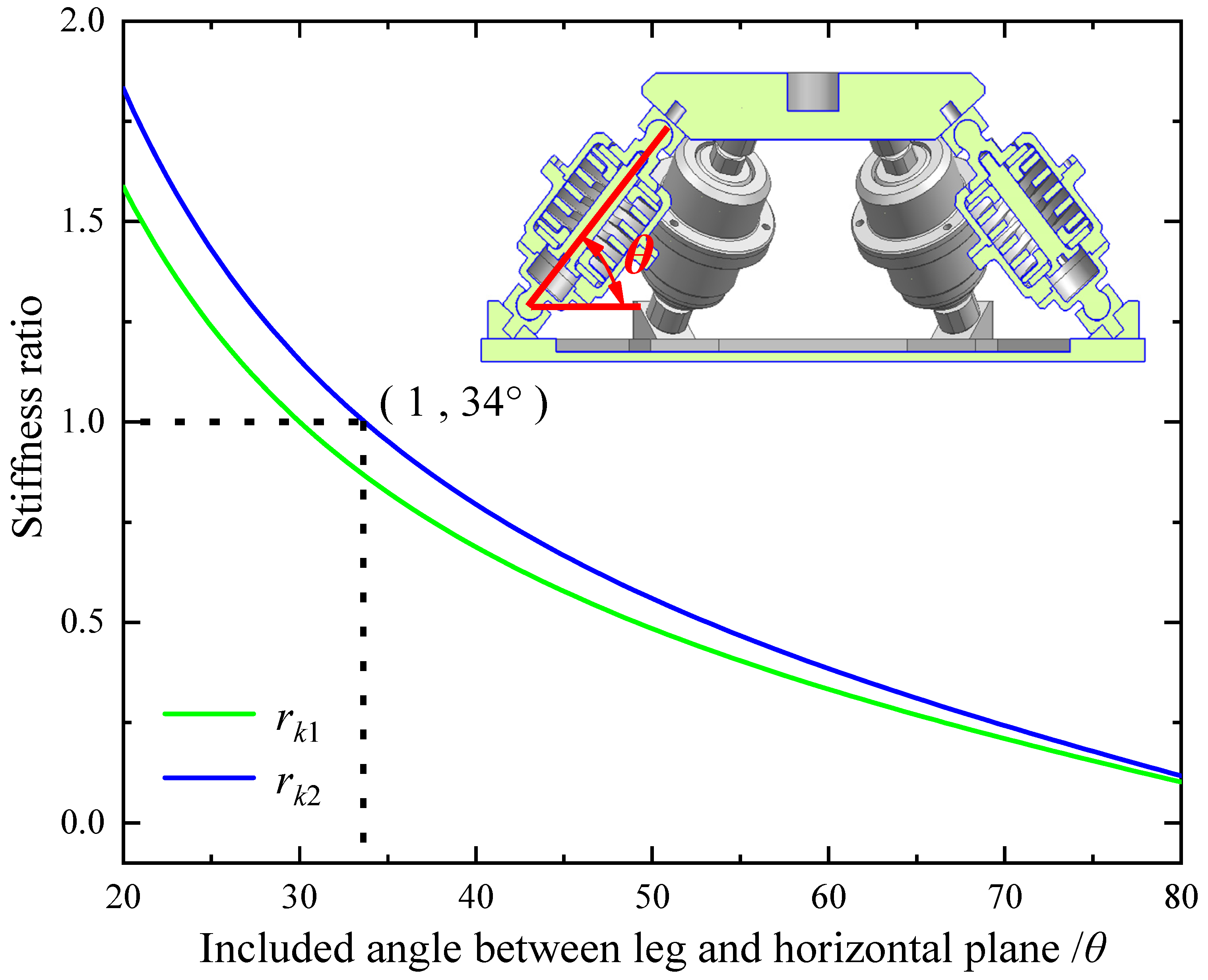
Figure 6 shows the approximate relationship curve between the ratio of vertical stiffness and the spatial inclination angle. It can be seen that the smaller the space angle between the damping-reducing outrigger and the horizontal plane, the greater the lateral stiffness, but the stiffness in the Z direction also decreases at this time. Since the magnitude of vibration from the horizontal direction is almost the same as that in the Z direction during operation, the three-dimensional stiffness should satisfy the following relationship:

$$k_z=\max (k_x,k_y)$$

(44)

Therefore, when $r_{k2}=1$, the space angle is $\mathit{\theta }\approx 34°$ between the damping-reducing outrigger and the horizontal plane.

The installation dimension requirements of the vibration isolator are: $\mathit{h}=100$, $\mathit{u}=77$, and $\mathit{d}=225$. In addition, for the model of the spherical joint, $\mathit{s}=9$. Therefore, the initial length ${\mathit{l}}_i=\mathit{h}/\cos \mathit{\theta }-2\mathit{s}\approx 160$, $(i=1,2,\cdots ,6)$, and the coordinate values of the upper spherical joint and the lower spherical joint can be obtained as follows:

$$\{\begin{array}{l}{\mathit{a}}_1={[0,-84.5,-5]}^{\mathrm{T}}\\ {\mathit{a}}_2={[73.2,-42.2,-5]}^{\mathrm{T}}\\ {\mathit{a}}_3={[73.2,42.2,-5]}^{\mathrm{T}}\\ {\mathit{a}}_4={[0,84.5,-5]}^{\mathrm{T}}\\ {\mathit{a}}_5={[-73.2,42.2,-5]}^{\mathrm{T}}\\ {\mathit{a}}_6={[-73.2,-42.2,-5]}^{\mathrm{T}}\end{array},\{\begin{array}{l}{\mathit{b}}_1={[0,-217.5,5]}^{\mathrm{T}}\\ {\mathit{b}}_2={[188.4,-108.8,5]}^{\mathrm{T}}\\ {\mathit{b}}_3={[188.4,108.8,5]}^{\mathrm{T}}\\ {\mathit{b}}_4={[0,217.5,5]}^{\mathrm{T}}\\ {\mathit{b}}_5={[-188.4,108.8,5]}^{\mathrm{T}}\\ {\mathit{b}}_6={[-188.4,-108.8,5]}^{\mathrm{T}}\end{array}$$

The damping-reducing outrigger stiffness is calculated as follows:

$$\frac{1}{k_d}=\frac{1}{k_s}+2\frac{1}{k_m}$$

(45)

where $k_d$ represents the damping-reducing outrigger stiffness; $k_s=337\mathrm{N}/\mathrm{mm}$ represents the oblique-springs stiffness; and $k_m=84\mathrm{N}/\mathrm{mm}$ represents the annular-shaped metal rubber stiffness. Based on Equations (45) and (42), the stiffness of the vibration isolator is 280 N/mm. Under the use requirements of the vibration isolator, the vibration isolator’s rated load is 2000 N. Therefore, the maximum static deformation is ±7.2 mm. According to the angle relationship, ${\mathit{l}}_i\approx 147.1~172.9\mathrm{mm}$, $(i=1,2,\cdots ,6)$. The load is fixedly connected with the vibration isolator through the moving platform (Figure 1). The load on the outrigger is greater than it is in the equilibrium state, when the load is torsional. Thus, the deformation range is estimated to be the minimum.

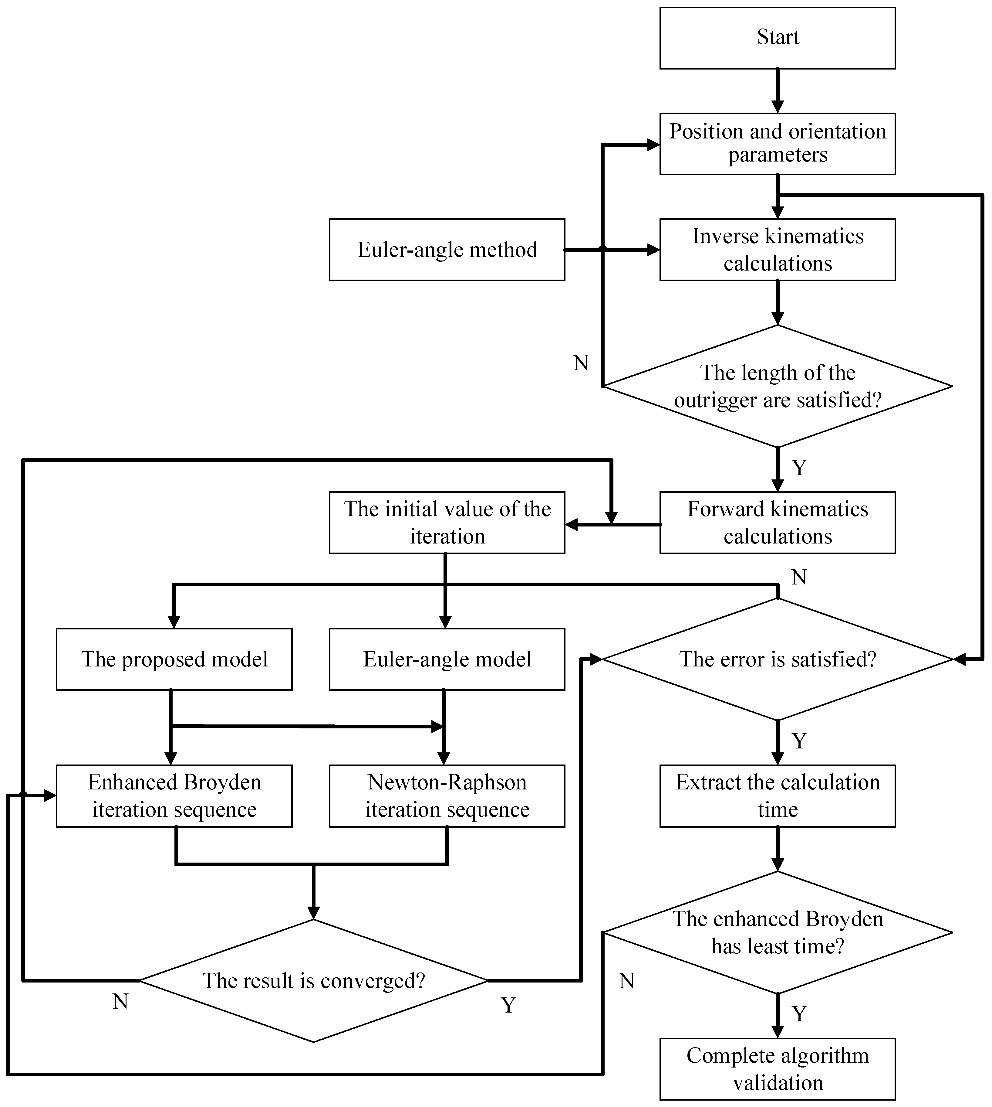
4.2. Simulation Methodology

Mathematica is an extremely powerful piece of software that not only provides a mathematical model of all the normal functions, but also performs deep calculations. Thus, the forward kinematics model of the 6-DOF isolator was solved iteratively by Mathematica, and its forward kinematics simulation method is shown in Figure 7.

4.3. Correctness Verification

The correctness verification of the algorithm includes the following two steps: first, the position and orientation of the 6-DOF isolator are given, and the length of each damping-reducing outrigger is calculated by using the calculation method of inverse kinematics. Further, taking the length of each damping-reducing outrigger as a condition, the forward kinematics algorithm is used to calculate the position and orientation. Finally, the calculation results are compared with the initial conditions.

The position vector $\mathit{P}=(5,15,100)$ and the orientation $\alpha =8°$, $\beta =-5°$, $\gamma =10°$ in the preset state are assumed. Then, the orientation matrix R is shaped as follows:

$$\mathit{R}=\left[\begin{array}{ccc}-0.23926011& -0.87431183& -0.42229541\\ -0.15685629& -0.39440993& 0.90544845\\ -0.9582018& 0.2828774& -0.04277475\end{array}\right]$$

Based on Equation (18), the relationship between the Euler angle and the damping-reducing outrigger length can be obtained as follows:

$${\Vert {\mathit{l}}_i\Vert }^2=(\mathit{P}+\mathit{R}{\mathit{a}}_i-{\mathit{b}}_i)\cdot (\mathit{P}+\mathit{R}{\mathit{a}}_i-{\mathit{b}}_i),(i=1,2,\cdots ,6)$$

(46)

Then, the length of the damping-reducing outrigger is calculated as:

$$l_1=171.418\mathrm{mm},l_2=167.8412\mathrm{mm},l_3=161.807\mathrm{mm},l_4=157.3133\mathrm{mm}{l}_5=158.8102\mathrm{mm},l_6=166.9887\mathrm{mm}$$

Figure 8 shows a schematic of the position and orientation of a 6-DOF all-metal vibration isolator. Based on Equations (20) and (24), the position and orientation of the moving platform are converted into parameters as:

$$\begin{gathered} {\mathit{q}}_r=(0.07454,-0.03229,0.1004,0.99141) \\ {\mathit{q}}_d=(4.61503,10.89008,48.36737,-4.9837) \end{gathered}$$

In addition, the length of each damping-reducing outrigger is within the range proposed above. Thus, the correctness of P and R is determined. The structural parameters and damping-reducing outrigger length are substituted into Equation (27) as:

$$\begin{array}{c}\mathit{C}={[25112.4,26350.4,28339.6,29749,29300.4,26635.9,-1,0]}^{\mathrm{T}}\hfill \\ {\mathit{Q}}_{112}={\mathit{Q}}_{121}^{\mathrm{T}}=\left[\begin{array}{cccc}0& 0& 1208& 0\\ 0& 0& 0& 532\\ -1208& 0& 0& -40\\ 0& -532& 40& 0\end{array}\right],{\mathit{Q}}_{122}=\left[\begin{array}{cccc}73415& 0& 0& 6040\\ 0& -73615& -2660& 0\\ 0& -2660& 73615& 0\\ 6040& 0& 0& -73415\end{array}\right]\hfill \\ {\mathit{Q}}_{212}={\mathit{Q}}_{221}^{\mathrm{T}}=\left[\begin{array}{cccc}0& 0& 604& -460.8\\ 0& 0& 1046.4& 266.4\\ -604& -1046.4& 0& -40\\ 460.8& -266.4& 40& 0\end{array}\right],{\mathit{Q}}_{222}=\left[\begin{array}{cccc}-36898.1& 63658.6& 2304& 3020\\ 63658.6& 36698.1& -1332& 5232\\ 2304& -1332& 73629& 54.8\\ 3020& 5232& 54.8& -73429\end{array}\right]\hfill \\ {\mathit{Q}}_{312}={\mathit{Q}}_{321}^{\mathrm{T}}=\left[\begin{array}{cccc}0& 0& -604& -460.8\\ 0& 0& 1046.4& -266.4\\ 604& -1046.4& 0& -40\\ 460.8& 266.4& 40& 0\end{array}\right],{\mathit{Q}}_{322}=\left[\begin{array}{cccc}-36898.1& -63658.6& 2304& -3020\\ -63658.6& 36698.1& 1332& 5232\\ 2304& 1332& 73629& -54.8\\ -3020& 5232& -54.8& -73429\end{array}\right]\hfill \\ {\mathit{Q}}_{412}={\mathit{Q}}_{421}^{\mathrm{T}}=\left[\begin{array}{cccc}0& 0& -1208& 0\\ 0& 0& 0& -532\\ 1208& 0& 0& -40\\ 0& 532& 40& 0\end{array}\right],{\mathit{Q}}_{422}=\left[\begin{array}{cccc}73415& 0& 0& -6040\\ 0& -73615& 2660& 0\\ 0& 2660& 73615& 0\\ -6040& 0& 0& -73415\end{array}\right]\hfill \\ {\mathit{Q}}_{512}={\mathit{Q}}_{521}^{\mathrm{T}}=\left[\begin{array}{cccc}0& 0& -604& 460.8\\ 0& 0& -1046.4& -266.4\\ 604& 1046.4& 0& -40\\ -460.8& 266.4& 40& 0\end{array}\right],{\mathit{Q}}_{522}=\left[\begin{array}{cccc}-36898.1& 63658.6& -2304& -3020\\ 63658.6& 36698.1& 1332& -5232\\ -2304& 1332& 73629& 54.8\\ -3020& -5232& 54.8& -73429\end{array}\right]\hfill \\ {\mathit{Q}}_{612}={\mathit{Q}}_{621}^{\mathrm{T}}=\left[\begin{array}{cccc}0& 0& 604& 460.8\\ 0& 0& -1046.4& 266.4\\ -604& 1046.4& 0& -40\\ -460.8& -266.4& 40& 0\end{array}\right],{\mathit{Q}}_{622}=\left[\begin{array}{cccc}-36898& -63658.6& -2304& 3020\\ -63658.6& 36698.1& -1332& -5232\\ -2304& -1332& 73629& -54.8\\ 3020& -5232& -54.8& -73429\end{array}\right]\hfill \end{array}$$

The initial posture ${\mathit{P}}_0=(9,4,90)$, ${\alpha }_0=11.5°$, ${\beta }_0=17°$, ${\gamma }_0=-11.5°$ is supposed and then converted into quaternion form as:

$$\begin{gathered} {\mathit{q}}_{r0}=(0.11218,0.1373,-0.12702,0.97591) \\ {\mathit{q}}_{d0}=(-0.94362,-6.171,33.87096,-5.38583) \end{gathered}$$

Given the accuracy $esp=0.0001$, the iterative process is shown in Figure 9. After fifteen iterations, the result is completely consistent with the inverse solution; then, the correctness of the algorithm is proven. In addition, the iteration time is 0.004 ms, and there are 19 iterative steps.

4.4. Efficiency Verification

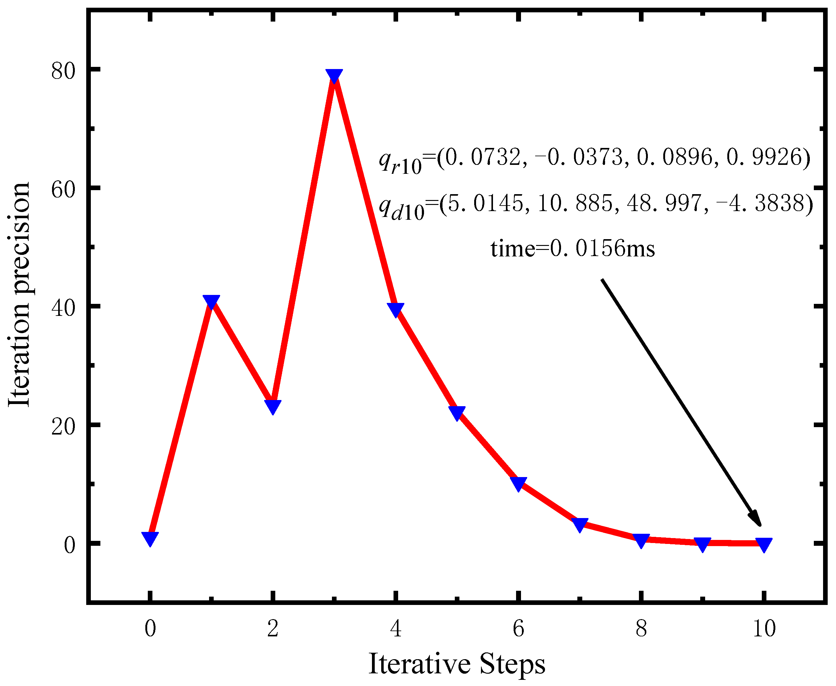
Using the same computer software, the efficiency is proven by comparing the results with those of the Newton–Raphson method described previously, using the traditional Euler angle and the dual quaternion. Figure 10 and Figure 11 show the iterative calculation results. There are 7 and 10 iterative steps, and the iterative times are 0.0312 ms and 0.0156. Compared with the traditional rotation-matrix method and the Newton–Raphson method, the computational efficiency of the enhanced Broyden numerical iterative algorithm is thus increased by 680% and 290%, respectively.

4.5. Discussion

The efficiency of the enhanced Broyden numerical iterative algorithm is very obvious, as can be seen from the results in Section 4.4. The main reason for this is that the enhanced Broyden numerical iterative algorithm does not need to calculate any inverse matrix and forward kinematics equations in the iterative process, which is untrue for the algorithms shown in Figure 10 and Figure 11. In addition, it can be seen that the calculation efficiency of the algorithm shown in Figure 10 is lower than that in Figure 11. The main reason is that the inverse matrix to be calculated in the algorithm shown in Figure 10 is an 8-order matrix, while that in Figure 11 is a 6-order matrix. The algorithms in Figure 10 and Figure 11 are based on the Newton–Raphson method, which has the property of square convergence. Thus, they use fewer iterative steps than the enhanced Broyden numerical iterative algorithm does, but the calculation time for each step is longer.

5. Singularity Analysis

5.1. Establishment of Kinematic Jacobian Matrix

The input–output kinematic equations of the vibration isolator based on the Jacobian matrix can be obtained by taking the derivative of Equation (18), which was concerned with time, as:

$${\mathit{J}}_x^q\dot{\mathit{x}}={\mathit{J}}_l^q\dot{\mathit{l}}$$

(47)

where

$$\begin{gathered} {\mathit{J}}_x^q=({\mathit{x}}^T{\mathit{Q}}_1,{\mathit{x}}^T{\mathit{Q}}_2,\cdots ,{\mathit{x}}^T{\mathit{Q}}_8),\dot{\mathit{x}}=({\dot{q}}_{r1},{\dot{q}}_{r2},{\dot{q}}_{r3},{\dot{q}}_{r0},{\dot{q}}_{d1},{\dot{q}}_{d2},{\dot{q}}_{d3},{\dot{q}}_{d0}), \\ {\mathit{J}}_l^q=2diag(l_1,l_2,l_3,l_4,l_5,l_6,0,0),\dot{\mathit{l}}=({\dot{l}}_1,{\dot{l}}_2,{\dot{l}}_3,{\dot{l}}_4,{\dot{l}}_5,{\dot{l}}_6,0,0) \end{gathered}$$

where ${\mathit{J}}_x^q$ is the forward kinematics Jacobian matrix and ${\mathit{J}}_l^q$ is the inverse kinematics Jacobian matrix. Obviously, $\det ({\mathit{J}}_l^q)\ne 0$; when $\det ({\mathit{J}}_x^q)=0$, the vibration isolator has forward kinematics singularity. Based on the forward kinematics algorithm, the singular trajectory of the isolator in the configuration space is a hypersurface distributed in the eight-dimensional parameter space. Therefore, to obtain the distribution law of singular trajectory conveniently, it is divided into two forms: position-singular configuration and orientation-singular configuration.

5.2. Position-Singularity Analysis

The position-singular configuration is located on $\mathit{R}\in \mathrm{SO}(4)$ when the orientation parameter ${\mathit{q}}_r$ is given. Since ${\mathit{q}}_d$ is not a unit quaternion, each element of ${\mathit{q}}_d$ has no value range. In addition, the imaginary part of $2{\mathit{q}}_d{\mathit{q}}_r{}^{\ast }$ represents the displacement, so conversion of ${\mathit{q}}_d$ into the expression of the spatial position parameter is necessary.

$$\{\begin{array}{l}{q}_{d0}=(q_{r1}{P}_x+q_{r2}{P}_y+q_{r3}{P}_z)/2\\ q_{d1}=(-q_{r0}{P}_x-q_{r3}{P}_y+q_{r2}{P}_z)/2\\ q_{d2}=(q_{r3}{P}_x-q_{r0}{P}_y-q_{r1}{P}_z)/2\\ q_{d3}=(-q_{r2}{P}_x+q_{r1}{P}_y-q_{r0}{P}_z)/2\end{array}$$

(48)

where $P_x$, $P_y$, and $P_z$ are the position parameters of the moving platform.

Therefore, when the orientation parameters ${\mathit{q}}_r$ are given, the position-singular trajectory expression of the vibration isolator can be obtained as:

$$\begin{array}{l}\det ({\mathit{J}}_x^q)=f_1^r{P}_x{}^6+f_2^r{P}_y{}^6+f_3^r{P}_z{}^6+f_4^r{P}_x{}^5{P}_y+f_5^r{P}_x{P}_y{}^5+f_6^r{P}_x{P}_z{}^6+\mathsf{\Lambda }+\\ f_{77}^r{P}_x{P}_y+f_{78}^r{P}_x{P}_z+f_{79}^r{P}_y{P}_z+f_{80}^r{P}_x+f_{81}^r{P}_y+f_{82}^r{P}_z+f_{83}^r=0\end{array}$$

(49)

where ${\mathit{f}}_i^r$, $(i=1,2,\cdots ,83)$ is the display expression of the orientation parameters ${\mathit{q}}_r$ and the vibration isolator size parameters. Based on Equation (49), the position-singular trajectory equation is a sixth-degree polynomial concerned with the position parameters ($P_x,P_y,P_z$) of the moving platform.

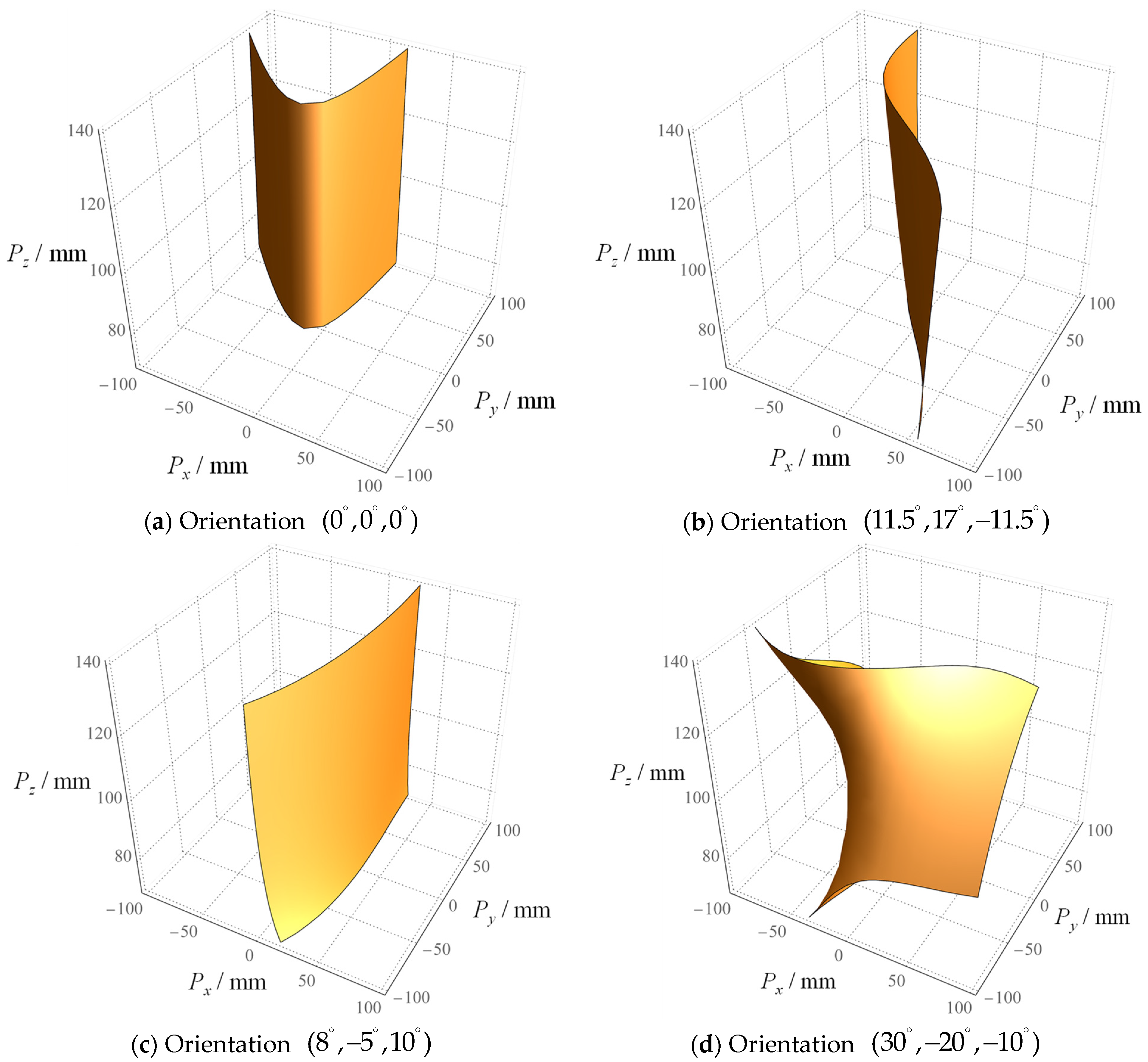
Figure 12 shows the singular trajectory of the isolator’s three-dimensional position with different orientation parameters. In Figure 12a, the singular trajectory is a continuous surface with larger curvature and more regular shape when the moving platform is not twisted. Figure 12b,c are position-singular trajectories for the orientation parameters given in Section 4.2. When the orientation angle is small, the curvature and range of the position-singular surface is small, so it is easy to avoid. Figure 12d shows the position of the singular trajectory surface when the orientation parameter is large, and the surface is large and complex. Thus, when the orientation parameters of the moving platform are small, it can be seen that the singular deformation does not easily occur.

5.3. Orientation-Singularity Analysis

The orientation-singularity trajectory is $\mathit{R}\in \mathrm{SO}(4)$ when the positioning parameters $P_x$, $P_y$, $P_z$ are given. Therefore, the expression of the position-singularity trajectory of the vibration isolator is expressed as:

$$\begin{array}{l}\det ({\mathit{J}}_x^q)=f_1^d{q}_{r0}{}^8+f_2^d{q}_{r1}{}^8+f_3^d{q}_{r2}{}^8+f_4^d{q}_{r3}{}^8+f_5^d{q}_{r0}{q}_{r1}{}^7+f_6^d{q}_{r1}{q}_{r2}{}^7+\mathsf{\Lambda }+\\ f_{160}^d{q}_{r0}{}^5{q}_{r1}{q}_{r2}{q}_{r3}+f_{161}^d{q}_{r0}{q}_{r1}{}^5{q}_{r2}{q}_{r3}+f_{162}^d{q}_{r0}{q}_{r1}{q}_{r2}{}^5{q}_{r3}+f_{163}^d{q}_{r0}{q}_{r1}{q}_{r2}{q}_{r3}{}^5+f_{164}^d=0\end{array}$$

(50)

where ${\mathit{f}}_i^d$, $(i=1,2,\cdots ,164)$ is the display expression of position parameters $P_x$, $P_y$, and $P_z$ and the vibration isolator size parameters.

Figure 13 shows the orientation-singular trajectory when the isolator is located at different positions. The blue area of the surface is the orientation-singular trajectory, which is more complex and discontinuous than the position-singular trajectory. Under different position parameters, the singular trajectory curves of 6-DOF isolators have no obvious geometric properties. However, the rule that the singular trajectory will not pass through the orientation origin at any given position is satisfied. Thus, in theory, there must be a non-singular orientation space near the orientation origin.

5.4. Discussion

The kinematics and dynamics performance decrease sharply when the 6-DOF isolator is located in a singular configuration. Thus, the 6-DOF isolator should be far away from the singular configuration work. In a mechanical structure, the closest explanation of singularity concerns the dead point of the structure. The position-singularity does not easily occur when the orientation parameters of the moving platform are small, as can be seen from the results in Section 5.2. Firstly, the difference in the length of each leg increases when the orientation angle increases. It is easy to make the moving platform and the outrigger collinear when the moving platform moves. Thus, the structure appears at the dead point and the singularity phenomenon occurs. Similarly, the conclusion of Section 5.3 can be well understood using this point of view. In the case of a given non-singular position, there must be a non-singular orientation space near the orientation’s origin. Further research can judge the orientation capability of the structure by calculating the size of the orientation space.

6. Conclusions

Given the extreme reduction in environment vibration and the isolation of some aircraft equipment, a 6-DOF all-metal vibration isolator with rectangular spring and annular metal rubber in symmetrical arrangement was designed and developed. Under the installation and stiffness requirements, the platform size and the operating range of a single damping-reducing outrigger were determined, and its kinematics and singularity were analyzed. The main conclusions are as follows:

(1)

Under the representation of dual quaternions, the forward kinematics model of the 6-DOF isolator can be rewritten in quadratic form.

(2)

Compared with the traditional rotation-matrix and Newton–Raphson methods, the computational efficiency of the enhanced Broyden numerical iterative algorithm increased by 680% and 290%, respectively.

(3)

The position-singularity does not easily occur when the orientation parameters of the moving platform are small. The orientation-singularity does not pass through the orientation origin. In addition, in theory, there must be a non-singular orientation space near the orientation origin.

References

- Zou, L.; Zheng, C.; Zheng, Z.; Hu, F.; Shao, Y.; Xue, X. Comparison of Dynamic Performance of an All-Metallic Vibration Isolator by Elliptic Method and Frequency Sweeping Method. Symmetry 2022, 14, 2017. [Google Scholar] [CrossRef]
- Yang, P.; Bai, H.; Xue, X.; Xiao, K.; Zhao, X. Vibration reliability characterization and damping capability of annular periodic metal rubber in the non-molding direction. Mech. Syst. Signal Process. 2019, 132, 622–639. [Google Scholar] [CrossRef]
- Gexue, R.; Qiuhai, L.; Ning, H.; Rendong, N.; Bo, P. On vibration control with Stewart parallel mechanism. Mechatronics 2004, 14, 1–13. [Google Scholar] [CrossRef]
- He, Z.; Feng, X.; Zhu, Y.; Yu, Z.; Li, Z.; Zhang, Y.; Wang, Y.; Wang, P.; Zhao, L. Progress of Stewart Vibration Platform in Aerospace Micro–Vibration Control. Aerospace 2022, 9, 324. [Google Scholar] [CrossRef]
- Hu, F.; Jing, X. A 6-DOF passive vibration isolator based on Stewart structure with X-shaped legs. Nonlinear Dyn. 2018, 91, 157–185. [Google Scholar] [CrossRef]
- Stewart, D. A platform with six degrees of freedom. Proc. Inst. Mech. Eng. 1965, 180, 371–378. [Google Scholar] [CrossRef]
- Zhou, W.; Chen, W.; Liu, H.; Li, X. A new forward kinematic algorithm for a general Stewart platform. Mech. Mach. Theory 2015, 87, 177–190. [Google Scholar] [CrossRef]
- Jang, T.K.; Lim, B.S.; Kim, M.K. The canonical stewart platform as a six DOF pose sensor for automotive applications. J. Mech. Sci. Technol. 2018, 32, 5553–5561. [Google Scholar] [CrossRef]
- Allred, C.J.; Jolly, M.R.; Buckner, G.D. Real-time estimation of helicopter blade kinematics using integrated linear displacement sensors. Aerosp. Sci. Technol. 2015, 42, 274–286. [Google Scholar] [CrossRef]
- Cheng, S.; Liu, Y.; Wu, H. A new approach for the forward kinematics of nearly general Stewart platform with an extra sensor. J. Adv. Mech. Des. Syst. Manuf. 2017, 11, JAMDSM0032. [Google Scholar] [CrossRef] [Green Version]
- Liu, Y.; Cheng, S.; Jiang, S.; Yang, X.; Li, Y.; Wu, H. Forward kinematics of 6-UPS parallel manipulators with one displacement sensor. J. Mech. Eng. 2018, 54, 1–7. [Google Scholar] [CrossRef]
- Boutchouang, A.H.B.; Melingui, A.; Ahanda, J.J.B.M.; Lakhal, O.; Motto, F.B.; Merzouki, R. Forward Kinematic Modeling of Conical-Shaped Continuum Manipulators. Robotica 2021, 39, 1760–1778. [Google Scholar] [CrossRef]
- Ma, J.; Chen, Q.; Yao, H.; Chai, X.; Li, Q. Singularity analysis of the 3/6 Stewart parallel manipulator using geometric algebra. Math. Methods Appl. Sci. 2018, 41, 2494–2506. [Google Scholar] [CrossRef]
- Wang, M.; Chen, Q.; Liu, H.; Huang, T.; Feng, H.; Tian, W. Evaluation of the Kinematic Performance of a 3-RRS Parallel Mechanism. Robotica 2021, 39, 606–617. [Google Scholar] [CrossRef]
- Zhu, G.; Wei, S.; Zhang, Y.; Liao, Q. A Novel Geometric Modeling and Calculation Method for Forward Displacement Analysis of 6-3 Stewart Platforms. Mathematics 2021, 9, 442. [Google Scholar] [CrossRef]
- Cheng, S.L.; Wang, C.Q.; Tao, Y.; Shu, J.Y. Analytical method for the forward kinematics analysis of the general 6-SPS parallel mechanisms. China Mech. Eng. 2010, 21, 1261–1264. [Google Scholar]
- Zhang, Y.; Liu, X.; Wei, S.; Wang, Y.; Zhang, X.; Zhang, P.; Liang, C. A Geometric Modeling and Computing Method for Direct Kinematic Analysis of 6-4 Stewart Platforms. Math. Probl. Eng. 2018, 2018, 6245341. [Google Scholar] [CrossRef]
- Merlet, J.P. Solving the Forward Kinematics of a Gough-Type Parallel Manipulator with Interval Analysis. Int. J. Robot. Res. 2004, 23, 221–235. [Google Scholar] [CrossRef]
- Yao, R.; Zhu, W.; Huang, P. Accuracy analysis of Stewart platform based on interval analysis method. Chin. J. Mech. Eng. 2013, 26, 29–34. [Google Scholar] [CrossRef]
- Zhou, X.; Xian, Y.; Chen, Y.; Chen, T.; Yang, L.; Chen, S.; Huang, J. An improved inverse kinematics solution for 6-DOF robot manipulators with offset wrists. Robotica 2022, 40, 2275–2294. [Google Scholar] [CrossRef]
- Song, G.; Su, S.; Li, Y.; Zhao, X.; Du, H.; Han, J.; Zhao, Y. A Closed-Loop Framework for the Inverse Kinematics of the 7 Degrees of Freedom Manipulator. Robotica 2021, 39, 572–581. [Google Scholar] [CrossRef]
- Guo, D.; Li, A.; Cai, J.; Feng, Q.; Shi, Y. Inverse kinematics of redundant manipulators with guaranteed performance. Robotica 2022, 40, 170–190. [Google Scholar] [CrossRef]
- Luo, R.; Gao, W.; Huang, Q.; Zhang, Y. An improved minimal error model for the robotic kinematic calibration based on the POE formula. Robotica 2022, 40, 1607–1626. [Google Scholar] [CrossRef]
- Yin, F.; Wang, L.; Tian, W.; Zhang, X. Kinematic calibration of a 5-DOF hybrid machining robot using an extended Kalman filter method. Precis. Eng. 2023, 79, 86–93. [Google Scholar] [CrossRef]
- Luo, Y.; Gao, J.; Zhang, L.; Chen, D.; Chen, X. Kinematic calibration of a symmetric parallel kinematic machine using sensitivity-based iterative planning. Precis. Eng. 2022, 77, 164–178. [Google Scholar] [CrossRef]
- Geng, M.; Zhao, T.; Wang, C. Direct position analysis of parallel mechanism based on quasi-Newtonmethod. J. Mech. Eng. 2015, 51, 28–36. [Google Scholar] [CrossRef]
- Yang, X.L.; Wu, H.T.; Chen, B.; Zhu, L.C.; Xun, J.X. Fast Numerical solution to forward kinematics of general Stewart mechanism using quaternion. Trans. Nanjing Univ. Aeronaut. Astronaut. 2014, 31, 377–385. [Google Scholar]
- Yang, F.; Tan, X.; Wang, Z.; Lu, Z.; He, T. A Geometric Approach for Real-Time Forward Kinematics of the General Stewart Platform. Sensors 2022, 22, 4829. [Google Scholar] [CrossRef]
- Masory, O.; Wang, J.; Zhuang, H. On the accuracy of a Stewart platform—Part 2: Kinematic calibration and compensation. In Proceedings of the 1993 IEEE International Conference on Robotics and Automation, Atlanta, GA, USA, 2–6 May 1993; pp. 725–731. [Google Scholar]
- Yang, S.; Li, Y. Classification and analysis of constraint singularities for parallel mechanisms using differential manifolds. Appl. Math. Model. 2020, 77, 469–477. [Google Scholar] [CrossRef]
- Yang, X.; Wu, H.; Chen, B.; Li, Y.; Jiang, S. A dual quaternion approach to efficient determination of the maximal singularity-free joint space and workspace of six-DOF parallel mechanisms. Mech. Mach. Theory 2018, 129, 279–292. [Google Scholar] [CrossRef]
- Su, Y.; Duan, B.; Peng, B.; Nan, R. Singularity analysis of fine-tuning Stewart platform for large radio telescope using genetic algorithm. Mechatronics 2003, 13, 413–425. [Google Scholar] [CrossRef]
- Lacombe, L.; Gosselin, G. Singularity analysis of a kinematically redundant (6+2)-DOF parallel mechanism for zero-torsion configurations. Mech. Mach. Theory 2022, 170, 104682. [Google Scholar] [CrossRef]
- Schappler, M.; Ortmaier, T. Singularity avoidance of task-redundant robots in pointing tasks: On null space projection and cardan angles as orientation coordinates. In Proceedings of the 18th International Conference on Informatics in Control, Automation and Robotics (ICINCO 2021), Online Streaming. 6–8 July 2021; SciTePress: Setúbal, Portugal, 2021; pp. 338–349. [Google Scholar]
Figure 1.
Structure diagram of a 6-DOF all-metal vibration isolator.
Figure 2.
Internal structure diagram of the damping-reducing outrigger.
Figure 3.
Simplified structure diagram of the proposed 6-DOF all-metal vibration isolator.
Figure 4.
Euler angle conversion between moving and static coordinates ( and ).
Figure 5.
The closed-loop of the outrigger schematic diagram.
Figure 6.
The theoretical stiffness ratio curve for a three-dimensional vibration isolator.
Figure 7.
Procedure of the forward kinematic algorithm.
Figure 8.
Schematic of position and orientation for a 6-DOF all-metal vibration isolator.
Figure 9.
Iterative process of 6-DOF all-metal vibration isolator.
Figure 10.
Iterative process of the traditional Euler angle method.
Figure 11.
Iterative process of the Newton–Raphson method.
Figure 12.
Position-singularity vibration isolator for different orientations.
Figure 13.
Orientation-singularity vibration isolator for different positions.
Disclaimer/Publisher’s Note: The statements, opinions and data contained in all publications are solely those of the individual author(s) and contributor(s) and not of MDPI and/or the editor(s). MDPI and/or the editor(s) disclaim responsibility for any injury to people or property resulting from any ideas, methods, instructions or products referred to in the content. |
© 2023 by the authors. Licensee MDPI, Basel, Switzerland. This article is an open access article distributed under the terms and conditions of the Creative Commons Attribution (CC BY) license (https://creativecommons.org/licenses/by/4.0/).
Share and Cite
MDPI and ACS Style
Zheng, C.; Zou, L.; Zheng, Z.; Xue, X. Kinematics Modeling and Singularity Analysis of a 6-DOF All-Metal Vibration Isolator Based on Dual Quaternions. Symmetry 2023, 15, 562. https://0-doi-org.brum.beds.ac.uk/10.3390/sym15020562
AMA Style
Zheng C, Zou L, Zheng Z, Xue X. Kinematics Modeling and Singularity Analysis of a 6-DOF All-Metal Vibration Isolator Based on Dual Quaternions. Symmetry. 2023; 15(2):562. https://0-doi-org.brum.beds.ac.uk/10.3390/sym15020562
Chicago/Turabian StyleZheng, Chao, Luming Zou, Zhi Zheng, and Xin Xue. 2023. "Kinematics Modeling and Singularity Analysis of a 6-DOF All-Metal Vibration Isolator Based on Dual Quaternions" Symmetry 15, no. 2: 562. https://0-doi-org.brum.beds.ac.uk/10.3390/sym15020562
Note that from the first issue of 2016, this journal uses article numbers instead of page numbers. See further details here.