Article

Dynamical Response of Particles in Asymmetric Ratchet Potential

by
Usman A. Marte
1,*,
Uchechukwu E. Vincent
2,3,*,†,
Abdulahi N. Njah
4,5,† and
Biodun S. Badmus
4,†
1
Department of Mathematics and Statistics, University of Maiduguri, P.M.B. 1069 Maiduguri, Nigeria
2
Department of Physics, Lancaster University of Lancaster, Lancaster LA1 4YB, UK
3
Department of Physical Sciences, Redeemer's University, P.M.B. 3005 Redemption City, Nigeria
4
Department of Physics, Federal University of Agriculture, P.M.B. 2240 Abeokuta, Nigeria
5
Department of Physics, University of Lagos, P.M.B. 56 Akoka-Yaba, Lagos, Nigeria
*
Authors to whom correspondence should be addressed.
These authors contributed equally to this work.
Submission received: 28 July 2014 / Revised: 23 September 2014 / Accepted: 15 October 2014 / Published: 27 October 2014

Abstract

:
The dynamics and response of particles in an asymmetric potential of the ratchet type is considered. An approximate asymmetric ratchet potential, which allows us to apply an analytical approach to investigate the systems’ response, is proposed based on the power series interpolation scheme. The method of multiple scales (MMS) is then employed to obtain an approximate solution at the principal resonance. Comparison between results obtained from the approximated and exact potentials show excellent agreement. The frequency response curves (FRCs) for different forcing are presented. The numerically computed FRCs were compared with the theoretical result to show the extent of agreement. Furthermore, by using perturbation methods, the stable and unstable domains of the solution were obtained.

Graphical Abstract

1. Introduction

In recent times, there has been increasing interest in the study of the transport properties of nonlinear systems that extract usable work from unbiased non-equilibrium fluctuations [1]; one of the reasons being that non-equilibrium dynamical systems are potential models for describing a wide range of natural and mechanical systems [2]. For instance, rectifying the motion of the Josephson phase in superconducting quantum interference devices (SQUIDs) or long Josephson junctions, vortices in superconductors and Josephson junction arrays are some physical promising implementations of a ratchet device (see [3] and the references therein).
In general, a ratchet can be modelled, for instance, by considering a Brownian particle in a periodic asymmetric potential, which is acted upon by an external time-dependent force of zero average. The basic concept is governed by the second law of thermodynamics, wherein noise-induced directed transport in a spatially periodic system in thermal equilibrium is ruled out [4,5]. Therefore, to generate transport, Brownian motors or ratchet devices could be used for modelling such systems. Interestingly, deterministically-induced chaos could in many instances mimic the role of noise, thereby steering the system to exhibit current flow in either direction. Within this framework, diverse research works, ranging from chaotic transport and transport control via nonlinear control theory, to control by synchronization, have been done [525].
Despite the huge research progress made in the study of ratchet systems to date, only a few recent works reported the response of particles in asymmetric ratchet potential. For instance, Nana-Nbendjo et al. [24] carried out an analytical study of its stability, examined resonance oscillations for two indirectly-coupled ratchets and reported the existence of multi-resonance. In a very recent and related work, Vincent et al. [25] considered the collective dynamics of a network of particles in a ratchet potential and observed collective resonance. Remarkably, these works were mainly concerned with numerical results, with no recourse to the analytical treatment of the frequency response.
In this paper, we propose an approach that allows us to obtain, analytically and numerically, the dynamical response of a deterministic (i.e., noiseless) inertia ratchet system by means of a polynomial interpolation scheme. Our motivations for investigating deterministic ratchets transporting massive particles is derived from the strong inertial effects leading to current reversals, as well as their natural capability for developing chaotic dynamics; all of which, in nanotechnology, makes it a practical, viable alternative for the purpose of rectification (see [3] and the references therein). Indeed, it was pointed out that the inertia system can perform more effectively and efficiently than the more popular over-damped Brownian motors originally inspired by cellular biology [3]. On the other hand, the need for polynomial interpolation has been informed by the need to re-express the ratchet potential containing the sine functions in a form that will be readily accessible to analytical treatment using the method of multiple timescales (MMS). Application of the MMS involves the composition of an exponential function of these sine functions, which makes the solvability conditions difficult to obtain. Thus, the problem was easily overcome by means of the polynomial approximation. With our proposed approach, we obtain an approximate asymmetric ratchet potential, which allows us to apply the method of multiple scales in order to obtain the frequency response analytically and then confirm the result by direct numerical solution of the nonlinear base equation.
The rest of the paper is organized as follows. In the next section, we give a brief description of the inertia ratchet model. Section 3 describes our approximation technique, an analysis using the method of multiple scales, as well as the examination of the stability of the steady state of the attractors. The paper is concluded in Section 4.

2. The Inertia Ratchet

Consider the one-dimensional equation of motion of a particle driven by a periodic time-dependent external force under the influence of an asymmetric potential of the ratchet type. The time average of the external deterministic force is zero, and the dimensionless equation of motion is given by [525]:
x ¨ + b 1 x ˙ + d V ( x ) d x = F 0 cos ( ω t )
where b1 is a dimensionless friction coefficient, F0 is the amplitude of the external forcing, ω is the external driving frequency and V(x) is an external asymmetric periodic potential of the ratchet type given by [6] as:
  V ( x ) = c 1 4 π 2 δ [ sin ( 2 π ( x x 0 ) ) + 0.25 sin ( 4 π ( x x 0 ) ) ]
where the potential is shifted by x0 in order to make the minima of the potential to be located at integer values. The parameters δ = 1.61432 and c = 0.0173. System (1) has been extensively studied in both the low [26] and moderate [9,1113] damping regimes, where chaotic, as well as regular dynamics could be found; while in [27,28], the effects of noise were investigated. In order to facilitate the analysis using the method of multiple scales, Equation (1) may be written as:
x ¨ + ω 0 2 x = b 1 x ˙ + 1 4 π δ [ 2 cos ( 2 π ( x x 0 ) ) + cos ( 4 π ( x x 0 ) ) ] + ω 0 2 x + F 0 cos ω t
where ω0 is the natural frequency of the system.

3. Results and Discussion

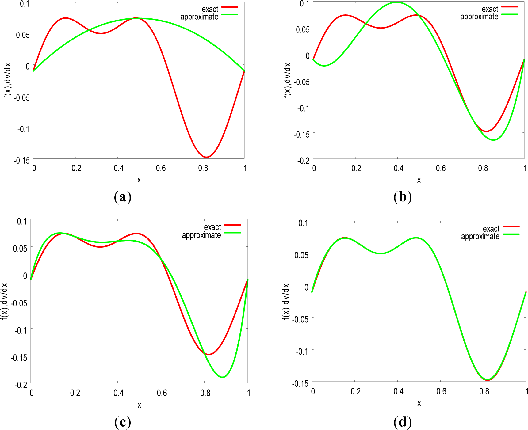
3.1. Approximation Technique

Our goal is to seek for an approximate asymptotic solutions of Equation (3) using multiple scales [29,30]. In order to achieve this, we first obtain an approximation to the potential given by Equation (2) by considering a set of N + 1 data points, from which we fit an N-th degree polynomial that passes through these points by means of the Lagrange interpolating functions. Regardless of how the N-th degree polynomial is constructed, the resulting polynomial would be the same. Now, let g(x) be the exact function, with known N + 1 discrete values used to establish an interpolating polynomial or approximating function f(x). The function f(x) should pass through all specified N + 1 points, also referred to as data points or nodes. For a given set of interpolating points (xi, g(xi) = gi, i = 0, …, N), there exists only one polynomial that passes through a given set of N + 1 points. Its form, expressed in power series, is given by:
f ( x ) = i = 0 N a i x i
where ai(i = 0, 1, 2, …, N + 1) are unknown coefficients. In principle, f(x) must match g(x) at the selected data points, such that:
( x j : f ( x j ) = g j = k = 0 N a j x j k , { j = 1 , , N } )
From the above matrix, the unknown coefficients ai can be obtained. The second term on the right-hand side of Equation (3) represents dV/dx. To obtain the approximation, we choose evenly-spaced data points and evaluate the coefficients ai from Equation (5).
We begin by dividing the interval [0,1] into two equal sub-intervals, so that the interpolating polynomial becomes f(x) = a0 + a1x + a2x2, where a0 = −0.0105557, a1 = 0.335818, a2 = −0.335818. Next, we consider four sub-intervals and obtain the interpolating polynomial as f(x) = a0 + a1x + a2x2 + a3x3 + a4x4, where a0 = −0.0105557, a1 = −0.501061, a2 = 5.75165, a3 = −12.4042, a4 = 7.15365. For five sub-intervals, the interpolating polynomial becomes f(x) = a0 + a1x + a2x2 + a3x3 + a4x4 + a5x5, where a0 = −0.0105557, a1 = 1.69548, a2 = −11.7413, a3 = 34.1655, a4 = −43.5321, a5 = 19.4124.
Finally, for ten sub-intervals, we obtain the interpolating polynomial:
f ( x ) = a 0 + a 1 x + a 2 x 2 + a 3 x 3 + a 4 x 4 + a 5 x 5 + a 6 x 6 + a 7 x 7 + a 8 x 8 + a 9 x 9 + a 10 x 10
From Equation (5), the following values of ai were obtained: a0 = −0.0105557, a1 = 1.31333, a2 = −9.63468, a3 = 77.7829, a4 = −571.273, a5 = 2424.3, a6 = −5748.15, a7 = 7839.35, a8 = −6123.42, a9 = 2547.15 and a10 = −437.428. With further division of the interval to twenty equal sub-intervals, the interpolating polynomial becomes “drowned” in its rounding errors. Remarkably, when the component of V(x) with a half period is set to zero, the dynamics of System (1) could simply be likened to a model of a superconducting Josephson junction considered by Huberman et al. [31]. However, in this limit, and for a 2π periodic potential function, as in [31], the best polynomial fit can be obtained using eighth-order polynomial by dividing the 2π periodic function into eight equal parts.
In the following analysis, we choose the case of ten sub-intervals, which gives an excellent agreement, and a prime period of the system is considered, which can be extended to infinitum by the use of the Mod[x,1] in the interpolating polynomial obtained in Equation (6). To validate the above result, we first compare the approximated dV/dx with the results obtained by direct numerical simulation, as shown in Figure 1, where we superpose the plots for the exact (red lines) and the approximation (green lines) obtained using Equation (6) in the interval 0 ≤ x ≤ 1. The interpolating polynomial can be extended to infinitum by the use of the Mod function. Clearly, one can see an excellent qualitative agreement between the two plots.
First, we computed the chaotic attractor using Equation (1) with the exact potential (2) and compare with the attractor obtained using potential (6). Clearly, as shown in Figure 2, the two attractors (exact in green and approximated in read) are qualitatively in good agreement, retaining the essential features, including the shapes, basins and boundedness of the attractor.

3.2. Analysis with the Method of Multiple Scales

Now, considering Equations (1) and (6), one seeks for asymptotic solutions by employing the method of multiple scales [26,32]. For a small, but finite, value of x, one considers a power series solution of the form:
x ( t : ε ) = x 0 ( T 0 , T 1 ) + ε x 1 ( T 0 , T 1 ) +
where T0 = t a is a fast scale and T1 = εt is a slow scale. The first and second derivatives are given by:
d d t = D 0 + ε D 1 + ,    d 2 d t 2 = D 0 2 + 2 ε D 0 D 1
Equating the coefficients of equal powers of ε results in O(ε0) and O(ε1), we obtain respectively,
D 0 2 x 0 + ω 0 2 x 0 = 0
and
D 0 2 x 1 + ω 0 2 x 1 = 2 D 0 D 1 x 0 b D 0 x 0 + F 0 cos ( ω t ) + α f ( x 0 ) + ω 0 2 x 0
The general solution of Equation (10) can be written in the form:
x 0 = A ( T 1 ) e i ω 0 T 0 + A ¯ ( T 1 ) e i ω 0 T 0
where α = εα10, ω0 = εω10, b = εb1; ω10 and α10 are the natural frequency and scaling factor, respectively.
The complex conjugate pair quantities A(T1) and Ā(T1) are arbitrary functions, to this order of approximation, and are determined by imposing the solvability conditions in the next order of approximation. Substituting Equation (11) into Equation (10) results in:
D 0 2 x 1 + ω 0 2 x 1 = ( i ω 0 ( 2 A b A ) + α J 1 ( A ) + ω 0 2 ) e i ω 0 T 0 + α ( J 2 ( A ) e 2 i ω 0 T 0 + J 3 ( A ) e 3 i ω 0 T 0 + J 4 ( A ) e 4 i ω 0 T 0 + J 5 ( A ) e 5 i ω 0 T 0 + J 6 ( A ) e 6 i ω 0 T 0 J 7 ( A ) e 7 i ω 0 T 0 + J 8 ( A ) e 8 i ω 0 T 0 + J 9 ( A ) e 9 i ω 0 T 0 + J 10 ( A ) e 10 i ω 0 T 0 + J 11 ( A ) ) + 1 2 F 0 e i ω T 0
The quantities Ji(A), i = 1, 2, …, 12 are defined in the Appendix.

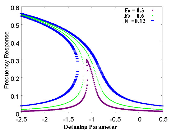
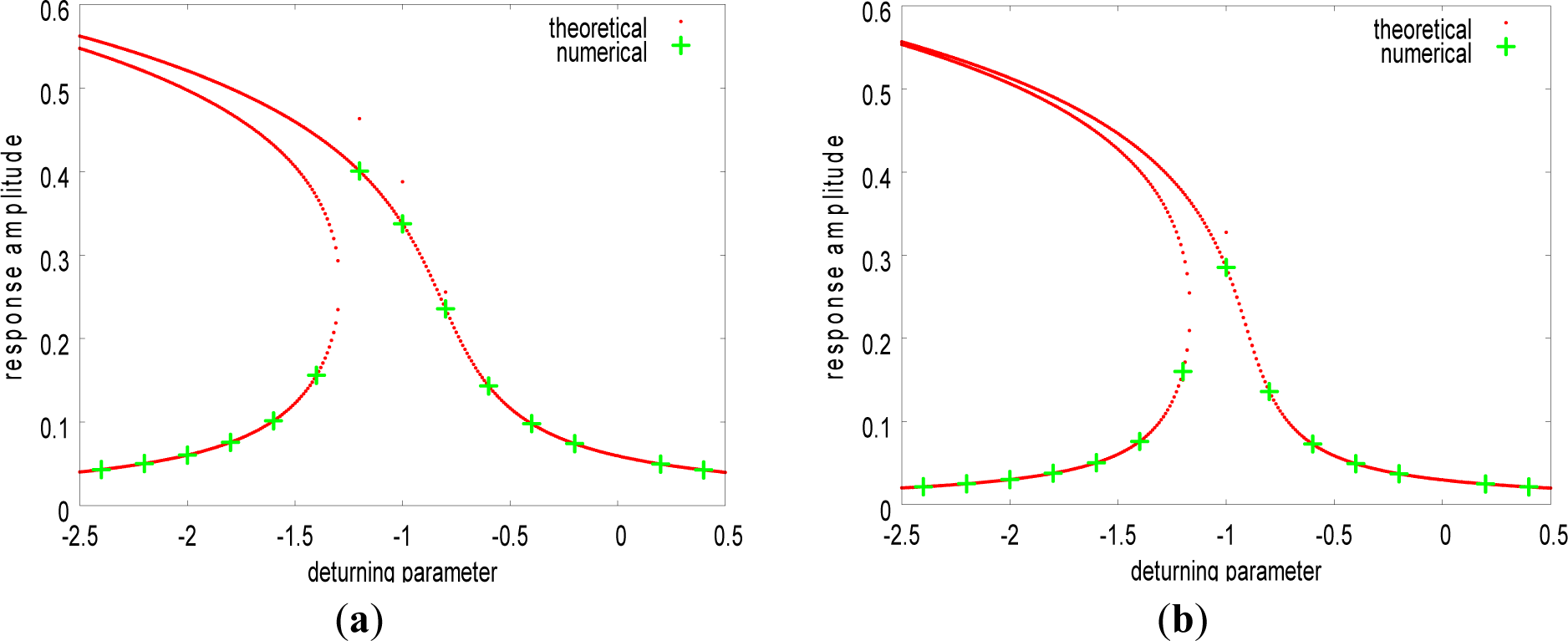
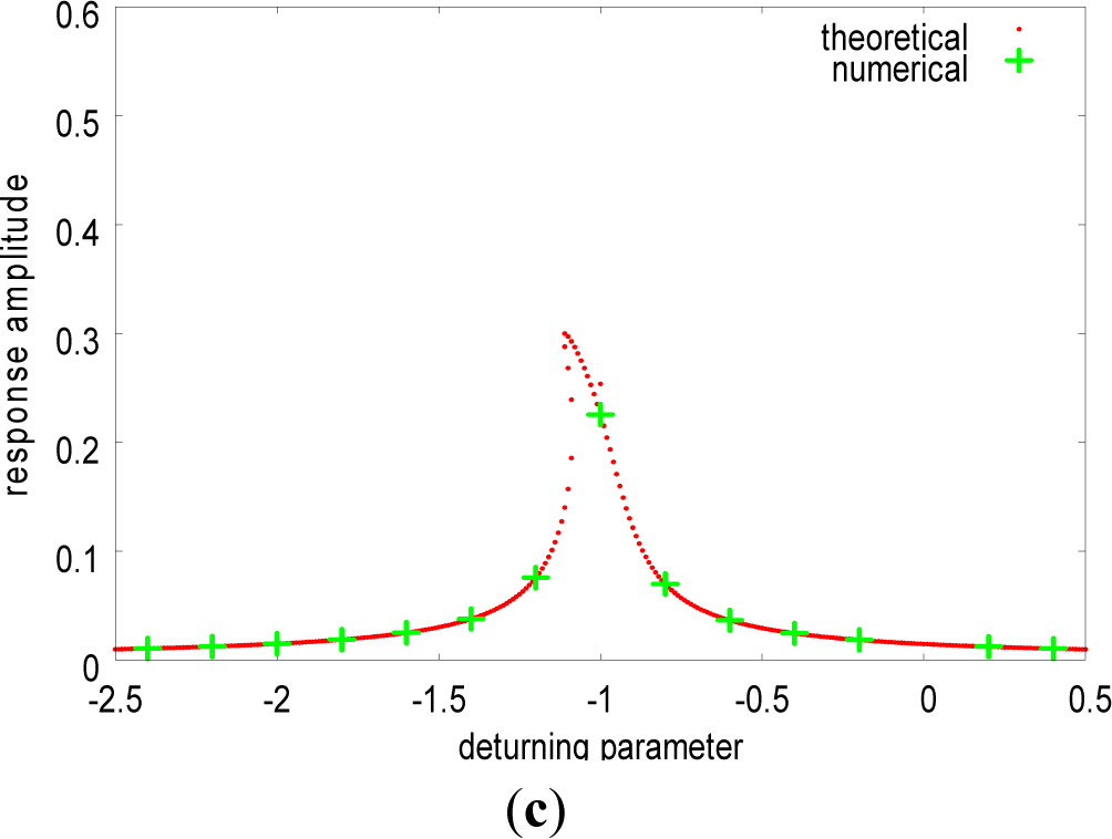
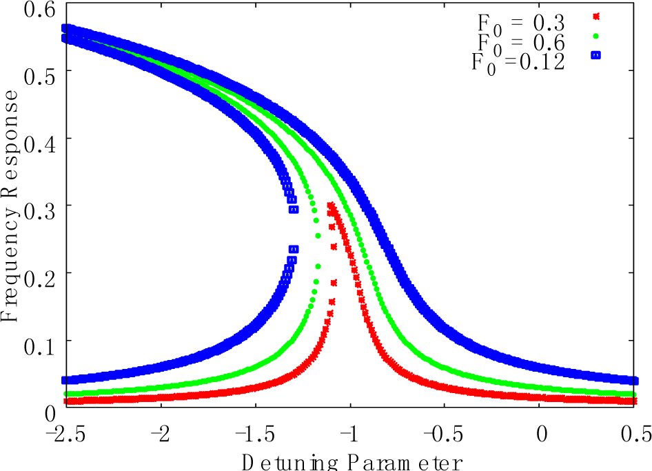
3.3. Principal Resonance

Here, we analyse the case where ω0 is close to ω; where we set ω = ω0 + εσ and σ is the detuning parameter. For a bounded solution, one has to impose a condition to eliminate secular terms in Equation (12). This requires that:
D 0 2 x 1 + w 0 2 x 1 = ( i w 0 ( 2 A b 1 A ) + w 0 2 A + J 1 ( A ) ) e i w 0 T 0 + [ H . O . T ] + 1 2 F 0 e i w T 0
where [H.O.T] refer to higher order terms in e i w 0 T 0. To solve Equation (13) A is written in polar form as:
A ( T 1 ) = 1 2 a e i φ
where a and φ are real functions. Substituting Equation (14) in Equation (13) results in:
i ω 0 ( a + i a φ ) 0.5 i ω 0 b 1 a + α s ( a ) + ω 0 2 a + F 0 2 e i ( σ T 1 φ )
where s(a) = 0.65667a + 29.16859a3 + 757.59375a5 + 2143.57227a7 + 626.8377a9.
Separating real and imaginary parts results in the following Equations:
a = b 1 2 a + F 0 2 ω 0 sin θ a θ = a σ + α 2 ω 0 s ( a ) + ω 0 2 a + F 0 2 ω 0 cos θ
where θ = σT1 – φ. The stability of the solution can be examined by locating the singular points and their neighbourhoods. When the amplitude and the phase do not change at the singular points, the response is said to be a steady-state motion. From Equation (16), the position and velocity of the particle can be found at any point in time, thus enabling the knowledge of the particles’ current at any point in time.
The steady-state motion occurs when a′ = θ′ = 0 and φ′ = σ, which corresponds to the singular points of Equation (16), which, in turn, correspond to the solutions of:
1 2 b 1 a = F 0 2 ω 0 sin θ a σ + α 2 ω 0 s ( a ) + ω 0 2 a = F 0 2 ω 0 cos θ
By squaring and adding the Equations in (17), we obtain the expression for the frequency response as:
ω 0 2 b 1 2 a 2 + 4 ω 0 2 [ σ a + α ω 0 s ( a ) + ω 0 a ] 2 = F 0 2
Equation (18) is an implicit equation for the amplitude of the response as a function of the detuning parameter σ (frequency of the excitation) and the amplitude of the excitation, which is called the frequency response. By fixing the system parameters as b1 = 0.1, ω0 = 1.0, α = 0.01, we show a plot of the frequency response curves for different values of the external excitation amplitude, F0 = 0.03, 0.06 and 0.12. The theoretical and the numerical response amplitude are first compared from Equations (16) and (18). Again, we find excellent agreement, as shown in Figure 3.
By comparing the frequency response curves for different values of the external excitation amplitude, F0 = 0.03, 0.06 and 0.12, we observe, clearly, a jump phenomenon for some values of the forcing amplitude F0. As shown in Figure 4, the jump phenomenon is not visible at F0 = 0.03, but at F0 = 0.06. At higher values of F0, the jump is clearly visible. Notably, as F0 increases, the point at which the jump occurs moves away from the resonance point (i.e., at σ = −1), as shown in Figure 3. The occurrence of the jump phenomenon in the frequency resonance curve is evidence of the system’s strong dependency on the initial conditions. Strong dependence on the initial conditions is typical of deterministic underdamped ratchets [26].

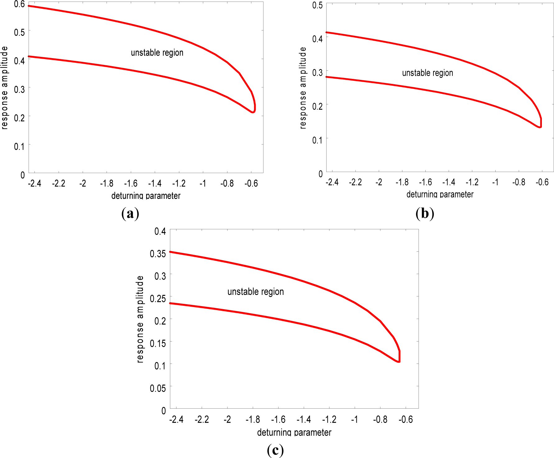
3.4. Stability of the Steady-State Solution

The stability of the steady-state motion can be examined from Equation (17) by introducing a small perturbation of the form:
a = a 0 + a 1 θ = θ 0 + θ 1
Substituting Equation (19) in Equation (17) and keeping only the linear terms in a1 and θ1, noting that a0 and θ0 satisfy Equation (18), results in the following:
a 1 = b 1 2 a 1 + [ F 0 2 ω 0 cos θ 0 ] θ 1 θ 1 = [ α a 0 2 ω 0 ( u ( a 0 ) s ( a 0 ) ) F 0 2 a 0 ω 0 cos θ 0 ] a 1 [ F 0 2 ω 0 a 0 sin θ 0 ] θ 1
where u ( a ) = 1 2 a 1 a + 3 3 8 a 3 a 3 + 5 10 32 a 5 a 5 + 7 35 128 a 7 a 7 + 9 126 512 a 9 a 9.
Thus, the stability of the steady-state motion depends on the eigenvalues of the coefficient matrix of the right-hand side of Equation (21), given by the equation:
| b 1 2 λ 1 ω 0 ( a 0 σ + α s ( a 0 ) + ω 0 2 a 0 ) α u ( a 0 ) + 1 ω 0 a 0 2 ( a 0 σ + α s ( a 0 ) + ω 0 2 a 0 ) b 1 2 λ | = 0
Choose the values ω0 = 1.0, α = 0.01 and b1 = 0.1. In order to obtain the stability conditions, we employ the Routh–Hurwitz criterion. Given a polynomial:
P ( λ ) = λ n + a 1 λ n 1 + + a n 1 λ + a n
where the coefficients ai, i = 1, 2, 3, … n, are real constants. Define as Hurwitz the n matrices using the coefficients ai of the characteristics polynomial:
H 1 ( a 1 ) = ( a 1 ) , H 2 = ( a 1 1 a 3 a 2 ) , H 3 = ( a 1 1 0 a 3 a 2 a 1 a 5 a 4 a 3 ) and H n = ( a 1 1 0 0 0 a 3 a 2 a 1 1 0 a 5 a 4 a 3 a 2 0 0 0 0 0 a n )
where ai = 0 if j > n. All of the roots of the polynomials P(λ) are negative or have a negative real part if and only if the determinants of all of the Hurwitz matrices are positive: det. Hj > 0, j = 1, 2, …, n. When n = 2, the Routh–Hurwitz criterion simply becomes det. H1 = a1 > 0 and det. H 2 = det ( a 1 1 a 3 a 2 ) = a 1 a 2 > 0 or a 1> 0 and a2 > 0 and a3 = 0 by definition. Applying the above criteria to our system Equation (21) results in the stability condition given by:
b 1 2 4 + ( α u ( a 0 ) + 1 a 0 2 ( a 0 σ + α s ( a 0 ) + ω 0 2 a 0 ) ) ( a 0 σ + α s ( a 0 ) + ω 0 2 a 0 ) > 0
By choosing the following parameter values, ω0 = 1.0, α = 0.01 and b1 = 0.1, we show in Figure 5 the variation of the stability boundaries with increasing nonlinearity α. The stability analysis and the numerical solutions (green points) in Figure 3 show clearly the realizable values of the amplitudes where abrupt changes in a very small window of the detuning parameter can take place. This relates to the result reported in [26], where a sudden jump in the current in a very narrow rectification amplitude window was reported.

4. Conclusions

In this paper, we studied the dynamics of a deterministic inertia ratchet system subjected to an external periodic forcing. This system is extremely sensitive to initial conditions and has a natural capability for exhibiting chaotic dynamics, which in practice makes it a suitable model in nanotechnology for the purpose of rectification [3]. Due to this strong nonlinear property, it can perform more effectively and efficiently than the popular over-damped models that find useful applications in cellular biology [3]. Here, we have obtained the frequency response analytically by approximating the ratchet potential with a power series by means of an interpolation scheme. The method of multiple scales was used to obtain an analytic solution at the primary resonance. The frequency response shows evidence of sensitivity to initial conditions manifesting as jump phenomena at different amplitudes of the external forcing. Numerical solutions of the response amplitude were computed and compared with the theoretical results. The stability of the solution was analysed by perturbation methods to obtain the boundary separating the stable and the unstable regions using the Routh–Hurwitz criterion. The results showed that as the nonlinearity increases, the region of stability decreases. The realizable values of the amplitudes where abrupt changes in a very small window of the detuning parameter can take place were found. This is similar to the result reported in [26], where a sudden jump in the current in a very narrow rectification amplitude window was reported.

Author Contributions

Uchechukwu E. Vincent proposed the work. Usman A. Marte carried out all of the mathematical analysis under the joint supervision of Uchechukwu E. Vincent and Abdulahi N. Njah The code for Figure 2 was written by Uchechukwu E. Vincent. Manuscript preparation, presentation and editing were done by all of the authors.

Conflicts of Interest

The authors declare no conflict of interest.

Appendix

J 1 ( A ) = 0.0106 + ( 1.3133 A + 233.349 A 2 A ¯ + 24243 A 3 A ¯ 2 + 274377 A 4 A ¯ 3 + 320941 A 5 A ¯ 4 ) J 11 ( A ) = ( 19.2694 A A ¯ + 3427.64 A 2 A ¯ 2 + 114963 A 3 A ¯ 3 + 428639 A 4 A ¯ 4 + 110232 A 5 A ¯ 5 ) J 2 ( A ) = ( 9.6347 A 2 + 2285.09 A 3 A ¯ + 86222.3 A 4 A ¯ 2 + 342912. A 5 A ¯ 3 + 91859.8 A 6 A ¯ 4 ) J 3 ( A ) = ( 77.7829 A 3 + 12121.5 A 4 A ¯ + 164626 A 5 A ¯ 2 + 213961 A 6 A ¯ 3 ) J 4 ( A ) = ( 571.273 A 4 + 34488 A 5 A ¯ + 171456 A 6 A ¯ 2 + 52491.4 A 7 A ¯ 3 ) J 5 ( A ) = ( 2424.3 A 5 + 54875.5 A 6 A ¯ + 91697.4 A 7 A ¯ 2 ) J 6 ( A ) = ( 5748.15 A 6 + 48987.4 A 7 A ¯ + 19684.3 A 8 A ¯ 2 ) J 7 ( A ) = ( 7839 A 7 + 22924.4 A 8 A ¯ ) J 8 ( A ) = ( 6123.42 A 8 + 4374.28 A 9 A ¯ ) J 9 ( A ) = 2547.15 A 9 J 10 ( A ) = 437.428 A 10

Acknowledgments

Uchechukwu E. Vincent is supported by the Royal Society of London through their Newton International Fellowship Alumni scheme. We acknowledge and thank all of the reviewers for their constructive and critical comments that were very useful for improving the quality of this paper.

References

  1. Hanggi, P.; Marchesoni, F. Artificial Brownian transport on the nanoscale. Rev. Mod. Phys 2009, 81, 387–442. [Google Scholar]
  2. Julicher, F.; Ajdari, A.; Prost, J. Modelling molecular motors. Rev. Mod. Phys 1997, 69, 1269–1281. [Google Scholar]
  3. Marchesoni, F.; Savel’ev, S.; Nori, F. Achieving optimal rectification using underdamped rocked ratchets. Phys. Rev. E 2006, 73. [Google Scholar] [CrossRef]
  4. Astumian, R.D. Thermodynamics and kinetics of a Brownian motor. Science 1997, 276, 917–922. [Google Scholar]
  5. Reimann, P. Brownian Motors: Noisy Transport Far from Equilibrium. Phys. Rep 2002, 361, 57–265. [Google Scholar]
  6. Jung, J.; Kissner, J.G.; Hanggi, P. Regular and chaotic transport in asymmetric periodic potentials: Inertia ratchets. Phys. Rev. Lett 1996. [Google Scholar]
  7. Mateos, J.L. Chaotic transport and current reversal in deterministic ratchets. Phys. Rev. Lett 2000. [Google Scholar]
  8. Son, W.S.; Kim, I.; Park, Y.J.; Kim, C.M. Current reversal with type-I intermittency in deterministic inertia ratchets. Phys. Rev. E 2003, 68. [Google Scholar] [CrossRef]
  9. Barbi, M.; Salerno, M. Phase locking effect and current reversals in deterministic under-damped ratchets. Phys. Rev. E 2000. [Google Scholar]
  10. Kenfack, A.; Sweetnam, S.M.; Pattanayak, A.K. Bifurcations and sudden current change in ensembles of classically chaotic ratchets. Phys. Rev. E 2007, 75. [Google Scholar] [CrossRef]
  11. Mateos, J.L. Current reversals in deterministic chaotic ratchets. Phys. D 2002, 168–169, 205–219. [Google Scholar]
  12. Mateos, J.L. Current reversals in chaotic ratchets: The battle of attractors. Phys. A 2004, 325, 92–100. [Google Scholar]
  13. Mateos, J.L. Intermittency and deterministic diffusion in chaotic ratchets. Commun. Nonlinear Sci. Numer. Simul 2003, 8, 253–263. [Google Scholar]
  14. Vincent, U.E.; Njah, A.N.; Akinlade, O.; Solarin, A.R.T. Phase synchronization in unidirectionally coupled chaotic ratchets. Chaos 2004, 14, 1018–1025. [Google Scholar]
  15. Vincent, U.E.; Kenfack, A.; Njah, A.N.; Akinlade, O. Bifurcation and chaos in coupled ratchets exhibiting synchronized dynamics. Phys. Rev. E 2005, 72. [Google Scholar] [CrossRef]
  16. Kostur, M.; Hanggi, P.; Talkner, P.; Meteos, J.L. Anticipated synchronization in coupled inertia ratchets with time-delay feedback. Phys. Rev. E 2005, 72. [Google Scholar] [CrossRef]
  17. Vincent, U.E.; Laoye, J.A. Synchronization and control of directed trasnport in chaotic ratchets via active control. Phys. Lett. A 2007, 363, 91–95. [Google Scholar]
  18. Guo, L.X.; Hu, M.F.; Xu, Z.Y. Impulsive synchronization and control of directed transport in chaotic ratchets. Chin. Phys. B 2010, 19. [Google Scholar] [CrossRef]
  19. Lu, P.L.; Yang, Y.; Huang, L. Synchronization of linearly coupled networks of deterministic ratchets. Phys. Lett. A 2008, 372, 3978–3985. [Google Scholar]
  20. Zarlenga, D.G.; Larrondo, H.A.; Arizmendi, C.M.; Family, F. Complex synchronization structure of an overdamped ratchet with discontinuous periodic forcing. Phys. Rev. E 2009, 80. [Google Scholar] [CrossRef]
  21. Xu, S.Y.; Yang, Y.; Song, L. Control-oriented approaches to anticipating synchronization of chaotic deterministic ratchets. Phys. Lett. A 2009, 373, 2226–2236. [Google Scholar]
  22. Sengupta, S.; Guantes, R.; Miret-Artes, S.; Hanggi, P. Controlling directed transport in two-dimensional periodic structures under crossed electric fields. Phys. A 2004, 338, 406–416. [Google Scholar]
  23. Vincent, U.E.; Kenfack, A.; Senthilkumar, D.V.; Mayer, D.; Kurths, J. Current reversals and synchronization in coupled ratchets. Phys. Rev. E 2010, 82. [Google Scholar] [CrossRef]
  24. Nana-Nbendjo, B.R.; Vincent, U.E.; McClintock, P.V.E. Multi-resonance and enhanced synchronization in stochastically coupled chaotic ratchets. Int. J. Bifurcat. Chaos 2012, 22. [Google Scholar] [CrossRef] [Green Version]
  25. Vincent, U.E.; Nana-Nbendjo, B.R.; McClintock, P.V.E. Collective dynamics of a network of ratchets coupled via a stochastic dynamical environment. Phys. Rev. E 2013, 87. [Google Scholar] [CrossRef]
  26. Borromeo, M.; Costantini, G.; Marchesoni, F. Deterministic ratchets: Route to diffusive transport. Phys. Rev. E 2002, 65. [Google Scholar] [CrossRef]
  27. Arizmendi, C.M.; Family, F.; Salas-Brito, A.L. Quenched disorder effects on deterministic inertia ratchets. Phys. Rev. E 2001, 63. [Google Scholar] [CrossRef]
  28. Luchinsky, D.G.; Greenall, M.J.; McClintock, P.V.E. Resonant rectification of fluctuations in a Brownian ratchet. Phys. Lett. A 2000, 273, 316–321. [Google Scholar] [Green Version]
  29. Nayfeh, A.H. Perturbation Methods; Wiley and Sons: New York, NY, USA, 1973. [Google Scholar]
  30. Nayfeh, A.H.; Mook, D.T. Nonlinear Oscillations; Wiley and Sons: New York, NY, USA, 1979. [Google Scholar]
  31. Huberman, B.A.; Cructhfield, J.P.; Packard, N.H. Noise phenomena in Josephson junctions. Appl. Phys. Lett 1980. [Google Scholar]
  32. Lu, P.; Wu, Q.; Yang, Y. Controlling transport and synchronization in non-identical inertial ratchets. J. Optim. Theory Appl 2013, 157, 888–899. [Google Scholar]
Figure 1. Comparison of exact g(x) = dV/dx (red) and the approximate f(x) = dV/dx (Green) in the interval [0,1]; (a) division into two sub-intervals; (b) division into four sub-intervals; (c) division into five sub-intervals; (d) division into 10 sub-intervals.
Symmetry 06 00896f1
Figure 2. Comparison between the attractors obtained from direct numerical simulation and the approximated value. The parameters are: b1 = 0.1, F0 = 0.08, ω = 0.67, x0 = −0.19, δ = 1.61432 and c = 0.0173. Direct Numerical in green and approximated in read.
Symmetry 06 00896f2
Figure 3. Response amplitude theoretical (red) and numerical (green) for (a) F0 = 0.12, (b) F0 = 0.06 and (c) F0 = 0.03, showing a very good agreement in the two results.
Symmetry 06 00896f3Symmetry 06 00896f3a
Figure 4. Frequency response as a function of the detuning parameter, σ, for different values of F0 = 0.03, 0.06 and 0.12, as indicated.
Symmetry 06 00896f4
Figure 5. Boundary separating stable and unstable regions for different values of α. (a) α = 0.01; (b) α = 0.05; and (c) α = 0.1.
Symmetry 06 00896f5

