
Reinforcement-Learning-Based Virtual Inertia Controller for Frequency Support in Islanded Microgrids

Department of Electrical Power & Machines, Faculty of Engineering, Ain Shams University, Cairo 11517, Egypt
*
Author to whom correspondence should be addressed.
Technologies 2024, 12(3), 39; https://0-doi-org.brum.beds.ac.uk/10.3390/technologies12030039
Submission received: 19 February 2024
/
Revised: 11 March 2024
/
Accepted: 13 March 2024
/
Published: 15 March 2024
Abstract
:As the world grapples with the energy crisis, integrating renewable energy sources into the power grid has become increasingly crucial. Microgrids have emerged as a vital solution to this challenge. However, the reliance on renewable energy sources in microgrids often leads to low inertia. Renewable energy sources interfaced with the network through interlinking converters lack the inertia of conventional synchronous generators, and hence, need to provide frequency support through virtual inertia techniques. This paper presents a new control algorithm that utilizes the reinforcement learning agents Twin Delayed Deep Deterministic Policy Gradient (TD3) and Deep Deterministic Policy Gradient (DDPG) to support the frequency in low-inertia microgrids. The RL agents are trained using the system-linearized model and then extended to the nonlinear model to reduce the computational burden. The proposed system consists of an AC–DC microgrid comprising a renewable energy source on the DC microgrid, along with constant and resistive loads. On the AC microgrid side, a synchronous generator is utilized to represent the low inertia of the grid, which is accompanied by dynamic and static loads. The model of the system is developed and verified using Matlab/Simulink and the reinforcement learning toolbox. The system performance with the proposed AI-based methods is compared to conventional low-pass and high-pass filter (LPF and HPF) controllers.
1. Introduction
The transition from conventional fossil-fuel-based power generation to renewable energy sources (RESs) has significantly transformed the global energy landscape, establishing sustainable and eco-friendly electricity networks [1,2,3]. The current paradigm shift in energy production, characterized by the widespread adoption of renewable sources such as wind and solar energy, owes much to their abundant supply and decreasing costs [4]. Nevertheless, this transition presents substantial challenges to the stability and dependability of electrical grids [5].
Traditional power systems primarily rely on synchronous generators (SGs), which offer the necessary inertia to maintain frequency stability through their large rotating masses [6]. However, with the increased penetration of RESs that lack physical inertia, such as wind and photovoltaic (PV) generation, the system’s overall inertia is reduced, leading to a higher risk of frequency instabilities [7]. This issue is more prominent in islanded microgrids that operate autonomously and cannot depend on the central grid’s inertia for frequency stabilization [8]. A paramount concern is ensuring frequency stability in islanded microgrids, where voltage source converters (VSCs) interface with RESs. These microgrids are often deprived of the inertial support that synchronous generators provide to maintain grid stability. Therefore, a meticulous approach to maintaining frequency stability becomes necessary to ensure a reliable and uninterrupted power supply.
Microgrids (MGs) have emerged as a pivotal element in the evolution of electricity distribution networks, signifying a transformative shift from traditional power systems towards a more distributed, smart grid topology, attributed largely to the integration of distributed energy resources (DERs) [9], including both renewable and conventional energy sources. Microgrids are a network of DERs that can operate in islanded or grid-connected modes [10]. Microgrids can be DC, AC, or hybrid [11]. They enhance power quality [12,13], improve energy security [14], enable the integration of storage systems [15,16], and optimize system efficiency. Microgrids offer economic advantages [17], reduce peak load prices, participate in demand response markets, and provide frequency management services to the larger grid [18].
Moreover, the utilization of power-electronics-linked (PEL) technologies in the microgrids, despite their benefits, presents notable obstacles. These include intricate control issues resulting from short lines and low inertia within microgrids, leading to voltage and frequency management complications [19]. The interdependence between reactive and active powers, arising from microgrid-specific features like relatively large R/X ratios [20], poses pivotal considerations for control and market dynamics, particularly regarding voltage characteristics. Additionally, the limited contribution of PEL-based DERs during system faults and errors raises safety and protection concerns [21]. Microgrids often need more computational and communication resources, like larger power systems, demanding cost-effective and efficient solutions to address these challenges. Abrupt or significant load changes can also cause instability in isolated microgrid systems [22]. Sustaining system stability becomes especially demanding when incorporating a blend of inertia-based generators, static-converter-based photovoltaics, wind power, and energy storage devices. This complexity is further compounded by integrating power electronic devices and virtual synchronous generators, necessitating comprehensive investigations and close equipment coordination to ensure stability.
Various methods are used for microgrid frequency control, including conventional droop control [23] and its more advanced variant, adaptive droop control [24]. Other notable methods include robust control, fractional-order control, fuzzy control, PI derivative control, adaptive sliding mode control [25], and adaptive neural network constraint controller [26]. Advanced primary control methods relying on communication offer superior voltage regulation and effective power sharing, but they require communication lines among the inverters, which can increase the system’s cost and potentially compromise its reliability and expandability due to long-distance communication challenges [27]. Although control techniques have made significant advancements, there are still prevalent challenges common to primary control methods. These challenges include slow transient response, frequency, voltage amplitude deviations, and circulating current among inverters due to line impedance [28]. Due to microgrids’ complexities and varied operational conditions, each control method has advantages and disadvantages. As a result, it is difficult for a single control scheme to address all drawbacks in all applications effectively. Ongoing research in this field is crucial for improving the design and implementation of future microgrid architectures, ensuring they can meet the dynamic and diverse needs of modern power systems [29].
Virtual inertia (VI) has been introduced to address these challenges in power systems, particularly in microgrids [30]. VI-based inverters emulate the behavior of traditional SGs. These systems consist of various configurations like virtual synchronous machines (VSMs) [31], virtual synchronous generators (VSGs) [32], and synchronverters. By emulating the inertia response of a conventional SG, these VI-based systems help stabilize the power grid frequency, thus countering the destabilizing effects of the high penetration of RES. While implementing VI-based inverters has shown promising results in stabilizing frequency in microgrids, it also presents new challenges and research directions. The selection of a suitable topology depends on the system control architecture and the desired level of detail in replicating the dynamics of synchronous generators. This variety in implementation reflects the evolving nature of VI systems and underscores the need for further research, particularly in the systems-level integration of these technologies [33].
The introduction and advancement of VI technologies in microgrids marks a significant step towards accommodating the growing share of RES in power systems while maintaining system stability and reliability [34]. As power systems continue to evolve towards a more sustainable and renewable-centric model, the role of VI in ensuring smooth and stable operation becomes increasingly crucial [35].
The current landscape of power system control is characterized by increasing complexity, nonlinearity, and uncertainty, leading to the adoption of machine learning techniques as a significant breakthrough. In particular, reinforcement learning (RL) has shown considerable potential in addressing intricate control challenges in power systems [36]. RL enables a more adaptable and responsive approach to VI control, crucial for maintaining frequency stability in microgrids heavily reliant on RES [37].
The Twin Delayed Deep Deterministic Policy Gradient (TD3) algorithm is a notable advancement in RL. TD3 ia an extension of the Deep Deterministic Policy Gradient (DDPG) algorithm; both algorithms address the overestimation bias found in value-based methods like Deep Q-Networks (DQNs). The TD3 algorithm leverages a pair of critic networks to estimate the value function, which helps reduce the overestimation bias. Additionally, the actor network in TD3 is updated less frequently than the critic networks, further stabilizing the learning process [38]. The use of target networks and delayed policy updates in TD3 enhances the stability and performance of the RL agent, making it a robust choice for complex and continuously evolving systems like power grids.
In the context of power systems, RL can be instrumental in optimizing the operation of VI systems. Implementing RL in VI systems involves training an RL agent to control the parameters of the VI system, such as the amount of synthetic inertia to be provided, based on the real-time state of the grid. The agent learns to predict the optimal control actions that would minimize frequency deviations and ensure grid stability, even in the face of unpredictable changes in load or generation [39].
The RL agent’s ability to continuously learn and adapt makes it particularly suited for managing VI systems in dynamic and uncertain grid conditions. For instance, in scenarios with sudden changes in load or unexpected fluctuations in RES output, the RL agent can quickly adjust the VI parameters to compensate for these changes, thereby maintaining grid frequency within the desired range. This adaptability is crucial, given the stochastic nature of RES and the increasing complexity of modern power grids.
Furthermore, implementing RL in VI systems can lead to more efficient and cost-effective grid management. By optimizing the use of VI resources, RL can help reduce the need for expensive traditional spinning reserves, leading to economic benefits for utilities and consumers. It also supports the integration of more RES into the grid, contributing to the transition towards a more sustainable and low-carbon power system. Applying RL offers a promising pathway for enhancing the operation and efficiency of virtual inertia systems in power grids. In microgrid control, [40] introduced a new variable fractional-order PID (VFOPID) controller that can be fine-tuned online using a neural-network-based algorithm. This controller is specifically designed for VI applications. The proposed VFOPID offers several advantages, including improved system robustness, disturbance rejection, and adaptability to time-delay systems; however, it needs to address some technical issues for the VIC system in terms of algorithm performance evolution, including computational complexity reduction, accuracy enhancement, and robustness improvements, including testing the proposed controller on a nonlinear microgrid system. Ref. [41] addressed the challenges of inertia droop characteristics in interconnected microgrids and proposed an ANN-based control system to improve coordination in multi-area microgrid control systems. Additionally, [42] presented a secondary controller that utilizes (DDPG) techniques to ensure voltage and frequency stability in islanded microgrids and future work includes studying the high penetration level of RES. Ref. [43] explored a two-stage deep reinforcement learning strategy that enables virtual power plants to offer frequency regulation services and issue real-time directives to DER aggregators, demonstrating the potential of advanced machine learning in optimizing microgrid operations and highlighting the need for more utilization of RL techniques in virtual inertia applications and paving the road for utilizing new techniques like TD3.
This paper addresses a significant issue in power system control—the underutilization of reinforcement learning techniques in implementing VI systems for islanded microgrids. Integrating RES into microgrids is a step towards sustainable energy, but it can lead to frequency deviations that impact stability and reliability. To tackle this issue, a VI controller based on the TD3 and DDPG algorithms is proposed. The RL-based VI controller is designed to optimize the VI system’s response to frequency deviations, thereby enhancing the stability and reliability of islanded microgrids. This innovative approach fills the critical gap in applying advanced reinforcement learning methods to VI, contributing to developing more resilient and efficient power systems. This work aims to demonstrate the potential of RL in revolutionizing the control mechanisms for modern power systems, particularly in the context of frequency regulation in microgrids.
The remainder of the paper is organized as follows: Section 2 provides a detailed modeling of the microgrid system under study. Section 3 introduces the RL algorithms, detailing their operational principles. Section 4 presents the simulation results, highlighting the efficacy of the proposed RL-based VI controller in regulating frequency deviations. Finally, the paper concludes by summarizing the key contributions of the present study and outlining the future directions of research in advancing microgrid technology.
2. System Model
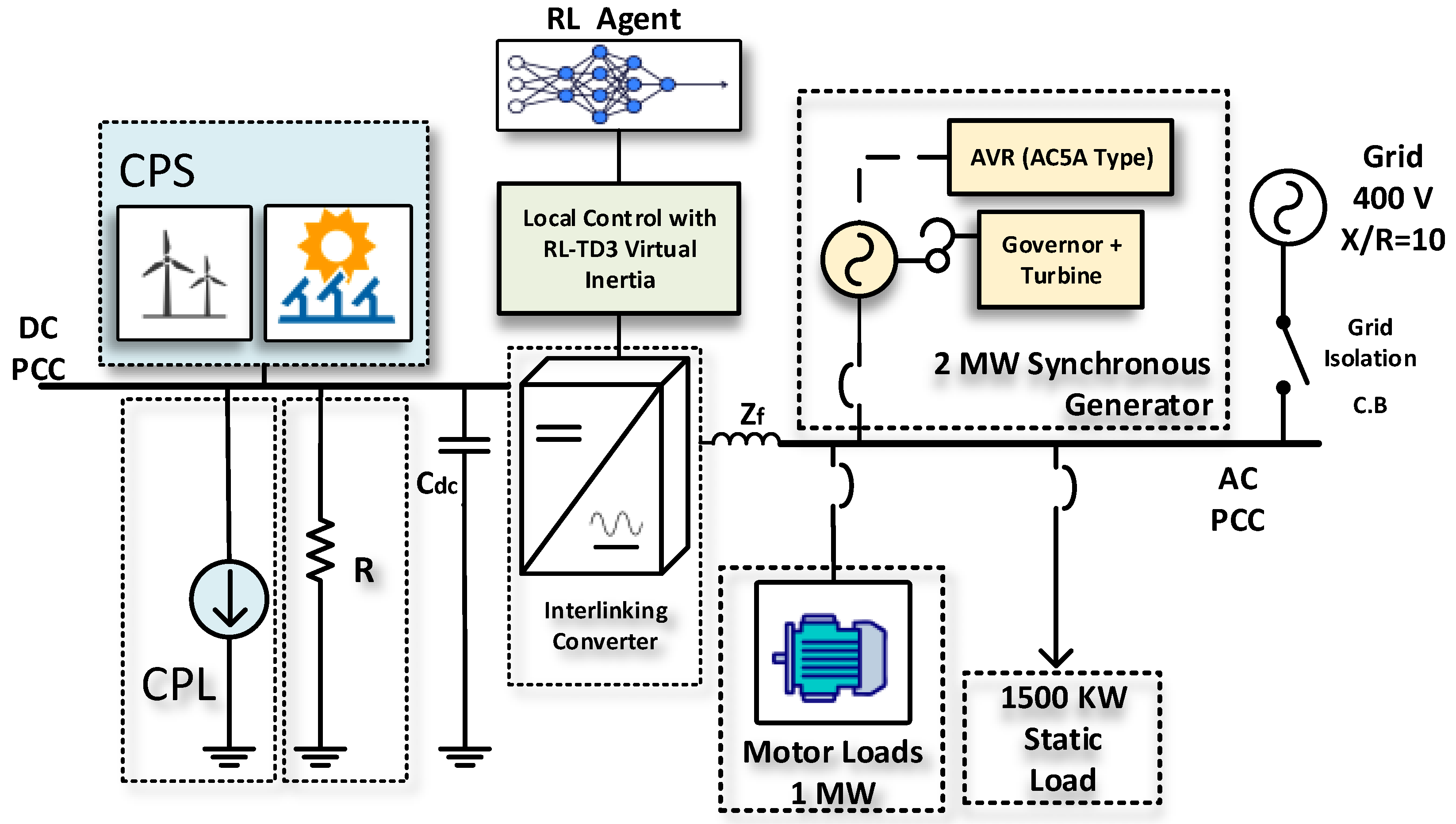
The microgrid system under study represents a common configuration used by oil and gas industries situated in remote areas far from the central power grid. The system also represents a typical power system when the grid is disconnected for a long time and only emergency supply and renewable energy sources are available. This microgrid predominantly relies on synchronous generators, including motor and static loads. In recent developments, the system has been augmented by integrating renewable energy sources. A prototypical site powered by synchronous generators utilizes droop control to distribute the load evenly. This setup serves as a model in the current study to simulate the dynamic operations characteristic of a standard oil and gas facility. Moreover, an adjacent DC microgrid, sourced from local renewable energy, has been implemented to support the AC grid loads.
Figure 1 illustrates the microgrid configuration being analyzed. This system comprises a diesel generator, various static loads, and induction motor loads. These components are all interconnected at the AC microgrid’s point of common coupling (PCC). Additionally, the DC microgrid is linked to the AC grid through a VSC, which is regulated by a virtual inertia control loop with the reinforcement learning agent based on the TD3 employed.
The DC microgrid consists of a constant power source representing renewable energy sources, such as a PV or wind system.
The system outlined in Figure 1 is the basis for analyzing the microgrid’s frequency response, focusing on the rate of change of frequency (RoCoF) and nadir. It also examines how AC-side fluctuations impact the DC microgrid’s DC voltage. Furthermore, the study delves into the dynamic efficacy of the suggested virtual inertia controller for frequency stabilization, as illustrated in the same figure.
For the purpose of the training process of the reinforcement learning agent, a small-signal linearized model of the microgrid’s components has been developed. The outcomes of this analysis are detailed in the subsequent subsections.
2.1. DC Microgrid Modeling
In this study, the VSC serves as the pivotal link between the DC and AC microgrids being examined. The control of the VSC plays a crucial role in maintaining the microgrid’s stability, especially during contingency scenarios. This is achieved by aiding the microgrid frequency in terms of the rate of change of frequency (RoCoF) and nadir through the provision of virtual inertia support. The VSC accomplishes this by adapting the reinforcement learning techniques.
The control system incorporates an agent trained in reinforcement learning, trained at reducing frequency deviations and improving nadir values. The study also includes a comparative analysis with two reinforcement learning agents, the DDPG and the TD3, to assess their effectiveness in mirroring dynamic behavior and enhancing overall performance. The subsequent sections will detail these different methods’ results and present a comparative analysis.
The net power contribution of the DC microgrid towards the AC grid, denoted as , is calculated by deducting the sum of the constant power load () and the resistive load present in the DC microgrid from the constant power source. Concurrently, the power transmission to the AC microgrid is represented by . Furthermore, the behavior of the DC link capacitor () associated with the interconnecting VSC is described by
Disregarding any losses in the VSC, Equation (2) delineates the power delivered to the AC microgrid.
where and represent the voltages in the DQ reference frame of the AC grid, and and represent the output currents of the VSC within the same DQ reference frame. In the DC microgrid, the renewable energy sources are effectively represented as a constant power source with a power output of . This constant power is consistently fed into the AC grid, and the voltage of the DC grid is controlled through the interlinking VSC. This mechanism is attributed to the relatively slow variation in power output from renewable energy sources, especially when compared to the dynamics of the inertia support loop. The resistive loads within the DC microgrid are modeled as resistance, denoted as R. As a result, the surplus power generated by the DC microgrid can be determined by the following calculation:
The linearized equation of the power transferred to the AC microgrid is given by (4):
where and are the base voltage and power of the system, and are the operating points where the system is linearized, and are small changes in the current in the DQ reference frame.
Figure 2 depicts the current control loop of the VSC, where the reference current values are denoted as and . In this setup, the q-reference is maintained at zero, whereas the d-reference is derived from the virtual inertia; the control includes an outer current loop and an inner voltage loop with the decoupling components. and represent the proportional–integral (PI) controller gains of the current loop. Notably, the virtual inertia loop is controlled by a reference signal provided by the agent’s actions, directly influencing the reference. The agent’s action is driven by the RL framework, where the states of the environment are measured through the frequency of the system and DC link voltage, and both are then compared to the nominal value to produce the errors as the states. The reward function drives the agent’s learning to generate the actions that produce the required virtual inertia support.
2.2. Model of Induction Machine
The dynamics of the induction motor (IM), particularly relations between its stator and rotor voltages and currents within the rotating reference frame, are listed in the equations denoted as (5). While these equations can be formulated using a variety of state variables, including both fluxes and currents, it is noted that these variables are not mutually exclusive. For the purpose of cohesively integrating the IM’s state equations into the broader linearized model of the microgrid, it is more advantageous to use currents as the state variables. Consequently, the interplay between stator and rotor voltage and current within the IM is detailed in the universally recognized synchronous DQ reference frame, as outlined in the following equations [44].
In these equations, and denote the inductances of the stator and rotor, respectively. Similarly, and refer to the resistances of the stator and rotor. Additionally, signifies the mutual inductance, refers to the synchronous speed, and indicates the speed of the rotor. The formulation of the electromagnetic torque within this context is presented as follows:
The correlation between torque and mechanical can be established:
where stands for the number of poles, J denotes the combined inertia of the motor and its load, and refers to the torque exerted by the load. It is important to note that before proceeding with the linearization of these machine equations, one must consider the influence of the stator supply frequency, which is governed by the droop equations in a microgrid system. This necessitates accounting for the minor variations in signal, essential for developing a comprehensive and integrated model for small-signal analysis. Therefore, the linear differential equations for the induction machine can be articulated as follows:
where is the state vector, is the input vector, is the system matrix, and is the input matrix, which is divided into two parts, and .
2.3. Model of Diesel Generator
2.3.1. Generator Model
The AC microgrid model utilized in this study incorporates a diesel generator, along with the dynamics of both the governor and the automatic voltage regulator (AVR). The synchronous generator within this model is defined such that represents the synchronous speed, and the difference between the actual rotor speed and this synchronous speed is expressed as .
The stator currents and voltages in the reference frame are denoted by and , respectively. Additionally, the stator fluxes in the frame are represented as . The rotor fluxes and input field voltage from the exciter are symbolized in their per-unit form as , and , respectively. stands for the mechanical power input from the turbine.
2.3.2. Governer and Engine Model
In this model, the governor and turbine are configured to endow the generator with a droop gain, designated as . This feature is critical for illustrating power distribution when multiple generators are in operation. Furthermore, the throttle actuator and the engine within the model are simulated using a low-pass filter approach. Each of these components is associated with its own time delay, identified as for the throttle actuator and for the engine, detailed as follows [45]:
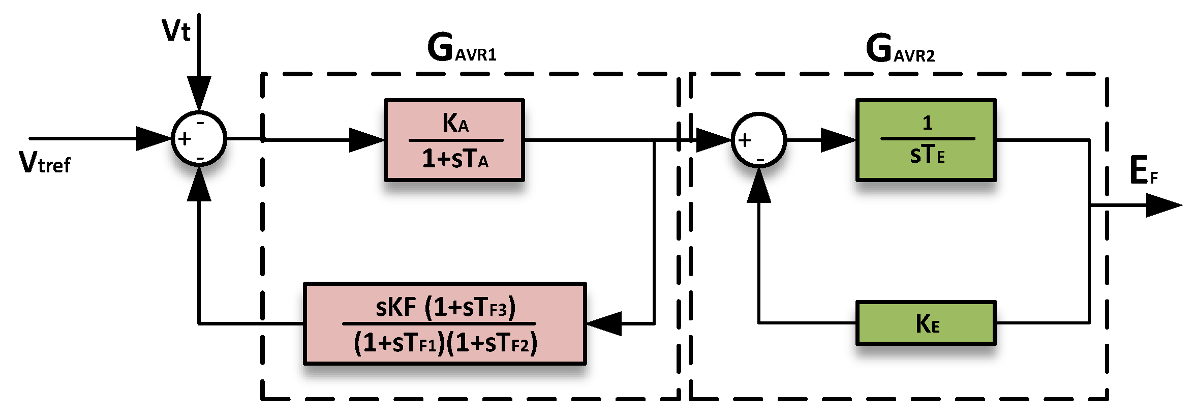
2.3.3. AVR Model
The AVR in the model is designed in line with the IEEE AC5A type, as illustrated in Figure 3. Key parameters of this AVR are shown in Table 2.
The AVR setup is determined as follows:
3. Reinforcement Learning Controller
The RL is a subset of machine learning, where an agent is trained to make optimal decisions through interactions with an environment guided by a system of states and rewards. This learning process involves the agent developing a policy, essentially a function that maps given states to actions, with the aim of maximizing cumulative rewards over time. The RL controller is utilized in this paper to be trained to provide frequency support by controlling the virtual inertia. In this context, the key components of an RL task are observation states, actions, and rewards, as shown in Figure 4.
In the system addressed in this study, the observation state and action are represented as and , respectively. They are defined as follows:
Such that represents the frequency deviation from its nominal value, and indicates the deviation in the DC link voltage. The integrated values of these errors are also included in the states. The action refers to the reference input for the (VSC) controller. The RL framework involves the RL agent interacting with a learning environment, in this case, the VSC controller. At each time step t, the environment provides the RL agent with a state observation . The RL controller then executes an action from its action space, observes the immediate reward , and updates the value of the state–action pair accordingly. This iterative process of exploration and refinement enables the RL-controlled controller to approximate an optimal control policy. The reward function is designed to penalize frequency deviation, DC link voltage deviation, and the magnitude of the previous action by the RL agent as follows:
such that is the absolute value of deviation in frequency from the nominal value, is the absolute DC link voltage deviation from the nominal value, and is the previous action by the RL agent; the values of the parameters used in the reward function are shown in Table 3.
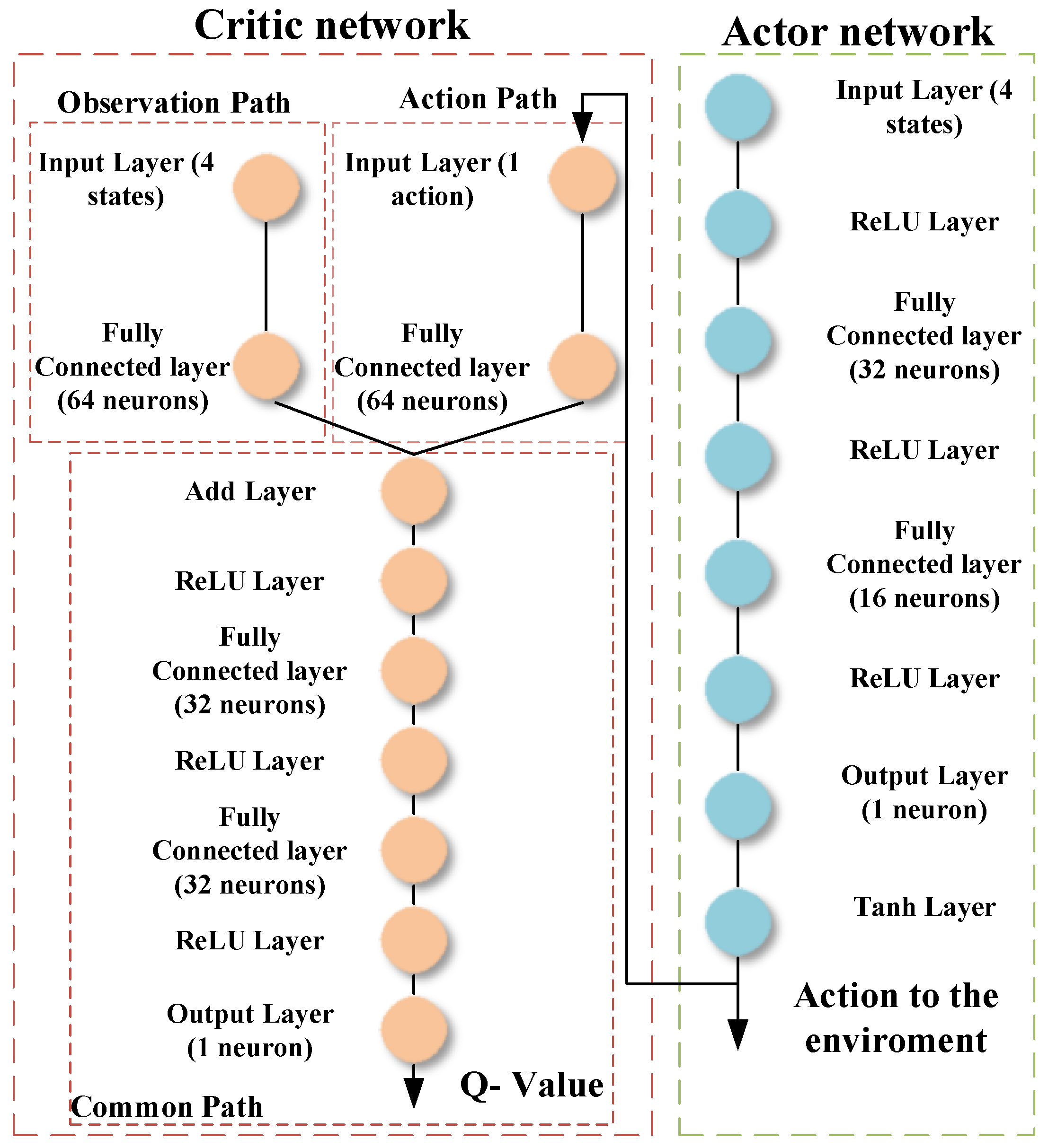
In this study, two RL agents are presented; the first agent is based on DDPG, presented and discussed in detail in [47], and the second agent is based on TD3. This section presents the structure and the training algorithm of the TD3 algorithm. The TD3 algorithm is an advanced model-free, online, off-policy reinforcement learning method, evolving from the DDPG algorithm. The TD3, designed to address DDPG’s tendency to overestimate value functions, incorporates key modifications for improved performance. It involves learning two Q-value functions and using the minimum of these estimates during policy updates, updating the policy and targets less frequently than Q functions, and adding noise to target actions during policy updates to avoid exploitation of actions with high Q-value estimates. The structure of the actor and critic networks used in this article is shown in Figure 5 and the structure of the DDPG actor and critic is shown in Figure 6.
The network architectures were designed using a comprehensive approach that balanced several considerations, including task complexity, computational resources, empirical methods, insights from the existing literature, and demands required by different network functions. Networks with more layers and neurons are needed in complex scenarios with high-dimensional state spaces and continuous action space. The methodology for selecting the most appropriate network architecture was mainly empirical, entailing the exploration and evaluation of various configurations. This iterative process typically begins with the deployment of relatively simple models, with subsequent adjustments involving incremental increases in complexity in response to training performance and computational time. The existing literature and benchmarks relevant to our task further informed our design choices. By examining successful network configurations applied to similar problems, we could draw upon established insights and best practices as a foundation for our architectural decisions. The activation function at the output neuron of the actor network greatly affected the network’s performance during the training; the tanh activation function fitted the most in the architecture of the actor network and produced the best outcome compared to the ReLU activation function.
During its training phase, a TD3 agent actively updates its actor and critic models at each time step, a process integral to its learning. It also employs a circular experience buffer to store past experiences, a crucial aspect of iterative learning. The agent utilizes mini-batches of these stored experiences to update the actor and critic, randomly sampled from the buffer. Furthermore, the TD3 agent introduces a unique aspect of perturbing the chosen action with stochastic noise at each training step, an approach that enhances exploration and learning efficacy.
The TD3 uses a combination of deterministic policy gradients and Q-learning to approximate the policy and value functions. The algorithm uses a deterministic actor function denoted by , where are its parameters, inputs the current state, and outputs deterministic actions to maximize long-term reward. The target actor function uses the same structure and parameterization as the actor function but with periodically updated parameters for stability. The TD3 also uses two Q-value critics , with parameters () to input observation () and action () and output the expected long-term reward. The critics have distinct parameters () and if two critics are used, they generally have the same structure but different initial parameters. The TD3 utilizes two target critics whose parameters () are periodically updated with the latest critic parameters. The actor, the target actor, the critics, and their respective targets have identical structures and parameterizations.
The actor network in a TD3 agent is trained by updating actor and critic properties at each time step during learning. It uses a circular experience buffer to store past experiences, sampling mini-batches from this buffer for updates. The action chosen by the policy is perturbed at each training step using stochastic noise. The actor is trained using a policy gradient. This gradient, , is approximated as follows:
with
where is the gradient of the minimum critic output with respect to the action, and is the gradient of the actor output with respect to the actor parameters, both evaluated for the observation . The actor parameters are then updated using the learning rate as follows:
In the TD3 algorithm, the critic is trained at each training step by minimizing the loss () for each critic network. The loss is calculated over a mini-batch of sampled experiences using the equation
where is the target value for the ith sample, is the output of the kth critic network for the state and action , and are the parameters of the kth critic network. This training process helps the critic to accurately estimate the expected rewards, contributing to the overall effectiveness of the TD3 algorithm. The critic parameters are then updated using the learning rate .
The target networks are then slowly updated using smoothing target factor .
The training algorithm of the TD3 agent is shown in Figure 7.
4. Simulation Results
This section evaluates the dynamic performance of the proposed RL-based virtual inertia controller for frequency support in the microgrid system presented in Section 2. The Matlab version used is 2022b alongside the Simulink and reinforcement learning toolbox. The computational features of the computer utilized are a dual-core processor of Intel Core i7 type, alongside 8 GB of RAM and a 500 GB SSD hard drive. The simulations are conducted in two separate steps. In the first step, the system is analyzed using a linearized model around an operating point where the synchronous generator supplies 0.75 pu, and the DC microgrid supplies 0.25 pu. This model is used for training the RL agent. This approach is adopted due to the intensive computational requirements and hardware resource utilization involved in training reinforcement learning agents and its difficulty in being implemented on a nonlinear model. The trained agents are applied to a nonlinear model to assess the dynamic response. The results obtained are compared with conventional methods, such as LPF and HPF controllers. A DDPG agent is also trained and examined to compare with the performance of the TD3 agent. This two-stage simulation comprehensively evaluates the system’s performance under different operational conditions.
4.1. Linear Model
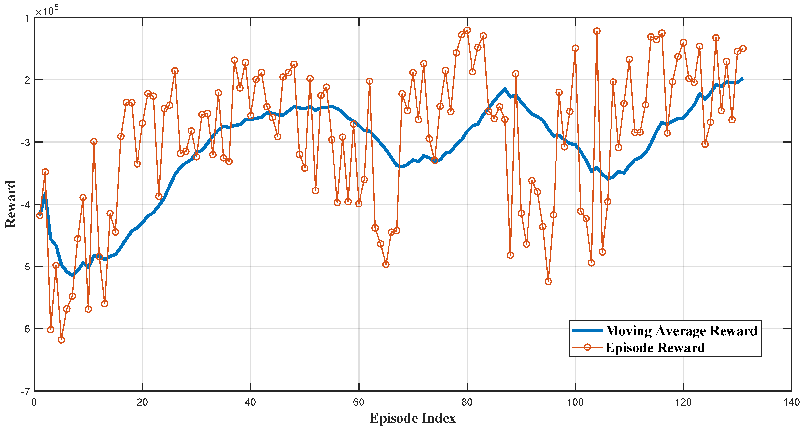
The RL agents in this study are trained in the linearized system environment, where the microgrid’s linearized model is considered the environment. During the training, the environment introduces a load disturbance in each training episode. Each training episode simulation time is s. The training process of the TD3 agent is visualized in Figure 8, plotting each episode’s reward along with the moving average value of the reward across the number of episodes equal to 20. This training continues until the moving average of the rewards meets the pre-determined criteria to stop training, ensuring the agent is adequately trained.
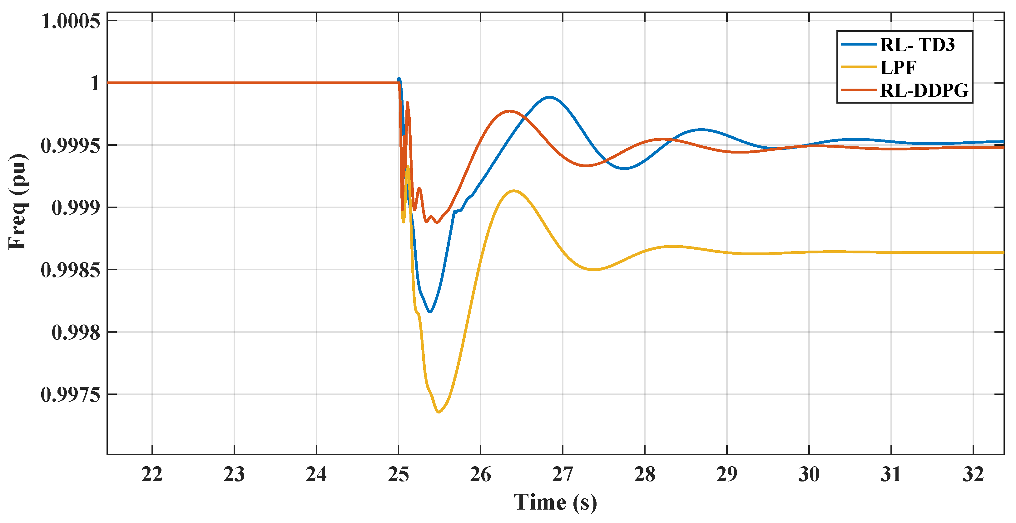
In the linearized system part of the simulation results, the comparative analysis of frequency responses to a dynamic load increase at s in the microgrid shown in Figure 1. Figure 9 shows distinct behaviors among the different control methodologies: RL-TD3, RL-DDPG, LPF, and HPF. The reinforcement-learning-based TD3 controller (RL-TD3) and the DDPG controller exhibit a rapid recovery from the disturbance, achieving a superior rate of frequency change and maintaining a nadir point closer to the nominal value than other techniques with higher performance of the DDPG. On the other hand, the LPF controller shows a moderate response with a more noticeable deviation. The HPF controller, in contrast, experiences the most significant frequency dip and the slowest recovery. This comparison underscores the effectiveness of the RL agents in maintaining frequency stability under dynamic load conditions, surpassing the performance of LPF and HPF controllers. It is important to note that the DDPG-RL agent was also trained on the same linear system as the TD3 agent in the simulation. However, it required significantly more training time, taking 280 episodes to reach the designated average reward threshold, compared to only 131 episodes for the TD3 agent.
Figure 10 illustrates the DC voltage responses for the same case of a 3% dynamic load increase for the different controllers. The RL-DDPG controller initially shows a sharp voltage drop, indicating strong inertial support to the AC microgrid, but it successfully keeps the DC link voltage within a 5% change boundary. It reaches its nadir earlier than the other controllers, providing the best inertial support due to the power transfer to the AC grid before stabilizing. It is followed by the RL-TD3 agent, which encounters similar behavior in voltage drop but tries to restore the voltage to reduce the penalty or increase the reward when the frequency deviation starts to decrease; however, when the frequency deviation starts to grow back again, the agent drops the voltage to the maximum level to reduce the frequency deviation through inertial support. In comparison, LPF exhibits moderate dips with oscillatory tendencies, while HPF maintains a relatively stable voltage profile. Overall, the RL controllers demonstrate robust transient response and effective inertial support, outperforming conventional controllers in maintaining voltage stability under dynamic load conditions.
The controller’s stability in the linearized system was tested in the study by examining the controller’s response under different loading conditions. This approach was aimed at assessing the controller’s robustness under varying conditions. The performance and stability of the controller were then compared with that of the low-pass filter (LPF) controller. This comparison was crucial to evaluate how well each controller adapted to changes in the system’s dynamics and maintained operational stability, providing valuable insights into the effectiveness of the proposed control strategy under different scenarios.
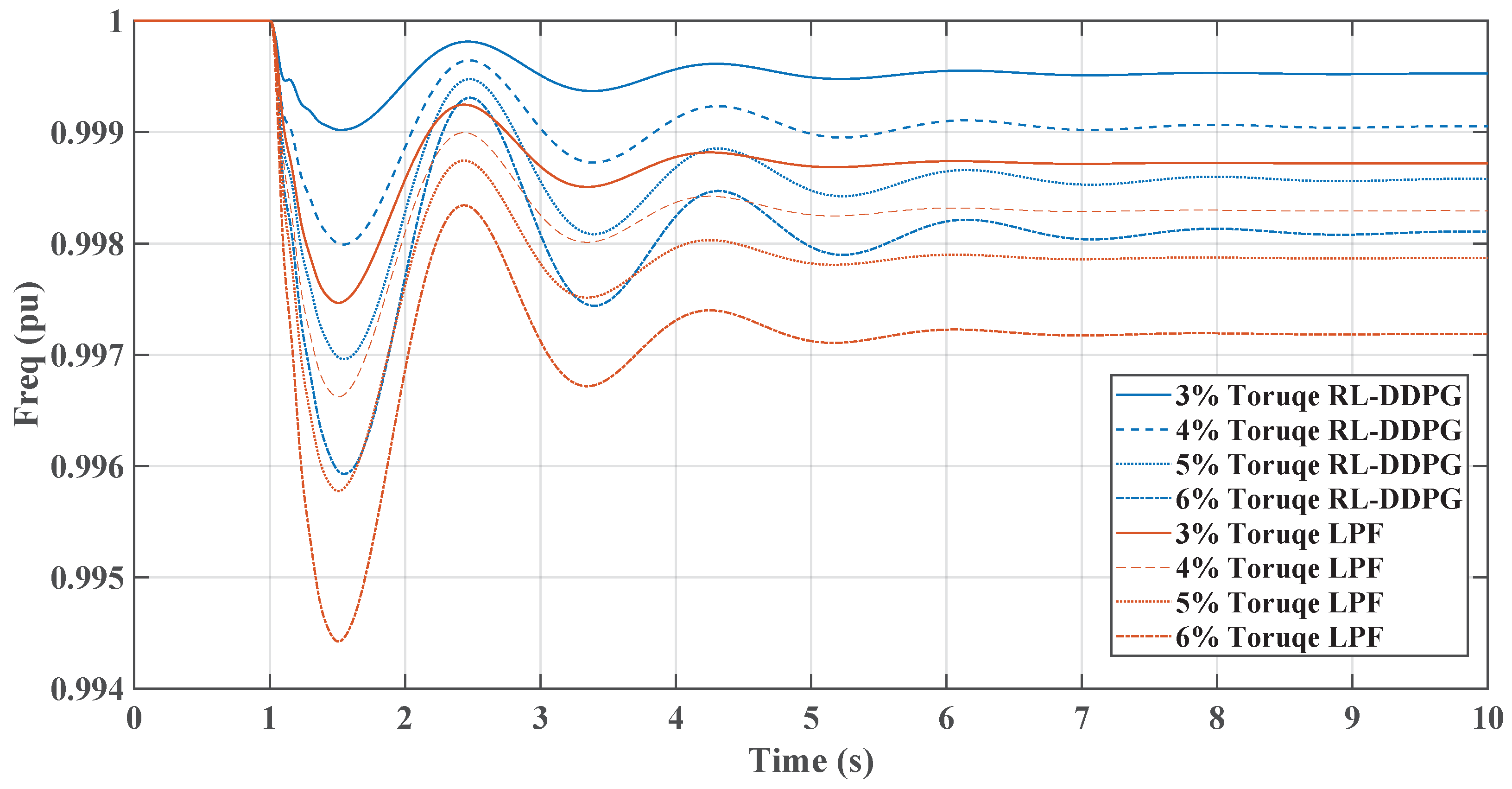
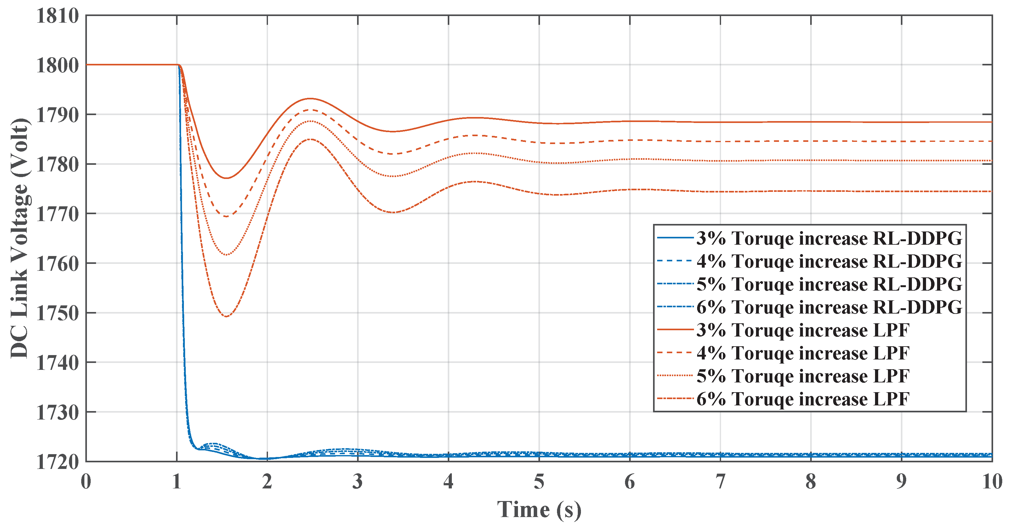
Figure 11, comparing the RL-TD3 and LPF controllers under dynamic torque load increases from 3% to 6%, shows the RL controller’s superior performance in managing disturbances. Both controllers exhibit oscillatory behaviors post-disturbance, but the RL controller stabilizes in less setting time to the nominal frequency, particularly at higher torque loads. The RL controller’s frequency nadir values are less pronounced than those of the LPF, indicating a more robust response. On the other hand, in Figure 12, the LPF controller shows larger oscillations and a slower return to baseline. Under these conditions, the DC link voltage response graph reveals the RL controller’s more pronounced voltage drop, signifying greater power allocation to the AC side for enhanced inertial support, especially critical during substantial load changes. In contrast, the LPF maintains higher DC voltage levels but may offer different inertial support levels. The RL controller’s approach is beneficial for grid stability in microgrids, provided the voltage remains within the boundaries. The same change in load torque is made, and the response for the RL-DDPG controller compared to the LPF is shown in Figure 13 and Figure 14, which show a superior performance of the RL-DDPG over the conventional LPF controller.
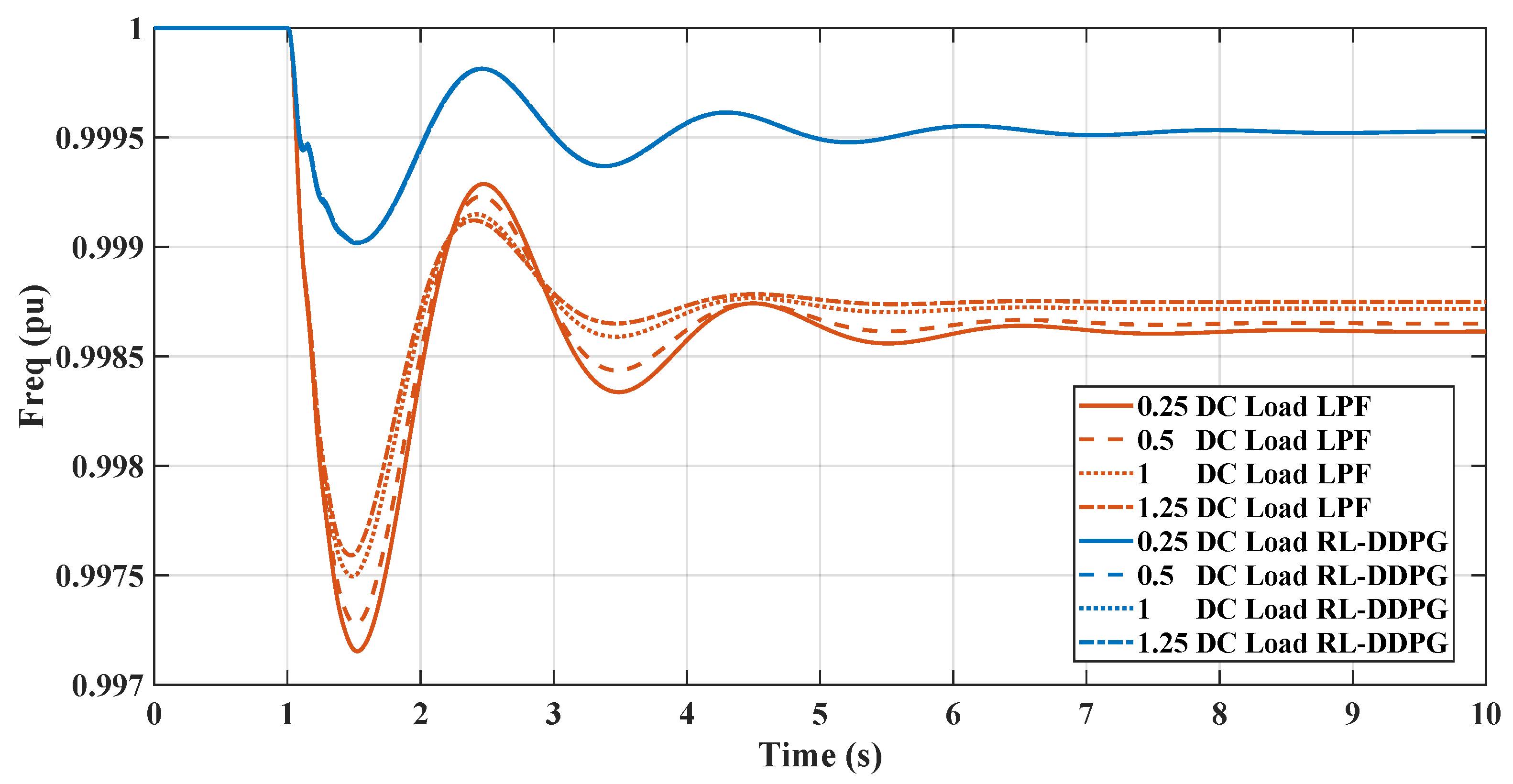
Figure 15 and Figure 16 demonstrate the impact of varying static load levels on the microgrid’s frequency regulation performance, specifically when managed by RL and LPF controllers. With increased static load, from pu to pu, both the RL controllers adeptly handle the additional demand, maintaining frequency stability with minimal deviation. This indicates the RL controller’s robustness and ability to provide effective inertial support even as static load parameters change, reflecting a resilient control strategy suitable for dynamic microgrid environments.
4.2. Nonlinear Model
Following the successful implementation and validation of a linearized model, the RL controllers are then integrated into a nonlinear model to evaluate its robustness. This crucial step ensures that each controller’s performance holds under more complex and realistic operating conditions. Examining each controller’s behavior in a nonlinear environment is fundamental to validating its efficacy, providing a comprehensive understanding of its potential in practical applications. This further confirms the controllers’ capabilities, reinforcing confidence in its deployment for real-world microgrid applications.
In the nonlinear model environment, the RL controllers’ frequency and DC voltage responses to a 3% increase in dynamic load at are depicted in Figure 17 and Figure 18. The frequency response demonstrates a similar pattern to that observed in the linearized model, with the controller effectively dampening oscillations and rapidly returning to the nominal frequency after a disturbance. The DC voltage response also performs similarly to the linearized environment, displaying a sharp initial drop and then stabilizing without exceeding the 5% boundaries, illustrating the controllers’ robustness. This consistent behavior across linear and nonlinear models underscores the RL controllers’ reliability and effectiveness in dynamic conditions.
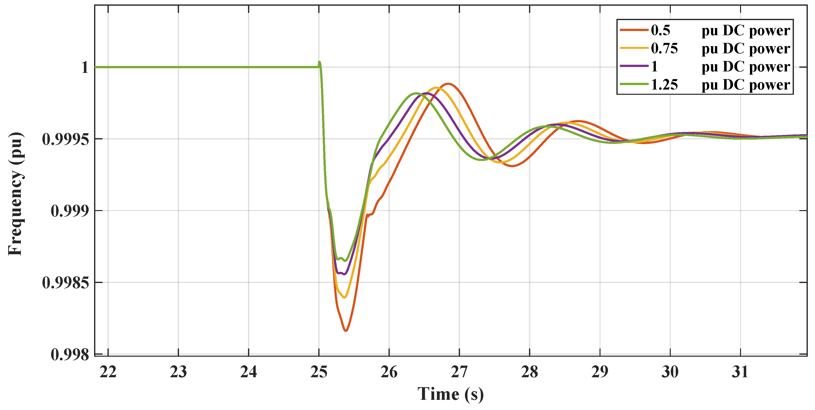
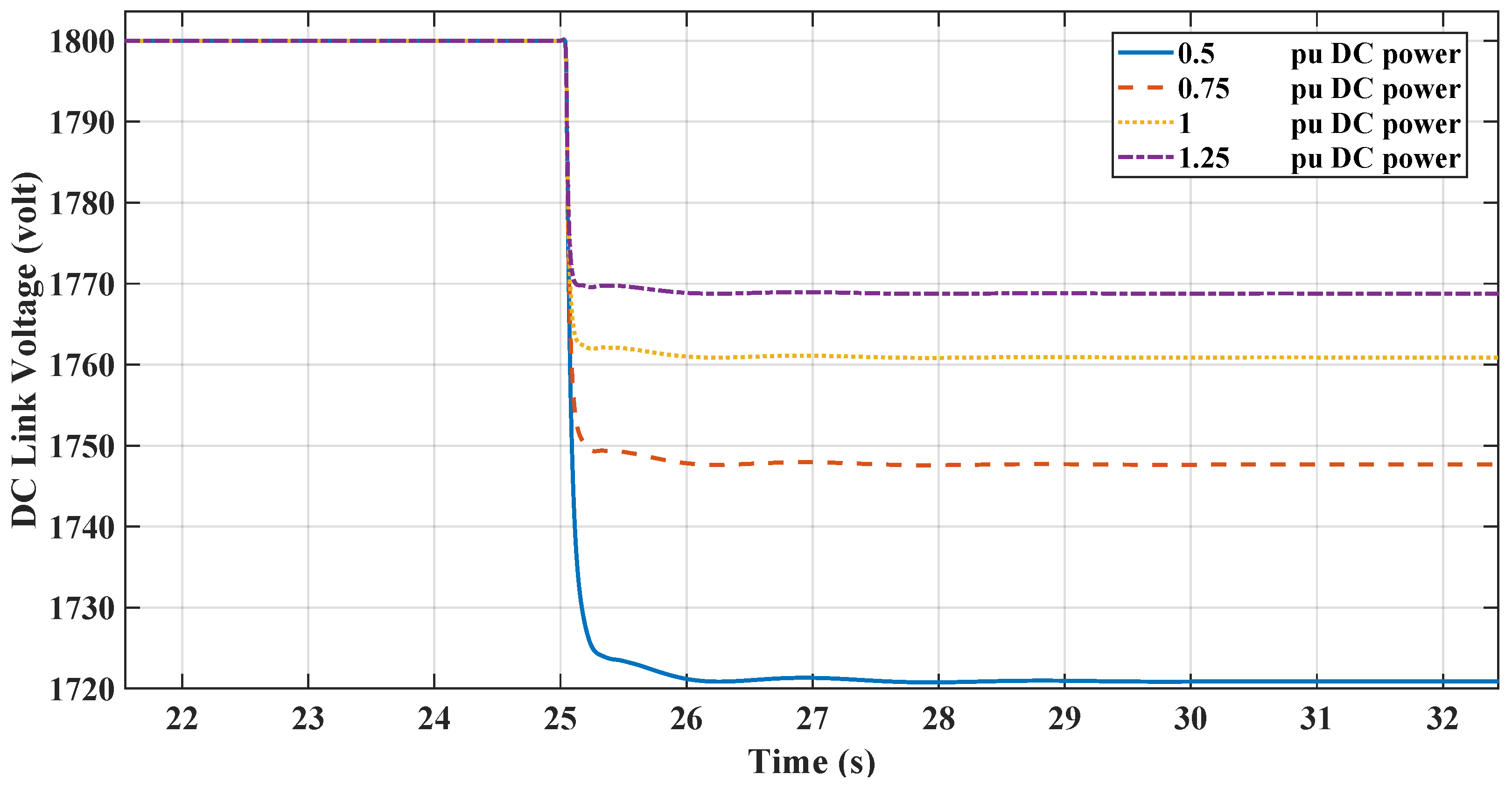
This section illustrates the robust performance of the RL controllers in a nonlinear microgrid environment. The graph in Figure 19 demonstrates the frequency response under varying DC loads, where the TD3 controller maintains frequency stability despite DC load variations. Figure 20 shows the DC link voltage response, indicating that the controller adeptly manages voltage sags, contributing to effective inertial support. The graph in Figure 21 demonstrates the frequency response under varying DC loads, where the DDPG controller maintains frequency stability despite DC load variations. Figure 22 shows the DC link voltage response; both figures indicate that the controllers have a similar response to the linear model.
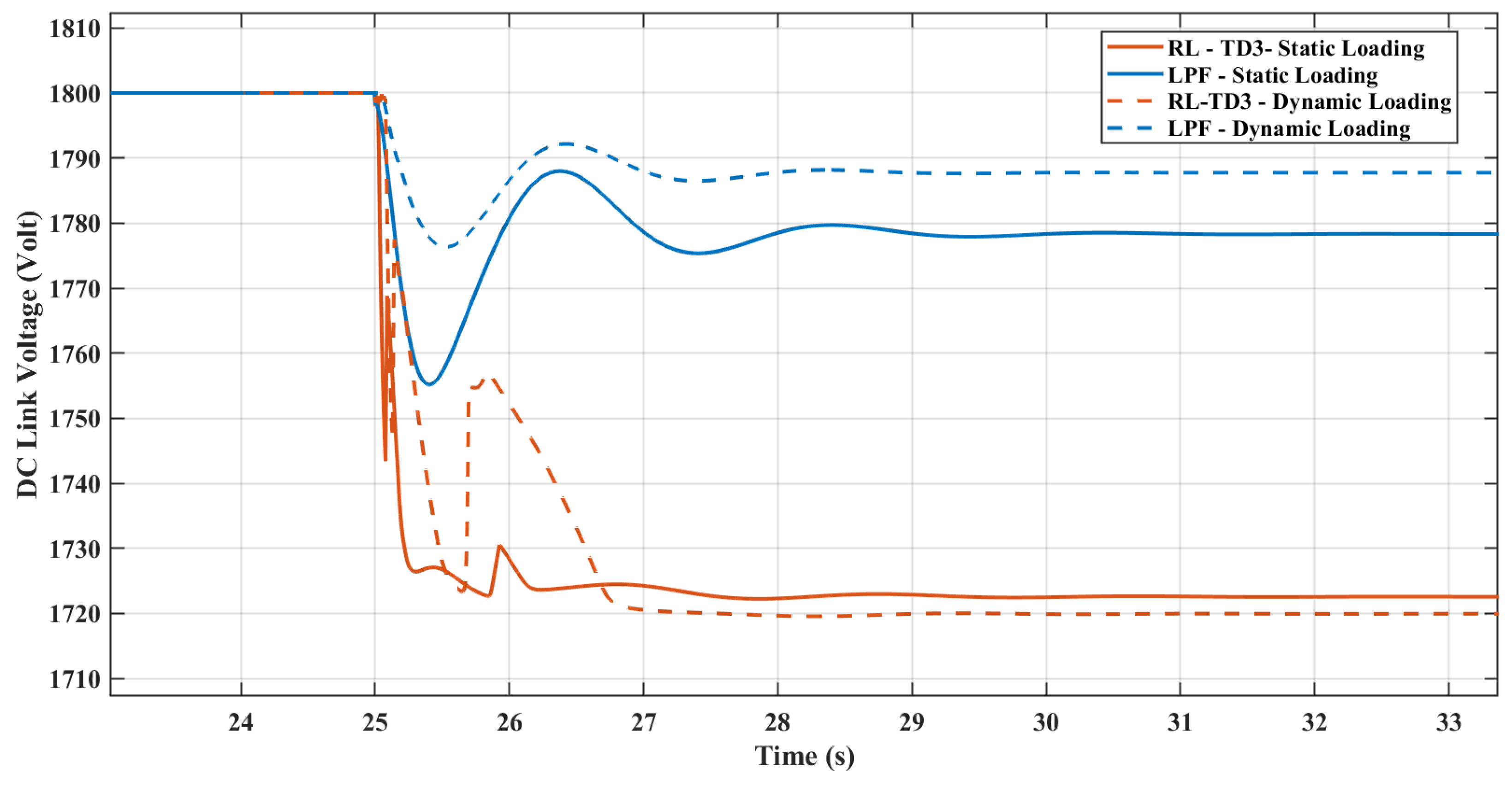
Figure 23 depicts the frequency response of decreasing the microgrid’s overall inertia by turning off the dynamic loading and replacing the induction motor with an equal amount of power of static loading. The results show the comparison between the response of the proposed RL controller compared with the conventional LPF controller. The RL controller depicts a better inertial response regarding RoCoF and nadir than the conventional controller. The figure also contains the same comparison when the loading utilized is a dynamic load; the frequency nadir in both controllers’ cases is lower in the case of dynamic loading. The results show the effect of reducing overall inertia due to the replacement of induction machine loads and demonstrate the robustness of the proposed RL controller.
Figure 24 depicts the DC link voltage for replacing the dynamic loads with static loads. The DC link voltage demonstrates that the RL agent is trained to transfer the maximum allowed inertia support to the AC microgrid by reducing the DC link voltage.
5. Conclusions
This paper presented a new control algorithm that utilizes the Twin Delayed Deep Deterministic Policy Gradient (TD3) and Deep Deterministic Policy Gradient (DDPG) reinforcement learning methods to support the frequency in low-inertia grids. The RL agents are trained using the system-linearized model and then extended to the nonlinear model to reduce the computational burden. The Matlab/Simulink and reinforcement learning toolbox are utilized to compare the system performance using the proposed AI-based methods with conventional low-pass and high-pass filter (LPF and HPF) controllers referenced in the literature. The proposed TD3- and DDPG-based frequency support controllers demonstrate superior performance over the conventional methods, where the frequency dynamics in terms of RoCoF and nadir are significantly improved. The inertial support provided to the AC microgrid site is sourced from the DC microgrid side’s DC link voltage. At different loading scenarios based on the nonlinear model under various operating conditions, the results show the robustness of the proposed algorithms against various disturbances. The conducted work emphasizes the pivotal role of reinforcement learning in enhancing the dynamic performance of low-inertia grids, which facilitates the integration of more renewable energy resources into existing grids. The controller poses some limitations due to the complexity of the neural networks, which results in complexity in studying the stability analysis and needs a high processing time during the training and testing of the proposed controller. Future work will include fault analysis of the proposed microgrid system and testing the proposed controller’s response to faults.
Author Contributions
Conceptualization, A.M.I.M. and M.I.M.; methodology, A.M.I.M. and M.I.M.; software, A.M.I.M. and M.A.A.; validation, A.M.I.M. and M.A.A.; formal analysis, A.M.I.M. and M.A.A.; investigation, A.M.I.M., M.A.A. and M.I.M.; resources, A.M.I.M. and M.I.M.; data curation, A.M.I.M. and M.A.A.; writing-original draft preparation, M.A.A. and A.M.I.M.; writing-review and editing, A.M.I.M. and M.I.M.; visualization, A.M.I.M. and M.A.A.; supervision, A.M.I.M. and M.I.M.; project administration, A.M.I.M. and M.I.M.; funding acquisition, M.I.M. All authors have read and agreed to the published version of the manuscript.
Funding
This research received no external funding.
Institutional Review Board Statement
Not applicable.
Informed Consent Statement
Not applicable.
Data Availability Statement
The original contributions presented in the study are included in the article, further inquiries can be directed to the corresponding author.
Conflicts of Interest
The authors declare no conflicts of interest.
Abbreviations
The following abbreviations are used in this manuscript:
| AVR | Automatic voltage regulator |
| CPS | Constant power source |
| DDPG | Deep Deterministic Policy Gradient |
| DERs | Distributed energy resources |
| DQN | Deep Q-Networks |
| HPF | High-pass filter |
| IM | Induction motor |
| LPF | Low-pass filter |
| MG | Microgrid |
| PCC | Point of common coupling |
| PEL | Power electronics-linked |
| PI | Proportional–integral |
| PV | Photovoltaic |
| RESs | Renewable energy sources |
| RL | Reinforcement learning |
| RoCoF | Rate of change of frequency |
| SGs | Synchronous generators |
| TD3 | Twin Delayed Deep Deterministic Policy Gradient |
| VI | Virtual inertia |
| VSCs | Voltage source converters |
| VSGs | Virtual synchronous generators |
| VSMs | Virtual synchronous machines |
References
- Qadir, S.; Al-Motairi, H.; Tahir, F.; Al-Fagih, L. Incentives and strategies for financing the renewable energy transition: A review. Energy Rep. 2021, 7, 3590–3606. [Google Scholar] [CrossRef]
- Kabeyi, M.; Olanrewaju, O. Sustainable Energy Transition for Renewable and Low Carbon Grid Electricity Generation and Supply. Front. Energy Res. 2022, 9, 43114. [Google Scholar] [CrossRef]
- Genc, T.; Kosempel, S. Energy Transition and the Economy: A Review Article. Energies 2023, 16, 2965. [Google Scholar] [CrossRef]
- Osman, A.; Chen, L.; Yang, M.; Msigwa, G.; Farghali, M.; Fawzy, S.; Rooney, D.; Yap, P. Cost, environmental impact, and resilience of renewable energy under a changing climate: A review. Environ. Chem. Lett. 2023, 21, 741–764. [Google Scholar] [CrossRef]
- Stram, B. Key challenges to expanding renewable energy. Energy Policy 2016, 96, 728–734. [Google Scholar] [CrossRef]
- Denholm, P.; Mai, T.; Kenyon, R.; Kroposki, B.; O’Malley, M. Inertia and the Power Grid: A Guide without the Spin; National Renewable Energy Lab (NREL): Golden, CO, USA, 2020.
- Khazaei, J.; Tu, Z.; Liu, W. Small-Signal Modeling and Analysis of Virtual Inertia-Based PV Systems. IEEE Trans. Energy Convers. 2020, 35, 1129–1138. [Google Scholar] [CrossRef]
- Soni, N.; Doolla, S.; Chandorkar, M. Improvement of Transient Response in Microgrids Using Virtual Inertia. IEEE Trans. Power Deliv. 2013, 28, 1830–1838. [Google Scholar] [CrossRef]
- Bakhshi-Jafarabadi, R.; Lekić, A.; Marvasti, F.; Jesus, C.J.; Popov, M. Analytical Overvoltage and Power-Sharing Control Method for Photovoltaic-Based Low-Voltage Islanded Microgrid. IEEE Access 2023, 11, 134286–134297. [Google Scholar] [CrossRef]
- Guerrero, J.; Vasquez, J.; Matas, J.; Vicuna, L.; Castilla, M. Hierarchical Control of Droop-Controlled AC and DC Microgrids—A General Approach Toward Standardization. IEEE Trans. Ind. Electron. 2011, 58, 158–172. [Google Scholar] [CrossRef]
- Mohamed, S.; Mokhtar, M.; Marei, M. An adaptive control of remote hybrid microgrid based on the CMPN algorithm. Electr. Power Syst. Res. 2022, 213, 108793. [Google Scholar] [CrossRef]
- Guerrero, J.; Loh, P.; Lee, T.; Chandorkar, M. Advanced Control Architectures for Intelligent Microgrids—Part II: Power Quality, Energy Storage, and AC/DC Microgrids. IEEE Trans. Ind. Electron. 2013, 60, 1263–1270. [Google Scholar] [CrossRef]
- Nair, D.; Nair, M.; Thakur, T. A Smart Microgrid System with Artificial Intelligence for Power-Sharing and Power Quality Improvement. Energies 2022, 15, 5409. [Google Scholar] [CrossRef]
- EL-Ebiary, A.; Mokhtar, M.; Mansour, A.; Awad, F.; Marei, M.; Attia, M. Distributed Mitigation Layers for Voltages and Currents Cyber-Attacks on DC Microgrids Interfacing Converters. Energies 2022, 15, 9426. [Google Scholar] [CrossRef]
- González, I.; Calderón, A.; Folgado, F. IoT real time system for monitoring lithium-ion battery long-term operation in microgrids. J. Energy Storage 2022, 51, 104596. [Google Scholar] [CrossRef]
- Zhang, Z.; Dou, C.; Yue, D.; Zhang, Y.; Zhang, B.; Zhang, Z. Event-Triggered Hybrid Voltage Regulation with Required BESS Sizing in High-PV-Penetration Networks. IEEE Trans. Smart Grid 2022, 13, 2614–2626. [Google Scholar] [CrossRef]
- Nassif, A.; Ericson, S.; Abbey, C.; Jeffers, R.; Hotchkiss, E.; Bahramirad, S. Valuing Resilience Benefits of Microgrids for an Interconnected Island Distribution System. Electronics 2022, 11, 4206. [Google Scholar] [CrossRef]
- Abdulmohsen, A.; Omran, W. Active/reactive power management in islanded microgrids via multi-agent systems. Int. J. Electr. Power Energy Syst. 2022, 135, 107551. [Google Scholar] [CrossRef]
- Ortiz-Villalba, D.; Rahmann, C.; Alvarez, R.; Canizares, C.; Strunck, C. Practical Framework for Frequency Stability Studies in Power Systems With Renewable Energy Sources. IEEE Access 2020, 8, 202286–202297. [Google Scholar] [CrossRef]
- Anwar, M.; Marei, M.; El-Sattar, A. Generalized droop-based control for an islanded microgrid. In Proceedings of the 2017 12th International Conference on Computer Engineering And Systems (ICCES), Cairo, Egypt, 19–20 December 2017; pp. 717–722. [Google Scholar]
- Fallah, F.; Ramezani, A.; Mehrizi-Sani, A. Integrated Fault Diagnosis and Control Design for DER Inverters using Machine Learning Methods. In Proceedings of the 2022 IEEE Power & Energy Society General Meeting (PESGM), Denver, CO, USA, 17–21 July 2022; pp. 1–5. [Google Scholar]
- Al Hassan, H.; Alharbi, T.; Morello, S.; Mao, Z.; Grainger, B. Linear Quadratic Integral Voltage Control of Islanded AC Microgrid Under Large Load Changes. In Proceedings of the 2018 9th IEEE International Symposium on Power Electronics for Distributed Generation Systems (PEDG), Charlotte, NC, USA, 25–28 June 2018; pp. 1–5. [Google Scholar]
- Rocabert, J.; Luna, A.; Blaabjerg, F.; Rodríguez, P. Control of Power Converters in AC Microgrids. IEEE Trans. Power Electron. 2012, 27, 4734–4749. [Google Scholar] [CrossRef]
- Li, Z.; Chan, K.; Hu, J.; Guerrero, J. Adaptive Droop Control Using Adaptive Virtual Impedance for Microgrids With Variable PV Outputs and Load Demands. IEEE Trans. Ind. Electron. 2021, 68, 9630–9640. [Google Scholar] [CrossRef]
- Li, Y.; Tang, F.; Wei, X.; Qin, F.; Zhang, T. An Adaptive Droop Control Scheme Based on Sliding Mode Control for Parallel Buck Converters in Low-Voltage DC Microgrids. In Proceedings of the 2021 IEEE 4th International Electrical and Energy Conference (CIEEC), Wuhan, China, 28–30 May 2021; pp. 1–6. [Google Scholar]
- Zhang, L.; Chen, K.; Lyu, L.; Cai, G. Research on the Operation Control Strategy of a Low-Voltage Direct Current Microgrid Based on a Disturbance Observer and Neural Network Adaptive Control Algorithm. Energies 2019, 12, 1162. [Google Scholar] [CrossRef]
- Yang, X.; Wang, Y.; Zhang, Y.; Xu, D. Modeling and Analysis of Communication Network in Smart Microgrids. In Proceedings of the 2018 2nd IEEE Conference on Energy Internet and Energy System Integration (EI2), Beijing, China, 20–22 October 2018; pp. 1–6. [Google Scholar]
- Hu, J.; Shan, Y.; Cheng, K.; Islam, S. Overview of power converter control in microgrids—Challenges, advances, and future trends. IEEE Trans. Power Electron. 2022, 37, 9907–9922. [Google Scholar] [CrossRef]
- Alhelou, H.; Golshan, M.; Njenda, T.; Hatziargyriou, N. An overview of UFLS in conventional, modern, and future smart power systems: Challenges and opportunities. Electr. Power Syst. Res. 2020, 179, 106054. [Google Scholar] [CrossRef]
- Afifi, M.; Marei, M.; Mohamad, A. Modelling, Analysis and Performance of a Low Inertia AC-DC Microgrid. Appl. Sci. 2023, 13, 3197. [Google Scholar] [CrossRef]
- Beck, H.; Hesse, R. Virtual synchronous machine. In Proceedings of the 2007 9th International Conference on Electrical Power Quality and Utilisation, Barcelona, Spain, 9–11 October 2007; pp. 1–6. [Google Scholar]
- Driesen, J.; Visscher, K. Virtual synchronous generators. In Proceedings of the 2008 IEEE Power and Energy Society General Meeting-Conversion and Delivery of Electrical Energy in the 21st Century, Pittsburgh, PA, USA, 20–24 July 2008; pp. 1–3. [Google Scholar]
- Chen, M.; Zhou, D.; Blaabjerg, F. Modelling, implementation, and assessment of virtual synchronous generator in power systems. J. Mod. Power Syst. Clean Energy 2020, 8, 399–411. [Google Scholar] [CrossRef]
- Tamrakar, U.; Shrestha, D.; Maharjan, M.; Bhattarai, B.; Hansen, T.; Tonkoski, R. Virtual inertia: Current trends and future directions. Appl. Sci. 2017, 7, 654. [Google Scholar] [CrossRef]
- Vetoshkin, L.; Müller, Z. A comparative analysis of a power system stability with virtual inertia. Energies 2021, 14, 3277. [Google Scholar] [CrossRef]
- Zhao, S.; Blaabjerg, F.; Wang, H. An Overview of Artificial Intelligence Applications for Power Electronics. IEEE Trans. Power Electron. 2021, 36, 4633–4658. [Google Scholar] [CrossRef]
- Skiparev, V.; Belikov, J.; Petlenkov, E. Reinforcement learning based approach for virtual inertia control in microgrids with renewable energy sources. In Proceedings of the 2020 IEEE PES Innovative Smart Grid Technologies Europe (ISGT-Europe), The Hague, The Netherlands, 26–28 October 2020; pp. 1020–1024. [Google Scholar]
- Fujimoto, S.; Hoof, H.; Meger, D. Addressing function approximation error in actor-critic methods. In Proceedings of the International Conference on Machine Learning, Stockholm, Sweden, 10–15 July 2018; pp. 1587–1596. [Google Scholar]
- Egbomwan, O.; Liu, S.; Chaoui, H. Twin Delayed Deep Deterministic Policy Gradient (TD3) Based Virtual Inertia Control for Inverter-Interfacing DGs in Microgrids. IEEE Syst. J. 2022, 17, 2122–2132. [Google Scholar] [CrossRef]
- Skiparev, V.; Nosrati, K.; Tepljakov, A.; Petlenkov, E.; Levron, Y.; Belikov, J.; Guerrero, J. Virtual Inertia Control of Isolated Microgrids Using an NN-Based VFOPID Controller. IEEE Trans. Sustain. Energy 2023, 14, 1558–1568. [Google Scholar] [CrossRef]
- Skiparev, V.; Nosrati, K.; Petlenkov, E.; Belikov, J. Reinforcement Learning Based Virtual Inertia Control of Multi-Area Microgrids; Elsevier: Amsterdam, The Netherlands, 2023. [Google Scholar] [CrossRef]
- Barbalho, P.; Lacerda, V.; Fernandes, R.; Coury, D. Deep reinforcement learning-based secondary control for microgrids in islanded mode. Electr. Power Syst. Res. 2022, 212, 108315. [Google Scholar] [CrossRef]
- Yi, Z.; Xu, Y.; Wang, X.; Gu, W.; Sun, H.; Wu, Q.; Wu, C. An Improved Two-Stage Deep Reinforcement Learning Approach for Regulation Service Disaggregation in a Virtual Power Plant. IEEE Trans. Smart Grid 2022, 13, 2844–2858. [Google Scholar] [CrossRef]
- Mohamad, A.M.; Arani, M.F.M.; Mohamed, Y.A.R.I. Investigation of Impacts of Wind Source Dynamics and Stability Options in DC Power Systems With Wind Energy Conversion Systems. IEEE Access 2020, 8, 18270–18283. [Google Scholar] [CrossRef]
- Kundur, P. Power System Stability and Control; McGraw-Hill Professional: New York, NY, USA, 1994. [Google Scholar]
- Sauer, P.; Pai, M. Power System Dynamics and Stability; Pearson: London, UK, 1997. [Google Scholar]
- Afifi, M.; Marei, M.; Mohamad, A. Reinforcement Learning Approach with Deep Deterministic Policy Gradient DDPG-Controlled Virtual Synchronous Generator for an Islanded Microgrid. In Proceedings of the 2023 24th International Middle East Power Systems Conference (MEPCON), Mansoura, Egypt, 19 December 2023. [Google Scholar]
Figure 1.
Microgrid system under study.

Figure 2.
Control of the VSC in the RL framework.

Figure 3.
AVR model.

Figure 4.
Reinforcement learning framework.

Figure 5.
Structure of the actor and critic networks for the RL-TD3 agent.

Figure 6.
Structure of the actor and critic networks for the RL-DDPG agent.

Figure 7.
TD3 training algorithm.

Figure 8.
Cumulative reward for each training episode.

Figure 9.
Comparison between RL-TD3, RL-DDPG, LPF-, and HPF-based controllers for virtual inertia loop in terms of frequency response.
Figure 9.
Comparison between RL-TD3, RL-DDPG, LPF-, and HPF-based controllers for virtual inertia loop in terms of frequency response.

Figure 10.
Comparison between RLTD3, RL-DDPG, LPF-, and HPF-based controllers for virtual inertia loop in terms of DC link voltage.
Figure 10.
Comparison between RLTD3, RL-DDPG, LPF-, and HPF-based controllers for virtual inertia loop in terms of DC link voltage.

Figure 11.
TD3-RL and LPF frequency response under dynamic load increase.

Figure 12.
TD3-RL and LPF DC voltage response under dynamic load increase.

Figure 13.
RL-DDPG and LPF frequency response under dynamic load increase.

Figure 14.
RL-DDPG and LPF DC voltage response under dynamic load increase.

Figure 15.
RL-TD3 and LPF frequency response under DC static load change.

Figure 16.
RL-DDPG and LPF frequency response under DC static load change.

Figure 17.
TD3-RL frequency response in nonlinear model.

Figure 18.
TD3-RL DC voltage response in nonlinear model.

Figure 19.
RL-TD3 frequency response with changing DC loading.

Figure 20.
RL-TD3 DC voltage response with changing DC loading.

Figure 21.
RL-DDPG frequency response with changing DC loading.

Figure 22.
RL-DDPG DC voltage response with changing DC loading.

Figure 23.
Frequency response with replacing the dynamic loading with static loading.

Figure 24.
DC link voltage response with replacing the dynamic loading with static loading.


Table 1.
Parameters of the synchronous generator.
| Parameter | Value (pu) | Parameter | Value (pu) |
|---|---|---|---|
| H | 1.5 | D | 1.33 |
| 0.0095 | 2.11 | ||
| 0.17 | 0.13 | ||
| 1.56 | 1.56 | ||
| 0.23 | 0.05 | ||
| 4.4849 | 0.0681 | ||
| 0.33 × 0.00001 | 0.1 |
Table 2.
The values of parameters of the AVR.
| Parameter | Name | Value |
|---|---|---|
| Voltage regulator gain | 100 | |
| Time constant | 0.02 | |
| Exciter gain | 1 | |
| Exciter time constant | 0.02 | |
| Damping filter gain | 0.03 | |
| Time constant 1 | 1 | |
| Time constant 2 | 0 | |
| Time constant 3 | 0 |
Table 3.
The values of parameters used in the reward functions.
| Parameter | Value |
|---|---|
| 4 × 1800 | |
| 0.01 | |
| 0.01 |
Disclaimer/Publisher’s Note: The statements, opinions and data contained in all publications are solely those of the individual author(s) and contributor(s) and not of MDPI and/or the editor(s). MDPI and/or the editor(s) disclaim responsibility for any injury to people or property resulting from any ideas, methods, instructions or products referred to in the content. |
© 2024 by the authors. Licensee MDPI, Basel, Switzerland. This article is an open access article distributed under the terms and conditions of the Creative Commons Attribution (CC BY) license (https://creativecommons.org/licenses/by/4.0/).
Share and Cite
MDPI and ACS Style
Afifi, M.A.; Marei, M.I.; Mohamad, A.M.I. Reinforcement-Learning-Based Virtual Inertia Controller for Frequency Support in Islanded Microgrids. Technologies 2024, 12, 39. https://0-doi-org.brum.beds.ac.uk/10.3390/technologies12030039
AMA Style
Afifi MA, Marei MI, Mohamad AMI. Reinforcement-Learning-Based Virtual Inertia Controller for Frequency Support in Islanded Microgrids. Technologies. 2024; 12(3):39. https://0-doi-org.brum.beds.ac.uk/10.3390/technologies12030039
Chicago/Turabian StyleAfifi, Mohamed A., Mostafa I. Marei, and Ahmed M. I. Mohamad. 2024. "Reinforcement-Learning-Based Virtual Inertia Controller for Frequency Support in Islanded Microgrids" Technologies 12, no. 3: 39. https://0-doi-org.brum.beds.ac.uk/10.3390/technologies12030039
Note that from the first issue of 2016, this journal uses article numbers instead of page numbers. See further details here.