
Dielectric Properties of Textile Materials: Analytical Approximations and Experimental Measurements—A Review


Yamada Shoten, Osaka 556-0001, Japan
Textiles 2022, 2(1), 50-80; https://0-doi-org.brum.beds.ac.uk/10.3390/textiles2010004
Submission received: 6 December 2021
/
Revised: 5 January 2022
/
Accepted: 10 January 2022
/
Published: 14 January 2022
(This article belongs to the Special Issue New Research Trends for Textiles)
Abstract
:Deciphering how the dielectric properties of textile materials are orchestrated by their internal components has far-reaching implications. For the development of textile-based electronics, which have gained ever-increasing attention for their uniquely combined features of electronics and traditional fabrics, both performance and form factor are critically dependent on the dielectric properties. The knowledge of the dielectric properties of textile materials is thus crucial in successful design and operation of textile-based electronics. While the dielectric properties of textile materials could be estimated to some extent from the compositional profiles, recent studies have identified various additional factors that have also substantial influence. From the viewpoint of materials characterization, such dependence of the dielectric properties of textile materials have given rise to a new possibility—information on various internal components could be, upon successful correlation, extracted by measuring the dielectric properties. In view of these considerable implications, this invited review paper summarizes various fundamental theories and principles related to the dielectric properties of textile materials. In order to provide an imperative basis for uncovering various factors that intricately influence the dielectric properties of textile materials, the foundations of the dielectrics and polarization mechanisms are first recapitulated, followed by an overview on the concept of homogenization and the dielectric mixture theory. The principal advantages, challenges and opportunities in the analytical approximations of the dielectric properties of textile materials are then discussed based on the findings from the recent literature, and finally a variety of characterization methods suitable for measuring the dielectric properties of textile materials are described. It is among the objectives of this paper to build a practical signpost for scientists and engineers in this rapidly evolving, cross-disciplinary field.
1. Introduction
The dielectric properties, which are measures of the internal responses of electrically insulating materials under alternating electric fields, offer a broad range of knowledge. On the atomic and molecular levels, the dielectric properties are well-correlated to the chemical composition including the moisture content and presence of impurities [1,2,3]. From the structural and geometrical points of view, the dielectric properties contain information on the shape, size, arrangement, and orientation of various internal components [4,5,6,7,8]. It is due to these reasons that the dielectric properties of fibers and yarns have been considered as one of the fundamental parameters for processing and quality control in the textile industry. For example, fibers and yarns produced by spinning machinery have often uneven thickness and/or foreign matters that cause breakage during the further processing (e.g., weaving, knitting, sewing and embroidering) or affects the aesthetic appearance and/or durability of end products, but such defects can be timely detected through continuous monitoring of the dielectric properties [9,10,11,12,13,14].
In recent years, the dielectric properties of textile materials have been featured for the development of textile-based electronics such as antennas and transmission lines for wireless communication [15,16,17,18,19,20,21,22,23], rectennas for energy harvesting [24,25,26], and capacitive sensors for pressure, strain and moisture sensing [27,28,29,30] and health monitoring [31], as well as for the development of microwave-absorbing fabrics for various electromagnetic interference (EMI) shielding applications [32,33]. Offering both electronic functionalities and traditional fabric-like comfort, the textile-based approach has a great potential to overcome the technical challenges associated with the conventional, non-flexible electronics [34,35,36,37]. One crucial parameter in the design process of textile-based electronics is the dielectric permittivity. It has been documented that the performance and form factor of many electronic devices are critically dependent on the dielectric properties of electrically insulating materials. For instance, Ng et al. reported that fabrics with higher dielectric constants such as cotton and linen could enhance the overall performance of textile capacitive biosensors, while those with lower dielectric constants such as Nylon and polyester may lower the signal-to-noise ratio [31]. For textile patch antennas, it has been reported that fabrics with higher dielectric constants could reduce the antenna size, but higher gains and broader bandwidths are attainable with those with lower dielectric constants [5,7,15,38]. For these reasons, the dielectric properties of textile materials have gained tremendous interest with the recent advancements in the textile-based electronics.
Although the dielectric properties of textile materials are determined to some extent by the constituent polymers and moisture and impurity profiles, crystallinities and chain orientations [1], recent studies [4,5,6,7,39,40] have identified additional parameters that have also substantial effects, such as the yarn structure, fabric construction, fiber (solid) volume fraction and fiber (yarn) orientation. Consequently, the dielectric properties of textile materials summarized from literature (Table A1) should be used as a reference only, and myriad aspects must be carefully taken into account to successfully design textile materials that possess the dielectric properties required for specific applications.
From another viewpoint, the dependence of the dielectric properties of textile materials on the various factors have given rise to a new possibility in materials characterization. For instance, since the dielectric properties contain information on the compositional, structural and geometrical aspects, these properties of textile materials could be estimated, upon successful correlation, through the measurement of the dielectric properties [5,6,7,40,41,42].
In this context, this paper reviews the key factors that affect the dielectric properties of textile materials from the recent literature. Fundamental theories pertaining to the dielectrics and polarization mechanisms are first described to provide profound insights into underlying science, followed by an overview on the concept of homogenization and the dielectric mixture theory. Advantages and challenges of the analytical approximations of the dielectric properties are then discussed, and finally, the methods for measuring the dielectric properties of textile materials are reviewed. It is among the objectives of this paper to build a useful signpost for scientists and engineers on this highly cross-disciplinary field of research.
2. General Theory of Dielectrics
2.1. Dielectrics and Polarization Mechanisms
Dielectrics can be defined as electrical insulators that are polarizable by an external electric field. Unlike conductors, dielectrics do not support flow of electrons through its body but respond internally to an applied electric field with a phenomenon called polarization. This internal response leads to the storage and loss of the electrical energy, enabling a wide range of applications in the electronics industry.
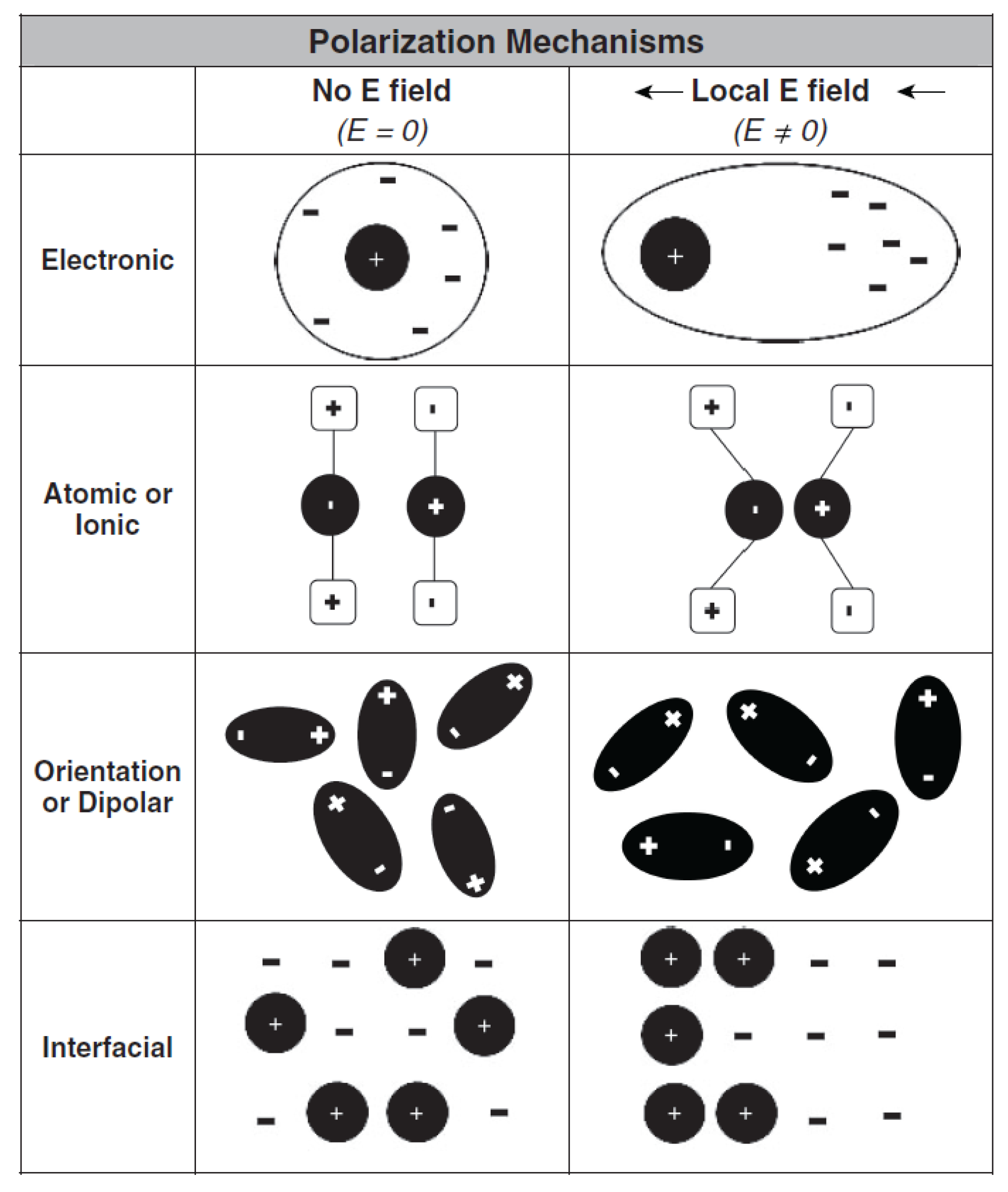
Dielectrics are generally classified into non-polar and polar dielectrics. Non-polar dielectrics are dielectrics that do not possess a permanent dipole moment; they become polarized in an electric field by relative displacement of electrons with respect to the nuclei [43,44]. This phenomenon is called electronic polarization (Figure 1), and the resonant process is typically observed at optical frequencies. Polar dielectrics are substances made up of molecules that possess inherent dipole moment. Accordingly, this class of dielectrics undergoes not only the electronic polarization, but also an atomic (or ionic) polarization, which is a change in the relative positions of atoms (or ions) in the manner depicted in Figure 1 [43,44]. Additionally, polar dielectrics may exhibit an orientation (or dipolar) polarization, where spatial reorientation of the permanent dipoles is induced by the electric field (Figure 1) [43,44].
In addition to the electronic, atomic and dipolar polarizations, there is another class of polarization termed interfacial (or space charge) polarization (Figure 1), which can be found in dielectrics having structural interfaces [43,44]. In the interfacial polarization, free charges accumulate at interfaces between two materials or between two regions of different electrical conductivities, and this separation of charges results in a local dipole moment [45]. Although the interfacial polarization could potentially exist in any materials having physical interfaces, this type of polarization usually appears only in the lower frequency regime because of the limited mobility of charges [45,46].
2.2. Permittivity
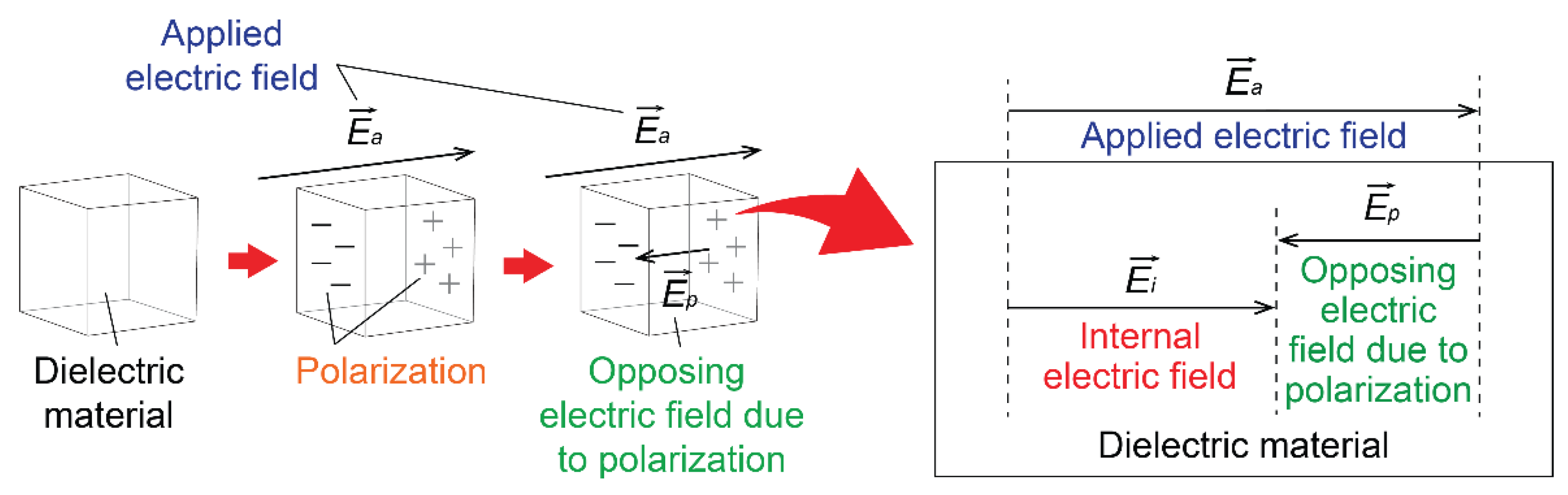
When an electric field is applied, a dielectric material responds by polarization; inside the dielectric medium, another electric field is generated in the opposite direction to the applied electric field as illustrated in Figure 2. As such, the electric field inside the dielectric material is reduced by this opposing electric field.
The strength of the internal electric field can be addressed by using the relative permittivity ()—a parameter by which the internal electric field is related to the applied electric field. The relationship is given by:
Accordingly, the strength of the opposing electric field can be written as:
It can be seen from the energy conservation point of view that the strength of this opposing electric field is the energy stored by the dielectric material. Upon removal from the external electric field, the polarized medium will undergo a depolarization process, where the relative positions of atoms and molecules return to the original, low energy state by releasing the stored energy.
During these storing and releasing processes, there are losses associated with the physical movements of atoms and molecules. As such, the relative permittivity of the physical dielectric materials is more formally written in the complex form () as [45]:
where and are the real and imaginary parts of the relative permittivity, respectively. The real part of the relative permittivity is also referred to as the dielectric constant and is a measure of the ability of a material to store the electric energy by polarization. The imaginary part of the relative permittivity is also known as the relative dielectric loss factor and quantifies the losses associated with the polarization. The tangent of the angle between the storage and loss components () is termed loss tangent and is expressed as [47]:
The loss tangent is a convenient index to assess the performance of dielectric materials-low-loss dielectrics with a large storage capacity exhibit a small loss tangent () while a large loss tangent () is due for lossy dielectrics that have a limited energy-storing capability [47].
2.3. Dispersion
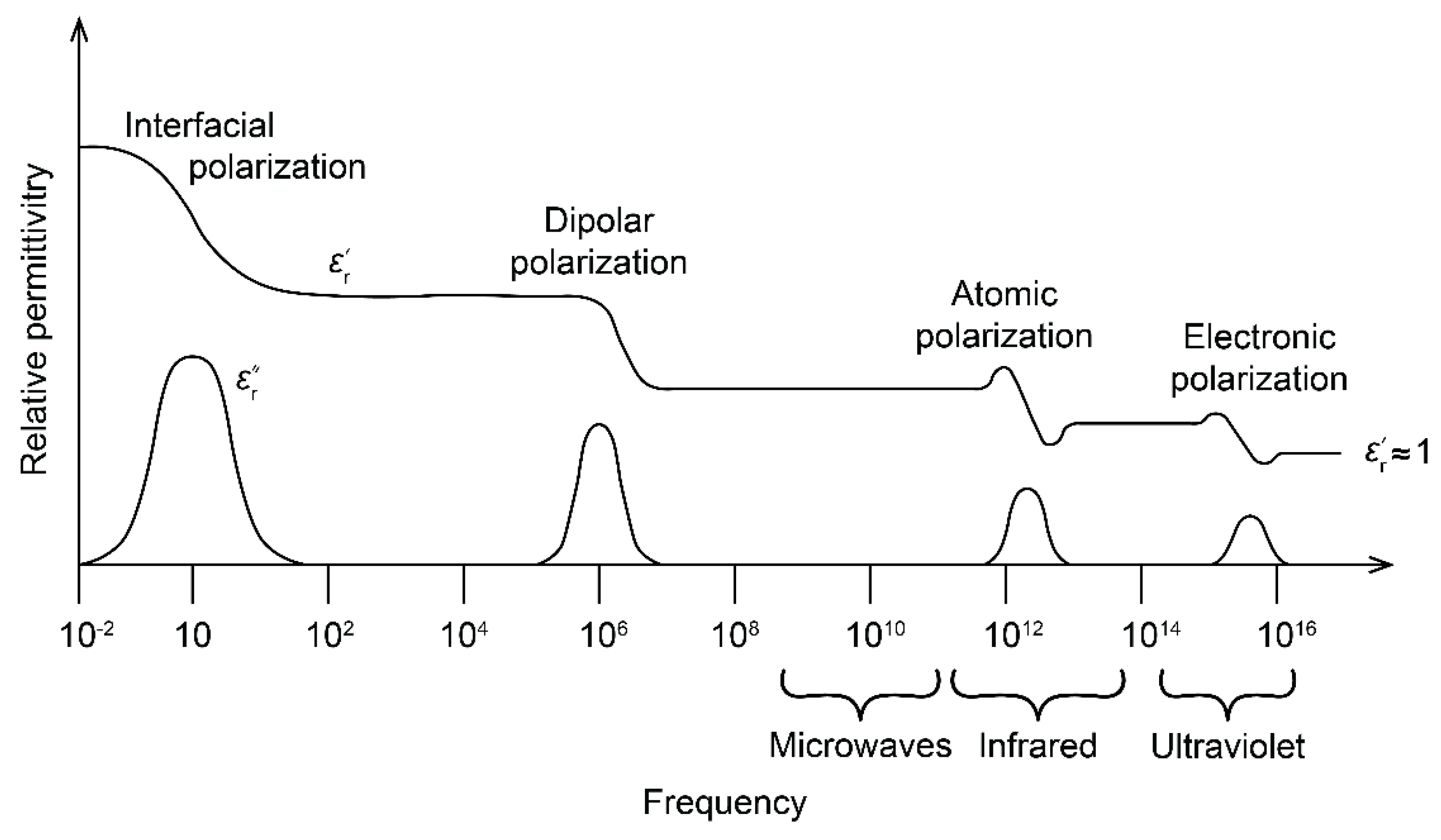
The physical mechanisms responsible for causing polarizations depend on the time variation of the electric field. In other words, the permittivity needs to be treated as a function of frequency of an alternating electric field. This frequency dependence of the permittivity is called dispersion and a representative curve is illustrated in Figure 3.
As the dispersion curve of shows, the relaxation process of the interfacial polarization is typically in the low frequency regime (10−2–102 Hz), whereas that of the dipolar polarization could be in the radio (105–107 Hz) frequency domain. These relaxations occur because of the limited mobility of space charges and permanent dipoles—as the frequency increases, these physical components will be too sluggish to respond [45]. For electronic and atomic polarizations, resonant processes are observed in the infrared and visible-ultraviolet regimes. The loss () peaks are associated with these relaxation and resonant processes.
With an aim to elucidate the dispersion characteristics, various models have been developed. For electronic and atomic polarizations, the Lorentz model [48] has been used extensively in literature. In this model, each atom is regarded to consist of a positive stationary charge surrounded by a mobile electron cloud, where the electron cloud experiences damping and tensional forces by an alternating electric field in an analogy to a mechanical spring [47]. The equation of motion is given by [47]:
where is the dipole charge; m is the mass of the electron cloud; is the displaced distance; is the time; is the friction (damping) coefficient; and is the tension (spring) coefficient. From this equation, the real and imaginary parts of the relative permittivity can be derived as a function of frequency, and the results are given by [47]:
where is the number of dipoles per unit volume and is the resonant angular frequency of the dielectric material.
Although the Lorentz model is widely used for its simplicity and explicitness, one critical limitation is that the model does not take the absorption into account [49]. Accordingly, the single Lorentzian oscillator is not suitable for examining absorbing materials such as amorphous solids and semiconductors, and more than one oscillator needs to be incorporated to analyze such dielectrics [49].
For dipolar polarizations, the Debye model [50] is often used to obtain the frequency dependence of the complex permittivity. In this model, molecules are assumed to be spherical in shape, and the real and imaginary parts of the relative permittivity are given, respectively, by [50]:
where and are the dielectric constants at a static frequency (i.e., the frequency just before the dipolar relaxation occurs) and at a much higher frequency (but not high enough to involve any resonant processes of electronic and atomic polarizations), respectively; and is the relaxation time. exhibits a peak when , and this peak is called the Debye loss peak. Many gaseous and some liquid materials with dipolar molecules are reported to follow the Debye relaxation model [45]. For most solids, however, this peak could become much broader because the loss cannot be expressed in terms of just a single well-defined relaxation time ; the relaxation in the solid is usually represented by a distribution of relaxation times [45]. In addition, Equations (8) and (9) assume that the dipoles do not influence each other either through their electric fields or through their interactions with the lattice; however, in solid dielectrics, dipoles can also couple, convoluting the relaxation process and limiting the accuracy of the Debye relaxation model [45].
Interfacial polarizations, on the other hand, are the results of the charges accumulated at the boundaries of different conductivities; accordingly, the shapes and geometries of the boundaries have substantial impact on the polarizability as well as the dispersion profile. In view of this, several dispersion theories were developed for different types of boundaries. One consequential premise is the Maxwell–Wagner theory, where spherical regions are considered to be sparsely dispersed in the medium of different conductivity [51]. According to this theory, the frequency-dependent complex relative permittivity is given by [51]:
where and are the real part of the relative permittivity of the inclusions and the environment, respectively; and are the electrical conductivities of the inclusions and the environment, respectively; is the volume fraction of the inclusion; is the angular frequency; and is the numerical factor (112.94 × 10¹¹).
For mixtures with ellipsoidal inclusions, the Maxwell–Wagner–Sillars model is often employed. This model is an extension of the Maxwell–Wagner model by Sillars [52] and incorporates an additional parameter that accounts for the eccentricity of the ellipsoids. Further details on the Maxwell–Wagner–Sillars model are available in [52].
While some of the most representative dispersion relationships have been discussed in this subsection, there are several notations. Firstly, for many dielectric materials, there could be more than just a single type of atoms and/or molecules. Secondly, microstructural configurations (e.g., crystalline and amorphous regions in polymers) make the atoms and molecules behave differently under the electric field [53,54]. As such, many dielectrics do not exhibit a simple, well-defined resonance or a relaxation process [45]. Analysis on the dispersion characteristic is usually of high complexity and requires technical proficiency because of these factors [41,46,55].
2.4. Anisotropy
The simple relationship between the applied electric field () and the internal electric field () given in Equation (1) is only valid when the polarization of a dielectric medium does not vary by the direction of the applied electric field. In both natural and artificial materials, however, there could exist microstructures that break the directional symmetry [8]. Such substances are called anisotropic materials; in an anisotropic medium, the internal electric field is oriented at an angle different from the applied electric field. On this account, Equation (1) becomes a second-rank tensor division for anisotropic materials as given by:
where is a second-rank, relative permittivity tensor. In the Cartesian coordinate, is expressed as a nine-entry matrix [47]:
where each entry (, , ··· ) represents an independent material parameter and may be a complex number. By using Equations (15) and (16), this can be rewritten as:
where , and are , and components of the applied electric field, respectively; and , and are , and components of the internal electric field, respectively. Equation (17) is the most generic form to express the permittivity of an anisotropic dielectric material.
In many practical cases, however, each entry is not necessarily unique. For example, a rectangular lattice that forms a basic structure in crystals may be expressed only in the three principal directions because of its biaxiality [8]. For uniaxial media, the permittivity component along the axis of crystal is different from the transversal permittivity, and thus it could have only one unique diagonal term in the permittivity matrix [8]. In addition to these symmetrical scenarios, for certain applications such as planar capacitors, transmission lines and antennas, the electric field is often limited to one principal direction [38,56,57]. If this is the case, then the permittivity may be considered only in such direction.
2.5. Inhomogenity and Homogenization
Inhomogeneity is another leading parameter in the science of dielectrics. When the permittivity is consistent regardless of the position within a material, the material is called homogeneous. On the other hand, if the permittivity varies as a function of position, this type of materials is called electrically non-homogeneous (heterogeneous) [8]. Often fiber-forming polymers are non-homogenous on the microstructural level since they could have both amorphous and crystalline regions that are characterized by different electrical polarizability [43]. In addition, mixtures of two or more components could be also non-homogeneous. For instance, a fabric may be considered as a non-homogeneous mixture of fiber and air [58]. Furthermore, materials having defects (e.g., voids) or impurities may also exhibit inhomogeneous behaviors on microscopic scale. Therefore, in many physical dielectrics, some degree of inhomogeneity potentially exists, and the permittivity may be more formally addressed as a function of position.
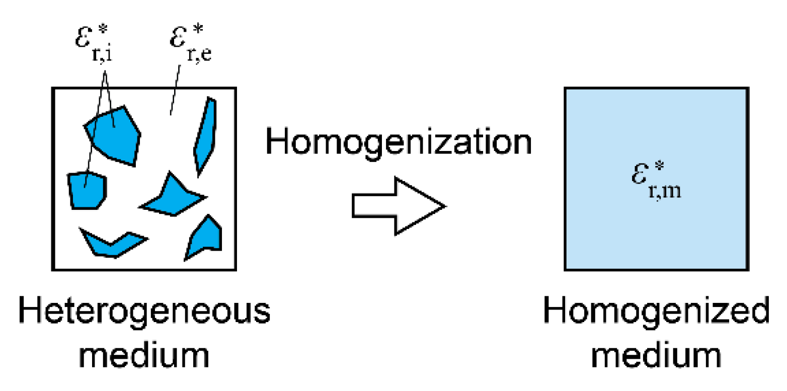
On one side, however, even such materials could be considered homogenous from the macroscopic point of view [8]. For example, when an observer is close enough to a woven fabric, the individual warp and weft yarns and their interlacing structure would be visible; however, when the fabric is placed far enough from the observer’s eyes, the detail structure of the fabric would no longer be recognizable, leaving an impression of just a uniform, homogenized sheet. Although the distance between the observer and the object was the parameter to describe the homogenization in this example, it is the wavelength (λ) of electromagnetic waves that critically distinguishes homogenized and non-homogenized substances in dielectric analysis [8]. In practice, the medium may be regarded homogenized when structural inhomogeneity is much smaller than ~0.1λ; the positional terms can then be dropped and a single, macroscopic permittivity value could be used [59,60,61]. This approach of describing microscopically heterogeneous dielectrics with a macroscopic, homogenized permittivity is called effective medium approximation [62,63] (Figure 4) and is the fundamental process in the dielectric mixture theory [64].
2.6. Dielectric Mixture Theory
The dielectric mixture theory is a statement of a relationship between the homogenized (macroscopic) dielectric properties of a heterogeneous medium and the local (microscopic) dielectric properties of its constituent materials (i.e., inclusions and environments) [64]. This relationship is expressed as a function of volume fractions of the components as an averaging factor. Since the geometry plays a pivotal role in the resulting dielectric properties of a heterogeneous medium, each dielectric mixture theory was developed for a specific geometry [8].
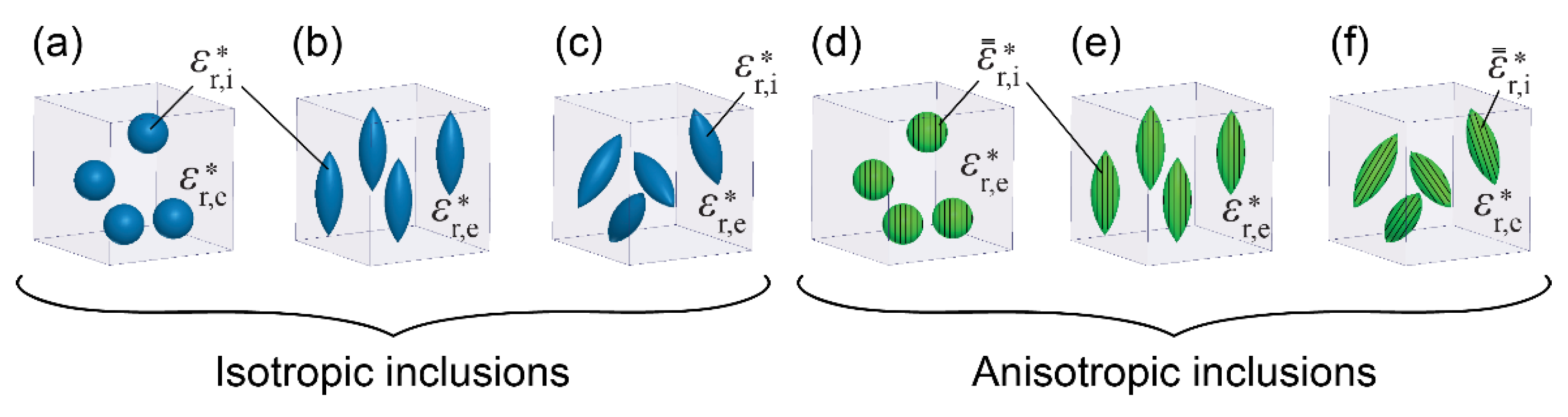
One of the most fundamental mixing theories is the Maxwell Garnett theory [65,66], which explicates the macroscopic complex relative permittivity () of a heterogeneous system of isotropic, spherical inclusions of complex relative permittivity randomly positioned in the environment of complex permittivity (Figure 5a). According to the theory, the macroscopic, complex relative permittivity is given by [65,66]:
where is the volume fraction of the spherical inclusions.
For many dielectrics, the spherical requirement for the inclusions needs to be relaxed—however, numerical effort is required for other shapes, and ellipsoids are among a few of the exceptions for which general analytical solutions can be obtained by extending the Maxwell Garnett theory [8]. For locally isotropic ellipsoids of permittivity randomly positioned in the environment (Figure 5b), its homogenized permittivity becomes a tensor if the ellipsoids are aligned. The x-component () of this permittivity tensor is given by [8]:
where is the volume fraction of the ellipsoidal inclusions; and is the depolarization factor in the direction of x-axis. Similarly, y- and z-components are given, respectively, by:
where and are depolarization factors in the corresponding axes and satisfy [8]:
Many natural and engineered materials possess this type of anisotropic structure, where the constituent materials themselves are isotropic in microscopic scale but the geometrical arrangement creates anisotropy [8].
For randomly oriented isotropic ellipsoids (Figure 5c), the macroscopic permittivity becomes a scalar as the directional terms are canceled. The expression is thus given by [8]:
So far, only isotropic inclusions are discussed. However, inclusions such as cotton fibers have anisotropic local permittivities due to the oriented polymer chains [67,68]. If this is the case, then the permittivity of inclusions needs to be treated as a second-rank tensor as discussed in this section. For inclusions of randomly positioned anisotropic spheres aligned in the environment (Figure 5d), the macroscopic permittivity tensor () is given by [8]:
where is the unit dyadic. Similarly, for inclusions of randomly positioned, but aligned anisotropic ellipsoids (Figure 5e), the macroscopic permittivity tensor is given by [8]:
where is the depolarization dyadic. Although not elaborated in detail in this paper, the macroscopic permittivity of inclusions of randomly positioned and randomly aligned anisotropic ellipsoids (Figure 5f) becomes a scalar, on a similar rationale to that of randomly positioned and randomly oriented isotropic ellipsoidal inclusions.
While the Maxwell Garnett theory and its extensions have been employed as powerful analytical tools for various dielectric mixtures, there are several limitations. For instance, the Maxwell Garnett theory assumes the inclusions to be small so that the interaction between the inclusions become negligible [69]. As such, the application of the Maxwell Garnett theory is practically limited to dilute systems [69].
The Bruggeman theory, on the other hand, is symmetric with respect to all medium components and can be applied to composites with arbitrary volume fractions without causing obvious geometrical contradictions [70]. For spherical inclusions of volume fraction fs, the macroscopic permittivity () is related to its constituent permittivities by [8]:
where and are the complex relative permittivities of the inclusions and environment, respectively. For randomly oriented ellipsoidal inclusions, the macroscopic permittivity () is given by [8]:
Another crucial theory in dielectric homogenization is the coherent potential theory. In this theory, the Green’s function enumerates the field of a given polarization density of the effective medium, leading to the relationship between the macroscopic and constituent permittivities. For the spherical inclusions, the coherent potential formula is given by [8]:
For randomly oriented ellipsoids of volume fraction , the coherent potential formula is given by [8]:
For dilute mixtures, all of the Maxwell Garnett, Bruggeman and coherent potential theories predict the same result. For spherical inclusions, those expressions are reduced to [8]:
In this subsection, the effects of the geometrical shapes, volume fractions and permittivities of various internal components on the homogenized dielectric properties were discussed based on the fundamental theories of dielectric mixtures. There is, however, an additional factor that could also hold an important role in the mixture analysis—interfacial polarization. Since mixtures involve at least two electrically non-identical components, the interfacial polarization could take place at the internal boundaries [6,41], but such a phenomenon is not considered in these theories. Yet, owing to its simplicity, explicitness and versatility the dielectric mixture theory has found a variety of uses, such as in analysis of chemical composition, structure and internal geometry and in designing composites with dielectric properties desirable for intended applications [41,42].
3. Dielectric Properties of Fabrics—The Air-Fiber System
In one view, textile materials are mixtures of fibers (or yarns) and air. Thus, by putting into the framework of the dielectric mixture theory, the dielectric properties of textile materials can be expressed as functions of the volume fraction and dielectric properties of the constituent fibers (or yarns). One of the early insights into this approach was presented by Bal and Kothari [39], who aimed to elucidate the dielectric properties of high-density polyethylene woven fabrics. In their work, measured dielectric constants of the woven fabrics were compared with those calculated by the dielectric mixing formulas. Although some of the mixing rules (e.g., the Maxwell Garnett formula) assume specific geometries and hence were not supposed to perfectly apply to woven fabrics, it was reported that any of the tested formulas predicted somewhat similar and acceptable results, most likely due to the fact that the volume fractions of the fabric samples were on the significantly lower side [39]. Later studies have demonstrated that the permittivity of textile materials could be dependent, not only on the volume fraction of fibers, but also on the fabric construction (e.g., woven versus knit) and fiber (yarn) orientation in a strict sense [5,6,7,40,41].
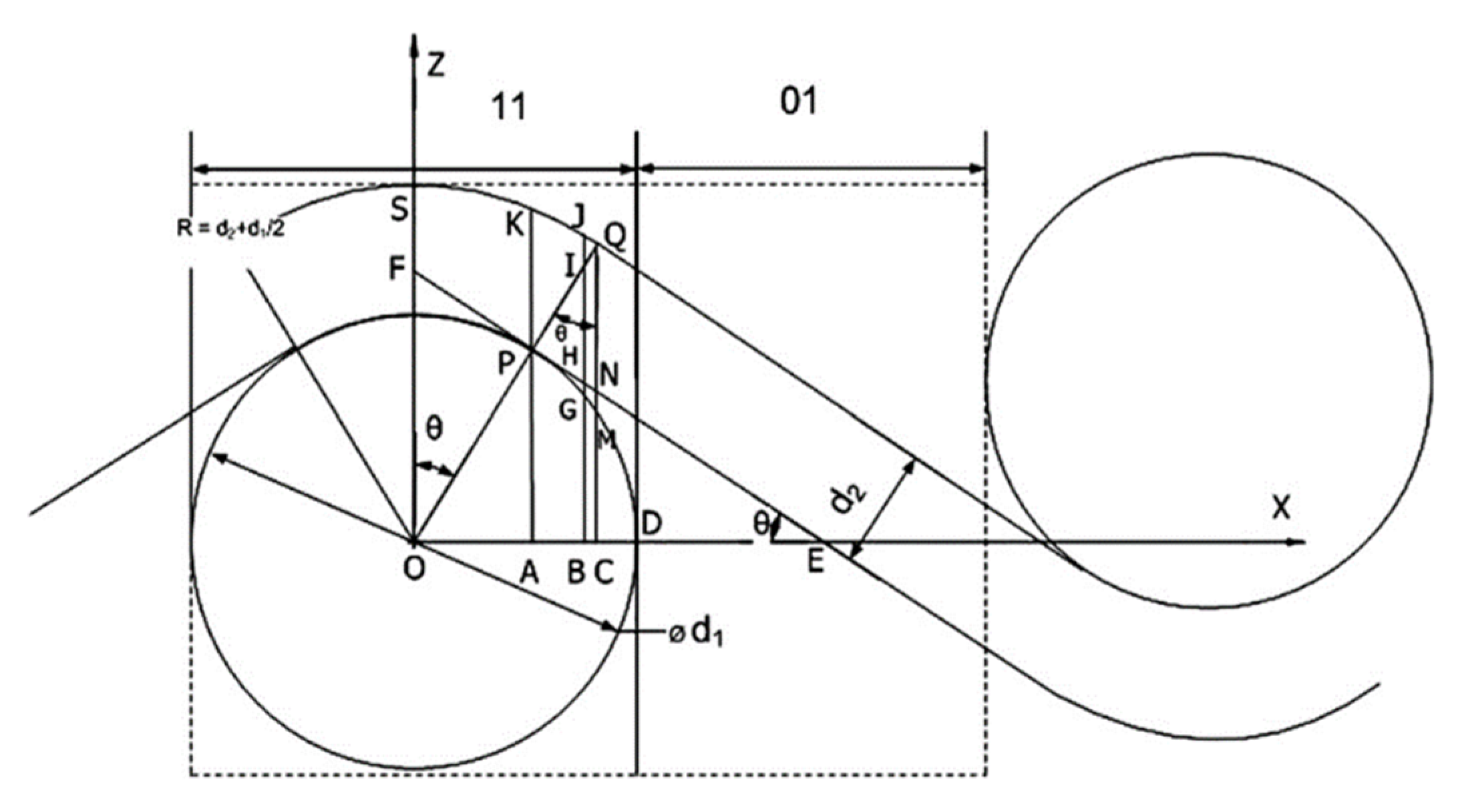
A model that represents a plain-woven fabric was proposed by Bal and Kothari [58] and is given in Figure 6. Based on the fundamental fabric geometry developed by Peirce [71], the repeating unit of the interlaced structure was considered to be the region encompassed by the rectangle in the schematic illustration. From this model, the capacitance () of a plain-woven fabric was formulated as [58]:
where and are the thread counts of warp and weft yarns, respectively; and are the spacings of the warp and weft yarns, respectively; and are the lengths of warp and weft yarns along the z-axis, respectively; and are the diameters of warp and weft yarns, respectively; and are the weaving angles of warp and weft yarns, respectively; is the fabric thickness; is the area of fabric; is the dielectric constant of the fiber; and is the absolute permittivity of free space. Because the capacitance is related to the dielectric constant by [57]:
the homogenized dielectric constant of a plain-woven fabric can be obtained by solving Equations (31) and (32). Based on comparisons to experimental data, the authors reported that this model predicted the dielectric constants of high-density polyethylene woven fabrics with reasonable accuracy [58].
Although not discussed in [57], this mathematical procedure of estimating the homogenized dielectric properties from fabric geometries and the permittivity of fibers (or yarns) may also be applied for staple or multifilament yarns if the macroscopic dielectric properties of such yarns are known. Moreover, it may be extended to cover broader types of fabric geometries such as various patterns of woven and knit fabrics by further elaborating the formulation.
4. Dielectric Properties of Fabrics—The Air-Fiber-Moisture System
The two-phase (air-fiber) models reviewed in Section 3 are applicable only for textile materials that are unaffected by moisture. Many natural (e.g., cotton, silk and wool) and artificial (e.g., polyamides) fibers, however, are hygroscopic and hence their dielectric properties can be radically altered by moisture [4,6,7,16,41,72,73]. The moisture absorbed by hygroscopic fibers is known to exist in two primary forms—free water and bound water [74,75]. Free water is water that has the thermodynamic state identical to the liquid (or bulk) water [76]. Bound water, on the other hand, takes the form chemically attached to a functional group of polymer chains, and thus the mobility of bound water is largely impeded [76]. Consequently, the electric polarizabilities of free and bound water are substantially different; the relaxation frequency of free water is observed in the gigahertz range [77,78], whereas bound water exhibits relaxation at much lower, megahertz frequencies because of the limited mobility [79,80]. Furthermore, absorbed water could drastically enhance the interfacial polarization by creating various types of boundaries with air and fiber [6,41].
Although the consideration of moisture is imperative in decent dielectric analysis of hygroscopic textile materials, the quantification and modeling of free and bound water is challenging. This is because the amounts, shapes and locations of free and bound water are intricately influenced by a number of factors including but not limited to temperature, relative humidity and microstructural profiles (e.g., crystallinity and porosity) [41,67,76,81,82,83]. Accordingly, most mixing models and theories available in literature are concerned with the moisture content without further distinction of its free and bound states.
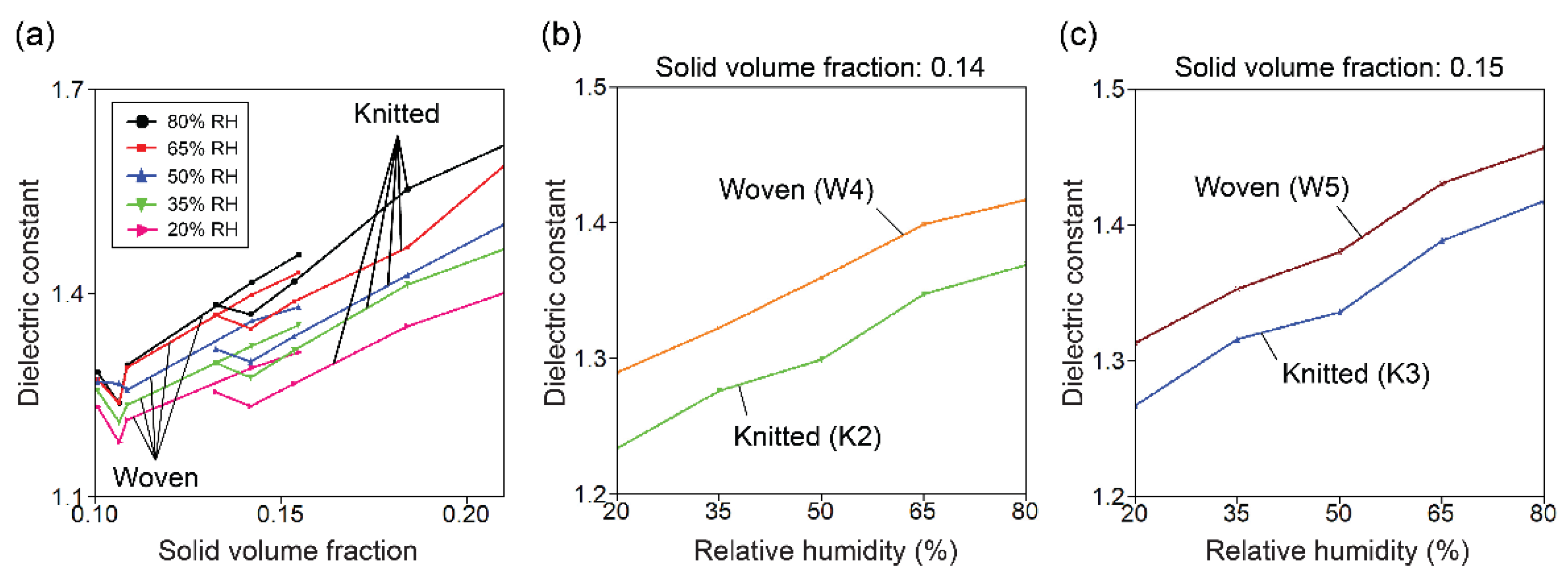
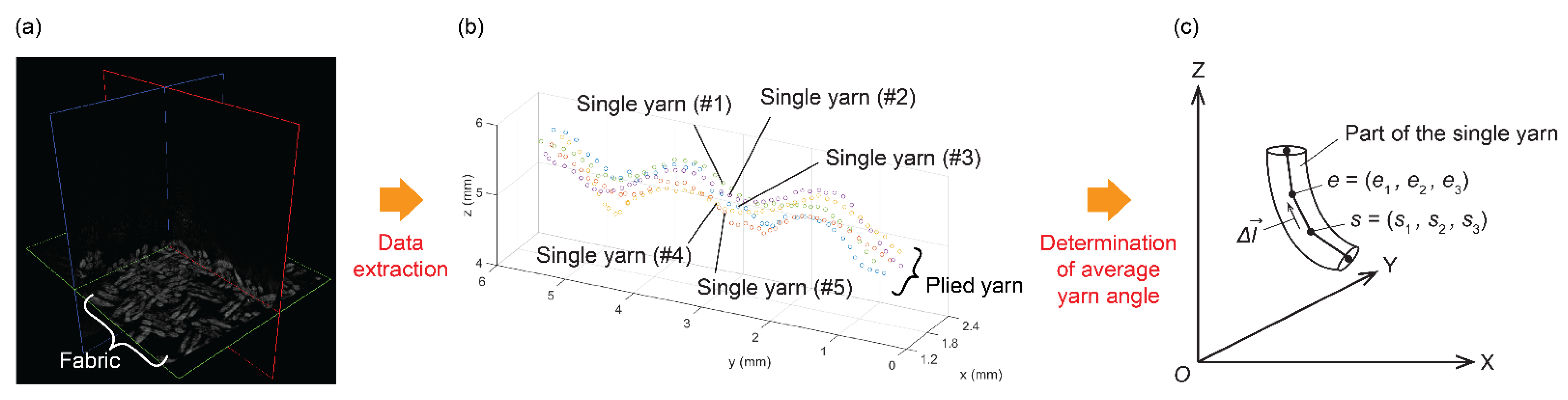
In a recent work, the relationship between the dielectric properties and the geometrical parameters were investigate for cotton fabrics at various relative humidity conditions [7]. Based on the out-of-plane dielectric characterization of woven and knitted fabric samples made of a five-ply cotton yarn, it was observed that the dielectric constant increases with the solid volume fraction (Figure 7a) [7]. It was also shown that the dielectric constant increases as the relative humidity increases (Figure 7a) [7], as reported in previous works [16,73]. Surprisingly, however, when the dielectric constants of the woven and knitted fabric samples of the same solid volume fractions were compared, the dielectric constants of woven samples were consistently higher than those of knitted samples (Figure 7b,c) [7]. This observation was substantiated by the evidence that the yarns (and hence fibers) in the woven samples were oriented more in the fabric thickness (out-of-plane) direction than in the case of knitted samples (Figure 8)—according to the extended Maxwell Garnett theory [8], the orientation of high aspect ratio materials affects the permittivity of the mixture and the permittivity in the fabric thickness direction will be higher if the fibers (yarns) are aligned more in this direction [7].
A theoretical model that predicts the dielectric properties of textile materials from the moisture content was proposed by Mukherjee in 2018 [84]. According to this model, the real () and imaginary () components of the relative permittivity are expressed as a function of moisture by:
where is the susceptibility; is the equilibrium order parameter; is the equilibrium polarization density; is the real part of the relative permittivity due to ionic and electronic polarizations; is the imaginary part of the relative permittivity due to ionic and electronic polarizations; is the moisture content; and are the temperature and supercooled temperature; and are the kinetic coefficients; and , , and are the Landau coefficients. The accuracy of this model was rigorously evaluated in a later work—the results obtained from this model were well comparable to the experimental data reported in the literature [85].
5. Measurement Methods
For the last couple of decades, methods for measuring the dielectric properties of textile materials have gained increasing interest. One critical facet has been its application in material characterization. Since the dielectric properties contain a wide range of information, such as the compositional, structural and geometrical properties, dielectric characterization could estimate these properties of textile materials [5,6,7,40,41,42], for instance for quality control of fabrics in a similar way to the capacitance-based fiber and yarn testing widely adopted in the textile industry [9,10,11,12,13,14]. Another unmissable application has been for development of textile-based wearable electronics. The performance and the form factor of electronic devices such as capacitors, transmission lines and antennas are well-documented to be impacted by the dielectric properties [38,47,57], and accordingly, the knowledge on the dielectric properties of textile materials is essential to design optimal textile-based electronics [7,15,41].
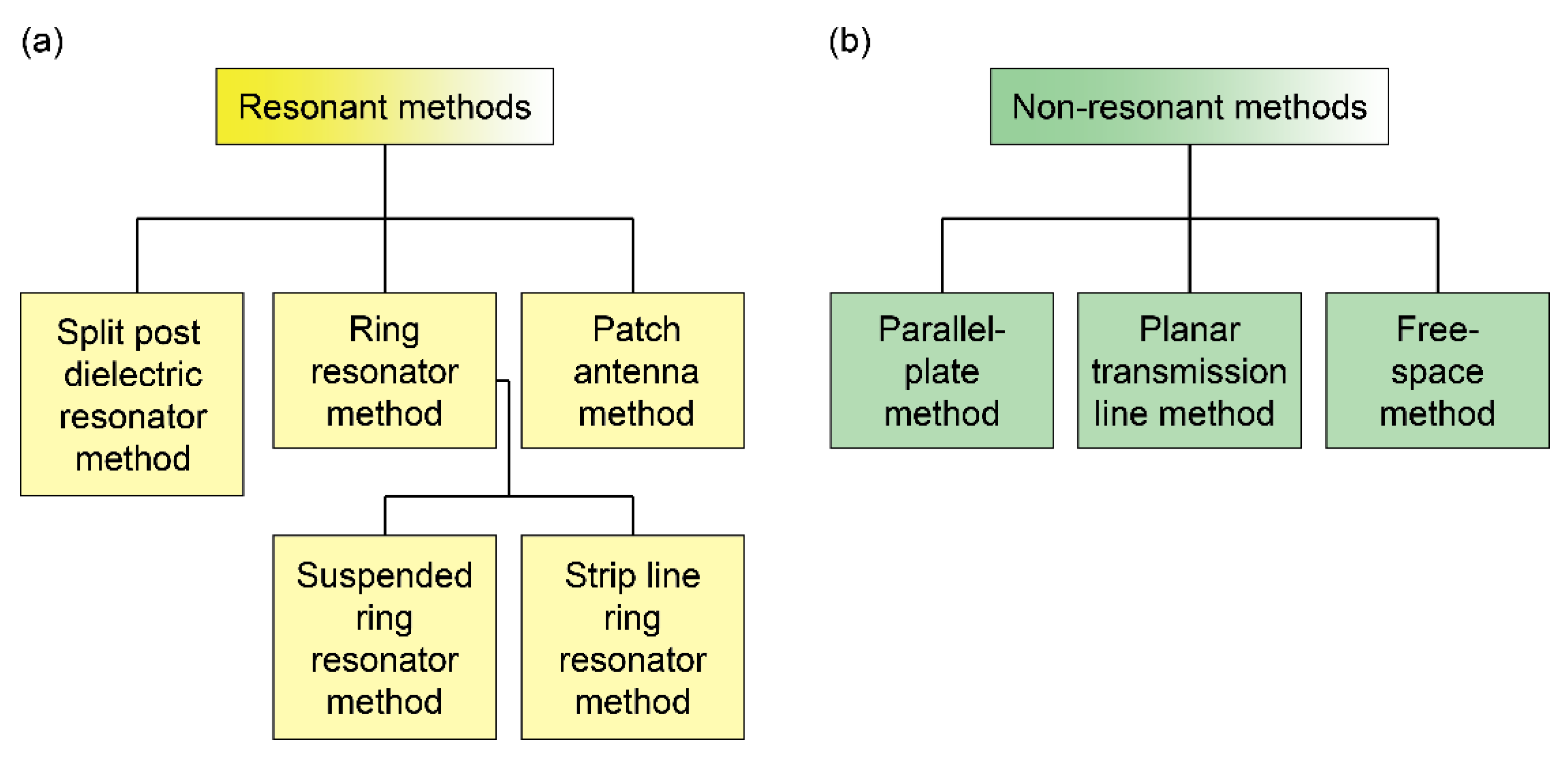
Dielectric characterization methods can be classified into the following two groups: resonant and non-resonant methods (Figure 9) [86,87]. In the resonant methods (Figure 9a), dielectric properties are determined through the measurement of resonant frequency and quality factor of resonant circuit embedded or covered with a dielectric material, whose dielectric properties are of interest [88]. Although resonant methods generally offer a higher level of accuracy and hence could be more suitable for low loss materials than the non-resonant methods, resonant methods can determine the dielectric properties only at a single or discrete set of frequencies [86,87]. Moreover, due to the physical size requirement of resonant structures, characterization is typically limited to certain microwave frequencies. Furthermore, since the resonant (and hence, the characterization) frequency is perturbed by the dielectric properties of the material under test, dielectric properties are often analyzed at a frequency that is slightly different from the target frequency [7,89].
Non-resonant methods (Figure 9b), on the other hand, could measure the dielectric properties in a broad range of frequency. The underlying principle in non-resonant methods is that electrical properties of a non-resonant circuit embedded or covered with a dielectric material are mathematically related to the dielectric properties. Although the measurement accuracy is generally limited in comparison with that of resonant methods, non-resonant methods offer information on the frequency-dependent dielectric properties. The following subsections review some of the most versatile dielectric characterization methods for textile materials from recent literature.
5.1. Resonant Methods
5.1.1. Split Post Dielectric Resonator Method
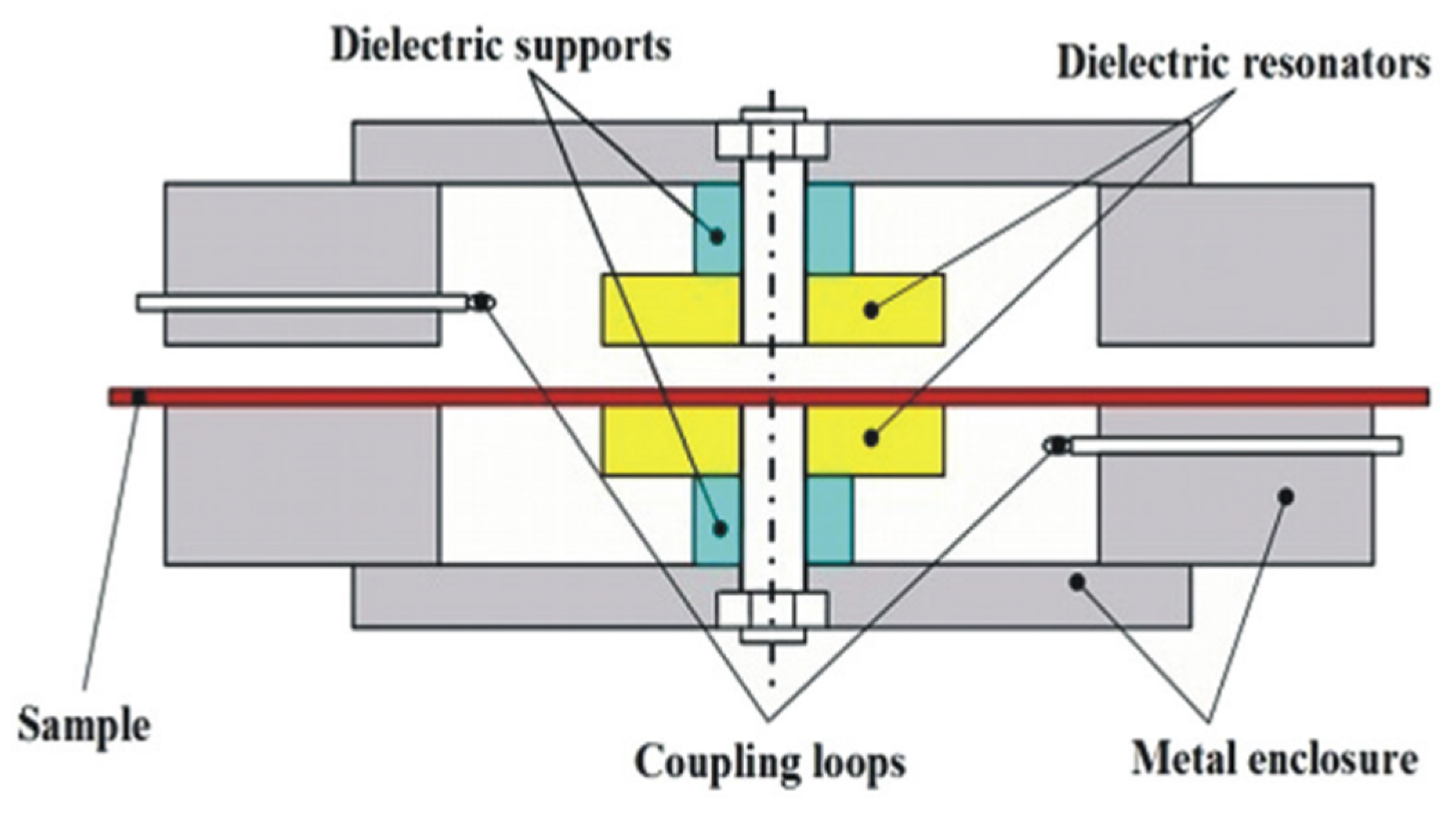
The split post dielectric resonator method employs a hollow enclosure (Figure 10) whose resonant frequencies and quality factors are pre-determined by its shape and dimensions, but which can be altered by placing a dielectric material inside it. The resonant frequencies and quality factors of the split post dielectric resonator are measured with and without a testing material (Figure 10) by using a vector network analyzer. The real part of the complex relative permittivity () can then be calculated from the shift in the resonant frequency by using the formula [90]:
where and are the resonant frequencies with and without sample, respectively; is the sample thickness; and is a function of and , and can be computed by an iterative method [90]. The loss tangent () can be obtained from the measured quality factors by using the expression [90]:
where is a quality factor of the sample-filled resonator; is the quality factor that accounts for the dielectric loss of the sample-filled resonator; is the quality factor that accounts for the conductor-related losses of the empty resonator; and and are functions of and and can be determined by an iterative method. Therefore, the imaginary part of the relative permittivity can be obtained by using Equations (4) and (40).
One considerable feature of the split post dielectric resonator method is that predefined, standard fixtures are commercially available on the market, and the complex relative permittivity of thin, planar materials, including fabrics, can be rapidly determined with excellent accuracy [92]. However, the characterization frequencies are typically limited to 1.1 to 20 GHz because of the physical size constraints of the fixture and testing material [92]. In addition, high permittivity samples need to be sufficiently thin to avoid undesirable resonances particularly at higher frequencies [93].
5.1.2. Ring Resonator Method
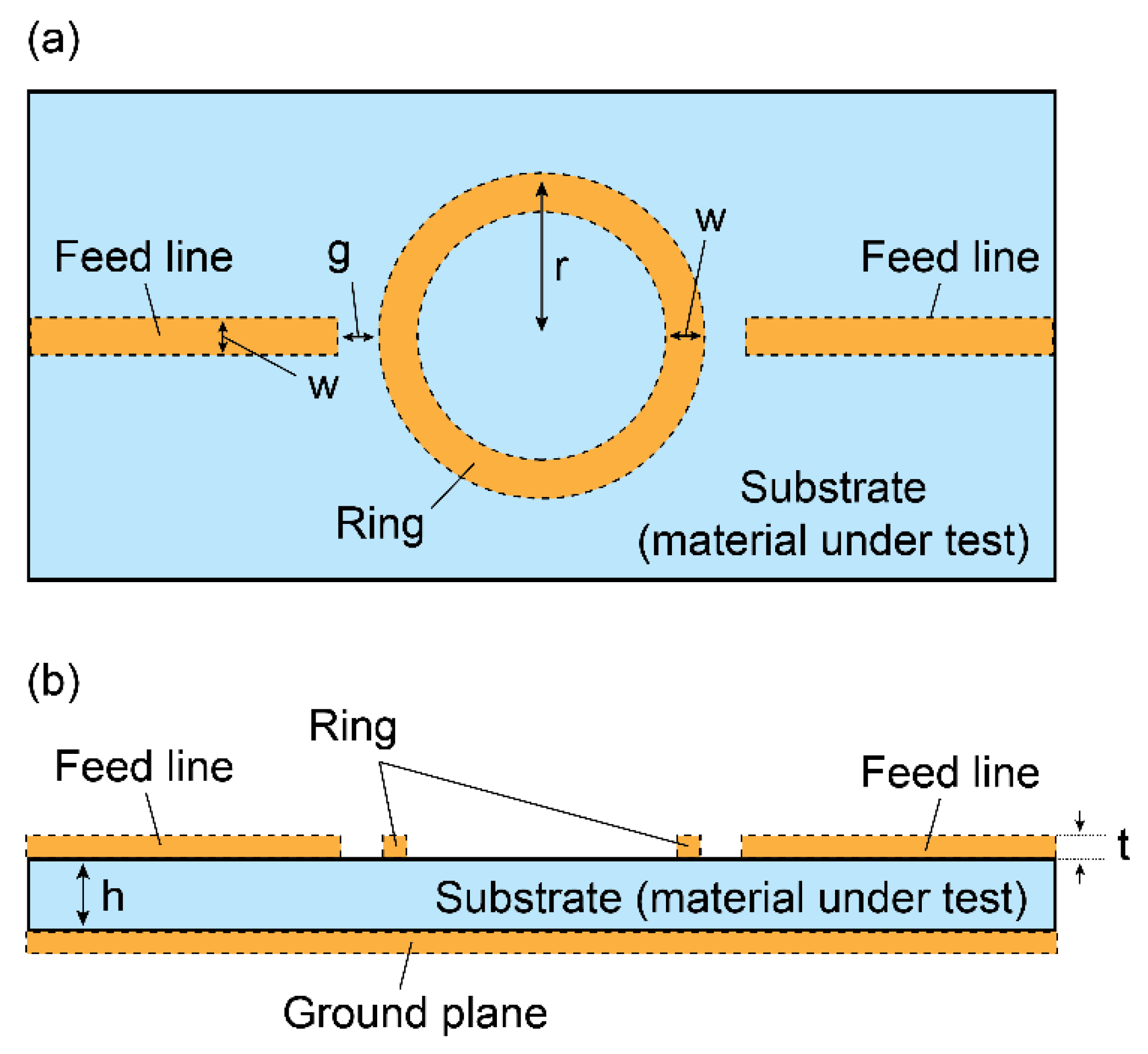
A ring resonator, as drawn in Figure 11, is a type of resonant structure whose resonant frequencies and quality factor in given dimensions are predominantly determined by the complex relative permittivity of the substrate [94]. Hence, in this method, the material under test is embedded as the substrate, and its complex relative permittivity is determined through the measurement of the resonant frequency and quality factor by using a vector network analyzer [94]. The real part of the relative permittivity () can be calculated from the resonant frequency of the ring resonator by using the expression [95]:
where is the resonant frequency of the ring resonator; is the radius of the ring; is the thickness of the material under test; and are the effective width and permittivity that account for the thickness of the strip (), respectively. The effective width and permittivity are given respectively by [95]:
The loss tangent () of the test sample can be obtained by [95]:
where is the wavelength of the free-space radiation from the ring at the resonant frequency; and is the attenuation due to the dielectric loss. can be obtained by subtracting the attenuation due to the conductor () and radiation () losses from the total attenuation () as [95]:
where is related to the quality factor of the ring resonator at the resonant frequency () by [95]:
can be determined by using the expression [95]:
where is the static conductivity of the ring; is the surface roughness; and is the skin depth. Since the radiation from the ring structure is typically negligibly small, the term can be dropped. Accordingly, the loss tangent of the testing material can be obtained by using Equations (44)–(47), and finally the imaginary part of the relative permittivity can be obtained by using Equation (4).
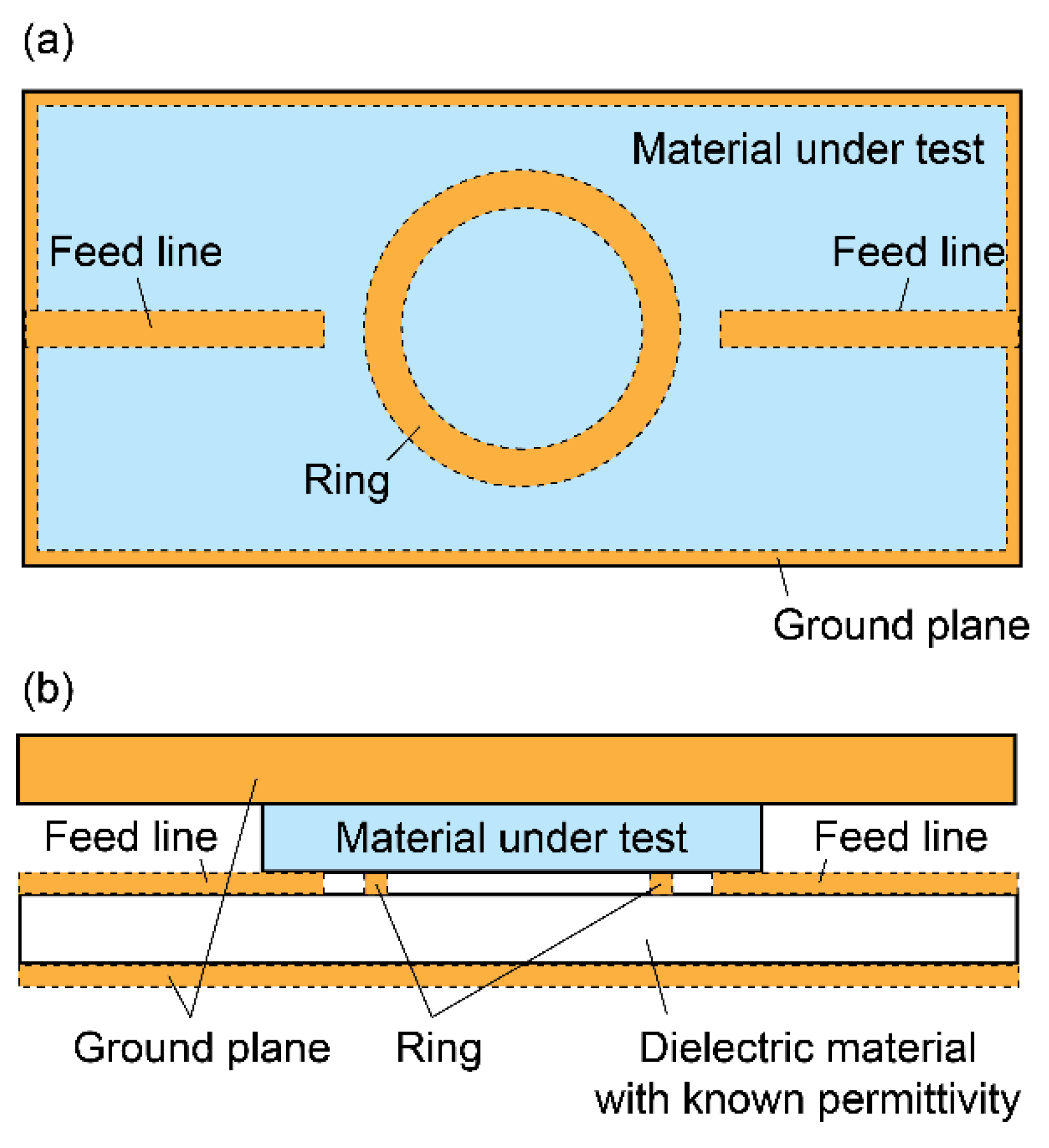
Although the ring resonator method could offer a good estimation of the complex relative permittivity in the microwave frequency domain, a preparatory phase is required to embed a testing material into the ring resonator geometry, but such process could be laborious and for certain samples even impracticable [94]. In order to ease the challenges in the sample preparation, multilayer methods such as the suspended ring resonator method and the strip line ring resonator method were proposed.
In the suspended ring resonator method, the ring resonator geometry is divided, for instance, into three sections, as follows: the lower layer, the sample, and the upper layer [94,96] (Figure 12). The lower layer consists of a ground plane and two feed lines mounted onto a dielectric medium of known complex permittivity, and the upper layer consist of the same dielectric material but this time with a ring. These lower and upper layers can be fabricated based on the conventional, printed circuit board technology. The sample is then placed in-between, and its complex relative permittivity can be determined through the measurements of the resonant frequency and quality factor in a similar manner to the original, ring resonator method. The specific formulas for the suspended ring resonator method are available in [94,96].
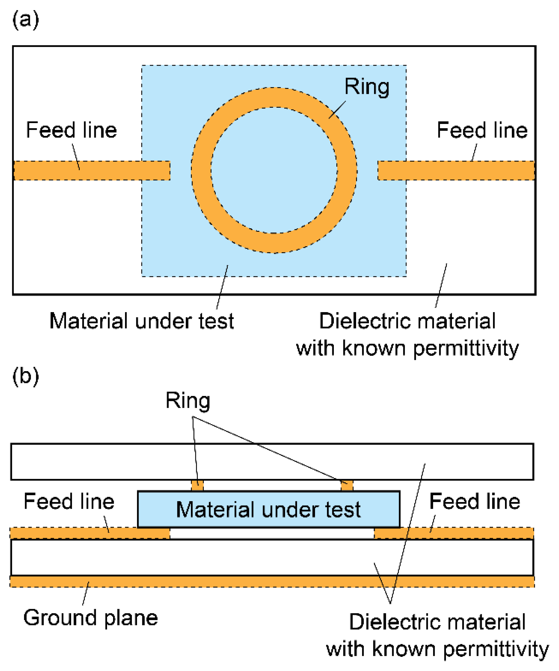
The strip line ring resonator method [97], on the other hand, employs a pre-established ring resonator, onto which the testing material is placed with a metal cover (Figure 13). The complex relative permittivity of the sample is then determined through the resonant frequency and quality factor measurements by using the formulas given in [97]. For both types of the multilayer ring resonator methods, ring resonator fixtures can be reused many times. Hence, these methods can be timesaving and cost-efficient alternatives to the original ring resonator method.
5.1.3. Patch Antenna Method
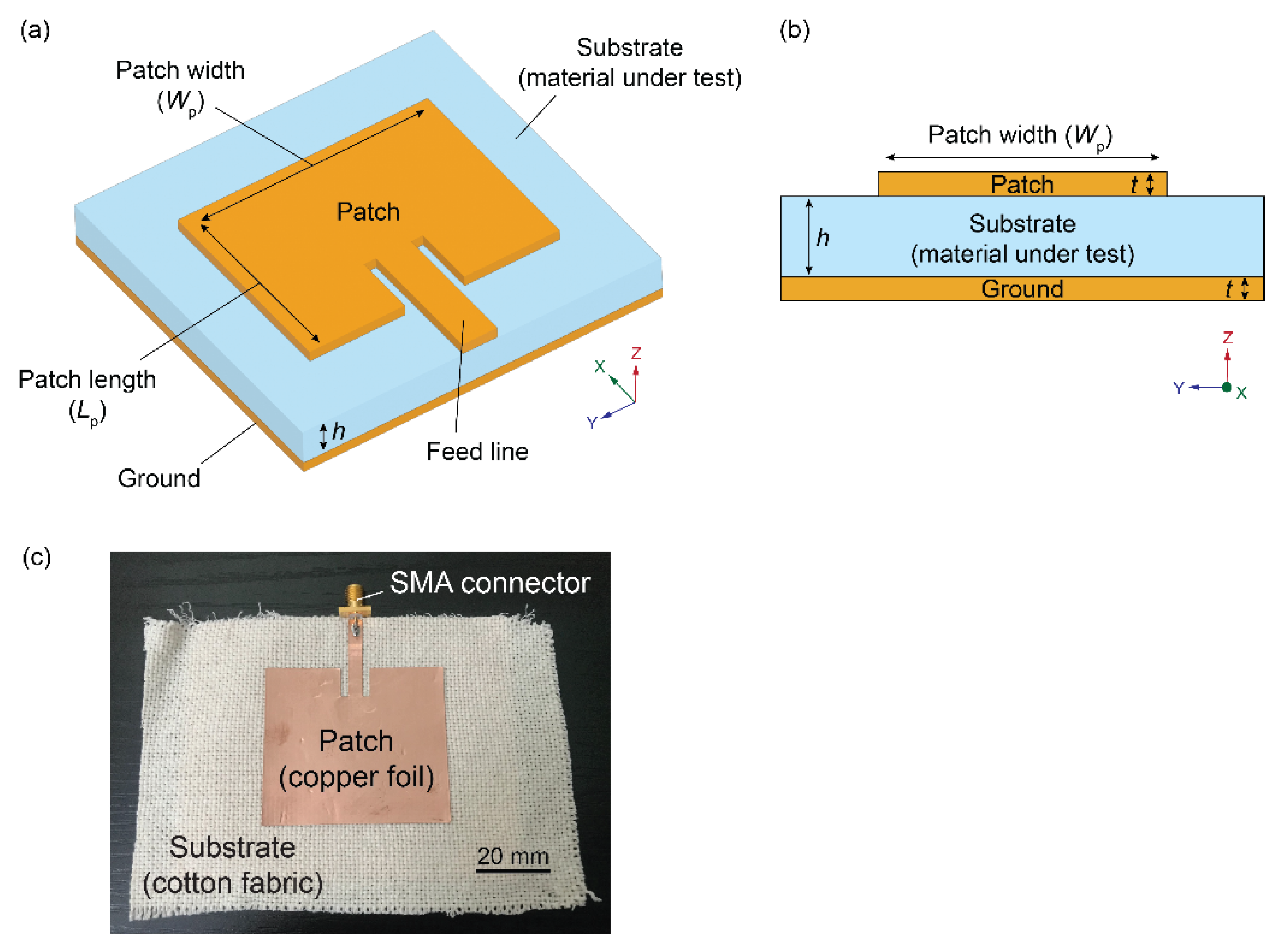
The patch antenna method is another resonant technique suitable for thin, planar samples including fabrics. The leading principle in this method is that a patch antenna, which consists of a conductive thin patch mounted on a grounded dielectric material, has a resonant frequency that is dependent on the dielectric constant of the substrate and antenna dimensions [38,47]; accordingly, the dielectric constant of the dielectric material can be estimated from the antenna dimensions and the measurement of the resonant frequency [5,7,41,89,98].
While various types of patch antennas could be designed for dielectric characterization, those in simple geometrical shapes such as rectangles are most commonly chosen for straightforward calculation. For a rectangular patch antenna depicted in Figure 14, the dielectric constant () of the test sample can be extracted from the analytical formula [41,89]:
where is the thickness of the test sample; is the width of the patch; and is the effective dielectric constant and can be calculated using the expression [41,89]:
where is the length of the patch and is the resonant frequency of the patch antenna.
It should be noted that while the patch antenna method could offer excellent accuracy in determining the real part of the relative permittivity [5,7,41,89,98], the imaginary part may not be acquired by this method. This is because typical patch antennas have non-negligible radiation and surface-wave losses, which are challenging to experimentally quantify. Therefore, the patch antenna method is primarily used for dielectric materials whose loss behavior is not of major concern [89] or in combination with another characterization method [41].
5.2. Non-Resonant Methods
5.2.1. Parallel-Plate Method
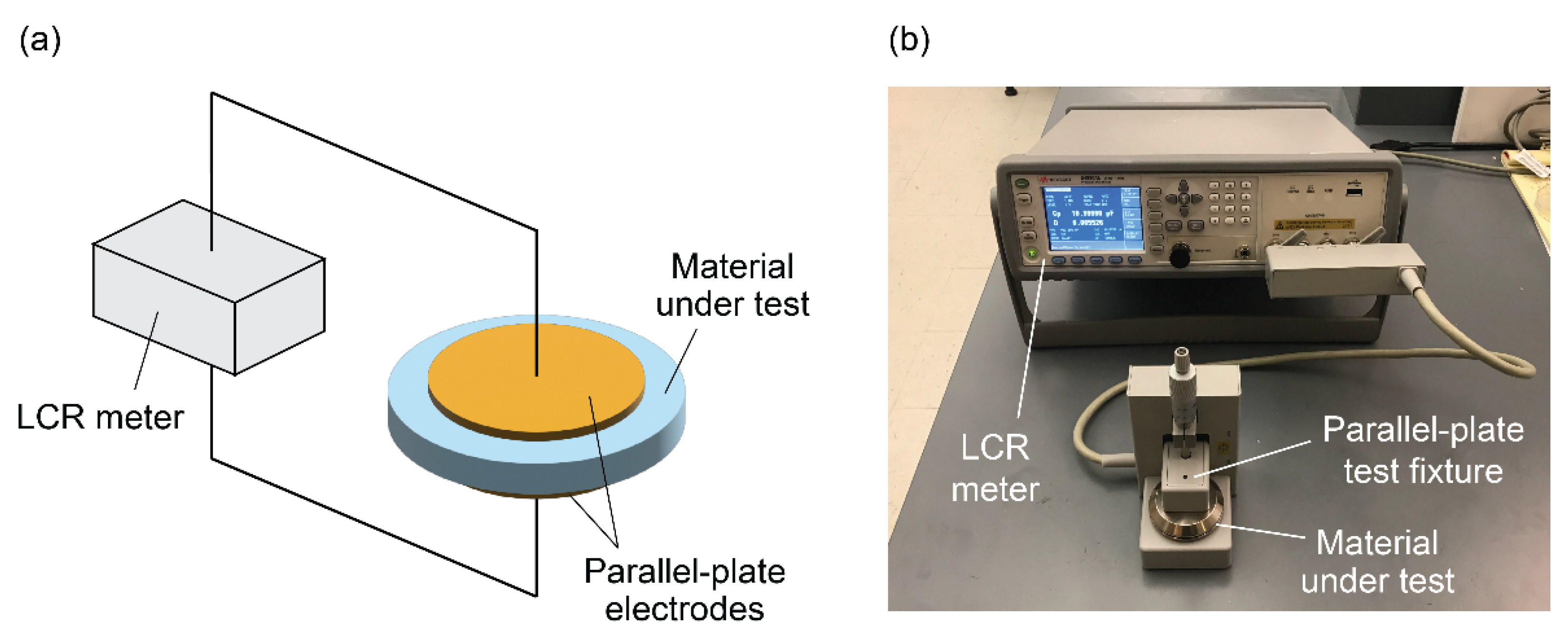
The parallel-plate method is one of the most common characterization methods in the low frequency regime typically below 1 GHz [86]. In this method, a sample is placed between a pair of electrodes and capacitance and dissipation factor () are measured by an LCR meter (Figure 15). The real part of the relative permittivity () is then calculated using the formula [57]:
where is the area of the electrode, and is the distance between the electrodes. For test samples whose static conductivities are negligibly small, the dissipation factor is equal to the loss tangent. Therefore, the imaginary part of the relative permittivity () can be calculated as [57]:
One critical advantage of the parallel-plate method is its simplicity in sample preparation and measurement setup [86]—samples in a wide range of thickness can be non-destructively measured with adjustable electrodes commercially available on the market. There is, however, one major notation in this method. It has been reported that charges accumulated at the sample-electrode interface during measurement could cause a large polarization (called electrode polarization) that mask the true response of the test sample [46]. This unwanted parasitic effect could be especially pronounced at lower frequencies for materials with high moisture contents including cotton fabrics [6,40,41], and can result in an extremely large, apparent complex permittivity [46]. Although several workarounds have been proposed to alleviate the effect of the electrode polarization [100,101,102,103], complete removal or compensation is almost unattainable.
5.2.2. Planar Transmission Line Method
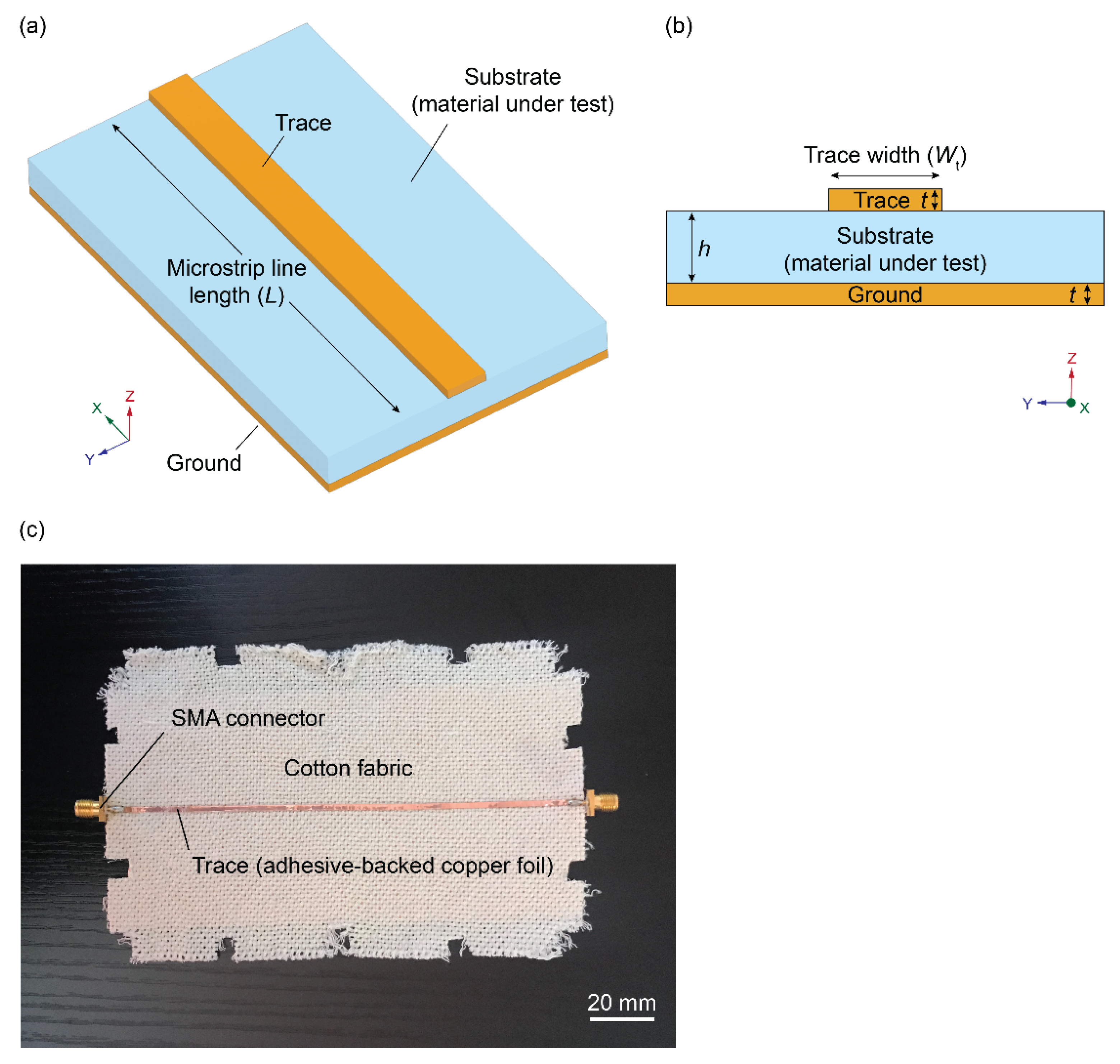
The planar transmission line method is a high-frequency technique that measures the complex permittivity of a thin test sample embedded in or placed in the vicinity of a planar transmission line. This method is based on the transmission line theory—the reflection and transmission characteristics of a planar transmission line is dependent on the dielectric properties of the embedded or the covered material [41,88,104]. Accordingly, the complex permittivity of the test material can be determined through the measurement of the reflection and transmission coefficients or the scattering parameters [41,88,104].
Planar transmission lines can be produced in various geometries; however, those in simple forms such as microstrip lines (Figure 16) are usually preferable for ease of fabrication and calculation. For the microstrip line geometry, the real part of the relative permittivity () is given by [41,56,105]:
where is the width of the trace; is the thickness of the sample; and is the effective dielectric constant given by [41,47]:
where is the phase constant. The phase constant can be calculated from the scattering parameters, which are measurable by a vector network analyzer with an appropriate calibration technique—the full details of the processes are described in [41].
The loss tangent can be calculated by the formula [41,105]:
where is the attenuation constant and can be calculated from the measured scattering parameters as described in [41]. The imaginary part of the relative permittivity can then be obtained from Equations (4) and (54).
Although there are several drawbacks, such as the necessity of calibration to remove the effect of feeding systems (e.g., connectors) and limited accuracy in characterization, one of the main features of the planar transmission line method is its simplicity in fabrication—for instance, planar transmission lines can be easily fabricated for a test sample by mounting thin conductive sheets such as a copper foil tape [41]. In addition, the frequency dependence of the complex permittivity can be acquired by this method since planar transmission lines support broadband microwave frequencies [106].
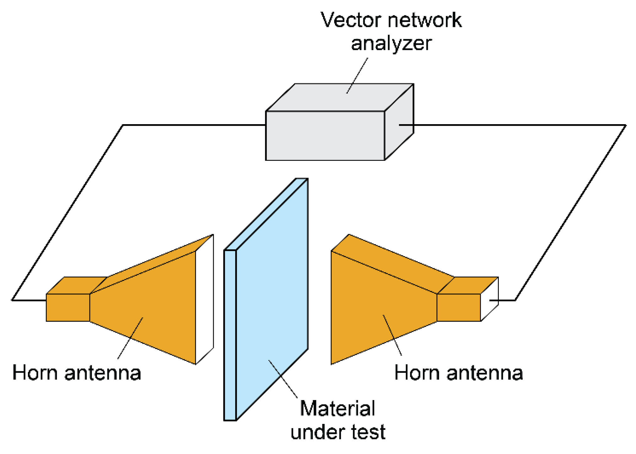
5.2.3. Free-Space Method
Another non-resonant method suitable for textile materials is the free space method, where a test specimen is placed between a pair of horn antennas connected to a vector network analyzer (Figure 17). Under this configuration, the complex relative permittivity () of the testing material is expressed as [107]:
where and are the cutoff and free-space wavelengths, respectively; is the sample thickness; is the complex relative permeability of the sample; and is the transmission coefficient. Since can be obtained from scattering parameter measurements with an appropriate calibration technique [107], the complex relative permittivity can be determined from Equation (55).
The major advantage of the free-space method is that the dielectric properties of sheet samples including textile materials can be non-destructively evaluated in the broad microwave frequencies simply by placing them between the horn antennas [107]. On the other hand, a calibration process is necessary to eliminate the effect of the feeding systems (e.g., connectors and antennas) in a similar rationale to the planar transmission method. In addition, a large sample surface is required to minimize the diffraction effects at the edges of the sample [109].
6. Conclusions
This paper reviewed various indispensable theories and principles related to the dielectric properties of textile materials. In order to provide a profound basis for unraveling the various intricate factors that affect the dielectric properties of textile materials, foundations on the dielectrics and polarization mechanisms were first recapitulated, followed by an overview on the concept of homogenization and some of the most prominent mixing rules. The key advantages, challenges and opportunities in the analytical approximations of the dielectric properties of textile materials were then discussed based on the findings and implications from the recent literature, and finally the variety of characterization methods were described for determination of the dielectric properties of textile materials.
Funding
This research received no external funding.
Conflicts of Interest
The author declares that there is no conflict of interest.
Appendix A

Table A1.
Dielectric properties of some pure fabrics reported in literature.
| Fabric Specification | Measurement Conditions | Dielectric Properties | Ref. | |||||||
|---|---|---|---|---|---|---|---|---|---|---|
| Composition | Construction | Solid Volume Fraction | Frequency (Hz) | Temperature (°C) | Relative Humidity (%) | Moisture Content (wt%) | Real Part | Imaginary Part | Loss Tangent | |
| Cotton | Plain weave | 0.134 * | 1 × 10⁶ | 21 | 40 | – | 5.59 | 0.352 ‡ | 0.063 | [73] |
| 60 | 6.12 | 0.514 ‡ | 0.084 | |||||||
| 80 | 7.08 | 0.722 ‡ | 0.102 | |||||||
| Cotton | Twill weave | 0.293 * | 2.45 × 10⁹ | – | – | – | 1.71 | 0.034 ‡ | 0.020 | [16] |
| Cotton | Plain weave | 0.10 | ~2.45 × 10⁹ | 21 ± 0.2 | 80 ± 2.5 | 8.42 | 1.28 | – | – | [7] |
| Plain weave | 0.11 | 1.24 | – | – | ||||||
| Plain weave | 0.11 | 1.29 | – | – | ||||||
| Plain weave | 0.14 | 1.42 | – | – | ||||||
| Plain weave | 0.15 | 1.46 | – | – | ||||||
| Cotton | Plain weave | 0.10 | ~2.45 × 10⁹ | 21 ± 2 | 65 ± 5 | 7.57 | 1.27 | – | – | [7] |
| Plain weave | 0.11 | 1.24 | – | – | ||||||
| Plain weave | 0.11 | 1.29 | – | – | ||||||
| Plain weave | 0.14 | 1.40 | – | – | ||||||
| Plain weave | 0.15 | 1.43 | – | – | ||||||
| Cotton | Plain weave | 0.10 | ~2.45 × 10⁹ | 21 ± 0.2 | 50 ± 2.5 | 6.43 | 1.27 | – | – | [7] |
| Plain weave | 0.11 | 1.27 | – | – | ||||||
| Plain weave | 0.11 | 1.26 | – | – | ||||||
| Plain weave | 0.14 | 1.36 | – | – | ||||||
| Plain weave | 0.15 | 1.38 | – | – | ||||||
| Cotton | Plain weave | 0.10 | ~2.45 × 10⁹ | 21 ± 0.2 | 35 ± 2.5 | 5.27 | 1.26 | – | – | [7] |
| Plain weave | 0.11 | 1.21 | – | – | ||||||
| Plain weave | 0.11 | 1.24 | – | – | ||||||
| Plain weave | 0.14 | 1.32 | – | – | ||||||
| Plain weave | 0.15 | 1.35 | – | – | ||||||
| Cotton | Plain weave | 0.10 | ~2.45 × 10⁹ | 21 ± 0.2 | 20 ± 2.5 | 3.77 | 1.23 | – | – | [7] |
| Plain weave | 0.11 | 1.18 | – | – | ||||||
| Plain weave | 0.11 | 1.21 | – | – | ||||||
| Plain weave | 0.14 | 1.29 | – | – | ||||||
| Plain weave | 0.15 | 1.31 | – | – | ||||||
| Cotton | Plain knit (single jersey) | 0.10 | ~2.45 × 10⁹ | 21 ± 0.2 | 80 ± 2.5 | 8.42 | 1.38 | – | – | [7] |
| Plain knit (single jersey) | 0.11 | 1.37 | – | – | ||||||
| Plain knit (single jersey) | 0.11 | 1.42 | – | – | ||||||
| Plain knit (single jersey) | 0.14 | 1.55 | – | – | ||||||
| Plain knit (single jersey) | 0.15 | 1.62 | – | – | ||||||
| Cotton | Plain knit (single jersey) | 0.10 | ~2.45 × 10⁹ | 21 ± 2 | 65 ± 5 | 7.57 | 1.37 | – | – | [7] |
| Plain knit (single jersey) | 0.11 | 1.35 | – | – | ||||||
| Plain knit (single jersey) | 0.11 | 1.39 | – | – | ||||||
| Plain knit (single jersey) | 0.14 | 1.47 | – | – | ||||||
| Plain knit (single jersey) | 0.15 | 1.59 | – | – | ||||||
| Cotton | Plain knit (single jersey) | 0.10 | ~2.45 × 10⁹ | 21 ± 0.2 | 50 ± 2.5 | 6.43 | 1.32 | – | – | [7] |
| Plain knit (single jersey) | 0.11 | 1.30 | – | – | ||||||
| Plain knit (single jersey) | 0.11 | 1.34 | – | – | ||||||
| Plain knit (single jersey) | 0.14 | 1.43 | – | – | ||||||
| Plain knit (single jersey) | 0.15 | 1.50 | – | – | ||||||
| Cotton | Plain knit (single jersey) | 0.10 | ~2.45 × 10⁹ | 21 ± 0.2 | 35 ± 2.5 | 5.27 | 1.30 | – | – | [7] |
| Plain knit (single jersey) | 0.11 | 1.28 | – | – | ||||||
| Plain knit (single jersey) | 0.11 | 1.32 | – | – | ||||||
| Plain knit (single jersey) | 0.14 | 1.41 | – | – | ||||||
| Plain knit (single jersey) | 0.15 | 1.47 | – | – | ||||||
| Cotton | Plain knit (single jersey) | 0.10 | ~2.45 × 10⁹ | 21 ± 0.2 | 20 ± 2.5 | 3.77 | 1.25 | – | – | [7] |
| Plain knit (single jersey) | 0.11 | 1.23 | – | – | ||||||
| Plain knit (single jersey) | 0.11 | 1.27 | – | – | ||||||
| Plain knit (single jersey) | 0.14 | 1.35 | – | – | ||||||
| Plain knit (single jersey) | 0.15 | 1.40 | – | – | ||||||
| Flax | Plain weave | 0.235 * | 1 × 10⁶ | 21 | 40 | – | 4.22 | 0.156 ‡ | 0.037 | [73] |
| 60 | 4.43 | 0.177 ‡ | 0.040 | |||||||
| 80 | 6.20 | 0.360 ‡ | 0.058 | |||||||
| Jute | Plain weave | 0.223 * | 1 × 10⁶ | 21 | 40 | – | 2.99 | 0.093 ‡ | 0.031 | [73] |
| 60 | 3.90 | 0.137 ‡ | 0.035 | |||||||
| 80 | 4.95 | 0.233 ‡ | 0.047 | |||||||
| Hemp | Plain weave | 0.249 * | 1 × 10⁶ | 21 | 40 | – | 4.08 | 0.114 ‡ | 0.028 | [73] |
| 60 | 4.50 | 0.162 ‡ | 0.036 | |||||||
| 80 | 4.77 | 0.248 ‡ | 0.052 | |||||||
| Wool | Plain weave | 0.303 * | 1 × 10⁶ | 21 | 40 | – | 4.11 | 0.115 ‡ | 0.028 | [73] |
| 60 | 4.65 | 0.214 ‡ | 0.046 | |||||||
| 80 | 5.70 | 0.296 ‡ | 0.052 | |||||||
| Polyester | 2 × 2 rib knit | – | 1.13 × 10³ | 20 ± 1 | 65 ± 2 | – | 4.06 | 1.67 | 0.46 | [110] |
| Polyester | Plain weave | 0.387 * | 1 × 10⁶ | 21 | 40 | – | 3.20 | 0.058 ‡ | 0.018 | [73] |
| 60 | 3.39 | 0.088 ‡ | 0.026 | |||||||
| 80 | 3.66 | 0.117 ‡ | 0.032 | |||||||
| Polyester | 3D spacer knit | 0.0706 * | 2.25× 10⁹ | – | – | – | 1.10 | 0.006 ‡ | 0.005 | [83] |
| Polyester | 3D spacer knit | 0.0821 * | 2.25× 10⁹ | – | – | – | 1.10 | 0.007 ‡ | 0.006 | |
| Polyester | 3D spacer knit | 0.0745 * | 2.25× 10⁹ | – | – | – | 1.12 | 0.019 ‡ | 0.017 | |
| Polyester | 3D spacer knit | 0.0982 * | 2.25× 10⁹ | – | – | – | 1.13 | 0.020 ‡ | 0.018 | |
| Polyester | 3D spacer knit | 0.0627 * | 2.25× 10⁹ | – | – | – | 1.11 | 0.004 ‡ | 0.004 | |
| Polyester | Plain weave | 0.43 † | 2.26 × 10⁹ | – | – | – | 1.55 | 0.013 ‡ | 0.009 | [111] |
| Polyester | Felt | – | 2.45 × 10⁹ | – | – | – | 1.2 | 0.028 ‡ | 0.023 | [24] |
| Polyester | Woven | – | – | – | – | 1.5 | 0.042 ‡ | 0.028 | ||
| Polyester | – | – | 2.45 × 10⁹ | – | – | – | 1.44 | – | – | [89] |
| Polyester | Fleece | 0.103 * | 2.45 × 10⁹ | – | – | 0.40 § | 1.15 | 0.000 ‡ | 0.000 | [16] |
| High density polyethylene | Plain weave | 0.1326 | 1 × 10³ | – | – | – | 1.12 | – | – | [39] |
| Plain weave | 0.1633 | 1 × 10³ | – | – | – | 1.14 | – | – | ||
| Plain weave | 0.1190 | 1 × 10³ | – | – | – | 1.10 | – | – | ||
| Plain weave | 0.2560 | 1 × 10³ | – | – | – | 1.23 | – | – | ||
* Calculated by the formula: φ = G/hρ, where φ is the solid volume fraction; G is the fabric weight; h is the fabric thickness; and ρ is the fiber density [6]. The commonly accepted values of 1.52 g/cm3 [112], 1.45 g/cm3 [113,114], 1.5 g/cm3 [115], 1.45 g/cm3 [116], 1.31 g/cm3 [117] and 1.39 g/cm3 [118,119] were used for the densities of cotton, flax, jute, hemp, wool and polyester fibers, respectively. † Calculated by the formula: φ = 1 − p/100, where p is the porosity (%) [120]. ‡ Calculated by Equation (4). § Calculated by M = 100R/(100 + R), where M and R are the moisture content (%) and the moisture regain (%), respectively [121].
References
- Bal, K.; Kothari, V.K. Measurement of Dielectric properties of textile materials and their applications. Indian J. Fibre Text. Res. 2009, 34, 191–199. [Google Scholar]
- Ivanovska, A.; Cerovic, D.; Maletic, S.; Jankovic Castvan, I.; Asanovic, K.; Kostic, M. Influence of the alkali treatment on the sorption and dielectric properties of woven jute fabric. Cellulose 2019, 26, 5133–5146. [Google Scholar] [CrossRef]
- Ivanovska, A.; Cerovic, D.; Tadic, N.; Jankovic Castvan, I.; Asanovic, K.; Kostic, M. Sorption and dielectric properties of jute woven fabrics: Effect of chemical composition. Ind. Crops Prod. 2019, 140, 111632. [Google Scholar] [CrossRef]
- Cerovic, D.D.; Petronijevic, I.; Dojcilovic, J.R. Influence of temperature and fiber structure on the dielectric properties of polypropylene fibrous structures. Polym. Adv. Technol. 2014, 25, 338–342. [Google Scholar] [CrossRef]
- Mukai, Y.; Suh, M. Structure-Microwave Dielectric Property Relationship in Cotton Fabrics. In Proceedings of the Techtextil North America, Raleigh, NC, USA, 26–28 February 2019. [Google Scholar]
- Mukai, Y.; Dickey, E.C.; Suh, M. Low Frequency Dielectric Properties Related to Structure of Cotton Fabrics. IEEE Trans. Dielectr. Electr. Insul. 2020, 27, 291–298. [Google Scholar] [CrossRef]
- Mukai, Y.; Suh, M. Relationships between Structure and Microwave Dielectric Properties in Cotton Fabrics. Mater. Res. Express 2020, 7, 015105. [Google Scholar] [CrossRef] [Green Version]
- Sihvola, A.H. Electromagnetic Mixing Formulas and Applications; IEE Electromagnetic Waves Series 47; Institution of Electrical Engineers: London, UK, 1999; ISBN 978-0-85296-772-0. [Google Scholar]
- Gandhi, K.L. Yarn Preparation for Weaving: Winding. In Woven Textiles; Elsevier: Amsterdam, The Netherlands, 2020; pp. 35–79. ISBN 978-0-08-102497-3. [Google Scholar]
- Carvalho, V.; Cardoso, P.; Belsley, M.; Vasconcelos, R.M.; Soares, F.O. Development of a Yarn Evenness Measurement and Hairiness Analysis System. In Proceedings of the IECON 2006-32nd Annual Conference on IEEE Industrial Electronics, Paris, France, 7–10 November 2006; pp. 3621–3626. [Google Scholar]
- Ghosh, A.; Mal, P. Testing of Fibres, Yarns and Fabrics and Their Recent Developments. In Fibres to Smart Textiles; Patnaik, A., Patnaik, S., Eds.; CRC Press: Boca Raton, FL, USA, 2019; pp. 221–256. ISBN 978-0-429-44651-1. [Google Scholar]
- Thilagavathi, G.; Karthik, T. Process Control and Yarn Quality in Spinning; Woodhead Publishing India in Textiles; CRC Press: Boca Raton, FL, USA, 2016; ISBN 978-93-80308-18-0. [Google Scholar]
- Ott, P.; Schmid, P. Verfahren und Vorrichtung zur Erkennung von Fremdstoffen in Einem Bewegten, Festen, Länglichen Prüfgut. European Patent EP2108949A1, 7 June 2006. [Google Scholar]
- ASTM D1425; Standard Test Method for Evenness of Textile Strands Using Capacitance Testing Equipment. ASTM International: West Conshohocken, PA, USA, 2014.
- Salvado, R.; Loss, C.; Gonçalves, R.; Pinho, P. Textile Materials for the Design of Wearable Antennas: A Survey. Sensors 2012, 12, 15841–15857. [Google Scholar] [CrossRef]
- Hertleer, C.; Laere, A.V.; Rogier, H.; Langenhove, L.V. Influence of Relative Humidity on Textile Antenna Performance. Text. Res. J. 2010, 80, 177–183. [Google Scholar] [CrossRef]
- Xu, F.; Zhu, H.; Ma, Y.; Qiu, Y. Electromagnetic performance of a three-dimensional woven fabric antenna conformal with cylindrical surfaces. Text. Res. J. 2017, 87, 147–154. [Google Scholar] [CrossRef]
- Mukai, Y.; Bharambe, V.T.; Adams, J.J.; Suh, M. Effect of bending and padding on the electromagnetic performance of a laser-cut fabric patch antenna. Text. Res. J. 2019, 89, 2789–2801. [Google Scholar] [CrossRef]
- Mukai, Y.; Suh, M. Development of a Conformal Woven Fabric Antenna for Wearable Breast Hyperthermia. Fash. Text. 2021, 8, 1–12. [Google Scholar] [CrossRef]
- Locher, I.; Klemm, M.; Kirstein, T.; Trster, G. Design and Characterization of Purely Textile Patch Antennas. IEEE Trans. Adv. Packag. 2006, 29, 777–788. [Google Scholar] [CrossRef] [Green Version]
- Mukai, Y.; Suh, M. Development of a Conformal Textile Antenna for Thermotherapy. In Proceedings of the Fiber Society’s Fall 2018 Technical Meeting and Conference, Davis, CA, USA, 29–31 October 2018. [Google Scholar]
- Mukai, Y.; Suh, M. Conformal Cotton Antenna for Wearable Thermotherapy. In Proceedings of the Fiber Society’s Spring 2019 Conference, Hong Kong, China, 21–23 May 2019. [Google Scholar]
- Jia, X.; Tennant, A.; Langley, R.J.; Hurley, W.; Dias, T. Moisture effects on a knitted waveguide. In Proceedings of the 2016 Loughborough Antennas & Propagation Conference (LAPC), Loughborough, UK, 14–15 November 2016; pp. 1–3. [Google Scholar]
- Adami, S.-E.; Proynov, P.; Hilton, G.S.; Yang, G.; Zhang, C.; Zhu, D.; Li, Y.; Beeby, S.P.; Craddock, I.J.; Stark, B.H. A Flexible 2.45-GHz Power Harvesting Wristband With Net System Output From −24.3 dBm of RF Power. IEEE Trans. Microw. Theory Tech. 2018, 66, 380–395. [Google Scholar] [CrossRef] [Green Version]
- Chi, Y.-J.; Lin, C.-H.; Chiu, C.-W. Design and modeling of a wearable textile rectenna array implemented on Cordura fabric for batteryless applications. J. Electromagn. Waves Appl. 2020, 34, 1782–1796. [Google Scholar] [CrossRef]
- Wagih, M.; Hilton, G.S.; Weddell, A.S.; Beeby, S. Broadband Millimeter-Wave Textile-Based Flexible Rectenna for Wearable Energy Harvesting. IEEE Trans. Microw. Theory Tech. 2020, 68, 4960–4972. [Google Scholar] [CrossRef]
- Zhang, R.Q.; Li, J.Q.; Li, D.J.; Xu, J.J. Study of the Structural Design and Capacitance Characteristics of Fabric Sensor. Available online: http://www.scientific.net/AMR.194-196.1489 (accessed on 6 June 2018).
- Seyedin, S.; Zhang, P.; Naebe, M.; Qin, S.; Chen, J.; Wang, X.; Razal, J.M. Textile strain sensors: A review of the fabrication technologies, performance evaluation and applications. Mater. Horiz. 2019, 6, 219–249. [Google Scholar] [CrossRef]
- Bansal, N.; Ehrmann, A.; Geilhaupt, M. Textile Capacitors as Pressure Sensors. In Proceedings of the Aachen-Dresden International Textile Conference, Dresden, Germany, 27–28 November 2014. [Google Scholar]
- Ma, L.; Wu, R.; Patil, A.; Zhu, S.; Meng, Z.; Meng, H.; Hou, C.; Zhang, Y.; Liu, Q.; Yu, R.; et al. Full-Textile Wireless Flexible Humidity Sensor for Human Physiological Monitoring. Adv. Funct. Mater. 2019, 29, 1904549. [Google Scholar] [CrossRef]
- Ng, C.; Reaz, M. Characterization of Textile-Insulated Capacitive Biosensors. Sensors 2017, 17, 574. [Google Scholar] [CrossRef] [PubMed] [Green Version]
- Liu, Y.; Yu, Y.; Zhao, X. The influence of the ratio of graphite to silver-coated copper powders on the electromagnetic and mechanical properties of single-layer coated composites. J. Text. Inst. 2021, 112, 1709–1716. [Google Scholar] [CrossRef]
- Liu, Y.; Yu, Y.; Zhao, X. The influence of wave-absorbing functional particles on the electromagnetic properties and the mechanical properties of coated fabrics. J. Text. Inst. 2021, 1–21. [Google Scholar] [CrossRef]
- Yamada, Y. Textile-Integrated Polymer Optical Fibers for Healthcare and Medical Applications. Biomed. Phys. Eng. Express 2020. [Google Scholar] [CrossRef]
- Yamada, Y.; Suh, M. Textile Materials for Mobile Health: Opportunities and challenges. In Proceedings of the WTiN Innovate Textile & Apparel Virtual Trade Show, Online, 15–30 October 2020. [Google Scholar]
- Wang, L.; Fu, X.; He, J.; Shi, X.; Chen, T.; Chen, P.; Wang, B.; Peng, H. Application Challenges in Fiber and Textile Electronics. Adv. Mater. 2020, 32, 1901971. [Google Scholar] [CrossRef] [PubMed]
- Hasan, M.M.; Hossain, M.M. Nanomaterials-patterned flexible electrodes for wearable health monitoring: A review. J. Mater. Sci. 2021, 56, 14900–14942. [Google Scholar] [CrossRef] [PubMed]
- Balanis, C.A. Antenna Theory: Analysis and Design, 4th ed.; Wiley: Hoboken, NJ, USA, 2016. [Google Scholar]
- Bal, K.; Kothari, V.K. Permittivity of woven fabrics: A comparison of dielectric formulas for air-fiber mixture. IEEE Trans. Dielectr. Electr. Insul. 2010, 17, 881–889. [Google Scholar] [CrossRef]
- Mukai, Y.; Suh, M. Effect of Fabric Construction, Thread Count and Solid Volume Fraction on the Dielectric Properties of Cotton Fabrics. In Proceedings of the Fiber Society’s Fall 2018 Technical Meeting and Conference, Davis, CA, USA, 29–31 October 2018. [Google Scholar]
- Mukai, Y. Dielectric Properties of Cotton Fabrics and Their Applications. Doctoral Dissertation, North Carolina State University, Raleigh, NC, USA, 2019. [Google Scholar]
- Giordano, S. Effective medium theory for dispersions of dielectric ellipsoids. J. Electrost. 2003, 58, 59–76. [Google Scholar] [CrossRef]
- Bunget, I.; Popescu, M. Physics of Solid Dielectrics; Materials Science Monographs 19; Elsevier: Amsterdam, The Netherlands, 1984; ISBN 978-0-444-99632-9. [Google Scholar]
- Gupta, M.; Wong, W.L. Microwaves and Metals; John Wiley & Sons: Singapore; Hoboken, NJ, USA, 2007; ISBN 978-0-470-82272-2. [Google Scholar]
- Kasap, S.O. Principles of Electronic Materials and Devices, 3rd ed.; McGraw-Hill: Boston, MA, USA, 2006; ISBN 978-0-07-295791-4. [Google Scholar]
- Kremer, F.; Schönhals, A. Broadband Dielectric Spectroscopy; Springer: Berlin/Heidelberg, Germany, 2003; ISBN 978-3-540-43407-8. [Google Scholar]
- Balanis, C.A. Advanced Engineering Electromagnetics, 2nd ed.; Wiley: Hoboken, NJ, USA, 2012; ISBN 978-0-470-58948-9. [Google Scholar]
- Oughstun, K.; Cartwright, N. On the Lorentz-Lorenz formula and the Lorentz model of dielectric dispersion. Opt. Express 2003, 11, 1541. [Google Scholar] [CrossRef]
- Patel, D.; Shah, D.; Hilfiker, J.; Linford, M. Characterization of Thin Films and Materials: A Tutorial on Spectroscopic Ellipsometry (SE) 5. Vac. Technol. Coat. 2019, 20, 34–37. [Google Scholar]
- Onimisi, M.Y.; Ikyumbur, J.T. Comparative Analysis of Dielectric Constant and Loss Factor of Pure Butan-1-ol and Ethanol. Am. J. Condens. Matter Phys. 2015, 5, 69–75. [Google Scholar]
- Hanai, T. Dielectric Theory on the Interfacial Polarization for Two-Phase Mixtures. Bull. Inst. Chem. Res. Kyoto Univ. 1962, 39, 341–367. [Google Scholar]
- Sillars, R.W. The properties of a dielectric containing semiconducting particles of various shapes. Inst. Electr. Eng-Proc. Wirel. Sect. Inst. 1937, 12, 139–155. [Google Scholar] [CrossRef]
- Arous, M.; Amor, I.B.; Kallel, A.; Fakhfakh, Z.; Perrier, G. Crystallinity and dielectric relaxations in semi-crystalline poly(ether ether ketone). J. Phys. Chem. Solids 2007, 68, 1405–1414. [Google Scholar] [CrossRef]
- Hikosaka, S.; Ishikawa, H.; Ohki, Y. Effects of crystallinity on dielectric properties of poly(L-lactide). Electron. Commun. Jpn. 2011, 94, 1–8. [Google Scholar] [CrossRef]
- Pelster, R. Dielectric relaxation spectroscopy in polymers: Broadband ac-spectroscopy and its compatibility with TSDC. In Proceedings of the 10th International Symposium on Electrets (ISE 10), Proceedings (Cat. No.99 CH36256), Athens, Greece, 22–24 September 1999; pp. 437–444. [Google Scholar]
- Bahl, I.J.; Trivedi, D.K. A designer’s guide to microstrip line. Microwaves 1977, 174–182. [Google Scholar]
- Natarajan, R. Power System Capacitors; Power Engineering 26; CRC Press: Boca Raton, FL, USA, 2005; ISBN 978-1-57444-710-1. [Google Scholar]
- Bal, K.; Kothari, V.K. Study of dielectric behaviour of woven fabric based on two phase models. J. Electrost. 2009, 67, 751–758. [Google Scholar] [CrossRef]
- Driscoll, T.; Basov, D.N.; Padilla, W.J.; Mock, J.J.; Smith, D.R. Electromagnetic characterization of planar metamaterials by oblique angle spectroscopic measurements. Phys. Rev. B 2007, 75, 115114. [Google Scholar] [CrossRef] [Green Version]
- Khoshman, J.M.; Kordesch, M.E. Vacuum Ultra-Violet Spectroscopic Ellipsometry Study of Sputtered BeZnO Thin Films. Optik 2011, 122, 2050–2054. [Google Scholar] [CrossRef]
- Jean-Mistral, C.; Sylvestre, A.; Basrour, S.; Chaillout, J.-J. Dielectric properties of polyacrylate thick films used in sensors and actuators. Smart Mater. Struct. 2010, 19, 075019. [Google Scholar] [CrossRef]
- Li, S.; Chen, R.; Anwar, S.; Lu, W.; Lai, Y.; Chen, H.; Hou, B.; Ren, F.; Gu, B. Applying effective medium theory in characterizing dielectric constant of solids. In Proceedings of the 2012 International Workshop on Metamaterials (Meta), Nanjing, China, 8–10 October 2012; pp. 1–3. [Google Scholar]
- Zhuromskyy, O. Applicability of Effective Medium Approximations to Modelling of Mesocrystal Optical Properties. Crystals 2016, 7, 1. [Google Scholar] [CrossRef] [Green Version]
- Tinga, W.R.; Voss, W.A.G.; Blossey, D.F. Generalized approach to multiphase dielectric mixture theory. J. Appl. Phys. 1973, 44, 3897–3902. [Google Scholar] [CrossRef]
- Garnett, J.C.M.; Larmor, J. XII. Colours in metal glasses and in metallic films. Philos. Trans. R. Soc. Lond. Ser. Contain. Pap. Math. Phys. Character 1904, 203, 385–420. [Google Scholar] [CrossRef]
- Sihvola, A. Homogenization principles and effect of mixing on dielectric behavior. Photonics Nanostruct.-Fundam. Appl. 2013, 11, 364–373. [Google Scholar] [CrossRef] [Green Version]
- Morton, W.E.; Hearle, J.W.S. Physical Properties of Textile Fibres; Woodhead Publishing: Sawston, UK, 2008; ISBN 978-1-84569-220-9. [Google Scholar]
- Balls, W.L. Dielectric Properties of Raw Cotton. Nature 1946, 158, 9–11. [Google Scholar] [CrossRef]
- Humlicek, J. Data Analysis for Nanomaterials: Effective Medium Approximation, Its Limits and Implementations. In Ellipsometry at the Nanoscale; Losurdo, M., Hingerl, K., Eds.; Springer: Berlin/Heidelberg, Germany, 2013; pp. 145–178. ISBN 978-3-642-33955-4. [Google Scholar]
- Markel, V.A. Introduction to the Maxwell Garnett approximation: Tutorial. J. Opt. Soc. Am. A 2016, 33, 1244. [Google Scholar] [CrossRef] [Green Version]
- Peirce, F.T. 5—The Geometry of Cloth Structure. J. Text. Inst. Trans. 1937, 28, T45–T96. [Google Scholar] [CrossRef]
- Bal, K.; Kothari, V.K. Dielectric behaviour of polyamide monofilament fibers containing moisture as measured in woven form. Fibers Polym. 2014, 15, 1745–1751. [Google Scholar] [CrossRef]
- Cerovic, D.D.; Dojcilovic, J.R.; Asanovic, K.A.; Mihajlidi, T.A. Dielectric investigation of some woven fabrics. J. Appl. Phys. 2009, 106, 084101. [Google Scholar] [CrossRef]
- Igarashi, T.; Hoshi, M.; Nakamura, K.; Kaharu, T.; Murata, K. Direct Observation of Bound Water on Cotton Surfaces by Atomic Force Microscopy and Atomic Force Microscopy–Infrared Spectroscopy. J. Phys. Chem. C 2020, 124, 4196–4201. [Google Scholar] [CrossRef] [Green Version]
- Sakabe, H.; Ito, H.; Miyamoto, T.; Inagaki, H. States of Water Sorbed on Wool as Studied by Differential Scanning Calorimetry. Text. Res. J. 1987, 57, 66–72. [Google Scholar] [CrossRef]
- Skaar, C. Wood-Water Relations; Springer Series in Wood Science; Springer: Berlin/Heidelberg, Germany, 1988; ISBN 978-3-642-73685-8. [Google Scholar]
- Buchner, R.; Barthel, J.; Stauber, J. The dielectric relaxation of water between 0 °C and 35 °C. Chem. Phys. Lett. 1999, 306, 57–63. [Google Scholar] [CrossRef]
- Hippel, A.R. von The dielectric relaxation spectra of water, ice, and aqueous solutions, and their interpretation. I. Critical survey of the status-quo for water. IEEE Trans. Electr. Insul. 1988, 23, 801–816. [Google Scholar] [CrossRef]
- Sugimoto, H.; Takazawa, R.; Norimoto, M. Dielectric relaxation due to heterogeneous structure in moist wood. J. Wood Sci. 2005, 51, 549–553. [Google Scholar] [CrossRef]
- Kuttich, B.; Grefe, A.-K.; Kröling, H.; Schabel, S.; Stühn, B. Molecular mobility in cellulose and paper. RSC Adv. 2016, 6, 32389–32399. [Google Scholar] [CrossRef] [Green Version]
- Cerovic, D.D.; Asanovic, K.A.; Maletic, S.B.; Dojcilovic, J.R. Comparative study of the electrical and structural properties of woven fabrics. Compos. Part B Eng. 2013, 49, 65–70. [Google Scholar] [CrossRef]
- Gezici-Koç, Ö.; Erich, S.J.F.; Huinink, H.P.; van der Ven, L.G.J.; Adan, O.C.G. Bound and free water distribution in wood during water uptake and drying as measured by 1D magnetic resonance imaging. Cellulose 2017, 24, 535–553. [Google Scholar] [CrossRef] [Green Version]
- Loss, C.; Gonçalves, R.; Pinho, P.; Salvado, R. Influence of some structural parameters on the dielectric behavior of materials for textile antennas. Text. Res. J. 2018. [Google Scholar] [CrossRef]
- Mukherjee, P.K. Dielectric properties in textile materials: A theoretical study. J. Text. Inst. 2018, 110, 1–4. [Google Scholar] [CrossRef]
- Mukherjee, P.K.; Das, S. Improved analysis of the dielectric properties of textile materials. J. Text. Inst. 2021, 112, 1890–1895. [Google Scholar] [CrossRef]
- Jilani, M.T.; Rehman, M.Z.; Khan, A.M.; Khan, M.T.; Ali, S.M. A Brief Review of Measuring Techniques for Characterization of Dielectric Materials. Int. J. Inf. Technol. Electr. Eng. 2012, 1, 5. [Google Scholar]
- Chen, L.F.; Ong, C.K.; Neo, C.P.; Varadan, V.V.; Varadan, V.K. Microwave Electronics: Measurement and Materials Characterization; Wiley: Chichester, UK, 2004. [Google Scholar]
- Baker-Jarvis, J. Dielectric and Conductor-Loss Characterization and Measurements on Electronic Packaging Materials; NIST Technical Note 1520; U.S. Department of Commerce, National Institute of Standards and Technology: Boulder, CO, USA, 2001.
- Sankaralingam, S.; Gupta, B. Determination of Dielectric Constant of Fabric Materials and Their Use as Substrates for Design and Development of Antennas for Wearable Applications. IEEE Trans. Instrum. Meas. 2010, 59, 3122–3130. [Google Scholar] [CrossRef]
- Mazierska, J.; Krupka, J.; Jacob, M.V.; Ledenyov, D. Complex permittivity measurements at variable temperatures of low loss dielectric substrates employing split post and single post dielectric resonators. In Proceedings of the 2004 IEEE MTT-S International Microwave Symposium Digest (IEEE Cat. No.04CH37535), Fort Worth, TX, USA, 6–11 June 2004; pp. 1825–1828. [Google Scholar]
- Kowerdziej, R.; Krupka, J.; Nowinowski-Kruszelnicki, E.; Olifierczuk, M.; Parka, J. Microwave complex permittivity of voltage-tunable nematic liquid crystals measured in high resistivity silicon transducers. Appl. Phys. Lett. 2013, 102, 102904. [Google Scholar] [CrossRef]
- Krupka, J.; Nguyen, D.; Mazierska, J. Microwave and RF methods of contactless mapping of the sheet resistance and the complex permittivity of conductive materials and semiconductors. Meas. Sci. Technol. 2011, 22, 085703. [Google Scholar] [CrossRef]
- Krupka, J. Microwave Measurements of Electromagnetic Properties of Materials. Materials 2021, 14, 5097. [Google Scholar] [CrossRef]
- Waldron, I. Ring Resonator Method for Dielectric Permittivity Measurement of Foams. Master’s Thesis, Worcester Polytechnic Institute, Worcester, MA, USA, 2006. [Google Scholar]
- Yang, L.; Rida, A.; Vyas, R.; Tentzeris, M.M. RFID Tag and RF Structures on a Paper Substrate Using Inkjet-Printing Technology. IEEE Trans. Microw. Theory Tech. 2007, 55, 2894–2901. [Google Scholar] [CrossRef] [Green Version]
- Waldron, I.; Makarov, S.N. Measurement of dielectric permittivity and loss tangent for bulk foam samples with suspended ring resonator method. In Proceedings of the 2006 IEEE Antennas and Propagation Society International Symposium, Albuquerque, NM, USA, 9–14 July 2006; pp. 3175–3178. [Google Scholar]
- Tu, H.; Zhang, Y.; Hong, H.; Hu, J.; Ding, X. A strip line ring resonator for dielectric properties measurement of thin fabric. J. Text. Inst. 2021, 112, 1772–1778. [Google Scholar] [CrossRef]
- Shimin, D. A New Method for Measuring Dielectric Constant Using the Resonant Frequency of a Patch Antenna. IEEE Trans. Microw. Theory Tech. 1986, 34, 923–931. [Google Scholar] [CrossRef]
- Rabih, A.A.S.; Begam, K.M.; Ibrahim, T.; Burhanudin, Z.A. Dielectric Properties of Properly Slaughtered and Non-properly Slaugheterd Chicken. J. Med. Res. Dev. 2014, 3, 15. [Google Scholar]
- Pizzitutti, F.; Bruni, F. Electrode and interfacial polarization in broadband dielectric spectroscopy measurements. Rev. Sci. Instrum. 2001, 72, 2502–2504. [Google Scholar] [CrossRef]
- Chassagne, C.; Dubois, E.; Jiménez, M.L.; van der Ploeg, J.P.M.; van Turnhout, J. Compensating for Electrode Polarization in Dielectric Spectroscopy Studies of Colloidal Suspensions: Theoretical Assessment of Existing Methods. Front. Chem. 2016, 4. [Google Scholar] [CrossRef]
- Ishai, P.B.; Talary, M.S.; Caduff, A.; Levy, E.; Feldman, Y. Electrode polarization in dielectric measurements: A review. Meas. Sci. Technol. 2013, 24, 102001. [Google Scholar] [CrossRef]
- Klein, R.J.; Zhang, S.; Dou, S.; Jones, B.H.; Colby, R.H.; Runt, J. Modeling electrode polarization in dielectric spectroscopy: Ion mobility and mobile ion concentration of single-ion polymer electrolytes. J. Chem. Phys. 2006, 124, 144903. [Google Scholar] [CrossRef] [PubMed]
- Gupta, K.C.; Ramadoss, R.; Zhang, H. RF and microwave network characterization-a concept-map-based tutorial. IEEE Trans. Microw. Theory Tech. 2003, 51, 1326–1329. [Google Scholar] [CrossRef]
- Ravelo, B.; Thakur, A.; Saini, A.; Thakur, P. Microstrip Dielectric Substrate Material Characterization with Temperature Effect. Appl. Comput. Electromagn. Soc. 2015, 30, 1322–1328. [Google Scholar]
- Maloratsky, L.G. Reviewing The Basics Of Microstrip Lines A. Microw. RF 2000, 39, 79–88. [Google Scholar]
- Rocha, L.S.; Junqueira, C.C.; Gambin, E.; Nata Vicente, A.; Culhaoglu, A.E.; Kemptner, E. A free space measurement approach for dielectric material characterization. In Proceedings of the 2013 SBMO/IEEE MTT-S International Microwave & Optoelectronics Conference (IMOC), Rio de Janeiro, Brazil, 4–7 August 2013; pp. 1–5. [Google Scholar]
- Fwen, W.; Ping, S.; Abd Malek, M.F.; Hasss, N. Alternatives for PCB Laminates: Dielectric Properties’ Measurements at Microwave Frequencies. In Dielectric Material; Silaghi, M.A., Ed.; InTech: Rijeka, Croatia, 2012; ISBN 978-953-51-0764-4. [Google Scholar]
- Pometcu, L.; Sharaiha, A.; Benzerga, R.; Tamas, R.D.; Pouliguen, P. Method for material characterization in a non-anechoic environment. Appl. Phys. Lett. 2016, 108, 161604. [Google Scholar] [CrossRef]
- Liu, Y.; Zhao, X. Influence of the Yarn Fineness and Stitch Length of Polyester Knitted Fabric on the Dielectric Constant. Fibres Text. East. Eur. 2019, 27, 63–66. [Google Scholar] [CrossRef]
- Mukai, Y.; Bharambe, V.T.; Adams, J.J.; Suh, M. Effect of Bending and Padding on the Electromagnetic Performance of a Laser-Cut Woven Fabric Patch Antenna. In Proceedings of the Textiles Research Open House, Raleigh, NC, USA, 16 April 2018. [Google Scholar]
- Shao, X.; Qiu, Y.; Wang, Y. Theoretical modeling of the tensile behavior of low-twist staple yarns: Part II–theoretical and experimental results. J. Text. Inst. 2005, 96, 69–76. [Google Scholar] [CrossRef]
- Van de Velde, K.; Kiekens, P. Development of a Flax/Polypropylene Composite with Optimal Mechanical Characteristics by Fiber and Matrix Modification. J. Thermoplast. Compos. Mater. 2002, 15, 281–300. [Google Scholar] [CrossRef]
- Van de Velde, K.; Kiekens, P. Influence of Fibre and Matrix Modifications on Mechanical and Physical Properties of Flax Fibre Reinforced Poly(propylene). Macromol. Mater. Eng. 2001, 286, 237–242. [Google Scholar] [CrossRef]
- Dalbehera, S.; Acharya, S.K. Study on mechanical properties of natural fiber reinforced woven jute-glass hybrid epoxy composites. Adv. Polym. Sci. Technol. 2014, 4, 1–6. [Google Scholar]
- Wang, L.; Kumar, R.; Zhang, L. Investigation into hemp fiber- and whisker-reinforced soy protein composites. Front. Chem. China 2009, 4, 313–320. [Google Scholar] [CrossRef]
- Li, Y.V. Proteins and Protein-Based Fibers. In ACS Symposium Series; Yang, Y., Xu, H., Yu, X., Eds.; American Chemical Society: Washington, DC, USA, 2014; Volume 1175, pp. 21–36. ISBN 978-0-8412-2990-7. [Google Scholar]
- Xiang, P.; Kuznetsov, A.V.; Seyam, A.-F.M. Simulation of Fiber Entanglement by Modeling Vorticity in Water Flow Field. Text. Res. J. 2007, 77, 312–329. [Google Scholar] [CrossRef]
- Shaikh, T.N.; Bhattacharya, S.S. Deriving an empirical formula to determine the optimum level of false-twist in mechanically-crimped textured polyester yarn. Text. Res. J. 2011, 81, 1995–2005. [Google Scholar] [CrossRef]
- Mao, N.; Russell, S.J. Fibre to Fabric: Nonwoven Fabrics-ScienceDirect. In Textiles and Fashion; Woodhead Publishing Limited: Sawston, UK, 2015; pp. 307–335. ISBN 978-0-85709-561-9. [Google Scholar]
- ASTM D2495-17; Standard Test Method for Moisture in Cotton by Oven-Drying. ASTM International: West Conshohocken, PA, USA, 2012.
Figure 1.
Polarization mechanisms. Reprinted with permission from Ref. [44] (p. 36). Copyright 2007 John Wiley & Sons.
Figure 1.
Polarization mechanisms. Reprinted with permission from Ref. [44] (p. 36). Copyright 2007 John Wiley & Sons.

Figure 2.
Relationship between the applied (external) and internal electric fields.

Figure 3.
Frequency dependence of the complex relative permittivity: interfacial and dipolar polarizations exhibiting relaxation processes whereas ionic and electronic polarizations exhibiting resonant processes. Redrawn from [45] (p. 608).
Figure 3.
Frequency dependence of the complex relative permittivity: interfacial and dipolar polarizations exhibiting relaxation processes whereas ionic and electronic polarizations exhibiting resonant processes. Redrawn from [45] (p. 608).

Figure 4.
Conceptual illustration of homogenization of an electrically heterogeneous medium.

Figure 5.
Examples of randomly positioned inclusions of various shapes in the environment (): (a) isotropic spheres, (b) aligned isotropic ellipsoids, (c) randomly oriented isotropic ellipsoids, (d) aligned anisotropic spheres, (e) aligned anisotropic ellipsoids and (f) randomly oriented anisotropic ellipsoids. Adapted from [41] (p. 40). Copyright 2019 YUSUKE MUKAI.

Figure 6.
A cross section of a two-phase, plain-woven fabric consisting of fibers (yarns) and air. Reprinted with permission from Ref. [58] (p. 754). Copyright 1974 ELSEVIER BV.
Figure 6.
A cross section of a two-phase, plain-woven fabric consisting of fibers (yarns) and air. Reprinted with permission from Ref. [58] (p. 754). Copyright 1974 ELSEVIER BV.

Figure 7.
(a) Dielectric constants of woven and knitted cotton fabrics plotted as a function of the solid volume fraction; and comparison of the dielectric constants of woven and knitted cotton fabrics at various relative humidifies under the same solid volume fractions: (b) 0.14 and (c) 0.15. Adapted from [7] (pp. 8–9). Copyright 2020 YUSUKE MUKAI & MINYOUNG SUH.

Figure 8.
3D visualization of the cotton fabric geometry for determination of the average yarn orientation: (a) micro-computed tomography (micro-CT) image, (b) five-ply cotton yarn plotted in the Cartesian coordinate system, and (c) yarn discretization for calculation of the local orientation. Adapted from [7] (pp. 10–11). Copyright 2019 YUSUKE MUKAI.

Figure 9.
(a) Resonant and (b) non-resonant methods commonly used for dielectric characterization of textile materials.
Figure 9.
(a) Resonant and (b) non-resonant methods commonly used for dielectric characterization of textile materials.

Figure 10.
Schematic illustration of a split post dielectric resonator for dielectric characterization. Reprinted with permission from Ref. [91] (p. 102904). Copyright 2013 AMERICAN INSTITUTE OF PHYSICS.
Figure 10.
Schematic illustration of a split post dielectric resonator for dielectric characterization. Reprinted with permission from Ref. [91] (p. 102904). Copyright 2013 AMERICAN INSTITUTE OF PHYSICS.

Figure 11.
Schematic illustration of a ring resonator embedded with a material under test for dielectric characterization in (a) top and (b) cross-sectional views. Redrawn from [94] (p. 15).
Figure 11.
Schematic illustration of a ring resonator embedded with a material under test for dielectric characterization in (a) top and (b) cross-sectional views. Redrawn from [94] (p. 15).

Figure 12.
Schematic illustration of a suspended ring resonator for dielectric characterization: (a) top and (b) cross-sectional views. Redrawn from [94] (p. 21).
Figure 12.
Schematic illustration of a suspended ring resonator for dielectric characterization: (a) top and (b) cross-sectional views. Redrawn from [94] (p. 21).

Figure 13.
Schematic illustration of a strip line ring resonator for dielectric characterization: (a) top and (b) cross-sectional views. Redrawn from [97] (p. 2).
Figure 13.
Schematic illustration of a strip line ring resonator for dielectric characterization: (a) top and (b) cross-sectional views. Redrawn from [97] (p. 2).

Figure 14.
Schematic illustration of a rectangular patch antenna in (a) perspective and (b) cross-sectional views. Redrawn and simplified from [41] (p. 110); and (c) patch antenna sample with an embedded cotton fabric for dielectric characterization. Reprinted with permission from [7] (p. 5). Copyright 2020 YUSUKE MUKAI & MINYOUNG SUH.

Figure 15.
(a) Schematic illustration of a sample-filled parallel-plate capacitor connected to an LCR meter. Redrawn from [99] (p. 109); and (b) commercially available setup. Adapted from [41] (p. 76). Copyright 2019 YUSUKE MUKAI.

Figure 16.
(a) Schematic illustration of a microstrip line in (a) perspective and (b) cross-sectional views. Redrawn and simplified from [41] (p. 99); and (c) microstrip line sample fabricated for dielectric characterization of a cotton fabric. Reprinted from [41] (p. 101). Copyright 2019 YUSUKE MUKAI.

Figure 17.
Schematic illustration of a free-space measurement setup with a pair of horn antennas. Redrawn from [108] (p. 102).
Figure 17.
Schematic illustration of a free-space measurement setup with a pair of horn antennas. Redrawn from [108] (p. 102).

Publisher’s Note: MDPI stays neutral with regard to jurisdictional claims in published maps and institutional affiliations. |
© 2022 by the author. Licensee MDPI, Basel, Switzerland. This article is an open access article distributed under the terms and conditions of the Creative Commons Attribution (CC BY) license (https://creativecommons.org/licenses/by/4.0/).
Share and Cite
MDPI and ACS Style
Yamada, Y. Dielectric Properties of Textile Materials: Analytical Approximations and Experimental Measurements—A Review. Textiles 2022, 2, 50-80. https://0-doi-org.brum.beds.ac.uk/10.3390/textiles2010004
AMA Style
Yamada Y. Dielectric Properties of Textile Materials: Analytical Approximations and Experimental Measurements—A Review. Textiles. 2022; 2(1):50-80. https://0-doi-org.brum.beds.ac.uk/10.3390/textiles2010004
Chicago/Turabian StyleYamada, Yusuke. 2022. "Dielectric Properties of Textile Materials: Analytical Approximations and Experimental Measurements—A Review" Textiles 2, no. 1: 50-80. https://0-doi-org.brum.beds.ac.uk/10.3390/textiles2010004