The Decoherence and Interference of Cosmological Arrows of Time for a de Sitter Universe with Quantum Fluctuations


Department of Physics, Graduate School of Science, Nagoya University, Chikusa, Nagoya 464-8602, Japan
*
Author to whom correspondence should be addressed.
Universe 2018, 4(6), 71; https://0-doi-org.brum.beds.ac.uk/10.3390/universe4060071
Submission received: 7 May 2018
/
Revised: 2 June 2018
/
Accepted: 8 June 2018
/
Published: 11 June 2018
Abstract
:We consider the superposition of two semiclassical solutions of the Wheeler–DeWitt equation for a de Sitter universe, describing a quantized scalar vacuum propagating in a universe that is contracting in one case and expanding in the other, each identifying the opposite cosmological arrow of time. We discuss the suppression of the interference terms between the two arrows of time due to environment-induced decoherence caused by modes of the scalar vacuum crossing the Hubble horizon. Furthermore, we quantify the effect of the interference on the expectation value of the observable field mode correlations, with respect to an observer that we identify with the spatial geometry.
1. Introduction
Resting on the assumption that the laws of Nature are fundamentally quantum, quantum cosmology is the attempt to extend the quantum formalism to the whole universe. This attempt must naturally accommodate the properties of the classical universe we observe, and it should as well provide predictions about the conditions of the very early universe where a drastic divergence from the classical theory might be expected. One of the main approaches to quantum gravity and cosmology, the canonical one, starts with the quantization of the Hamiltonian formulation of general relativity, resulting in a momentum constraint enforcing the diffeomorphism invariance of the theory and a Hamiltonian constraint encoding the dynamics of the geometry [1]. Initially, [2,3] the quantization was formulated in the geometrodynamical representation, where the canonical variables are the spatial metric components of the chosen foliation and the momenta conjugated to them, which are related to the extrinsic curvature. Although the later introduction of different variables (Ashtekar variables and finally loop variables) helped to solve many serious technical problems [4] and led to a promising loop quantum cosmology, in this work, we will adopt the intuitive picture provided by the geometrodynamical representation.
Notwithstanding the problems of this representation, the Wheeler–DeWitt equation (the quantized form of the Hamiltonian constraint) and its solution (a complex functional of the three-metrics and matter field configurations spanning the so-called “superspace”) can be “cured” by considering specific “minisuperspace” models, that is models obtained by dealing only with a finite number of homogeneous degrees of freedom of the whole theory and dropping all the others. The most common choice is to consider a closed Friedmann universe defined simply by a scale factor a and inhabited by a homogeneous scalar field . Then, the wavefunctional is usually interpreted as a true “wavefunction of the universe”, such as in the most notable cases of the Hartle–Hawking state [5] or the tunneling wavefunction by Vilenkin [6].
The construction of the Wheeler–DeWitt equation was suggested by a quantization of the Einstein–Hamilton–Jacobi equation [7] of general relativity in analogy with the construction of the Schrödinger equation from the Hamilton–Jacobi equation of classical mechanics. By its own construction, then, in the semi-classical approximation where the main contribution to the action comes only from the gravitational degrees of freedom (d.o.f.) and the non-gravitational d.o.f. can be treated as perturbations, the wave functional can be factorized by performing an expansion in orders of [8], in analogy with the Born–Oppenheimer expansion for electrons bound to massive nuclei. This results up to the second order in a WKB-like approximation where the “semiclassical” factor depends only on the spatial geometry, with the components of the spatial metric playing the role of “slow” d.o.f. satisfying the vacuum Einstein field equations, while the “full quantum” factor depends also on the “fast” perturbative d.o.f., for which the usual time evolution in the form of the Tomonaga–Schwinger equation is naturally retrieved.
In the present work, we consider the superposition of two such solutions in the de Sitter universe, each one defining the opposite “arrow of time” [9,10] corresponding to a contracting and an expanding universe. We discuss their quantum decoherence (i.e., the suppression of the interference terms of their superposition), when they are coupled to quantum fluctuations of a scalar vacuum. In this case, the decoherence follows from the fact that the modes of these fluctuations that are beyond the Hubble scale cannot be observed. We can treat therefore these modes as an external environment and the modes inside the horizon as a probe of the spatial geometry. Decoherence of the wavefunction of the universe, also in relation to the arrow of time, has already been studied since works such as [11,12,13,14,15]. The contribution of the present work is two-fold. First, we do not drop all the infinite quantum d.o.f. of the scalar vacuum and consider its second quantization, which was not done in previous works. In this case, the coupling to geometry leads to gravitational particle production [16]. Secondly, we quantify the effect of the interference of cosmological arrows of time on the expectation value of the observable field mode correlations, with respect to an observer that we identify with the spatial geometry.
2. Semiclassical Approximation of Geometrodynamics in a de Sitter Universe
We will briefly review the semiclassical approximation of geometrodynamics. As introduced before, in this formulation of quantum cosmology, the state of the universe is described by a wavefunctional defined on superspace of three-metrics and matter field configurations on the associated three-surfaces. This representation of the wavefunctional is a solution of the Wheeler–DeWitt equation in its geometrodynamical form (integration over space is implied as usual):
Here, is the de Witt supermetric (Latin capital letters representing pairs of spatial indexes and being the determinant of the spatial metric), is the Ricci scalar of the spatial metric, is the cosmological constant and with being the reduced Planck mass (in the following, we will set ), while is the Hamiltonian density for the matter fields (in the following, we will have only one matter scalar field for simplicity). While technical features such as the absence of a clear scalar product for the wavefunctional and the divergences that may appear while handling the functional derivatives make the Wheeler–DeWitt not well-behaved in its general form (see, e.g., [17] for the factor-ordering problem for the product of local operators acting at the same space point), the equation is well-defined within proper cosmological minisuperspace models such as the one we consider.
In the oscillatory region of the wavefunction, associated with classically allowed solutions, one may consider the ansatz [14]:
where is a slowly-varying prefactor and represents small perturbations of order to the action . For this ansatz, at order , the Wheeler–DeWitt equation gives the Einstein–Hamilton–Jacobi equation for the action :
as well as the current conservation equation for the density :
with geometrodynamical momentum:
conjugate to and proportional to the extrinsic curvature of the geometry. At order unity , the Wheeler–DeWitt equation gives (see, e.g., [18] for a formal derivation):
where integration over space is still implied. It is convenient to introduce the vector tangent to the set of solutions determined by (5),
where the affine parameter along the trajectories, , is found to correspond to usual time and usually referred to as “WKB” or “bubble” time t. Then, (6) corresponds to the Tomonaga– Schwinger equation for the matter field, being the Hamiltonian density of interaction between geometrodynamical and matter degrees of freedom.
In the present case, we are interested in a spatially flat FLRW universe. It is convenient to write the three-metric in the form , which gives the EHJ Equation (3) in the form [8]:
For the de Sitter universe with spatially flat slicing, we have and if we neglect the contribution of the tensor mode , which gives:
where we have fixed the spatial volume to unity and the sign ambiguity is due to the invariance under time inversion of the Einstein–Hamilton–Jacobi equation, the minus sign corresponding to the arrow of time of an expanding universe and the plus sign corresponding to the arrow of time of a contracting one. Inserted in (4), (9) gives a constant prefactor C for the de Sitter universe, and the WKB time it defines through (7) for an expanding universe () is:
One can check that (8) is equivalent to the vacuum Friedman equation and that the WKB time (10) is the Friedman time providing the usual expression for the expansion scale factor , with the Hubble constant given by . The chosen metric is:
which, introducing the conformal time as , can also be written in the conformal form:
3. Decoherence of Different Arrows of Time
We will consider the interference between the two different WKB branches associated with the opposite sign of actions, taking a real solution of the vacuum Wheeler–DeWitt equation in the oscillatory regime:
which corresponds to a superposition of a contracting and an expanding universe. The generalization of the following results to other choices is straightforward. For the simplicity of notation, we make explicit only the dependency of the action S on the conformal factor, although it is a function of its time derivative, as well. We consider then a perturbation of the action represented by the wavefunctional of some non-gravitational field modes , the precise form of which we will derive later. The total wavefunctional will become:
since in the contracting and expanding branches, the wavefunctionals of the perturbations are solutions of the Tomonaga–Schwinger equation and its conjugate, respectively. These perturbations can be used in a sense as a probe of the gravitational field to which they are coupled.
In addition to interference, we will take into account a mechanism for the decoherence of the two arrows of time. A classic example of quantum decoherence is provided in the context of the widely-discussed problem of measurement in quantum mechanics. We do not intend to give here a full review, nor to focus on the measurement problem, for which we refer to the rich classic literature [19,20,21,22]. In the ideal von Neumann measurement scheme, a given system represented in the basis of the Hilbert space interacts with a measurement apparatus analogously represented by the basis of pointer vectors , each corresponding to a outcome reading of the apparatus associated with the state of . While the system and apparatus are initially uncoupled, with the latter in a certain “ready” state |R〉, after some time t (short enough to allow one to neglect here the self-evolution of the state), they will evolve into the “pre-measurement” inseparable state:
What is usually identified as the measurement problem is the so-called “problem of definite outcomes”, which questions why the apparatus is in practice found in a specific reading among all possible ones (an other aspect of the measurement problem consists of the ambiguity in the freedom we have to chose the representations and , which also finds its place in the treatment).
While decoherence does not explain how the apparatus collapses on a specific reading, it does provide an explanation for the transition from quantum amplitudes to classical probabilities for its outcomes by adding an environment represented in a nearly orthonormal basis . By doing so, the evolution of the initial tripartite state will be:
The important observation at this point is that the environmental degrees of freedom are not accessible to the observer of the system, so that the system will be effectively described by the reduced density matrix:
obtained by tracing out the environmental degrees of freedom. The decay of the off-diagonal elements associated with interference is due to the vanishing of .
The same principle of environment-induced decoherence can be applied to the arrows of time, where the measured system can be identified with the de Sitter geometry while the measuring apparatus and the environment can be identified respectively with field modes inside and outside the Hubble horizon, the latter being inaccessible to the observer. We will consider as a simple example the perturbations described by free massless scalar perturbations of a vacuum minimally coupled to the metric of the pure de Sitter universe. This could represent scalar perturbations of the metric or perturbations of a non-dynamical inflaton field, although we will continue to refer to it as matter or non-gravitational d.o.f. Rescaling this physical field as , the perturbation of the geometrical action is determined by the Lagrangian:
(where ), which gives equations of motion of the form
We introduce the Fourier mode decompositions of the field and its conjugate momentum as:
where , being the conformal Hubble constant. Following the usual quantization procedure, we express the associated operators in terms of the time-dependent creation and annihilation operators and :
so that the Hamiltonian can be expressed as:
where . The first term of (22) corresponds to the usual free time-dependent Hamiltonian, while the second term provides the coupling of the gravitational and non-gravitational d.o.f. and determines the production of “particles” through squeezing of the initial vacuum state due to the expansion (squeezing along the field quadrature) or contraction (squeezing along the momentum quadrature) of the universe. The strength of the coupling is determined by the conformal Hubble constant .
The Heisenberg equations of motion for the operators and for the two modes are:
The operators at conformal time are related to those at a later time by a Bogolyubov transformation:
where and are the Bogolyubov coefficients satisfying , with the initial conditions and (here and in the following, we use the notation ). The time evolution of these coefficients is obtained straightforwardly from: (23)
and in the case of de Sitter universe with vacuum fixed at , they are given by:
In general, the vacuum state can be defined as the eigenstate of the annihilation operator at time :
Introducing the Schrödinger picture of the state at , the transformation (25) gives the vacuum condition as:
In the basis that diagonalizes , the vacuum condition (28) together with (21) provides a Gaussian wavefunction for each mode of the out-state:
Notice that for , these will reduce to the Gaussian vacuum fluctuations of Minkowski spacetime.
The ket vector describing the universe will therefore be:
where we have used the notation , we have defined the dimensionless index and stands for a tensor product over such that .
For a given a, the reduced density matrix obtained by tracing out the environment (i.e., field modes with ) will be:
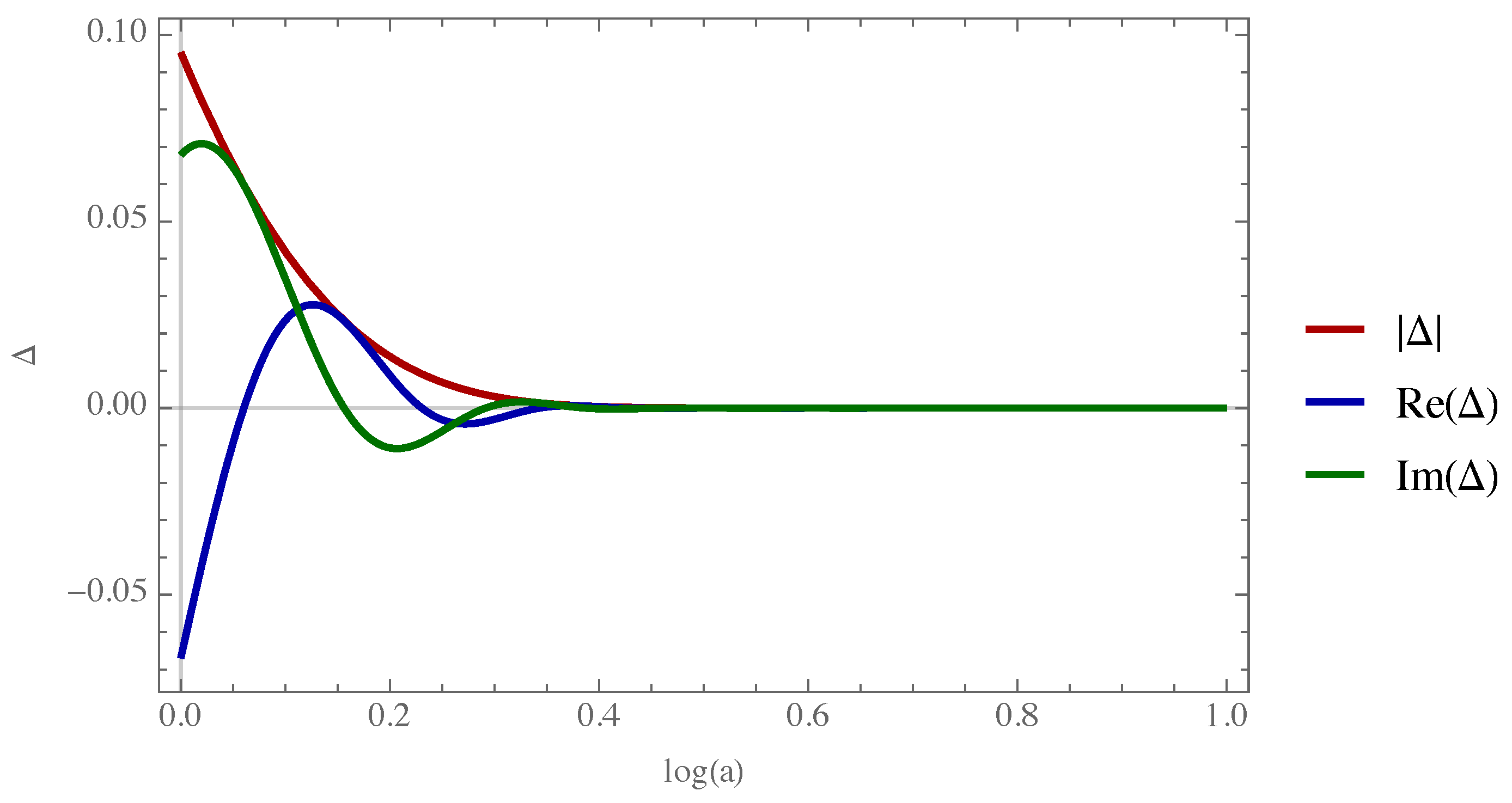
where in the last two terms is the damping factor (analogous to in (17)) that determines the decoherence of the arrows of time as a function of the scale factor a:
where , and we have used for the integral product over the dimensionless index x. Notice also that using the spherical symmetry of the problem, we have . The plot for is shown in Figure 1. The associated decoherence time (time corresponding to a damping factor of ) is of the order of one tenth of the Hubble time:
4. Observation
We consider now the observable effect of the interference of the two arrows of time in the field mode correlations, which would lead to observable results in the power spectrum. We will focus here on a specific mode k and drop all other modes, which are now unobserved, but in principle observable. Besides the problem of measurement, what becomes particularly relevant in quantum cosmology is the problem of the observer: since quantum cosmology is concerned with the total state of the universe, the question arises whether the observer should be included in this state, and if so, what the meaning of the wave function of the universe is. Discussion of this fundamental issue in transposing the tools and concepts of quantum mechanics to the study of the whole universe goes beyond the purpose of the present work, but one comment is in order if we want to discuss the possible effect of the interference. In quantum mechanics one usually implicitly assumes the presence of a classical and external observer behind the scenes, separated from the observed system, as well as from the measuring apparatus and/or the environment. This observer does not “enter the equations” explicitly. Its implied existence may be seen in the derivation of the Tomonaga–Schwinger equation (6), where it can be identified with the three-geometry and survives only in the form of the affine (time) parameter along the local worldline of the “laboratory”. In this sense, one may say that the observer is identified with the laboratory’s spatial geometry and clock. In the ansatz (2), such observers are specified by a single WKB branch, but in the general solution, the observer will be in a superposition of branches. Unlike the one of non-relativistic quantum mechanics, this observer is in principle quantum and is internal to the wavefunctional . The semiclassical approximation then may be seen as analogous to a large mass limit of the observer, which is not affected by the observed system, but can still be found in a quantum superposition of two clocks, each ticking in a different time direction.
While we discuss observation from this tentative point of view, the interpretation of the wavefunctional of the universe and its observer deserves to be considered more accurately, possibly along the lines of a suitable formulation of quantum reference frames (see [23,24,25] or [26,27,28] for recent works) or other relational approaches to quantum observations. Furthermore, works on the concept of “evolution without evolution” such as outlined in [29,30] may be of help in clarifying the issue with reference to the emergence of time. As far as we are concerned here, with what seems a natural extension from the non-relativistic case to the cosmological case, we identify the observer with what we previously referred to as the “system” and take it to be in the superposition (13). The state of the observable matter field for such an observer, up to a proper normalization constant , is obtained by projecting over such superposition, i.e.,
The expectation value for the correlations of a given field mode is then given by two contribution, , where:
is the usual contribution from the terms that survive decoherence, while:
is the contribution coming from the interference of the arrows of time. The normalization constant for the diagonal elements of associated with a given value of scale factor is:
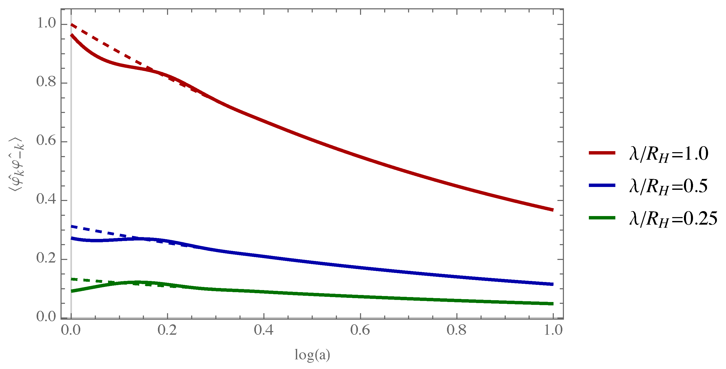
which gives normalized correlations (Figure 2):
Using and therefore , the probability distribution for the outcome of measurement of the power spectrum is given simply by:
which describes how the interference between arrows of time is expected to affect the usual power spectrum outcome distribution (the first term in (42)) at very early times (that is, early compared to the Hubble time).
In order to study the effect of the interference, we have considered only two arrows of time, one inverse to the other, although in general, the geometry will be described by a superposition of wavefronts in the early epoch, depending on the model. In such a general case, the manifestation of the interference will be expectedly more complex, but generally still observable.
Considering the possible observation of this interference in the early universe, in principle, we might look for its trace in the power spectrum of the scalar modes of primordial gravitational waves emitted within a time scale comparable with the Hubble time of the inflationary epoch. The detailed treatment of these observable aspects in the early cosmological scenario, as well as the extension to tensorial perturbations lies beyond the modest intentions of the present work, but the effect on the power spectrum is expected to be very strongly damped as a function of the e-folding . In particular, the relative amplitude is bounded from above as:
At the Hubble time, , and we have already .
5. Conclusions
We have discussed the interference of two different orientations for the cosmological arrow of time identified in the expanding and contracting modes of a de Sitter universe in the semiclassical approximation of the Wheeler–DeWitt equation, as well as their decoherence due to quantum fluctuations of a massless scalar vacuum subject to gravitational particle production. In principle, the interference of the expanding and contracting modes could be observed in the field mode correlations and power spectrum at very early times before the decoherence becomes strong. Whether this simple model can be applied to the inflationary de Sitter phase of our universe or other scenarios where the interference of geometries comes into play is left as a question for future inquiries. We have provided a tentative reason for identifying the observer with the spatial geometry, and therefore, the decoherence refers to the decoherence of the observer itself, which is coupled to the scalar vacuum. In any case, besides the details of the decoherence mechanism, a better understanding of the role of the observer in quantum cosmology in future works is auspicated.
Author Contributions
Both authors contributed equally to this work. Both authors have read and approved the final manuscript.
Funding
Y.N. was supported in part by JSPS KAKENHI Grant No. 15K05073.
Acknowledgments
M.R. gratefully acknowledges support from the Ministry of Education, Culture, Sports, Science and Technology (MEXT) of Japan.
Conflicts of Interest
The authors declare no conflict of interest.
References
- DeWitt, B.S. Quantum gravity. I. The canonical theory. Phys. Rev. 1967, 160, 1113–1148. [Google Scholar] [CrossRef]
- DeWitt-Morette, C. The Pursuit of Quantum Gravity: Memoirs of Bryce DeWitt from 1946 to 2004; Springer: Berlin/Heidelberg, Germany, 2011. [Google Scholar]
- Rovelli, C. The strange equation of quantum gravity. Class. Quantum Grav. 2015, 32, 124005. [Google Scholar] [CrossRef] [Green Version]
- Rovelli, C. Quantum Gravity; Cambridge University Press: Cambridge, UK, 2004. [Google Scholar]
- Hartle, J.; Hawking, S. Wave function of the Universe. Phys. Rev. D 1983, 28, 2960–2975. [Google Scholar] [CrossRef]
- Vilenkin, A. Boundary conditions in quantum cosmology. Phys. Rev. D 1986, 33, 3560–3569. [Google Scholar] [CrossRef]
- Peres, A. On Cauchy’s problem in General Relativity. Nuovo Cimento 1962, 26, 53. [Google Scholar] [CrossRef]
- Kiefer, C. The semiclassical approximation to quantum gravity. In Canonical Gravity: From Classical to Quantum; Ehlers, J., Friedrich, H., Eds.; Springer: Berlin/Heidelberg, Germany, 1994. [Google Scholar]
- Zeh, H.D. The Physical Basis of the Direction of Time, 5th ed.; Springer: Berlin/Heidelberg, Germany, 2007. [Google Scholar]
- Halliwell, J.J.; Perez-Mercader, J.; Zurek, W.H. Physical Origins of Time Asymmetry; Cambridge University Press: Cambridge, UK, 1992. [Google Scholar]
- Zeh, H.D. Emergence of classical time from a universal wavefunction. Phys. Lett. A 1986, 116, 9–12. [Google Scholar] [CrossRef]
- Keifer, C. Continuous measurement of mini-superspace variables by higher multipoles. Class. Quantum Grav. 1987, 4, 1369–1382. [Google Scholar] [CrossRef]
- Keifer, C. Continuous measurement of intrinsic time by fermions. Class. Quantum Grav. 1989, 6, 561–566. [Google Scholar] [CrossRef]
- Halliwell, J.J. Decoherence in quantum cosmology. Phys. Rev. D 1989, 39, 2912–2923. [Google Scholar] [CrossRef]
- Kiefer, C. Decoherence in Quantum Cosmology. In Proceedings of the 10th Seminar on Relativistic Astrophysics and Gravitation, Potsdam, Germany, 21–26 October 1992. [Google Scholar]
- Birrell, N.D.; Davies, P.C.W. Quantum Fields in Curved Space; Cambridge University Press: Cambridge, UK, 1982. [Google Scholar]
- Tsamis, N.C.; Woodard, R.P. The factor ordering problem must be regulated. Phys. Rev. D 1987, 36, 3641–3650. [Google Scholar] [CrossRef]
- Lapchinsky, V.G.; Rubakov, V.A. Canonical quantization of gravity and quantum field theory in curved space-time. Acta Phys. Pol. B 1979, 10, 1041–1048. [Google Scholar]
- Erich, J.; Zeh, H.D.; Kiefer, C.; Giulini, D.J.W.; Kupsch, J.; Stamatescu, I.-O. Decoherence and the Appearance of a Classical World in Quantum Theory, 2nd ed.; Springer: Berlin/Heidelberg, Germany, 2003. [Google Scholar]
- Zurek, W.H. Decoherence and the Transition from Quantum to Classical. Phys. Today 1991, 44, 36–44. [Google Scholar] [CrossRef]
- Paz, J.P.; Zurek, W.H. Environment-induced decoherence, classicality, and consistency of quantum histories. Phys. Rev. D 1993, 48, 2728–2738. [Google Scholar] [CrossRef] [Green Version]
- Schlosshauer, M.A. Decoherence and the Quantum-To-Classical Transition, 1st ed.; Springer: Berlin/Heidelberg, Germany, 2007. [Google Scholar]
- Aharonov, Y.; Susskind, L. Charge superselection rule. Phys. Rev. 1967, 155, 1428–1431. [Google Scholar] [CrossRef]
- Aharonov, Y.; Susskind, L. Observability of the sign change of spinors under 2π rotations. Phys. Rev. 1967, 158, 1237–1238. [Google Scholar] [CrossRef]
- Aharonov, Y.; Kaufherr, T. Quantum frames of reference. Phys. Rev. D 1984, 30, 368–385. [Google Scholar] [CrossRef]
- Angelo, R.M.; Brunner, N.; Popescu, S.; Short, A.; Skrzypczyk, P. Physics within a quantum reference frame. J. Phys. A 2011, 44, 145304. [Google Scholar] [CrossRef]
- Angelo, R.M.; Ribeiro, A.D. Kinematics and dynamics in noninertial quantum frames of reference. J. Phys. A 2012, 45, 465306. [Google Scholar] [CrossRef]
- Pereira, S.T.; Angelo, R.M. Galilei covariance and Einstein’s equivalence principle in quantum reference frames. Phys. Rev. A 2015, 91, 022107. [Google Scholar] [CrossRef]
- Page, D.; Wootters, W. Evolution without evolution: Dynamics described by stationary observables. Phys. Rev. D 1983, 27, 2885–2892. [Google Scholar] [CrossRef]
- Giovannetti, V.; Lloyd, S.; Maccone, L. Quantum time. Phys. Rev. D 2015, 92, 045033. [Google Scholar] [CrossRef] [Green Version]
Figure 1.
Plot of the damping factor as a function of the e-folding .

Figure 2.
Plot of the field mode correlations for different values of length scales (in units of Hubble radius) as a function of the e-folding (i.e., time in units of Hubble time), superposed on their usual value when interference is not taken into account.
Figure 2.
Plot of the field mode correlations for different values of length scales (in units of Hubble radius) as a function of the e-folding (i.e., time in units of Hubble time), superposed on their usual value when interference is not taken into account.

© 2018 by the authors. Licensee MDPI, Basel, Switzerland. This article is an open access article distributed under the terms and conditions of the Creative Commons Attribution (CC BY) license (http://creativecommons.org/licenses/by/4.0/).
Share and Cite
MDPI and ACS Style
Rotondo, M.; Nambu, Y. The Decoherence and Interference of Cosmological Arrows of Time for a de Sitter Universe with Quantum Fluctuations. Universe 2018, 4, 71. https://0-doi-org.brum.beds.ac.uk/10.3390/universe4060071
AMA Style
Rotondo M, Nambu Y. The Decoherence and Interference of Cosmological Arrows of Time for a de Sitter Universe with Quantum Fluctuations. Universe. 2018; 4(6):71. https://0-doi-org.brum.beds.ac.uk/10.3390/universe4060071
Chicago/Turabian StyleRotondo, Marcello, and Yasusada Nambu. 2018. "The Decoherence and Interference of Cosmological Arrows of Time for a de Sitter Universe with Quantum Fluctuations" Universe 4, no. 6: 71. https://0-doi-org.brum.beds.ac.uk/10.3390/universe4060071
Note that from the first issue of 2016, this journal uses article numbers instead of page numbers. See further details here.