Anti-Newtonian Expansions and the Functional Renormalization Group

Abstract

Anti-Newtonian expansions are introduced for scalar quantum field theories and classical gravity. They expand around a limiting theory that evolves only in time while the spatial points are dynamically decoupled. Higher orders of the expansion re-introduce spatial interactions and produce overlapping lightcones from the limiting isolated world line evolution. In scalar quantum field theories, the limiting system consists of copies of a self-interacting quantum mechanical system. In a spatially discretized setting, a nonlinear “graph transform” arises that produces an in principle exact solution of the Functional Renormalization Group for the Legendre effective action. The quantum mechanical input data can be prepared from its $1+0$ dimensional counterpart. In Einstein gravity, the anti-Newtonian limit has no dynamical spatial gradients, yet remains fully diffeomorphism invariant and propagates the original number of degrees of freedom. A canonical transformation (trivialization map) is constructed, in powers of a fractional inverse of Newton’s constant, that maps the ADM action into its anti-Newtonian limit. We outline the prospects of an associated trivializing flow in the quantum theory.

1. Anti-Newtonian Expansions

Non-perturbative techniques come in many guises (as do non-elephants). Non-perturbative series expansions often use an artificial control parameter (number of flavors) and are not applicable to pure gravity or single flavor systems. Moreover, they remain at best asymptotic expansions. The Functional Renormalization Group (FRG) uses a more physical covariant mode modulation parameter and—significantly—is applicable to pure gravity [1,2]. Nevertheless, the FRG—as currently used—also has certain weaknesses: (i) State space positivity is not addressed and no systematic strategy of doing so is known. Most computations are based on Euclidean signature, including those in a foliated setting. This is unproblematic in flat space quantum field theories but not so in curved spacetimes, where a satisfactory notion of “Wick rotation” remains elusive [3]. In quantum gravity, this is compounded with the conformal factor instability. (ii) The Legendre effective action $\Gamma$ is a highly nonlocal functional of the mean fields and no structural characterization of the terms that can occur is known. Hence, the truncation ansätze employed in solving the FRG also lack a clear ordering principle. No statements about asymptotic correctness or convergence of some sequence of truncations are known. (iii) The FRG in itself is kinematical in nature; dynamical information is injected solely through initial conditions. The standard choice is to identify the effective action with the bare action at some UV scale, ${\Gamma }_{{\Lambda }_{\mathrm{UV}}}=S_{\mathrm{bare}}$. In practice, no independent UV regularization is introduced. This blurs the relation to an underlying functional integral and renders the computation of the unstable manifold problematic. When the bare action is identified with the classical action, one arguably makes implicit reference to perturbation theory.

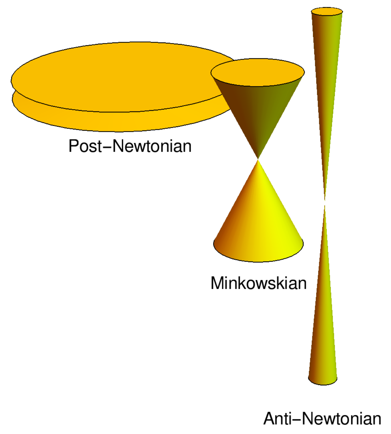
The goal of this note is to show that the FRG can be used differently and combined with a novel non-perturbative series expansion, dubbed anti-Newtonian expansion. Schematically, one expands around a limiting theory that evolves only in time while the spatial points are dynamically decoupled. No Wick rotation is ever performed, time is left real and continuous. The control parameter of the expansion is the spatial interaction range. As such, the expansion is applicable to single flavor systems and to gravity. The natural setting is that of foliated pseudo-Riemannian manifolds. The expansion parameter $\check{\kappa }$ is essentially the inverse scale of the spatial metric ${\mathrm{g}}_{ab}$ and may initially be introduced through the rescaling ${\mathrm{g}}_{ab}\mapsto {\check{\kappa }}^{-1}{\mathrm{g}}_{ab}$. For small $\check{\kappa }$, spacelike distances are relatively enhanced and the lightcones appear to be “squeezed” to almost lines. Each order in the expansion in powers of $\check{\kappa }$ extends the spatial interaction range and eventually restores, or rather defines, the full lightcone structure. In general relativity, the post-Newtonian expansion does roughly the opposite (see Figure 1).

The implementation of such an expansion will depend on the theory considered. In the following, we describe two main cases: a scalar self-interacting quantum field theory on a Friedmann–Lemaître background and classical Einstein gravity coupled to a self-interacting scalar. The latter can be thought of providing generic self-consistent backgrounds for the former, i.e., ones where classical backreaction effects are taken into account. We begin with a brief overview for both settings. More specific accounts are given in later sections.

Reduction of QFT to QM. For a relativistic scalar Quantum Field.

Theory (QFT), the anti-Newtonian expansion entails a reduction of QFT to Quantum Mechanics (QM). The QFT is modeled as a collection of self-interacting QM systems evolving in real continuous time; one such system is associated to each spatial point. A QM system influences its spatial neighbors and the expansion is essentially a spatial gradient expansion. As such, it is applicable to quantum fields on any globally hyperbolic manifold. For now, we restrict attention to globally hyperbolic manifolds which admit flat spatial sections $\Sigma$. These include some prominent relativistic spacetimes such as flat Friedmann–Lemaître or Bianchi I cosmologies and the Schwarzschild solution. Flat spatial sections allow for a straightforward discretization on a hypercubic lattice, also denoted by $\Sigma ={\left(a_s\mathbb{Z}\right)}^d$. The basic action then decomposes into a spatially ultralocal term (a sum of self-interacting $1+0$ dim. actions, one per spatial point) and a hopping term linking nearest neighbors on the lattice with spacing $a_s$

$$\begin{array}{c}\hfill S\left[\varphi \right]=\sum _{x\in \Sigma }s\left[a_s^{d/2}\varphi (·,x)\right]+\check{\kappa }\mathcal{V}\left[\varphi \right].\end{array}$$

(1)

Here, $\varphi ={\varphi }^{\dim }$ is dimensionful and $a_s^{d/2}\varphi$ has length dimension $1/2$. We write $\check{\kappa }$ for the hopping parameter to distinguish it from its counterpart in a fully dimensionless formation. For a Friedmann–Lemaître background, the single site action $s\left[\phi \right]$ and the hopping term $\mathcal{V}\left[\varphi \right]$ are defined as

$$\begin{array}{ccc}s\left[\phi \right]\hfill & :=\hfill & {\int }_{t_i}^{t_f}dt\left\{\frac{1}{2n}{\left({\partial }_t\phi \right)}^2-\frac{1}{2}n{a}^{2d-2}\frac{2d}{a_s^2}{\phi }^2-n{a}^{2d}[U\left(\phi \right)+\Lambda ]\right\}\left(t\right),\hfill \\ \mathcal{V}\left[\varphi \right]\hfill & :=\hfill & \frac{a_s^{d-2}}{2}{\int }_{t_i}^{t_f}dtn\left(t\right)a{\left(t\right)}^{2d-2}\sum _{x,y}\varphi (t,x){\ell }_{xy}\varphi (t,y).\hfill \end{array}$$

(2)

The scale factor $a\left(t\right)$ refers to the line element $d{s}^2=-N{\left(t\right)}^{2}d{t}^2+a{\left(t\right)}^{2}d{x}^a{\delta }_{ab}d{x}^b$ and $n\left(t\right)=N\left(t\right)/a{\left(t\right)}^d$ replaces the lapse $N\left(t\right)$. The single site function $s\left[\phi \right]$, $\phi =\phi \left(t\right)$, can be viewed as the action of a quantum mechanical system. The functional integral based on Equation (1) comes with an ab-initio ultraviolet regularization and is well-defined whenever the quantum mechanical one is. Correlation functions or their generating functionals can be computed by expanding in powers of the hopping term. Such expansions are also known as linked cluster expansions (LCE) and often have a finite radius of convergence. The anti-Newtonian expansion in this setting amounts to a spatial variant of a LCE. The evaluation of some correlation function is reduced to a combinatorial and a QM problem. The combinatorial problem amounts to classifying all possible identifications of spatial sites such that at single sites the spatially ultralocal part of the functional measure produces a quantum mechanical correlation function. This combinatorial problem turns out to have a largely model-independent solution in terms of graph theoretical data. The model-dependent part of the problem consists of the evaluation of the QM correlation functions. We repeat that this strategy avoids issues with Wick rotation or temporal discretization in the functional integral, which is problematic or cumbersome in non-static backgrounds. The QM data will of course have to be provided by techniques other than the path integral.

In fact, this is one of the uses of the FRG in this framework. Many of the subtleties related to regularization or renormalization are simpler or absent in QM. The FRG operates directly on the level of a (quantum mechanical) generating functional, while conventional numerical techniques cannot easily keep track of dependencies on an external (source or mean) field.

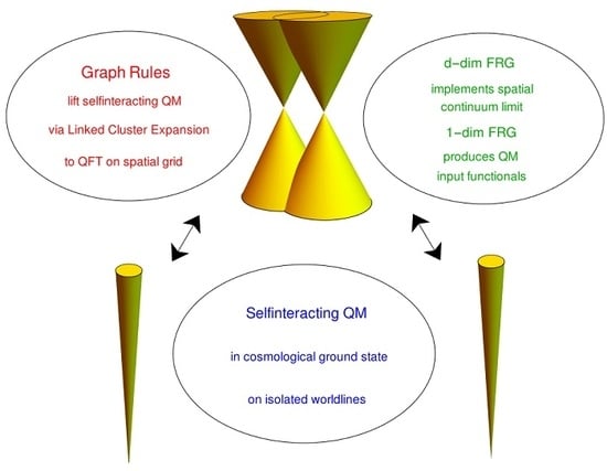
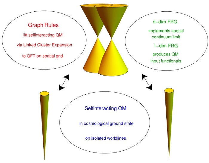
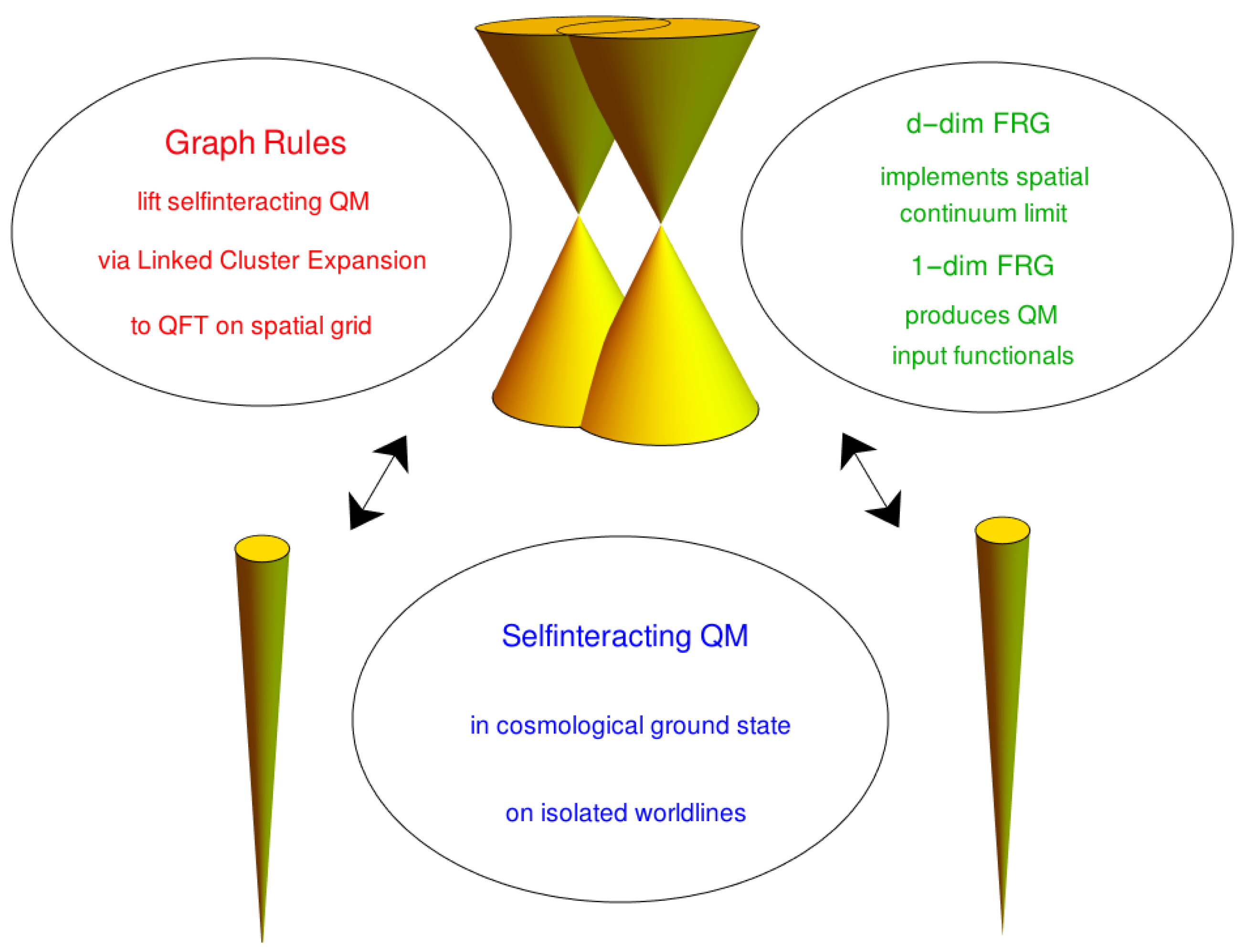
The second use of the FRG lies in the approach to the spatial continuum limit. In similar expansions, the locus of criticality normally coincides with the radius of convergence of the hopping series, which provides a direct if computationally demanding way of determining it [4]. In a Wilsonian framework, the locus of criticality can be characterized as the unstable manifold of an underlying fixed point. As such, it should be computable via the FRG. Indeed, experience with the covariant Euclidean case suggests that the (modified) local potential approximation suffices to determine the locus of criticality. This provides a dramatic simplification, as only a system of ordinary differential equations needs to be solved [5]. Two features appear to underlie this simplification: First, even in the local potential approximation the FRG resums part of the hopping expansion. Second, the initial data injected are the exact single site integrals, which carry the full coupling and ℏ dependence. It is plausible that the spatial continuum limit can similarly be accessed by an FRG based technique. In overview, the programmatic interplay between the FRG and the LCE is shown in Figure 2 for a Friedmann–Lemaître background.

An important step in the program is the formulation of the LCE on the level of the effective action $\Gamma$. The expansion turns out to be coded by abstract graphs to which analytical expressions are assigned via “graph rules”. The graphs and the graph rules are largely model-independent and are summarized in Section 2. Assuming that the finite radius of convergence extends beyond the (modified) local potential approximation, the “graph transform” provides an exact solution of the original FRG.

LCEs have a well defined classical limit governed by tree graphs. This can be used to obtain a graph solution of the classical nonlinear field equations. More interestingly, the classical field equations can be “trivialized” and mapped into the $1+0$ dimensional ones:

$$\frac{\delta S}{\delta \varphi }(\Phi \left[{\varphi }_0\right])=\frac{\delta S_0}{\delta {\varphi }_0}\left({\varphi }_0\right).$$

(3)

Here, $S_0$ is the spatially ultralocal term in Equation (1), thus the right hand side is an ordinary differential equation $\delta s/\delta \phi$, evaluated on $\phi ={\varphi }_0(·,x)$. The map $\Phi \left[{\varphi }_0\right]$ is defined for off-shell configurations ${\varphi }_0$. If so desired, one can specialize to solutions of $\delta s/\delta \phi =0$ to obtain series solutions of the original nonlinear field equation. The map $\Phi \left[{\varphi }_0\right]$ thus reduces the solution of a nonlinear partial differential equation to that of an ordinary differential equation. It admits an expansion in powers of $\check{\kappa }$ such that the lth order ${\Phi }_l\left[{\varphi }_0\right](t,x)$ is a sum of contributions associated with a finite set of tree graphs with l lines. There is a special (“rooted”) vertex labeled by the point $(t,x)$. To each tree graph, a formula is associated according to rules related to the classical limit of those for the quantum LCE of the free energy.

Thus far, the classical background spacetime has been externally prescribed. Upon coupling to classical gravity, one will want the background to be a solution of the Einstein equations sourced by the energy–momentum tensor derived from the matter action. In the case of a Friedmann–Lemaître cosmology, the cosmological scale factor $a\left(t\right)$ will then not be a prescribed function of t but will itself be co-determined by the spatially homogeneous scalar $\phi \left(t\right)$. In other words, even to zeroth order of the spatial gradient expansion a self-consistency condition arises: the $a\left(t\right)$ entering the classical action $S\left[\varphi \right]$ should be such that, for the spatially homogeneous truncation $\varphi (t,x)=\phi \left(t\right)$, the pair $a\left(t\right),\phi \left(t\right)$ solves the coupled ordinary differential equations entailed by the Einstein field equations. This can be built in, essentially by parameterizing the potential $U\left(\varphi \right)$ in terms of a superpotential $\mathrm{u}\left(\varphi \right)$, which in turn arises as the logarithmic derivative of the scale factor $a=a\left(\phi \right)$ viewed as a function of $\phi$.

Reduction of Einstein to Strong Coupling gravity. At subleading orders in the gradient expansion, the coupling to classical gravity will make the spatial inhomogeneities in $\varphi (t,x)$ backreact on the metric. Consequently, the scalar QFT on a homogeneous background such as $d{s}^2=-N{\left(t\right)}^{2}d{t}^2+a{\left(t\right)}^{2}d{x}^a{\delta }_{ab}d{x}^b$ is no longer classically self-consistent. The classical limit of quantum gravity would instead produce a nontrivial spatial metric ${\mathrm{g}}_{ab}(t,x)$ sourced by the energy–momentum tensor of $\varphi (t,x)$. To retain classical self-consistency, a coordinated expansion of Einstein gravity is needed, induced by a decomposition akin to Equation (1). Starting from the $1+d$ decomposition with line element $d{s}^2=-N^{2}d{t}^2+{\mathrm{g}}_{ab}(N^{a}dt+d{x}^a)(N^{b}dt+d{x}^b)$, the appropriate counterpart turns out to be

$$S[\mathrm{g},\varphi ]=S_0[\mathrm{g},\varphi ]+\check{\kappa }\mathcal{V}[\mathrm{g},\varphi ],$$

(4)

where $\check{\kappa }$ enters through a scale transformation and plays the role of a fractional inverse of Newton’s constant (see Section 3). Further,

$$\begin{array}{ccc}{S}_0[q,\phi ]\hfill & =\hfill & \frac{1}{2}{\int }_{t_i}^{t_f}dt{\int }_{\Sigma }dx\left\{\frac{1}{4n}{e}_0\left(q_{ab}\right)G{\left(q\right)}^{ab,cd}{e}_0\left(q_{cd}\right)+\frac{1}{n}{e}_0{\left(\phi \right)}^2-2nq[U\left(\phi \right)+\Lambda ]\right\},\hfill \\ \mathcal{V}[\mathrm{g},\varphi ]\hfill & =\hfill & \frac{1}{2}{\int }_{t_i}^{t_f}dt{\int }_{\Sigma }dxn\mathrm{g}\left\{R\left(\mathrm{g}\right)-{\mathrm{g}}^{ab}{\partial }_a\varphi {\partial }_b\varphi \right\}.\hfill \end{array}$$

(5)

In addition to the propagating fields, the densitized lapse $n=N/\sqrt{\mathrm{g}}$ and the shift $N^a$ enter, the latter only through $e_0:={\partial }_t-{\mathcal{L}}_{\overrightarrow{N}}$, the derivation transversal to the leaves of the foliation. The action $S_0[q,\phi ]$ defines strong coupling gravity, a terminology that is justified below. Its propagating fields are denoted by separate symbols: $q_{ab}$ for the spatial metric and $\phi$ for the scalar. The deWitt metric reads $2G{\left(q\right)}^{ab,cd}=q^{ad}{q}^{bc}+q^{ac}{q}^{bd}-2q^{ab}{q}^{cd}$. The second term $\mathcal{V}$ contains the dynamical spatial gradients, with $R\left(\mathrm{g}\right)$ the Ricci scalar of the spatial metric. The scalar field from Equation (1) has been rendered dimensionless by the rescaling $\varphi =\sqrt{\kappa }{\varphi }^{\dim }$ and the coordinates are also viewed as dimensionless. Identifying $a_s^{(d-1)/2}{\varphi }^{\dim }$ with $\sqrt{\kappa }{\varphi }^{\dim }$ the pure matter part of Equation (4) precisely reduces to the continuum version of Equation (1).

The gravitational counterpart of the tree level trivialization in Equation (3) would similarly map the full into the limiting equations of motion. When the $q_{ab},\phi$ “seeds” are on-shell, series solutions of the Einstein equations arise. A similar framework is known as the “relativistic gradient expansion” and relates to themes such as “separate universe”, “asymptotic silence”, “asymptotic velocity domination”, “resummation of secular terms”, etc.. In the gravitational counterpart of Equation (3), the field equations of course include the constraints. Consequently, the relativistic gradient expansion only applies to on-shell seeds. For off-shell seed configurations $q_{ab},\phi$, the constraints would no longer be preserved from one time slice to the next. Consequently, the gravitational version of Equation (3) is feasible only if the right hand side is set to zero.

Remarkably, in a Hamiltonian formulation, a stronger variant of Equation (3) can consistently be imposed for off-shell seeds and maps the full into the limiting action

$$S_{\check{\kappa }}\left[{{\rm Y}}_{\check{\kappa }}(q,p,\phi ,p^{\phi })\right]=S_0[q,p,\phi ,p^{\phi }].$$

(6)

Here, $S_{\check{\kappa }}[\mathrm{g},\wp ,\varphi ,p^{\varphi }]$ and $S_0[q,p,\phi ,p^{\phi }]$ are the Hamiltonian versions of S and $S_0$ in Equations (4) and (5), respectively. The map ${{\rm Y}}_{\check{\kappa }}$ is a canonical transformation and can be constructed iteratively as a series in $\check{\kappa }$ merely by solving ordinary differential equations. The successful implementation of Equation (6) turns out to also imply the counterpart of Equation (3) for the Hamiltonian fields equations, but now without troubles from constraint non-propagation.

2. Linked Cluster Expansions and FRG

Starting from the scalar action in Equation (1), a mode-modulation term quadratic in $\varphi$ could be added and the Wetterich equation for the effective average action be derived along the usual lines [1,2,4]. Since the hopping term $\mathcal{V}$ is already quadratic in $\varphi$, one can directly take $\check{\kappa }$ as the control parameter and derive a FRG in $\check{\kappa }$ for the (modified) Legendre effective action $\Gamma$. For Euclidean signature on a hypercubic lattice, no complications arise. Since $\mathcal{V}$ in Equation (2) contains fields at the same time, one will initially replace it by a temporally point split version $\check{\mathcal{V}}$ with kernel $\check{\ell }(t,x;t^{\prime },x^{\prime })$. The resulting “hopping” FRG reads

$${\partial }_{\check{\kappa }}\Gamma \left[\varphi \right]=\frac{i\hslash }{2}{a}_s^{d-2}\sum _{x,y\in {\left(a_s\mathbb{Z}\right)}^d}\int d\nu \left(t\right)d\nu \left(s\right)\check{\ell }(t,x;s,y){[{\Gamma }^{\left(2\right)}\left(\varphi \right)+\check{\kappa }\check{\ell }]}^{-1}(t,x;s,y),$$

(7)

where we write $d\nu \left(t\right)=dtn\left(t\right)a{\left(t\right)}^{2d-2}$ for the reparameterization invariant temporal measure. The main deviation from the standard uses is that initial conditions are imposed at the ultralocal scale

$$\Gamma \left[\varphi \right]{|}_{\check{\kappa }=0}\stackrel{{\displaystyle !}}{=}{\Gamma }_0\left[\varphi \right]=\sum _{x\in {\left(a_s\mathbb{Z}\right)}^d}\gamma \left[a_s^{d/2}\varphi (·,x)\right].$$

(8)

Here, $\gamma \left[\phi \right]$ is the QM effective action for $s\left[\phi \right]$ in Equation (2), which at the moment we assume to be known. Once a solution of Equation (7) was known, the replacement of $\check{\ell }$ with some scale dependent mode modulator $R_k(t,x;t^{\prime },x)$ would produce a solution of the (spatially discretized) Wetterich equation in $1+d$ form, ${\Gamma }_k{=\Gamma |}_{\check{\kappa }\check{\ell }\to R_k}$.

As usual, one will not be able to solve Equation (7) in closed form. A power series ansatz

$$\Gamma \left[\varphi \right]=\sum _{l=0}^{\infty }\frac{{\check{\kappa }}^l}{l!}{\Gamma }_l\left[\varphi \right],$$

(9)

converts Equation (7) into a closed recursion for the ${\Gamma }_l$, $l\ge 1$, with initial data in Equation (8). Further, each ${\Gamma }_l$ can be shown to have a well-defined coincidence limit as the original hopping term is restored, $\check{\ell }(t,x;t^{\prime },x^{\prime })\to {\ell }_{x{x}^{\prime }}\delta (t-t^{\prime })n{\left(t\right)}^{-1}a{\left(t\right)}^{-2d+2}$. This also restores the exact—not mode-modulated—QM dynamics. By direct iteration, one finds ${\Gamma }_1\left[\varphi \right]=0$ and

$$\begin{array}{ccc}{\Gamma }_2\left[\varphi \right]\hfill & =\hfill & a_s^{-4}\int d\nu \left(t_1\right)d\nu \left(t_2\right)\frac{i\hslash }{2}\sum _{x_1,x_2}{\left({\ell }_{x_1{x}_2}\right)}^2{\varpi }_2(t_1,t_2|x_1){\varpi }_2(t_2,t_1|x_2),\hfill \\ {\Gamma }_3\left[\varphi \right]\hfill & =\hfill & -a_s^{-6}\int d\nu \left(t_1\right)d\nu \left(t_2\right)d\nu \left(t_3\right)\{\frac{{(i\hslash )}^2}{2}\sum _{x_1,x_2}{\left({\ell }_{x_1{x}_2}\right)}^3{\varpi }_3(t_1,t_2,t_3|x_1){\varpi }_3(t_1,t_2,t_3|x_2)\hfill \\ & +\hfill & i\hslash \sum _{x_1,x_2,x_3}{\ell }_{x_1{x}_2}{\ell }_{x_2{x}_3}{\ell }_{x_3{x}_1}{\varpi }_2(t_1,t_2|x_1){\varpi }_2(t_2,t_3|x_2){\varpi }_2(t_3,t_1|x_3)\}.\hfill \end{array}$$

(10)

$$\begin{array}{c}{\Gamma }_4\left[\varphi \right]=a_s^{-8}\int d\nu \left(t_1\right)d\nu \left(t_2\right)d\nu \left(t_3\right)d\nu \left(t_4\right)\{\hfill \\ \frac{{(i\hslash )}^3}{2}\sum _{x_1,x_2}{\left({\ell }_{x_1{x}_2}\right)}^4{\varpi }_4(t_1,t_2,t_3,t_4|x_1){\varpi }_4(t_1,t_2,t_3,t_4|x_2)\hfill \\ +6{(i\hslash )}^2\sum _{x_1,x_2,x_3}{\left({\ell }_{x_1{x}_2}\right)}^2{\ell }_{x_1{x}_3}{\ell }_{x_2{x}_3}{\varpi }_3(t_1,t_2,t_3|x_1){\varpi }_3(t_1,t_2,t_4|x_2){\varpi }_2(t_3,t_4|x_3)\hfill \\ +3{(i\hslash )}^2\sum _{x_1,x_2,x_3}{\left({\ell }_{x_1{x}_2}\right)}^2{\left({\ell }_{x_2{x}_3}\right)}^2{\varpi }_2(t_1,t_2|x_1){\varpi }_2(t_3,t_4|x_3){\mu }_v(t_1,t_2,t_3,t_4|x_2)\hfill \\ +3i\hslash \sum _{x_1,x_2,x_3,x_4}{\ell }_{x_1{x}_2}{\ell }_{x_2{x}_3}{\ell }_{x_3{x}_4}{\ell }_{x_4{x}_1}{\varpi }_2(t_1,t_2|x_1){\varpi }_2(t_2,t_3|x_2){\varpi }_2(t_3,t_4|x_3)){\varpi }_2(t_4,t_1|x_4)\},\hfill \end{array}$$

(11a)

$$\begin{array}{c}{\mu }_v(t_1,t_2,t_3,t_4|x_2)={\varpi }_4(t_1,t_2,t_3,t_4|v)\hfill \\ -\int a{\left(s_1\right)}^{2}d\nu \left(s_1\right)a{\left(s_2\right)}^{2}d\nu \left(s_2\right){\varpi }_3(t_1,t_2,s_1|v){\gamma }_2(s_1,s_2|v){\omega }_3(s_2,t_3,t_4|v).\hfill \end{array}$$

(11b)

In addition to the QM vertex functions ${\gamma }_n$, their connected counterparts ${\varpi }_n$ enter. Explicitly, introducing the QM free energy via $\omega \left[j\right]:=\int dt\phi \left[j\right]\left(t\right)j\left(t\right)-\gamma \left[\phi \right]$, $(\delta \gamma /\delta \phi )\left(\phi \right[j\left]\right)=j$, we define for $n\ge 2$

$$\begin{array}{c}{\varpi }_n(t_n,\dots ,t_1|x):=\frac{{\delta }^n\omega \left[j\right]}{\delta j\left(t_n\right)\dots \delta j\left(t_1\right)}{|}_{j(·)\mapsto a_s^{d/2}\frac{\partial \gamma }{\partial \phi }\left(a_s^{d/2}\varphi (·,x)\right)},\hfill \\ {\gamma }_n(t_n,\dots ,t_1|x):=\frac{{\delta }^n\gamma }{\delta \phi \left(t_n\right)\dots \delta \phi \left(t_1\right)}{|}_{\phi (·)\mapsto a_s^{d/2}\varphi (·,x)}.\hfill \end{array}$$

(12)

These transform as scalars under temporal reparameterizations for fixed x. For $n=1$, we identify ${\varpi }_1\left(t\right|x)$ with $a_s^{d/2}\varphi (t,x)$ and ${\gamma }_1\left(t\right|x)$ with $j\left[\phi \right](t,x)$.

The direct solution of the recursion quickly becomes impractical, both manually and by computer. Instead, a graph theoretical approach was developed in [6] and leads to a closed formula for ${\Gamma }_l\left[\varphi \right]$ (without having to work out the lower orders first). A graph $L=(V,E)$ comprises a set of vertices V, a set of edges (or lines) E, and the information that pairs of vertices are connected by (possibly several) edges. The graphs occurring are not Feynman diagrams: the lines are not directed, and even for a polynomial interaction there is no bound on the number of lines incident to a vertex or on the number of lines connecting a pair of vertices. All graphs occurring are one-line irreducible (1LI), that is, they are connected and remain so if any one line is cut. In only that sense are they analogous to the 1PI graphs occurring in the perturbative evaluation of $\Gamma$. In the LCE, the lth order, ${\Gamma }_l\left[\varphi \right]$, is expressed as a finite sum of contributions from 1LI graphs with $l=\left|E\right|$ lines. To each such graph, a formula is assigned according to certain “graph rules”. In particular, each contribution is weighed with the inverse of the symmetry factor of the graph. A line connecting vertices $i,j$ always has $-{\ell }_{ij}/a_s^2$ assigned. The formula assigned to vertices depends on the whether or not the graph falls apart upon removal of the vertex. If it does not, a single term (essentially some ${\varpi }_n$) is assigned to it. If the graph does fall apart upon removal of the vertex, the vertex is called an articulation point. In that case, a sum of convolution integrals in products of ${\varpi }_n$ and ${\gamma }_n$’s is assigned to the vertex according to a separate “dashed graph rule” involving only labeled tree graphs (with dashed lines for contradistinction).

The gist of the construction can be illustrated with ${\Gamma }_4$. There are four 1LI graphs contributing, only one of which contains an articulation point marked with v:

(13)

The weight associated with v is a contribution of two labeled dashed tree graphs

(14)

The labels arise from set partitions of the blocks b attached to v, in this case two copies of $b=$ . The symmetry factors now arise from a combination of those of the unlabeled tree graph and the labeling sets, and in Equation (14) just equal 2 for both graphs. The “dashed graph rule” applied to Equation (14) then reproduces ${\mu }_v$ in Equation (11b). Inserted into Equation (13), the application of the main graph rule reproduces Equation (11a). This structure generalizes: there is a “main graph rule” that produces ${\Gamma }_l$ up to the weight assignment ${\mu }_v$ for articulation points v; and there is a “dashed graph rule” that provides ${\mu }_v$ from a sum of labeled tree graphs.

Theorem 1

([6]). (Γ graph rule)

For any $l\ge 2$, the solution ${\Gamma }_l\left[\varphi \right]$ of the recursion implied by Equations (7)–(9) is given by the following graph rules:

(a) 

At order $l\ge 2$, draw all topologically distinct 1LI graphs with l edges, $L=(V,E)\in {\mathcal{L}}_l$. Assign a dummy label i to each vertex and dummy label e to each edge.

(b) 

Multiply by $l!{(i\hslash )}^{c\left(L\right)}/\mathrm{Sym}\left(L\right)$, where $\mathrm{Sym}\left(L\right)$ is the symmetry factor of the graph and $c\left(L\right)$ is its cyclomatic number (number of loops).

(c) 

To each graph a weight $\mu \left(L\right)$ is assigned as follows: an edge connecting vertices $i,j$ is attributed a factor $-{\ell }_{ij}/a_s^2$. A vertex i of degree n is attributed a factor ${\mu }_v(e_n,\dots ,e_1|i)$, where $e_1,\dots ,e_n$ are the edges incident on i.

(d) 

Use the separate “dashed graph rule” invoking only labeled tree graphs to obtain ${\mu }_v$. In particular, ${\mu }_v={\varpi }_v$, if v is not an articulation point.

(e) 

Embed the graph into ${\Sigma }^{\left|V\right|}\times {\mathbb{R}}^{\left|E\right|}$ by associating each vertex with a unique spatial lattice point, $i\mapsto x_i\in \Sigma$, $i=1,\dots ,\left|V\right|$; the same lattice point may occur several times. Associate to each edge label a unique real time variable, $e\mapsto t_e\in \mathbb{R}$, $e=1,\dots ,l=\left|E\right|$. Perform an unconstrained sum over all $x_1,x_2,\dots ,x_{\left|V\right|}$ and an unconstrained integration over all $t_1,\dots ,t_l$, with temporal measures $d\nu \left(t_1\right),\dots ,d\nu \left(t_l\right)$.

The “dashed graph rule” producing ${\mu }_v$ in (d) is described in Section 3 of [6] for Euclidean signature QFT on ${\mathbb{Z}}^{1+d}$. It carries over with minor modifications to the spatial LCE at hand. We omit the formulation of the “dashed graph rule” itself and merely highlight the necessary modifications: the ends of the dashed lines ending on open circles are given labels $s_j$. A dashed line with end labels $s_1,s_2$ connecting two open circles is attributed ${\gamma }_2(s_1,s_2|i)$, while a $m\ge 3$ valent dashed vertex is attributed a factor ${\gamma }_m(s_m,\dots ,s_1|i)$. The labeled open circles are attributed factors of the form ${\varpi }_{n+m}(t_n,\dots ,t_1,s_m,\dots ,s_1|i)$, where the $t_1,\dots ,t_n$ are associated with the full edges, and the $s_1,\dots ,s_m$ are associated with the dashed edges. An unconstrained integral is to be performed over the time arguments associated with the dashed edges with temporal measure $a{\left(t\right)}^{2}d\nu \left(t\right)$. Technically the “dashed graph rule” also applies to non-articulation vertices. Then, $\{b_1,\dots ,b_k\}\in ○$ is the only labeled tree graph contributing and the result is just ${\varpi }_n$, with n the total number of edges incident to the vertex from the k blocks.

The simplest nontrivial instance of the “dashed graph” rule applies to Equation (14) and reproduces the recursively computed vertex weight in Equation (11b). There exists an alternative recursion that allows one to isolate the contribution to articulation vertices with a specified structure of incident blocks. The “dashed graph rule” has been tested extensively along these lines.

In combination, the “main” and the “dashed” graph rule give rise to a closed graph formula for ${\Gamma }_l\left[\varphi \right]$ analogous to the one for Euclidean signature [6]. Since it requires more graph theoretical notions and notations, we omit it here and instead highlight a number of structural properties:

• The graph rule is to some extent model-independent. The form of the scalar potential $U\left(\varphi \right)$ does not enter and the embedding of the abstract graphs into (the spatially discretized) spacetime occurs only in Part (e).
• Traditional LCE mostly use connected graphs. The expansion of $\Gamma \left[\varphi \right]$ in terms of one-line-irreducible (1LI) graphs leads to a considerable computational gain as there are far fewer 1LI graphs. For example, for $l=6$, there are 100 connected but only 22 1LI graphs.
• The weights ${\mu }_v$ depend only on the structure of the abstract graph at v, through the pattern of incident subgraphs. As the same patterns reoccur in many 1LI graphs the ${\mu }_v$’s need to be generated only once and can be stored in a look-up table.
• After embedding the graphs into spacetime, the result characterizes $\Gamma$’s nonlocality precisely and to all orders.
• The relation to the underlying FRG Equations (7) and (8) provides options for a resummation, especially for spatially and/or temporally homogeneous configurations.

The last point relates to the benign convergence properties of many LCEs. In particular, for a lattice ${\varphi }_4^4$ theory, the LCE is known to have finite radius of convergence for all susceptibilities [7]. The adaptation to a functional setting and the Friedmann–Lemaître spacetimes is not immediate. However, the functional analytical raison d’être of the benign convergence properties clearly remains valid: the perturbation (quadratic in the field) is Kato bounded by the unperturbed Hamiltonian (more than quadratic in the field). Irrespective of technical details, one may reasonably expect the LCE for $\Gamma$ to have improved convergence properties compared to perturbation theory.

Moreover, the assumption of a finite radius of convergence can be tested for self-consistency using the FRG itself. This is because the hopping FRG allows one to access the unstable manifold of a fixed point underlying continuum behavior. On the other hand, in known cases, the radius of convergence of LCEs coincides with the locus of criticality [4]. Since bulk quantities such as the spin susceptibility are sufficient to determine the radius of convergence, one may take the effective action specialized to (spacetime) homogeneous fields itself as an alternative bulk quantity. In the FRG context, this leads to a hopping variant of the well studied local potential approximation. The variant introduces a scale dependent mode modulation term in the usual way but injects initial data at the ultralocal scale [5,8]. Along these lines the local potential approximation resums the relevant parts of the hopping expansion and allows one to determine the unstable manifold of an underlying fixed point. Compared to the traditional direct way of determining the radius of convergence of the hopping expansion (by pushing the expansion to high orders and extrapolating to infinite order), this provides a dramatic simplification. Concretely, only a set of ordinary differential equations need to be solved via a shooting technique. The strategy has been tested to compute the critical line in lattice ${\varphi }_4^4$ theory [5] and yields good agreement with the Lüscher-Weisz benchmark [9]. The adaptation to the present spatially discretized ${\varphi }_{1+3}^4$ on Friedmann–Lemaître backgrounds introduces several new features and will be reported elsewhere.

3. Kinematical versus Dynamical Gravitational Gradients

As noted after Equation (5), we refer to the gravity theory with action $S_0[q,\phi ]$ as strong coupling gravity. To justify the terminology, we start from the Lagrangian action for Einstein gravity minimally coupled to a self-interacting scalar field ${\varphi }^{\dim }$. Including Newton’s constant $\kappa =c_d{G}_N$, $c_3=8\pi$, the $1+d$ form of the action can be expressed in terms of the functionals in Equation (5) as

$$\frac{1}{\kappa }{S}_0[\mathrm{g},\sqrt{\kappa }{\varphi }^{\dim }]+\frac{1}{\kappa }\mathcal{V}[\mathrm{g},\sqrt{\kappa }{\varphi }^{\dim }].$$

(15)

The rescaled scalar field $\varphi =\sqrt{\kappa }{\varphi }^{\dim }$ is dimensionless and the potential $U\left(\varphi \right)$ in Equation (5) has already been viewed as a function of it. Next, we subject Equation (15) to the following scale transformation

$$\begin{array}{c}\kappa \to {\lambda }^d\kappa ,{\mathrm{g}}_{ab}(t,x)\to {\lambda }^2{\mathrm{g}}_{ab}(t,x)\hfill \\ N\to N,N^a\to N^a,\varphi \to \varphi ,\Lambda \to \Lambda ,\hfill \end{array}$$

(16)

for $\lambda >0$. After the rescaling, we set $\kappa =1$ and rename $\check{\kappa }={\lambda }^{-2}$. This gives Equation (4). The decomposition in Equation (4) separates kinematical spatial gradients carried by $e_0$ from dynamical gradients carried by $R\left(\mathrm{g}\right)$, ${\partial }_a\varphi {\mathrm{g}}^{ab}{\partial }_b\varphi$, and can serve as the starting point for an anti-Newtonian expansion: the $S_0$ term can be viewed as the $\lambda \to \infty$ limit of the rescaled original action. By Equation (16), a large $\lambda \gg 1$ emulates a large Newton constant and also enhances spacelike distances compared to timelike ones. Neighboring world lines are harder to communicate with and the lightcone structure appears anti-Newtonian. It is instructive to absorb $\kappa$ into a dimensionful spatial metric ${\mathrm{g}}_{ab}^{\dim }={\kappa }^{-2/d}{\mathrm{g}}_{ab}$. Then, all fields $N,n^{\dim }=n\kappa ,N^a,\varphi ,{\mathrm{g}}_{ab}^{\dim }$ are invariant under the scale transformation and the action in Equation (15) reads

$$S_0[{\mathrm{g}}^{\dim },\varphi ]+\frac{1}{{\kappa }^{2/d}}\mathcal{V}[{\mathrm{g}}^{\dim },\varphi ].$$

(17)

In this scale invariant field basis, the role of $\check{\kappa }$ is thus played by ${\kappa }^{-2/d}$, and an expansion in powers of $\check{\kappa }$ is literally a strong coupling expansion.

The limiting gravity theory described by $S_0$ has originally been suggested in Hamiltonian form by Isham [10] and was subsequently studied in [11,12,13,14,15]. In vacuum and without cosmological constant, it is equivalent to the “zero-signature” limit of Einstein gravity formulated by Henneaux [16]. In related developments, first order forms of “Carroll gravity” theories have been introduced [17,18], so far of uncertain relation to Henneaux’s version. In a mathematical relativity context, the field equations of $S_0$ are known as the “velocity dominated” field equations. They describe the limiting behavior of a class of “asymptotically velocity dominated” solutions of the Einstein field equations [19,20]. Conversely, “Fuchsian techniques” [21,22,23] allow one to rigorously construct relativistic spacetimes from “seed” solutions of the velocity dominated fields equations.

The relativistic gradient expansion similarly takes seed solutions of the velocity dominated system as a starting point but aims initially at a formal series expansion in powers of some control parameter $ϵ$. Since its early beginnings in the context of the BKL scenario [24,25,26,27], it has been recast as an alternative to (resummed) cosmological perturbation theory, deemed valid on “superhorizon” scales [28,29,30,31,32]. Typically, the temporal gauge is fixed from the outset and a power series ansatz is made for the spatial metric, ${\mathrm{g}}_{ab}=q_{ab}+ϵ{\mathrm{g}}_{ab}^{\left(1\right)}+{ϵ}^2{\mathrm{g}}_{ab}^{\left(2\right)}+O\left({ϵ}^3\right)$. Other gauges require the expansion also of lapse and/or shift. Although introduced differently, the parameter $ϵ$ turns out to play the same role as $\check{\kappa }$ in the field equations of Equation (4). Upon expansion of the rescaled field equations, one obtains a recursive system of linear partial differential equations for the ${\mathrm{g}}_{ab}^{\left(n\right)}$, $n\ge 1$. These include expanded versions of the constraints. For generic seeds, no significant simplification occurs in the constraint analysis compared to the nonlinear case. In practice, one argues that for cosmological purposes seed solutions of the factorized form $q_{ab}(t,x)=a{\left(t\right)}^2{\overline{q}}_{ab}\left(x\right)$ suffice. For such seeds, the recursion relations reduce to systems of linear ordinary differential equations, which to low orders often allow for an explicit integration. There is a streamlined version of the expansion employing the Hamilton–Jacobi method [33,34]. It too is in practice limited to seed solutions of the form $q_{ab}(t,x)=a{\left(t\right)}^2{\overline{q}}_{ab}\left(x\right)$.

The decomposition in Equation (4) is of course valid off-shell, and in order to make contact with the LCE of the matter sector via Equation (3), one would want to keep the seed configurations $q_{ab}(t,x)$ generic and off-shell. This can clearly not be done along the lines of the relativistic gradient expansion, because for off-shell seeds constraint propagation is violated. As mentioned in the Introduction, the appropriate counterpart of Equation (3) for gravity turns out to be Equation (6) in a Hamiltonian formulation. We therefore prepare here the Hamiltonian version of the decomposition in Equation (4). By Legendre transforming Equation (4) or otherwise, one finds

$$\begin{array}{c}{S}_{\check{\kappa }}[\mathrm{g},\wp ,\varphi ,p^{\varphi }]={\int }_{t_1}^{t_2}dt{\int }_{\Sigma }dx\left\{{\wp }^{ab}{\partial }_t{\mathrm{g}}_{ab}+p^{\varphi }{\partial }_t\varphi -N^a{\mathcal{H}}_a-n{\mathcal{H}}_{\check{\kappa }}\right\},\hfill \\ {\mathcal{H}}_{\check{\kappa }}={\mathcal{H}}_0-\check{\kappa }V,{\mathcal{H}}_a=-2{\mathrm{g}}_{ac}{\nabla }_b{\wp }^{cb}-p^{\varphi }{\partial }_a\varphi ,\hfill \\ {\mathcal{H}}_0=2{\wp }^{ab}{\mathrm{g}}_{ac}{\mathrm{g}}_{bd}{\wp }^{cd}-\frac{2}{d-1}{\wp }^2+\frac{1}{2}{\left(p^{\varphi }\right)}^2+\mathrm{g}[U\left(\varphi \right)+\Lambda ],\hfill \\ V=\frac{1}{2}\mathrm{g}R\left(\mathrm{g}\right)-\frac{1}{2}\mathrm{g}{\mathrm{g}}^{ab}{\partial }_a\varphi {\partial }_b\varphi .\hfill \end{array}$$

(18)

Here, ${\wp }^{ab},p^{\varphi }$ are the momenta conjugate to ${\mathrm{g}}_{ab},\varphi$, the $-1$ density lapse n is used as Lagrange multiplier, and ${\mathcal{H}}_{\check{\kappa }}$ correspondingly is a $+2$ spatial density. As indicated, we write $S_{\check{\kappa }}$ for the Hamiltonian action, where $\check{\kappa }$ only occurs in the Hamiltonian constraint ${\mathcal{H}}_{\check{\kappa }}$. The limit $S_0={lim}_{\check{\kappa }\to 0}{S}_{\check{\kappa }}$ defines the Hamiltonian action of strong coupling gravity (and will be distinguishable from the Lagrangian $S_0$ by the context). It will be regarded as a functional of its own set of dynamical variables:

$$\begin{array}{ccc}\hfill S_0[q_{ab},p^{ab},\phi ,p^{\phi }]& =\hfill & {\int }_{t_i}^{t_f}dt{\int }_{\Sigma }dx\left\{p^{ab}{\partial }_t{q}_{ab}+p^{\phi }{\partial }_t\phi -N^a{\mathcal{H}}_{0,a}-n{\mathcal{H}}_0\right\},\hfill \\ \hfill {\mathcal{H}}_{a,0}& =\hfill & -2{\nabla }_b{p}_a^b+p^{\phi }{\partial }_a\phi ,\hfill \\ \hfill {\mathcal{H}}_0& =\hfill & 2p^{ab}{p}_{ab}-\frac{2}{d-1}{p}^2+\frac{1}{2}{\left(p^{\phi }\right)}^2+q[U\left(\phi \right)+\Lambda ].\hfill \end{array}$$

(19)

The evolution equations are best written in terms of $p_a^b:=q_{ac}{p}^{cb}$ and read

$$e_0\left(p_a^b\right)+nq[U\left(\phi \right)+\Lambda ]{\delta }_a^b=0,e_0\left(p^{\phi }\right)+nq{U}^{\prime }\left(\phi \right)=0,$$

(20)

with $U^{\prime }\left(\phi \right)=dU\left(\phi \right)/d\phi$. Along the flow lines of $e_0$, these are ordinary differential equations. Further, ${\mathcal{H}}_0=0$ is an algebraic condition and only ${\mathcal{H}}_{0,a}=0$ remains a partial differential equation. The constraints are preserved under the evolution in Equation (20)

$$e_0\left({\mathcal{H}}_0\right)=0,e_0\left({\mathcal{H}}_a\right)=n^{-1}{\partial }_a\left(n^2{\mathcal{H}}_0\right).$$

(21)

In addition to these design features, strong coupling gravity has several remarkable bonus properties:

• $S_0$ is invariant under the full spatiotemporal diffeomorphism group, but with respect to a non-tensorial realization [13]. It propagates the same number of physical dofs as Einstein gravity.
• The Poisson algebra generated by ${\mathcal{H}}_0,{\mathcal{H}}_{0,a}$ is a Lie algebra (with structure constants instead of functions). As usual, ${\mathcal{H}}_{0,a}$ generates spatial diffemorphisms, but the Hamiltonian constraints commute [10,12].
• The Poisson algebra admits local observables, even in vacuum or with a single scalar field [14].
• Coarse graining of the physical dofs commutes with time evolution and leaves geodesics unaffected [15].

These properties highlight why the successful implementation of Equation (6) would result in a dramatic simplification of precisely those aspects that make gravity so dissimilar from other field theories.

4. Canonical Trivialization of Gravitational Gradients

The construction leading to Equation (6) is best placed in the context of a “trivializing map”, a concept that we recapitulate here for the case of a scalar QFT. In brief, one aims at a field redefinition $\varphi =Y\left[{\varphi }_0\right]$ that trivializes the functional measure but reproduces the exact correlation functions:

$${〈\varphi \left(x_1\right)\dots \varphi \left(x_n\right)〉}_{\mathrm{exact}}\stackrel{{\displaystyle !}}{=}{〈Y\left[{\varphi }_0\right]\left(x_1\right)\dots Y\left[{\varphi }_0\right]\left(x_n\right)〉}_{\mathrm{free}/\mathrm{simple}}.$$

(22)

On the left hand side, the correlation functions are assumed to be realized in terms of a regularized Lorentzian signature functional integral with action $S_{\check{\kappa }}\left[\varphi \right]$. On the right hand side, the functional integral is taken with respect to a target measure set by a free or otherwise simplified action $S_0\left[{\varphi }_0\right]$. We may assume the coupling constant $\check{\kappa }$ to be chosen such that $S_{\check{\kappa }}{\left[\varphi \right]|}_{\check{\kappa }=0}=S_0\left[\varphi \right]$. In terms of the generating functional, the condition in Equation (22) amounts to

$$\int d\mu \left(\varphi \right)exp\left\{\frac{i}{\hslash }{S}_{\check{\kappa }}\left[\varphi \right]+J·\varphi \right\}\stackrel{{\displaystyle !}}{=}\int d\mu \left({\varphi }_0\right)exp\left\{\frac{i}{\hslash }{S}_0\left[{\varphi }_0\right]+J·Y_{\check{\kappa },\hslash }\left[{\varphi }_0\right]\right\},$$

(23)

with “$·$’ indicating a spacetime integral/sum. A sufficient condition is

$$S_{\check{\kappa }}\left[Y_{\check{\kappa },\hslash }\left[{\varphi }_0\right]\right]+\frac{\hslash }{i}ln\mathrm{Det}\frac{\delta Y_{\check{\kappa },\hslash }\left[{\varphi }_0\right]}{\delta {\varphi }_0}\stackrel{{\displaystyle !}}{=}{S}_0\left[{\varphi }_0\right]+\mathrm{const},$$

(24)

where we indicate the parametric dependence of Y on $\check{\kappa }$ and ℏ. For finite dimensional measures, such maps must exist on general grounds. For relativistic QFTs, their investigation began only recently. The key results are: (i) Trivializing maps exist when the target measure is free ($S_0$ quadratic in the fields) for all standard flat space QFTs, including gauge theories [35]. The maps are constructed perturbatively to all orders in the coupling constant and the signature is inessential. (ii) For Euclidean lattice Yang–Mills theories [36] and nonlinear sigma-models [37], exact trivializing maps exist on functional analytic grounds that reduce the full to the strong coupling measure. The maps can again be constructed iteratively (in powers of the inverse coupling) to all orders. (iii) An important tool is the “trivializing flow”. Instead of trying to construct solutions to Equation (24) directly, one aims at finding a functional gradient flow that characterizes it

$${\partial }_{\check{\kappa }}{Y}_{\check{\kappa },\hslash }=\frac{\delta {\Omega }_{\check{\kappa },\hslash }}{\delta \varphi }\left(Y_{\check{\kappa },\hslash }\right)\mathrm{with}{\Omega }_{\check{\kappa },\hslash }\mathrm{to}\mathrm{be}\mathrm{found}.$$

(25)

Differentiating Equation (24) with respect to $\check{\kappa }$ leads to a functional Schrödinger equation for ${\Omega }_{\check{\kappa },\hslash }$ that is often more amenable to a structural analysis.

In the classical limit, the condition in Equation (24) reduces to $S_{\check{\kappa }}\left[Y_{\check{\kappa }}\left[{\varphi }_0\right]\right]=S_0\left[{\varphi }_0\right]$. Some experimentation shows that, unlike Equation (3), this condition does not lend itself to a transparent analysis in the Lagrangian formalism. This changes upon transition to a Hamiltonian formulation. A first indication why this should be fruitful comes from replacing the gradient in Equation (25) by a symplectic gradient. The classical Hamiltonian counterpart of Equation (25) then reads

$${\partial }_{\check{\kappa }}{{\rm Y}}_{\check{\kappa }}={\{{\Omega }_{\check{\kappa }},{{\rm Y}}_{\check{\kappa }}\}}_0\mathrm{with}{\Omega }_{\check{\kappa }}\mathrm{to}\mathrm{be}\mathrm{found},$$

(26)

where ${\{,\}}_0$ is the Poisson structure associated with $S_0[\phi ,p^{\phi }]$, the Hamiltonian version of $S_0$. This has an additional significance: ${{\rm Y}}_{\check{\kappa }}$ is a one-parameter family of canonical transformations generated by ${\Omega }_{\check{\kappa }}$. Typically, $S_0[\phi ,p^{\phi }]$ will be the difference of a kinetic term invariant under canonical transformations and a local Hamiltonian $H_0(\phi ,p^{\phi })$. The same holds for the original action $S_{\check{\kappa }}[\varphi ,p^{\varphi }]$ with Hamiltonian $H_{\check{\kappa }}(\varphi ,p^{\varphi })$. The trivialization condition for the Hamiltonian action thus reduces to one for the Hamiltonians, $H_{\check{\kappa }}\left({{\rm Y}}_{\check{\kappa }}(\phi ,p^{\phi })\right)=H_0(\phi ,p^{\phi })$. The task can now be concisely formulated: find a generating functional ${\Omega }_{\check{\kappa }}$ such that the canonical transformation ${{\rm Y}}_{\check{\kappa }}$ generated by it maps the full into the simple reference Hamiltonian. A formalism that accomplishes this in terms of a series expansion in the flow parameter was in fact developed in the 1970s in the context of celestial mechanics. Known as the “Lie–Deprit formalism” [38,39] it is a much streamlined successor of the traditional Poincaré–van Zeipel canonical perturbation theory designed to remove secular divergences [40].

Remarkably, this formalism carries over to Einstein gravity and implements Equation (6) with several significant bonus features. For notational simplicity, we limit the account here to pure gravity, the extension to the matter coupled system in Equations (5) and (6) is straightforward. Before discussing the results, the adequate notion of a canonical transformation needs to be clarified. Even though Einstein gravity is a constrained Hamiltonian system with several peculiarities, we take

$${{\rm Y}}_{\check{\kappa }}^{*}\{F_{\check{\kappa }},G_{\check{\kappa }}\}={\left\{{{\rm Y}}_{\check{\kappa }}^{*}{F}_{\check{\kappa }},{{\rm Y}}_{\check{\kappa }}^{*}{G}_{\check{\kappa }}\right\}}_0,$$

(27)

as the defining relation. Here, ${{\rm Y}}_{\check{\kappa }}^{*}$ is the pull-back of ${{\rm Y}}_{\check{\kappa }}$, mapping smooth functionals F on $\Gamma$ into smooth functionals on ${\Gamma }_0$ via $\left({{\rm Y}}_{\check{\kappa }}^{*}F\right)(q,p)=F\left({{\rm Y}}_{\check{\kappa }}(q,p)\right)$. Further, $\Gamma$ is the phase space of Einstein gravity with coordinates $({\mathrm{g}}_{ab},{\wp }^{ab})$ and Poisson structure $\{,\}$ while ${\Gamma }_0$ is the phase space of strong coupling gravity with coordinates $(q_{ab},p^{ab})$ and Poisson structure ${\{,\}}_0$. The shift $N^a$ and the densitized lapse n are viewed as independent of the phase space variables and are therefore not transformed, ${{\rm Y}}_{\check{\kappa }}^{*}{N}^a=N^a$, ${{\rm Y}}_{\check{\kappa }}^{*}n=n$.

The notion in Equation (27) of “canonicity’ is much stronger than what is minimally required for a constrained Hamiltonian system. Among other differences, the minimal notion would demand Equation (27) only weakly, i.e., modulo the constraints. Since in gravity the Hamiltonian constraint governs the dynamics and we seek to transform it—rather than impose it—this weak notion of canonicity is uninteresting in the present context. One can show that canonical transformations in the strong sense in Equation (27) consistently transform the functionals defining the relativistic field equations, including the constraints. Consequently, the vanishing sets of these functionals, i.e., the field equations, are consistently transformed. As such, Equation (27) meets the primary criterion for a canonical transformation of a constrained first class Hamiltonian system: solutions of the evolution equations with constrained initial data are mapped into one another. One may anticipate that the strong notion of canonicity in Equation (27) entails a subtle interplay with gauge transformations, as the shift $N^a$ and densitized lapse n are unaffected by ${{\rm Y}}_{\check{\kappa }}^{*}$, yet are gauge variant. This interplay is part of the following result.

Theorem 2

([41]). (Canonical trivialization of gravitational gradients)

A canonical transformation

$$\begin{array}{ccc}\hfill {{\rm Y}}_{\check{\kappa }}:\stackrel{strongcouplinggravity}{({\Gamma }_0,{\{,\}}_0)}& ⟶& \stackrel{Einsteingravity}{(\Gamma ,\{,\left\}\right)}\hfill \\ \hfill (q_{ab},p^{ab})& \mapsto & {{\rm Y}}_{\check{\kappa }}(q,p)=({\mathrm{g}}_{ab},{\wp }^{ab})\hfill \end{array}$$

can be constructed for fixed $n,N^a$ iteratively in powers of $\check{\kappa }$ s.t.:

(a) 

The Hamiltonian action of Einstein gravity is mapped into that of strong coupling gravity up to a boundary term:

$$S_{\check{\kappa }}\left[{{\rm Y}}_{\check{\kappa }}(q,p)\right]=S_0[q,p]+{\mathcal{F}}_{\check{\kappa }}{|}_{t_i}^{t_f},$$

for some ${\mathcal{F}}_{\check{\kappa }}(q,p)$ evaluated at $t=t_i,t_f$. This holds without gauge fixing and is implied by the transformation of the Hamiltonian constraint alone, ${\mathcal{H}}_{\check{\kappa }}\left({{\rm Y}}_{\check{\kappa }}(q,p)\right)={\mathcal{H}}_0(q,p)$.

(b) 

The construction of ${{\rm Y}}_{\check{\kappa }}$ proceeds from its generator ${\Omega }_{\check{\kappa }}=\sum \frac{{\check{\kappa }}^l}{l!}{\Omega }_{l+1}$. The construction of the ${\Omega }_l$ via homological equations ${\{{\mathcal{H}}_0,{\Omega }_l\}}_0=\mathrm{known}$, $l\ge 1$, requires only the solution of ordinary differential equations.

(c) 

Series solutions Φ of Einstein’s equations with transformed $t=t_i$ initial data arise as images of solutions ${\Phi }_0$ of strong coupling field equations

$$\Phi (t,t_i|{{\rm Y}}_{\check{\kappa }}(q,p))={{\rm Y}}_{\check{\kappa }}\left({\Phi }_0(t,t_i|q,p)\right),t\ge t_i.$$

(d) 

The infinitesimal gauge transformations of Einstein gravity ${\delta }_{ϵ}$ intertwine with those ${\delta }_{ϵ}^0$ of strong coupling gravity via the pull-back ${{\rm Y}}_{\check{\kappa }}^{*}$ of ${{\rm Y}}_{\check{\kappa }}$:

$${{\rm Y}}_{\check{\kappa }}^{*}{\delta }_{ϵ}={\delta }_{ϵ}^0{{\rm Y}}_{\check{\kappa }}^{*},{\delta }_{ϵ}^{0}generateLiealgebra,$$

on F’s that include the Lagrangian modulo a boundary term, the field equations, and their solutions.

We add several comments and explanations, abbreviating “strong coupling gravity” by “S-gravity” and “Einstein gravity” by “E-gravity”.

(a) The construction provides a “free lunch” on the Diffeomorphism constraint. Recall that, in a direct expansion of field equations in powers of $\check{\kappa }$, one still needs to solve linearized versions of the Diffeomorphism and Hamiltonian constraints as coupled partial differential equations. Here, canonicity implies the existence of a ${\mathcal{F}}_{\check{\kappa }}$ such that

$${{\rm Y}}_{\check{\kappa }}^{ab}\delta {{\rm Y}}_{ab}^{\check{\kappa }}=p^{ab}\delta q_{ab}+\delta {\mathcal{F}}_{\check{\kappa }},$$

(28)

for any derivation $\delta$, where $({{\rm Y}}_{ab}^{\check{\kappa }},{{\rm Y}}_{\check{\kappa }}^{ab})$ are the (metric, momentum) components of ${{\rm Y}}_{\check{\kappa }}$. Applied to the spatial Lie derivative $\delta ={\mathcal{L}}_{\overrightarrow{N}}$, with $\int dx{p}^{ab}{\mathcal{L}}_{\overrightarrow{N}}{q}_{ab}=\int dx{N}^a{\mathcal{H}}_{a,0}$, one obtains

$${{\rm Y}}_{\check{\kappa }}^{*}{\mathcal{H}}_a={\mathcal{H}}_{a,0}(\mathrm{identically}\mathrm{in}{q}_{ab},p^{ab}),$$

(29)

for free. Moreover, ${\mathcal{F}}_{\check{\kappa }}$ is constructable from ${\Omega }_{\check{\kappa }}$. This accounts for the fact that the trivialization of the Hamiltonian constraint alone implies that of the action, without the need for gauge fixing.

(b) A series expansion of Equation (26) and ${\mathcal{H}}_{\check{\kappa }}\left({{\rm Y}}_{\check{\kappa }}(q,p)\right)={\mathcal{H}}_0(q,p)$, then leads to homological equations of the form ${\{{\mathcal{H}}_0,{\Omega }_l\}}_0=\mathrm{known}$, $l\ge 1$. There are several known systematic techniques to solve such equations. Since the Hamiltonian constraint of S-gravity does not contain spatial gradients, these techniques reduce in the situation at hand to the solution of ordinary differential equations. Moreover, gauge fixing can be avoided as well. In fact, there is a bemusing parallelism between the solution of these homological equations and the solution of the Bianchi I field equations in general relativity.

(c) and (d) As mentioned in Section 3, S-gravity in its Lagrangian formulation is invariant under a non-tensorial realization of the full Diffeomorphism group. On the subgroup of foliation preserving diffeomorphisms, this realization coincides with the tensorial realization. Consequently, each order in $\check{\kappa }$ is manifestly covariant under foliation preserving diffeomorphisms. The general interplay is best understood in terms of the Hamiltonian gauge symmetries leaving the respective actions invariant

$${\delta }_{ϵ}{S}_{\check{\kappa }}=0,{\delta }_{ϵ}^0{S}_0=0.$$

(30)

The descriptors $ϵ=(ϵ,{ϵ}^a)$ are a spatial $-1$ density $ϵ$ and a d-vector ${ϵ}^a$, which parameterize an infinitesimal diffeomorphisms via ${\xi }^0=ϵ/n$, ${\xi }^a={ϵ}^a-N^aϵ/n$. One of the complications of Einstein gravity is that the Hamiltonian gauge variations ${\delta }_{ϵ}$ do not form a closed algebra on all gauge variant fields; they do so on ${\mathrm{g}}_{ab},{\wp }^{ab},n$ but not on $N^a$. In contrast, their strong coupling counterparts ${\delta }_{ϵ}^0$ do generate a closed algebra on all fields $q_{ab},p^{ab},n,N^a$. It is moreover a Lie algebra, with structure constants instead of structure functions. Both types of gauge variations coincide again on foliation preserving transformations, i.e., those which have their temporal descriptors constrained by ${\partial }_a(ϵ/n)=0$. The generic gauge variations ${\delta }_{ϵ}$ and ${\delta }_{ϵ}^0$ are according to (d) intertwined by the pull back operator ${{\rm Y}}_{\check{\kappa }}^{*}$.

Since the algebras of the gauge variations are not isomorphic, it is clear that the intertwining relation cannot hold on all functionals of the gauge variant fields. The intertwining holds, however, on arbitrary functionals of ${\mathrm{g}}_{ab},{\wp }^{ab},n$, including the constraints and initial data. Moreover, the intertwining relation can be extended to allow for specific dependencies on $N^a$. Importantly, the functional $\Phi$ defining the evolution equations (which is $N^a$-dependent through $e_0)$ is among these functionals. The constraints are manifestly too, so the intertwining relation applies to (non-iterated) gauge transforms of the field equations

$${{\rm Y}}_{\check{\kappa }}^{*}{\delta }_{ϵ}={\delta }_{ϵ}^0{{\rm Y}}_{\check{\kappa }}^{*}on\Phi ,\mathcal{H},{\mathcal{H}}_a.$$

(31)

This means the gauge orbits are consistently mapped into one another by ${{\rm Y}}_{\check{\kappa }}^{*}$. Iterated ${\delta }_{{ϵ}_1}{\delta }_{{ϵ}_2}$ transformations should count as higher order in $\check{\kappa }$, unless at least one is foliation preserving. This is because the image of a trajectory under a generic gauge transformation conceptually refers to a redefined foliation, so a second generic gauge transformation acting on the image of the first should be seen as referring to the new foliation. This viewpoint is also compatible with the fact that foliation changing gauge transformations reshuffle the terms in the $\check{\kappa }$ expansion. The reshuffling is controlled by Ward identities that arise by expansion of

$$\frac{\delta S_{\check{\kappa }}}{\delta {\mathrm{g}}_{ab}}·{\delta }_{ϵ}{\mathrm{g}}_{ab}+\frac{\delta S_{\check{\kappa }}}{\delta {\wp }^{ab}}·{\delta }_{ϵ}{\wp }^{ab}+\frac{\delta S_{\check{\kappa }}}{\delta N^a}·{\delta }_{ϵ}{N}^a+\frac{\delta S_{\check{\kappa }}}{\delta n}·{\delta }_{ϵ}n=0,$$

(32)

where “$·$” denotes a $\int dtdx$ integration. The consistency of Equation (32) with Equation (31) to all orders of the $\check{\kappa }$ expansion ensures that the series is invariant and in this sense is independent of the choice of foliation.

It should be stressed that no background-fluctuation split enters. Validity of the intertwining relation ${{\rm Y}}_{\check{\kappa }}^{*}{\delta }_{ϵ}={\delta }_{ϵ}^0{{\rm Y}}_{\check{\kappa }}^{*}$, on all dynamically relevant functionals alone ensures the consistent propagation of full diffeomorphism gauge covariance through the $\check{\kappa }$ series, not just covariance under background gauge transformations. In a sense, the off-shell seed configurations replace the background while the higher orders are nonlinear but fixed functionals of the seed, where successively dynamical spatial gradients are restored. The physical dofs of the seeds themselves set a differential geometric notion of coarseness. The map ${{\rm Y}}_{\check{\kappa }}(q,p)$ thereby provides a coordinate independent coarse graining procedure relative to an off-shell configuration $(q_{ab},p^{ab})$ that is itself ${\delta }_{ϵ}^0$-covariant. This seems to avoid several sticky points in the ongoing averaging/backreaction controversy.

Finally, we remark that the framework has two important improvement options built in: First, instead of mapping ${\mathcal{H}}_{\check{\kappa }}$ into ${\mathcal{H}}_0$ one can map into some ${\mathcal{K}}_{\check{\kappa }}\ne {\mathcal{H}}_0$ with ${\{{\mathcal{H}}_0,{\mathcal{K}}_{\check{\kappa }}\}}_0=0$. In the celestial mechanics applications for which the Lie–Deprit formalism was originally developed, this modification is known to systematically remove secular divergences in the expansion. The analogous issues in the present context remain to be explored. Second, even after removal of secular divergencies, a canonical perturbation series may have poor convergence properties. Kolmogorov’s algorithm provided in the original context a restructuring of the expansion that lead to a rapidly convergent series. This is known to carry over to the Lie–Deprit formalism, which provides hints for a possible adaptation to Einstein gravity.

5. Quantum Gravity Outlook

In addition to the classical series and its many uses, an extension to the quantum theory is of course desirable. Formally, the quantum gravitational counterpart of Equation (24) is

$$S_{\check{\kappa }}\left[{{\rm Y}}_{\check{\kappa },\hslash }(q,p)\right]+\frac{\hslash }{i}ln\mathrm{Det}\frac{\delta {{\rm Y}}_{\check{\kappa },\hslash }}{\delta (q,p)}=S_0[q,p]+\mathrm{const}.$$

(33)

For a naively conceived “quantum canonical transformation”, the determinant term would vanish. As is well known, such transformations do not exist. In regularized form, the determinant therefore is nontrivial and will contribute. Differentiating Equation (33) with respect to $\check{\kappa }$ gives

$${\partial }_{\check{\kappa }}{\mathcal{H}}_{\check{\kappa }}=\{G_{\check{\kappa },0},{\mathcal{H}}_{\check{\kappa }}\}+O(\hslash ),G_{\check{\kappa },\hslash }={\left({{\rm Y}}_{\check{\kappa }}^{*}\right)}^{-1}{\Omega }_{\check{\kappa }}+O(\hslash ).$$

(34)

This resembles the classical limit of a similarity renormalization group flow, as studied by Wegner, Glazek, and Wilson. The quantum corrections are essential and remain to be understood. Nevertheless, it appears to be a promising route to reduce also the quantum dynamics of gravity to that of its tractable strong coupling limit.

References

- Reuter, M.; Saueressig, F. Quantum Gravity and the Functional Renormalization Group; Cambridge University Press: Cambridge, UK, 2019. [Google Scholar]
- Percacci, R. An Introduction to Covariant Quantum Gravity and Asymptotic Safety; World Scientific Publishing: Singapore, 2017. [Google Scholar]
- Baldazzi, A.; Percacci, R.; Skinja, V. Wicked metrics. arXiv, 2018; arXiv:1811.03369. [Google Scholar]
- Meyer-Ortmanns, H.; Reisz, H. Principles of Phase Structures in Particle Physics; World Scientific Publishing: Singapore, 2007. [Google Scholar]
- Banerjee, R. Critical behavior of the hopping expansion from the Functional Renormalization Group. arXiv, 2018; arXiv:1812.02251. [Google Scholar]
- Banerjee, R.; Niedermaier, M. Graph rules for the linked cluster expansion of the Legendre effective action. J. Math. Phys. 2019, 60, 013504. [Google Scholar] [CrossRef]
- Pordt, A.; Reisz, T. Linked cluster expansions beyond nearest neighbor interactions: Convergence and graph classes. Int. J. Mod. Phys. A 1997, 12, 3739–3757. [Google Scholar] [CrossRef]
- Machado, T.; Dupuis, N. From local to critical fluctuations in lattice models: A nonperturbative renormalization group approach. Phys. Rev. E 2010, 82, 041128. [Google Scholar] [CrossRef] [PubMed]
- Lüscher, M.; Weisz, P. Scaling laws and triviality bounds in the lattice φ4 theory:(I). One-component model in the symmetric phase. Nucl. Phys. B 1987, 290, 25–60. [Google Scholar] [CrossRef]
- Isham, C. Some quantum field theory aspects of the superspace quantization of general relativity. Proc. R. Soc. Lond. A 1976, 351, 209–232. [Google Scholar] [CrossRef]
- Salopek, D. Initial hypersurface formulation: Hamilton-Jacobi theory for strongly coupled gravitational systems. Class. Quant. Grav. 1999, 16, 299. [Google Scholar] [CrossRef]
- Anderson, E. Strong-coupled relativity without relativity. Gen. Relativ. Grav. 2004, 36, 255–276. [Google Scholar] [CrossRef]
- Niedermaier, M. The gauge structure of strong coupling gravity. Class. Quant. Grav. 2015, 32, 015007. [Google Scholar] [CrossRef]
- Niedermaier, M. The dynamics of strong coupling gravity. Class. Quant. Grav. 2015, 32, 015008. [Google Scholar] [CrossRef]
- Niedermaier, M. A geodesic principle for strong coupling gravity. Class. Quant. Grav. 2015, 32, 215022, Addendum in 2016, 33, 179401. [Google Scholar] [CrossRef]
- Henneaux, M. Geometry of zero signature spacetimes. Bull. Soc. Math. Belg. 1976, 31, 47–63. [Google Scholar]
- Hartong, J. Gauging the Carroll algebra and ultra-relativistic gravity. J. High Energy Phys. 2015, 2015, 69. [Google Scholar] [CrossRef]
- Bergshoeff, E.; Gomis, J.; Rollier, B.; Rosseel, J.; ter Veldhuis, T. Carroll versus Galilei gravity. J. High Energy Phys. 2017, 2017, 165. [Google Scholar] [CrossRef]
- Isenberg, J.; Moncrief, V. Asymptotic behavior of the gravitational field and the nature of singularities in Gowdy spacetimes. Ann. Phys. 1990, 199, 84–122. [Google Scholar] [CrossRef]
- Isenberg, J.; Moncrief, V. Asymptotic behavior in polarized and half-polarized U(1) symmetric vacuum spacetimes. Class. Quant. Grav. 2002, 19, 5361. [Google Scholar] [CrossRef]
- Anderson, L.; Rendall, A. Quiescient cosmological singularities. Commun. Math. Phys. 2001, 218, 479–511. [Google Scholar] [CrossRef]
- Damour, T.; Henneaux, M.; Rendall, A.; Weaver, M. Kasner-like behaviour for subcritical Einstein-matter systems. Ann. Henri Poincaré 2002, 3, 1049–1111. [Google Scholar] [CrossRef]
- Rendall, A. Fuchsian methods and spacetime singularities. Class. Quant. Grav. 2004, 21, S295. [Google Scholar] [CrossRef]
- Belinskii, V.; Lifshitz, E.; Khalatnikov, I. A general solution of the Einstein equations with a time singularity. Adv. Phys. 1982, 31, 639–667. [Google Scholar] [CrossRef]
- Comer, G.; Deruelle, N.; Langlois, D.; Parry, J. Growth or decay of cosmological inhomogeneities as a function of their equation of state. Phys. Rev. D 1994, 49, 2759. [Google Scholar] [CrossRef]
- Deruelle, N.; Langlois, D. Long wavelength iteration of Einstein’s equations near a spacetime singularity. Phys. Rev. D 1994, 52, 2007. [Google Scholar] [CrossRef]
- Montani, G.; Battisti, M.; Benini, R.; Imponente, G. Primordial Cosmology; World Scientific Publishing: Singapore, 2011. [Google Scholar]
- Tanaka, Y.; Sasaki, M. Gradient expansion approach to nonlinear superhorizon perturbations I. Prog. Theor. Phys. 2007, 117, 633–654. [Google Scholar] [CrossRef]
- Tanaka, Y.; Sasaki, M. Gradient expansion approach to nonlinear superhorizon perturbations II. Prog. Theor. Phys. 2007, 118, 455–473. [Google Scholar] [CrossRef]
- Naruko, A.; Takamizu, Y.; Sasaki, M. Beyond δN formalism. Prog. Theor. Exp. Phys. 2013, 2013, 043E01. [Google Scholar] [CrossRef]
- Weinberg, S. Non-Gaussian correlations outside the horizon I. Phys. Rev. D 2008, 78, 123521. [Google Scholar] [CrossRef]
- Weinberg, S. Non-Gaussian correlations outside the horizon II. Phys. Rev. D 2009, 79, 043504. [Google Scholar] [CrossRef]
- Parry, J.; Salopek, D.; Stewart, J. Solving the Hamilton-Jacobi equation for general relativity. Phys. Rev. D 1994, 49, 2872. [Google Scholar] [CrossRef]
- Enquist, K.; Hotchkiss, S.; Rigopoulos, G. A gradient expansion for cosmological backreaction. J. Cosmol. Astropart. Phys. 2012, 2012, 026. [Google Scholar] [CrossRef]
- Lüscher, M. Instantaneous stochastic perturbation theory. J. High Energy Phys. 2015, 2015, 142. [Google Scholar] [CrossRef]
- Lüscher, M. Trivializing maps, the Wilson flow, and the HMC algorithm. Commun. Math. Phys. 2010, 293, 899. [Google Scholar] [CrossRef]
- Engel, G.; Schaefer, S. Testing trivializing maps in the Hybrid Monte Carlo algorithm. Comput. Phys. Commun. 2011, 182, 2107–2114. [Google Scholar] [CrossRef] [PubMed]
- Deprit, A. Canonical transformations depending on a small parameter. Celestial Mech. 1969, 1, 12–30. [Google Scholar] [CrossRef]
- Cary, J. Lie transform perturbation theory for hamiltonian systems. Phys. Rept. 1981, 79, 129–159. [Google Scholar] [CrossRef]
- Ferraz-Mello, S. Canonical Perturbation Theories; Springer: New York, NY, USA, 2007. [Google Scholar]
- Niedermaier, M. Canonical trivialization of gravitational gradients. Class. Quant. Grav. 2017, 34, 115013. [Google Scholar] [CrossRef]
Figure 1.
Post-Newtonian versus anti-Newtonian lightcone structure.
Figure 2.
Schematic interplay between the anti-Newtonian expansion, graph rules, and the FRG on Friedmann–Lemaître backgrounds.
© 2019 by the author. Licensee MDPI, Basel, Switzerland. This article is an open access article distributed under the terms and conditions of the Creative Commons Attribution (CC BY) license (http://creativecommons.org/licenses/by/4.0/).
Share and Cite
MDPI and ACS Style
Niedermaier, M. Anti-Newtonian Expansions and the Functional Renormalization Group. Universe 2019, 5, 85. https://0-doi-org.brum.beds.ac.uk/10.3390/universe5030085
AMA Style
Niedermaier M. Anti-Newtonian Expansions and the Functional Renormalization Group. Universe. 2019; 5(3):85. https://0-doi-org.brum.beds.ac.uk/10.3390/universe5030085
Chicago/Turabian StyleNiedermaier, Max. 2019. "Anti-Newtonian Expansions and the Functional Renormalization Group" Universe 5, no. 3: 85. https://0-doi-org.brum.beds.ac.uk/10.3390/universe5030085
Note that from the first issue of 2016, this journal uses article numbers instead of page numbers. See further details here.