Article

Influence of Cosmic Repulsion and Magnetic Fields on Accretion Disks Rotating around Kerr Black Holes

Research Centre for Theoretical Physics and Astrophysics, Institute of Physics, Silesian University in Opava, Bezručovo nám.13, CZ-74601 Opava, Czech Republic
*
Author to whom correspondence should be addressed.
Submission received: 14 December 2019 / Revised: 15 January 2020 / Accepted: 20 January 2020 / Published: 29 January 2020
(This article belongs to the Special Issue Rotation Effects in Relativity)

Abstract

:
We present a review of the influence of cosmic repulsion and external magnetic fields on accretion disks rotating around rotating black holes and on jets associated with these rotating configurations. We consider both geometrically thin and thick disks. We show that the vacuum energy represented by the relic cosmological constant strongly limits extension of the accretion disks that is for supermassive black holes comparable to extension of largest galaxies, and supports collimation of jets at large distances from the black hole. We further demonstrate that an external magnetic field crucially influences the fate of ionized Keplerian disks causing creation of winds and jets, enabling simultaneously acceleration of ultra-high energy particles with energy up to 10 21 eV around supermassive black holes with M 10 10 M surrounded by sufficiently strong magnetic field with B 10 4 G. We also show that the external magnetic fields enable existence of “levitating” off-equatorial clouds or tori, along with the standard equatorial toroidal structures, if these carry a non-vanishing, appropriately distributed electric charge.

Contents

1 Introduction                                   2
2 Role of Cosmic Repulsion                             4
  2.1 Kerr–de Sitter Black Holes and the Keplerian Disks . . . . . . . . . . . . . . . . . . . . . . . . . . . . . . . 5
    2.1.1 Kerr–de Sitter Spacetimes . . . . . . . . . . . . . . . . . . . . . . . . . . . . . . . . . . . . . . . . . . . . . . . 5
    2.1.2 Equatorial Motion in Kerr–de Sitter Spacetimes . . . . . . . . . . . . . . . . . . . . . . . . . . . . . 7
    2.1.3 Equatorial Circular Orbits and Keplerian Disks . . . . . . . . . . . . . . . . . . . . . . . . . . . . . 9
  2.2 Toroidal Fluid Configurations and Collimation of Jets . . . . . . . . . . . . . . . . . . . . . . . . . . . . . 18
    2.2.1 Pressure Equations and Effective Potential Governing Orbiting Perfect Fluid . . . . 18
    2.2.2 Limits on Extension of Toroidal Structures and Galaxy Extension . . . . . . . . . . . . . . 23
3 Role of Magnetic Fields                              26
  3.1 Magnetized Kerr Black Holes . . . . . . . . . . . . . . . . . . . . . . . . . . . . . . . . . . . . . . . . . . . . . . . . . 27
  3.2 Asymptotically Uniform Magnetic Field as Basic Approximation . . . . . . . . . . . . . . . . . . . 28
  3.3 Motion of Charged Test Particles . . . . . . . . . . . . . . . . . . . . . . . . . . . . . . . . . . . . . . . . . . . . . . . 31
    3.3.1 Hamiltonian Formalism and Effective Potential of the Motion . . . . . . . . . . . . . . . . 31
    3.3.2 Circular Orbits of Charged Test Particles . . . . . . . . . . . . . . . . . . . . . . . . . . . . . . . . . . . 32
    3.4 Ionized Keplerian Discs around Magnetized Black Holes . . . . . . . . . . . . . . . . . . . . . . 32
    3.4.1 Possible Fates of Ionized Keplerian Disks . . . . . . . . . . . . . . . . . . . . . . . . . . . . . . . . . . 33
    3.4.2 Regular Epicyclic Motion and Explanation of HF QPOs in Microquasars by
      Magnetically Modified Geodesic Models . . . . . . . . . . . . . . . . . . . . . . . . . . . . . . . . . . . 34
    3.4.3 Chaotic Scattering . . . . . . . . . . . . . . . . . . . . . . . . . . . . . . . . . . . . . . . . . . . . . . . . . . . . . . 38
    3.4.4 Modeling of Ionized Keplerian Disks around Magnetized Kerr Black Holes . . . . . 40
  3.5 Magnetic Penrose Process and Creation of Jets . . . . . . . . . . . . . . . . . . . . . . . . . . . . . . . . . . . 46
    3.5.1 Efficiency of the Magnetic Penrose Process and Its Three Regimes . . . . . . . . . . . . . . 50
    3.5.2 Ultra-High Energy Cosmic Rays as Products of MPP in the Extreme Regime . . . . . 53
    3.5.3 Synchrotron Radiation of Accelerated Charged Particles . . . . . . . . . . . . . . . . . . . . . . 54
    3.5.4 Proton and Electron Energy after Leaving the Vicinity of Magnetized Black Holes 57
  3.6 Charged Fluid Structures Circling around Magnetized Compact Objects . . . . . . . . . . . . . . 61
    3.6.1 Model of Non-Conducting Charged Fluid Tori . . . . . . . . . . . . . . . . . . . . . . . . . . . . . . 61
    3.6.2 Balance Equations of the Fluid . . . . . . . . . . . . . . . . . . . . . . . . . . . . . . . . . . . . . . . . . . . . 62
    3.6.3 Rotation Regime and Charge Distribution . . . . . . . . . . . . . . . . . . . . . . . . . . . . . . . . . . 63
    3.6.4 Integral Analytical Solution of the Pressure Balance Equations . . . . . . . . . . . . . . . . . 63
    3.6.5 Non-Conducting Charged Fluid Structures . . . . . . . . . . . . . . . . . . . . . . . . . . . . . . . . . . 64
4 Conclusions                                    68
References                                      69

1. Introduction

The enormous energy outputs observed in quasars and active galactic nuclei, or in so-called microquasars, are generated by accretion disks orbiting a central black hole (supermassive, with mass M > 10 6 M in active galactic nuclei, or with mass M 10 M in microquasars), being demonstrated by radiation of the disks, and related jets created near the inner edge of the disks in the vicinity of the black hole horizon [1]. The accretion disks can be centered around any central plane of non-rotating Schwarzschild black holes, but around Kerr black holes they have to be centered in the equatorial plane of the spacetime geometry due to the so-called Bardeen–Peterson effect reflecting the fact that torques generated due to interplay of the frame dragging of the rotating spacetime and the disks’ viscosity force inclined disks towards the equatorial plane [2]. The theory of accretion disks is very extended and sophisticated at present; for a review, see [3]. Nevertheless, it is based on two approaches reflecting the spacetime structure of the central black hole; they govern two basic classes of accretion disks:
(a) the geometrically thin, Keplerian, accretion disks whose structure is mainly governed by the spacetime circular geodesics, where the angular momentum radial profile of the orbiting matter is fixed by the geometry [4],
(b) the geometrically thick, toroidal accretion disks governed by the effective potential of orbiting perfect fluid determined by the Euler equation, where the fluid angular momentum distribution is only limited by the spacetime geometry and the tori profile is determined by the interplay of the gravitational and inertial forces with the pressure gradients [5]. The equilibrium tori are governed by closed equipotential surfaces of the effective potential reflecting the balance of the forces and pressure gradients—accretion is related to cusped (self-crossing) equipotential surfaces; open equipotential surfaces concentrated about the rotation axis govern the jets.
Subtleties of the accretion disks, discussion of the slim disks, radiatively inefficient disks, etc. can be found in [3]. The so-called ringed accretion disks describing complex structures of tori, allowing for simultaneous existence of relatively counter-rotating tori, were introduced in [6,7,8].
In our review, we summarize the role of two important phenomena in modeling the global structure of both geometrically thin and thick accretion disks, and the related jets. The first phenomenon we are discussing is related to the cosmic repulsion that is represented by the relict cosmological constant indicated by recent cosmological tests; this influence is concentrated on the outer regions of the disks [9]. The second phenomenon is related to external magnetic fields—these are relevant across all the disks, but their most extreme demonstrations occur in the vicinity of the black hole horizon where strong gravity is combined with the electromagnetic field [10].
For the cosmic repulsion influencing black hole spacetimes, the notion of static radius [11,12] where the gravitational attraction is just balanced by the cosmic repulsion is crucial—it represents an outer limit on extension of the accretion disks [13,14], but it also represents a natural boundary of gravitationally bound systems in an expanding universe with accelerated expansion caused by the cosmic repulsion due to vacuum energy [15]. We thus demonstrate the role of the cosmological constant in restricting the extension of the Keplerian and toroidal disks from above, and connection of the collimation of open equipotential surfaces at a large distance from the black hole to the confinement of jets [16].
In both thin and thick accretion disks, magnetic fields could play very important roles. On the local level, the internal magnetic fields are crucial due to the so-called magneto-rotational instability (MRI) generating the disks’ viscosity causing accretion itself. The external magnetic fields can have an extremely important role from a global point of view, as they could substantially modify the disks structure; moreover, in the external magnetic fields, even non-equatorial charged-particle circular orbits are possible [17], along with off-equatorial charged-fluid toroidal or cloudy structures [18,19].
Most of the observed black hole candidates have an accretion disk constituted from conducting plasma whose dynamics can generate a magnetic field external to the black hole. Another possible way of magnetizing a black hole is represented by an external galactic magnetic field amplified by the black hole strong gravity, or we can consider a black hole immersed in the extremely strong magnetic field of a magnetar. Such magnetic fields satisfy the condition of test field approximation, having negligible effect on the spacetime structure and the motion of neutral particles; however, for charged particles with large specific charge, the electromagnetic Lorentz force is relevant, leading generally to their chaotic motion [17,20,21,22].
The exact shape and structure of the magnetic fields around black holes is still under examination, but the uniform magnetic field assumption introduced by Wald [23] can be used as an appropriate simple approximation to more complex fields. The charged test particle motion in such an asymptotically uniform configuration has been already studied in a large variety of papers that give significant insight into the astrophysical processes in the vicinity of magnetized black holes [17,20,24,25,26,27,28,29,30,31,32,33,34]. In the present paper, we summarize properties of the chaotic charged test particle dynamics around a rotating Kerr black hole immersed in an external uniform magnetic field, resulting under special initial conditions of ionized Keplerian accretion disks. We study the influence of the dimensionless black hole spin a on the fate of the ionized Keplerian disks for given magnetic intensity parameter characterizing the ratio of the electromagnetic and gravitational forces acting on charged test particles. The special case of ionized Keplerian disks orbiting a Schwarzschild black hole ( a = 0 ) was studied in detail in [35], back-reaction effect due to radiation of the charge particles on their motion was studied in [36,37].
The matter forming an electrically neutral (Keplerian) accretion disk orbiting a magnetized black hole can get ionized, e.g., by an irradiation or some instability processes, and starts to feel the external electromagnetic field (the black hole rotation induces in the vicinity of the horizon an electric field related to the asymptotically uniform magnetic field [23]). Under the influence of the electromagnetic field, the original purely circular motion of the electrically neutral matter has to be transformed into one of the following regimes of the motion of created charged particles: (a) regular oscillatory motion possibly reflecting the high-frequency X-ray quasiperiodic oscillations observed in microquasars [22], (b) destruction of the ionized region of the disk due to the radial infall into the black hole, (c) chaotic motion governing transformation of the Keplerian disk into thick toroidal structure, in combination with the creation of winds, (d) relativistic jets for the case of rotating black holes [33] and charged particles that could have even ultra-high energy [38,39].
The fluid structures are modeled in the original hydrodynamic approach [40], and in more complex magneto-hydrodynamic approach [41] when usually the force-free approximation of infinite conductivity is applied both for the disk structure and formation of jets due to the so-called Blanford–Znajek process [42]. Here, we consider an opposite approximation of zero conductivity for the so-called “dielectric" (non-conducting) disks introduced in [43]. Such non-conducting tori could even be levitating outside the equatorial plane creating complementary accretion structures to the equatorial ones.

2. Role of Cosmic Repulsion

The observed accelerated expansion of the Universe [44] implies with high probability existence of a dark energy with repulsive gravitational effects. Detailed observations of the cosmic microwave background indicate that the dark energy has to be very close to the vacuum energy that can be described by a relic repulsive cosmological constant with very low value estimated to be Λ 10 - 56 cm - 2 . The present state of the Universe is thus qualitatively similar to the inflationary era assumed in the framework of the inflationary paradigm, but the effective cosmological constant governing the extremely fast inflationary expansion in the beginning of the Universe has to be by many orders larger than the relic cosmological constant. As an alternative to the vacuum energy, various versions of the so-called quintessence are frequently discussed [45], but here we focus attention on the case of the relic cosmological constant.
The black hole (and related naked singularity) spacetimes are fundamentally changed due to the presence of the repulsive cosmological constant, as they are asymptotically de Sitter, not flat spacetimes, containing a cosmological event horizon behind which the spacetime geometry is dynamic. For the supermassive black holes with masses not exceeding much M 10 10 M , or the gravitationally bound objects relevant in astrophysics, as galaxy clusters with masses limited by the value of M 10 15 M , the radius of the cosmological horizon r c Λ - 1.2 10 28 cm . The radius r c is relevant for cosmology, but not for astrophysical processes that are limited by the so-called static radius r s = M y - 1.3 expressed by dimensionless parameter y = 1 3 Λ M 2 reflecting the interplay of the gravitational attraction of the mass, and the cosmic repulsion governed by the cosmological constant. Of course, the static radius r s is by many orders smaller than the cosmological radius r c for the considered mass scales.
We first summarize properties of the geodesic equatorial circular motion in the Kerr–de Sitter geometry describing black holes and naked singularities in the spacetimes with vacuum energy reflected by the repulsive cosmological constant. The circular geodesics are giving the basic properties of the Keplerian disks influenced by the cosmic repulsion, namely their inner and outer edges, and their energy profile governs distribution of radiation emitted by such disks and efficiency of the Keplerian accretion.
The circular geodesics of the Kerr–de Sitter geometry can be separated as in the Kerr geometry into two families that in the black hole spacetimes correspond to the orbits corotating or counterrotating relative to the fundamental family of locally non-rotating frames (and to static observers at infinity in asymptotically flat spacetimes) [46]. However, in the Kerr (and Kerr–de Sitter) naked singularity spacetimes, the circular geodesics have to be separated in different way, to the “plus” and “minus” family orbits—the minus family orbits are always counterrotating, but the plus family orbits are corotating at large distance from the singularity, but they become counterrotating at sufficiently small distances if the dimensionless spin parameter of the spacetime is sufficiently close to unity [13,47]. Moreover, for near-extreme Kerr(-de Sitter) naked singularities circular geodesics close to the innermost stable orbit have negative energy, enabling thus efficiency η of the Keplerian accretion overcoming the annihilation efficiency η = 1 —in the case of near-extreme Kerr naked singularity spacetimes, the efficiency approaches η = 1 . 573 (for near-extreme Kerr black holes η 0 . 427 ) [48]; in the Kerr–de Sitter spacetimes, the extremal efficiency is slightly lower in dependence on the parameter y [13], in the electrically (or tidally) charged Kerr–Newman spacetimes the efficiency of the Keplerian accretion can be higher than in the Kerr spacetimes [49,50].
In the Kerr–de Sitter spacetimes, properties of the circular geodesics related to their stability against radial perturbations depend on the value the cosmological parameter y. For sufficiently low values of y, the stable orbits exist for both families of orbits. In the intermediate region of values of y, the stable circular geodesics exist only for the plus family orbits, while in the region of large values of y, the stable circular geodesics do not exist. Here, we focus attention on the Kerr–de Sitter black holes corresponding to realistic astrophysical situations where the values of the parameter y are very low, so the stable circular geodesics exist at all such spacetimes. Existence of toroidal fluid equilibrium of accretion configurations requires existence of the stable circular geodesics corresponding to the center with maximal pressure of the fluid, so in the considered spacetimes, the tori can exist both in the corotation and counterrotation state.

2.1. Kerr–de Sitter Black Holes and the Keplerian Disks

We give the spacetime geometry and determine its separation in the space of the parameters according to the properties of the circular geodesics. Then, we discuss properties of the circular orbits related to the Keplerian disks concentrating attetion to the black hole cases; for detailed discussion, including the naked singularity cases, see [13].

2.1.1. Kerr–de Sitter Spacetimes

In the standard Boyer–Lindquist coordinates x α = ( t , r , θ , ϕ ) , the line element of the Kerr–de Sitter geometry describing rotating black holes and naked singularities in the universe with cosmological constant Λ is given as
d s 2 = - Δ r I 2 ρ 2 ( d t - a sin 2 θ d ϕ ) 2 + Δ θ sin 2 θ I 2 ρ 2 [ a d t - ( r 2 + a 2 ) d ϕ ] 2 + ρ 2 Δ r d r 2 + ρ 2 Δ θ d θ 2 ,
where
Δ r = r 2 - 2 M r + a 2 - 1 3 Λ r 2 ( r 2 + a 2 ) ,
Δ θ = 1 + 1 3 Λ a 2 cos 2 θ ,
I = 1 + 1 3 Λ a 2 ,
ρ 2 = r 2 + a 2 cos 2 θ ,
and M, a are the mass and rotation (spin) spacetime parameters. In the following, we use for simplicity along with the dimensionless cosmological parameter
y = 1 3 Λ M 2
also dimensionless coordinates t / M t , r / M r , line element d s / M d s , and dimensionless spin a / M a . We assume a 0 in the following.
The event horizons of the spacetime are given by the condition Δ r = 0 . Their loci are determined by the relation
a 2 = a h 2 ( r ; y ) r 2 - 2 r - y r 4 y r 2 - 1 .
Detailed discussion of the function a h 2 ( r ; y ) is presented in [13]. Here, we summarize the limiting values of the spacetime parameters; the critical value of the cosmological parameter of the Kerr–de Sitter spacetimes reads
y r m c ( K d S ) = 16 ( 3 + 2 3 ) 3 0 . 05924 ;
for y > y c ( KdS ) , only naked-singularity backgrounds exist for a 2 > 0 . If y = y c ( KdS ) , the function a h 2 ( r ; y ) has an inflexion point at the critical value of the rotation parameter of the Kerr–de Sitter spacetimes:
a crit 2 = 3 16 ( 3 + 2 3 ) 1.21202 .
Kerr–de Sitter black holes can exist only if a 2 < a crit 2 , but Kerr–de Sitter naked singularities can exist for both a 2 < a crit 2 and a 2 > a crit 2 [13].
The critical value of the cosmological parameter of the Schwarzschild–de Sitter spacetimes reads
y c ( SdS ) = 1 27 0.03704 ,
being the limiting value for the existence of the Schwarzschild–de Sitter black holes [12]. In the Reissner–Nordström–de Sitter spacetimes, the critical value of the cosmological parameter limiting the existence of the black-hole spacetimes reads [51]
y c ( RNdS ) = 2 27 0.07407 .
The Kerr–de Sitter black-hole and naked-singularity spacetimes are separated in the parameter space y a 2 as demonstrated in Figure 1. In black-hole spacetimes, there are two black-hole horizons and the cosmological horizon, with r h - < r h + < r c . In Figure 2, we present part of the Penrose diagram of the Kerr–de Sitter black hole spacetime [52]; the region relevant for astrophysical processes discussed here is the stationary region between r h + and r c . For objects relevant to astrophysical processes, with mass not exceeding those of the mas of largest galaxy clusters ( M 10 15 M ), the cosmological horizon is governed by the cosmological constant, having extension comparable to the recently observable part of the Universe. In the naked-singularity spacetimes, there is the cosmological horizon r c only. The case of naked singularities is controversial, due to the presence of both the physical singularity and the causality violation region [52]. However, both these unphysical features of the naked singularity spacetimes can be removed for the so-called superspinars introduced by Hořava [53], where the causal violation region including the physical singularity is substituted by physical acceptable solution that could be inspired by String theory. The physically interesting features of the Kerr naked singularity spacetimes can be then also physically relevant [48,54,55,56].
The extreme cases, when two (or all three) horizons coalesce, were discussed for the case of the RNdS spacetimes in [58,59]. In the KdS spacetimes, the situation is analogical. If r h - = r h + < r c , the extreme black-hole case occurs; if r h - < r h + = r c , the marginal naked-singularity case occurs; if r h - = r h + = r c , the “ultra-extreme” case corresponds to the naked-singularity case [13].

2.1.2. Equatorial Motion in Kerr–de Sitter Spacetimes

The basic properties of thin accretion Keplerian disks orbiting rotating black holes or naked singularities are governed by the equatorial circular geodetic motion, as the dragging of the inertial frames drives any tilted disk to the equatorial plane of the rotating spacetimes [2], and the heat energy released locally by the viscosity effects is radiated at the same location and is not accumulated in the disk [4]. An element of the disk is supposed to follow nearly circular geodesics while losing successively energy and angular momentum due to the viscosity effects—the Keplerian disks are thus governed by the radial profiles of the energy and angular momentum of circular geodesics.
In a separated and integrated form, the equations of geodesic motion in the Kerr–de Sitter spacetimes, describing motion of test particles, were obtained by Carter [52]. For the equatorial motion ( d θ / d λ = 0 , θ = π / 2 ), the Carter equations take the form
r 2 d r d λ = ± R 1 / 2 ( r ) ,
r 2 d ϕ d λ = - I P θ + a I P r Δ r ,
r 2 d t d λ = - a I P θ + ( r 2 + a 2 ) I P r Δ r ,
where
R ( r ) = P r 2 - Δ r m 2 r 2 + K ,
P r = I E r 2 + a 2 - I a Φ ,
P θ = I ( a E - Φ ) ,
K = I 2 ( a E - Φ ) 2 .
The particle proper time τ is related to the affine parameter λ by τ = m λ . For photons m = 0 , only the affine parameter can be used. The constants of the motion implied by the spacetime symmetries are energy ( E ), related to the stationarity of the geometry, axial angular momentum ( Φ ), related to the axial symmetry of the geometry, “total” angular momentum (K), related to the hidden symmetry of the geometry [52]. For the equatorial motion, K is restricted through Equation () following from the conditions on the latitudinal motion [11]. As the Kerr–de Sitter spacetime is not asymptotically flat, the constants E and Φ cannot be interpreted as energy and axial angular momentum at infinity; they are close to the energy and angular momentum related to static observers at the static radius [12]. For stability of the equatorial motion against perturbation off the equatorial plane, see [11,60]—the analysis of this stability shows that all the circular geodesics stable against the radial perturbations, whose existence is crucial for both Keplerian disks and pressure-dominated tori, are also stable against the vertical perturbations.

2.1.2.1. Effective Potential

The equatorial motion can be conveniently governed by an “effective potential” determined by the condition R ( r ) = 0 for turning points of the radial motion. We define specific energy and specific angular momentum by the relations
E I E m , L I Φ m
and solving the equation
R ( r ) E r 2 + a 2 - a L 2 - Δ r r 2 + ( a E - L ) 2 = 0 ,
we arrive to the effective potential in the form
V ( ± ) ( r ; L , a , y ) a y r r 2 + a 2 + 2 L ± Δ r 1 / 2 r 2 L 2 + r 1 + y a 2 r r 2 + a 2 + 2 a 2 1 / 2 1 + y a 2 r r 2 + a 2 + 2 a 2 .
In the stationary regions (defined by Δ r 0 ), the radial motion is allowed where
E V ( + ) ( r ; L , a , y )
or
E V ( - ) ( r ; L , a , y ) .
The turning points of the radial motion are given by E = V ( + ) ( r , L , a , y ) [or E = V ( - ) ( r ; L , a , y ) ], while at the dynamic regions (defined by Δ r < 0 ), the turning points are forbidden. In the region of astrophysical relevance, between the outer black-hole horizon and the cosmological horizon, the motion of future directed ( d t / d λ > 0 ) particles that are in the the positive-root states with positive energy as measured by local observers and have thus “classical" physical meaning, is determined by the effective potential V ( + ) ( r ; L , a , y ) [61].1 We restrict our attention on the positive-root states determined by the effective potential V ( + ) ( r ; L , a , y ) . In typical cases, there are two maxima (one minimum) of the effective potential, related to unstable (stable) circular geodesic—for details, see [13].

2.1.3. Equatorial Circular Orbits and Keplerian Disks

The equatorial circular orbits are determined by the local extrema of the effective potential, i.e., by the condition V ( + ) ( r ; L , a , y ) = 0 where the prime denotes derivation in the radial direction; they can be also determined by simultaneous solution of the equations R = 0 and R = 0 . In these ways, we can obtain the radial profiles of the constants of motion for the particles circulating along the circular geodesics [13]—the specific energy is given by the relation
E ± ( r ; a , y ) = 1 - 2 r - r 2 + a 2 y ± a 1 r 3 - y 1 / 2 1 - 3 r - a 2 y ± 2 a 1 r 3 - y 1 / 2 1 / 2 ,
while the specific angular momentum is determined by
L ± ( r ; a , y ) = - 2 a + a r r 2 + a 2 y r r 2 + a 2 1 r 3 - y 1 / 2 r 1 - 3 r - a 2 y ± 2 a 1 r 3 - y 1 / 2 1 / 2 .
The angular velocity of the Keplerian orbits can be given in simple form
Ω K ± = 1 a ± r 3 / 2 / ( 1 - y r 3 ) 1 / 2 .
The radial profiles E ± ( r , a , y ) , L ± ( r , a , y ) , Ω K ± ( r , a , y ) govern the corotating (+) and counterrotating (-) Keplerian thermal equilibrium, accretion disks where the heat energy generated by viscosity friction at a given radius r is also radiated at this radius. The radiation of the Keplerian disk is determined by the Stefan–Boltzman law, and the radial profile of the radiation flow F ( r ) can be expressed in the form [63]
F ( r ) = - m ˙ 0 4 π - g Ω K , r ( E - Ω K L ) 2 r ms r ( E - Ω K L ) L , r d r ,
where m ˙ 0 is the accretion rest energy (mass) flow through the disk, g is determinant of the spacetime geometry, and ( , r ) means derivative in radial direction.
In the limit of y 0 , relations (23) and (24) reduce to the expression for circular geodesics in the Kerr spacetimes [64]. In the limit of a 0 , we obtain the formulas determining the specific energy and the specific angular momentum of the circular geodesics in the Schwarzschild–de Sitter black hole spacetimes [12]
E ( r ; y ) = r - 2 - y r 3 r ( r - 3 ) 1 / 2 ,
L ( r ; y ) = r 1 - y r 3 1 / 2 ( r - 3 ) 1 / 2 ;
we do not give L for the minus-family orbits as these are equivalent to the plus-family orbits in spherically symmetric spacetimes.
Relations (23) and (24) determine two families of the circular orbits called plus-family orbits and minus-family orbits in accordance with the ± sign in relations (23) and (24). The typical behavior of the functions E ± ( r ; a , y ) and L ± ( r ; a , y ) giving the radial profiles of the specific energy and specific angular momentum governing the Keplerian disks is illustrated in Figure 3 for Kerr–de Sitter black-hole spacetime with parameters allowing existence of stable circular geodesics of both plus and minus families. For the case of the Kerr–de Sitter naked-singularity spacetimes, see [13]. The minus family orbits and plus family orbits are of similar character for cosmological parameter y < 10 - 5 and any value of spin a corresponding to black hole spacetimes. However, as shown in [13], the minus family orbits become different for large enough values of y, being in some range qualitatively dependent on the spin a. We give an overview of the properties of the two families of circular orbits, focusing on the case of y < 10 - 5 relevant in astrophysics.
Two reality conditions on the circular geodesics follow from expressions (23) and (24) that give limits on radii where the existence of circular orbits is allowed. The first restriction on the existence of circular geodesics is given by the relation
y y s 1 r 3 ,
which uses the notion of the “static radius”, introduced for the Schwarzschild–de Sitter spacetimes [11] and given here by the same formula r s = y - 1 / 3 that is independent of the rotational parameter a. Detailed discussion of the static radius can be found for the Schwarzschild–de Sitter spacetimes in [12], and its relevance has been demonstrated also for the galaxy motion [65] and for galactic halos [15,66]. A “free” or “geodetic” observer on the static radius has only the U t component of the four-velocity nonzero. The position on the static radius is unstable relative to radial perturbations, as follows from the discussion on stability of the circular geodesics performed below, as it corresponds to a maximum of the effective potential. In the Kerr–de Sitter spacetimes, the plus family and minus family orbits coalesce at the static radius. In the Schwarzschild–de Sitter spacetimes, the angular momentum of particles corresponding to geodesics at static radius L s = 0 and the specific energy
E s = ( 1 - 3 y 1 / 3 ) 1 / 2 .
The second restriction on the existence of circular geodesics follows from divergences of the relation governing the specific energy and specific angular momentum and is given by the condition
1 - 3 r - a 2 y ± 2 a 1 r 3 - y 1 / 2 0 ;
the equality in this condition determines the radii of photon circular orbits, where E and L ± .
The photon circular orbits of the plus-family are given by the relation
a = a ph ( 1 , 2 ) ( + ) ( r ; y ) 1 - y r 3 1 / 2 ± 1 - 3 y r 2 1 / 2 y r 3 / 2 ,
while for the minus-family orbits they are given by the relation
a = a ph ( 1 , 2 ) ( - ) ( r ; y ) - 1 - y r 3 1 / 2 ± 1 - 3 y r 2 1 / 2 y r 3 / 2 .
Detailed discussion of the photon circular geodesics in both the Kerr–de Sitter black hole and naked singularity spacetimes can be found in [13]. Here, we summarize the situation for the black hole spacetimes, giving the ranges of existence of circular geodesics.
In the Kerr–de Sitter black-hole spacetimes relevant in astrophysics ( y < 10 - 5 ), there are three photon circular geodesics with loci satisfying the relations
r ph ( 1 ) < r h ( - ) < r h ( + ) < r ph ( 2 ) < r ph ( 3 ) < r s .
The orbits r ph ( 1 ) and r ph ( 2 ) belong to the plus-family orbits, r ph ( 3 ) belongs to the minus-family orbits. In such spacetimes, the plus-family circular orbits are located at radii satisfying the relations
0 < r < r ph ( 1 ) a n d r ph ( 2 ) < r < r s ,
the minus-family orbits are located at radii satisfying
r ph ( 3 ) < r < r s .
Detailed study of the photon motion in the equatorial plane of the Kerr–Newman–de Sitter spacetimes is given in [67]; for general photon motion in the Kerr–de Sitter spacetimes, it is presented in [68,69].

2.1.3.1. Orientation of the Circular Orbits

The character of the circular geodesics in the Kerr black hole spacetimes ( y = 0 ) suggests that the plus-family orbits correspond to the corotating orbits, and the minus-family circular orbits correspond to the counterrotating ones. Unfortunately, this statement is not correct even in the Kerr naked-singularity spacetimes with spin close enough to those of the extreme Kerr black holes ( a = 1 ), where the counterrotating plus-family orbits could exist near the ring singularity [47].
In Kerr–de Sitter spacetimes, the situation is even more complicated and we cannot identify at all positions the plus-family circular orbits with the corotating orbits even in the black-hole spacetimes. Moreover, since the Kerr–de Sitter spacetimes are not asymptotically flat, it is not possible to define the corotating (counterrotating) orbits relative to stationary observers at infinity, as done in the Kerr spacetimes. However, the orientation of the circular geodesics of the Kerr–de Sitter spacetimes can be appropriately defined in relation to the family of locally nonrotating frames, in analogy to the asymptotically flat Kerr spacetimes. The tetrad of one-forms describing the locally nonrotating frames in the Kerr–de Sitter backgrounds reads [67]
ω ( t ) Δ r Δ θ ϱ 2 I 2 A 1 / 2 d t ,
ω ( ϕ ) A sin 2 θ I 2 ϱ 2 1 / 2 ( d ϕ - Ω L N R F d t ) ,
ω ( r ) ϱ 2 Δ r 1 / 2 d r ,
ω ( θ ) ϱ 2 Δ θ 1 / 2 d θ ,
where
A ( r 2 + a 2 ) 2 - a 2 Δ r ,
Δ θ 1 + y a 2 c o s 2 θ .
The angular velocity of the locally nonrotating frames reads
Ω LNRF d ϕ d t = a A - Δ r + ( r 2 + a 2 ) Δ θ .
The components of the particle four-momentum as measured in the locally nonrotating frames are given by the projection of the particle four-momentum onto the tetrad:
p ( α ) = p μ ω μ ( α ) ,
where
p μ = m d x μ d τ = d x μ d λ
are the coordinate components of the particle four-momentum, m is its rest energy.
In the equatorial plane, θ = π / 2 , the azimuthal component of the four-momentum measured in the locally nonrotating frames is expressed by intuitively anticipated relation
p ( ϕ ) = m r A 1 / 2 L .
The circular geodesics with p ( ϕ ) > 0 ( L > 0 ) will be called corotating, and the circular geodesics with p ( ϕ ) < 0 ( L < 0 ) will be called counterrotating, in agreement with the approach applied for the asymptotically flat Kerr spacetimes.
The minus-family geodesics have L - < 0 in all the Kerr–de Sitter spacetime being thus counterrotating from the point of view of locally nonrotating frames. In the Kerr–de Sitter black-hole spacetimes, the plus-family geodesics are corotating (having L + > 0 ) in almost all radii except some region in the vicinity of the static radius, where they become counterrotating having slightly negative specific angular momentum L there. In naked-singularity spacetimes, the plus-family orbits behave in a more complex way, but they always become counterrotating in the vicinity of the static radius and for sufficiently low values of the spin the plus family geodesics become counterrotating at the inner region; in the near-extreme Kerr–de Sitter naked singularity spacetime, the counterrotating geodesics of the plus family can have even negative specific energy as shown in [13].
At the static radius, where the plus-family orbits and the minus-family orbits coalesce, the specific angular momentum reads
L ( r s ; y , a ) = L s - a 3 y 1 / 3 + a 2 y 1 - 3 y 1 / 3 - a 2 y 1 / 2 ,
while the specific energy is given as
E ( r s ; y , a ) = E s ( 1 - 3 y 1 / 3 - a 2 y ) 1 / 2 .
Separation of the corotating and counterrotating geodesics, defined by their relation to the locally nonrotating frames, is determined by the orbits with L = 0 implying the relation
y = y ( L = 0 ) ( r ; a ) - r [ r ( r 2 + a 2 ) + 4 a 2 ] + r 1 / 2 ( r 2 + a 2 ) 1 / 2 ( r 2 + a 2 ) ( r 3 + 4 a 2 ) + 8 a 2 r 2 1 / 2 2 a 2 r 2 ( r 2 + a 2 ) .
At these orbits, the locally nonrotating observers follow circular geodesics at the equatorial plane.
The zero points of the function y ( L = 0 ) imply the condition
a = a z ( L = 0 ) ( r ) r 1 / 2 [ 1 + ( 1 - r ) 1 / 2 ]
determining circular geodesics with L = 0 in the Kerr backgrounds—such orbits exist in the Kerr naked-singularity spacetimes with 1 < a / M 3 4 3 ; in the Kerr black-hole spacetimes, such geodesics are hidden under the event horizon. The function y ( L = 0 ) has a local extremum if a 2 < a c L 2 2 . 4406 —therefore, up to three orbits with L = 0 can exist in the corresponding Kerr–de Sitter spacetimes [13]. In the naked-singularity spacetimes, all three of the orbits are relevant and the middle orbit is stable; they enable complex behavior and existence of negative energy states—for details, see [13]. In black-hole spacetimes, two of these geodesics are located under the black-hole horizons and only the unstable one located near the static radius is relevant in astrophysical situations—the plus-family geodesics located between the L = 0 orbit and the static radius are counterrotating and unstable [13].

2.1.3.2. Stability of the Circular Geodesics

The issue of the stability of the circular geodesics against radial perturbations is crucial for the existence of the Keplerian disks as these are constituted by the stable circular orbits, and they are important even for the tori governed by pressure, as their center with maximal pressure has to coincide with a stable circular geodesic [5].
The stable circular geodesics determined by the condition
d 2 R d r 2 0 ,
satisfied simultaneously with the conditions R ( r ) = 0 and d R / d r = 0 determining the specific energy and the specific angular momentum of the circular geodesics. Using relations (23) and (24), we arrive to the condition
r 6 - r + r 3 ( 4 r - 15 ) y 8 a r 1 - y r 3 3 1 / 2 + a 2 3 + r 2 y 1 - 4 y r 3 0 .
The marginally stable geodesics of both plus and minus families can be described by the common relation
a 2 = a ms ( 1 , 2 ) 2 ( r ; y ) 3 + r 2 y 1 - 4 y r 3 - 2 r r - 6 - r 3 ( 4 r - 15 ) y × 3 + r 2 y 1 - 4 y r 3 + 32 1 - y r 3 3 ± 8 1 - y r 3 3 / 2 1 - 4 y r 3 1 / 2 × r 3 - r y 6 + 10 r - 15 y r 3 - 2 1 / 2 .
The (±) signs in Equation (53) are not directly related to the plus-family and minus-family orbits. The function a ms ( 1 ) 2 , corresponding to the + sign in Equation (53), governs marginally stable geodesics of the plus-family orbits; the function a ms ( 2 ) 2 , corresponding to the − sign in Equation (53), is relevant for both the plus-family and minus-family orbits. The reality conditions for the functions a ms ( 1 , 2 ) 2 ( r ; y ) are directly given by Equation (53). The condition y y s ( r ) 1 / r 3 related to the static radius is clearly guaranteed by the first relevant condition
y y ms ( r ) 1 4 r 3 .
The other two conditions are presented in the form
y y ms - ( r ) o r y y ms + ( r ) ,
where the functions y ms ( ± ) ( r ) are given by the relation
y ms ± ( r ) = 3 + 5 r ± 60 r - 20 r 2 + 9 1 / 2 15 r 3 .
The function y ms ( + ) ( r ) is irrelevant in the stability searches; the relevant function y ms ( - ) ( r ) intersects the function y s ( r ) at r = 3 , with the corresponding value of y = y c ( SdS ) = 1 / 27 being limiting for the Schwarzschild–de Sitter spacetimes [12], and the function y ms ( r ) at r = ( 3 + 2 3 ) / 4 , where the cosmological parameter reads
y = y i = 16 ( 3 + 2 3 ) 3 .
The critical value of the cosmological parameter for the existence of the stable plus-family orbits, given by the local maximum of y ms ( - ) ( r ) , reads
y crit ( ms + ) = 100 ( 5 + 2 10 ) 3 0 . 06886 .
The related critical value of the rotational parameter reads
a crit ( ms + ) 2 = 955 + 424 10 1620 1 . 41716 .
The plus-family stable circular orbits are allowed for y < y ms ( r ) , if y < y i , and for y < y ms ( - ) ( r ) , if y i < y < y crit ( ms + ) .
In order to map fully stability of the circular geodesics, we have to determine the local extrema of the functions a ms ( 1 , 2 ) 2 ( r ; y ) , in dependence on the parameter y. It can be shown that the local extrema of both a ms ( 1 , 2 ) 2 ( r ; y ) are simultaneously determined by the relation
y = y ext ( ms ) ( r ) 1 10 r 3 .
The critical value of the cosmological parameter for the existence of the minus-family stable circular orbits is determined by the condition a ms ( 2 ) 2 ( r e ( ms ) ; y ) = 0 and reads
y crit ( ms - ) = 12 15 4 ,
coinciding thus with the limit on the existence of the stable circular orbits in Schwarzschild–de Sitter spacetimes [12].
In dependence on the cosmological parameter y, properties of the functions a ms ( 1 , 2 ) 2 ( r ; y ) governing the stability of circular geodesics can be summarized as follows:
  • y > y crit ( ms + ) 
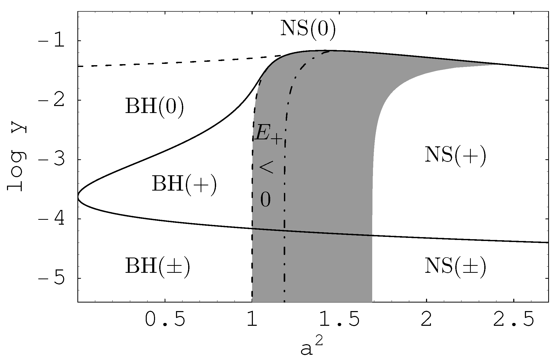
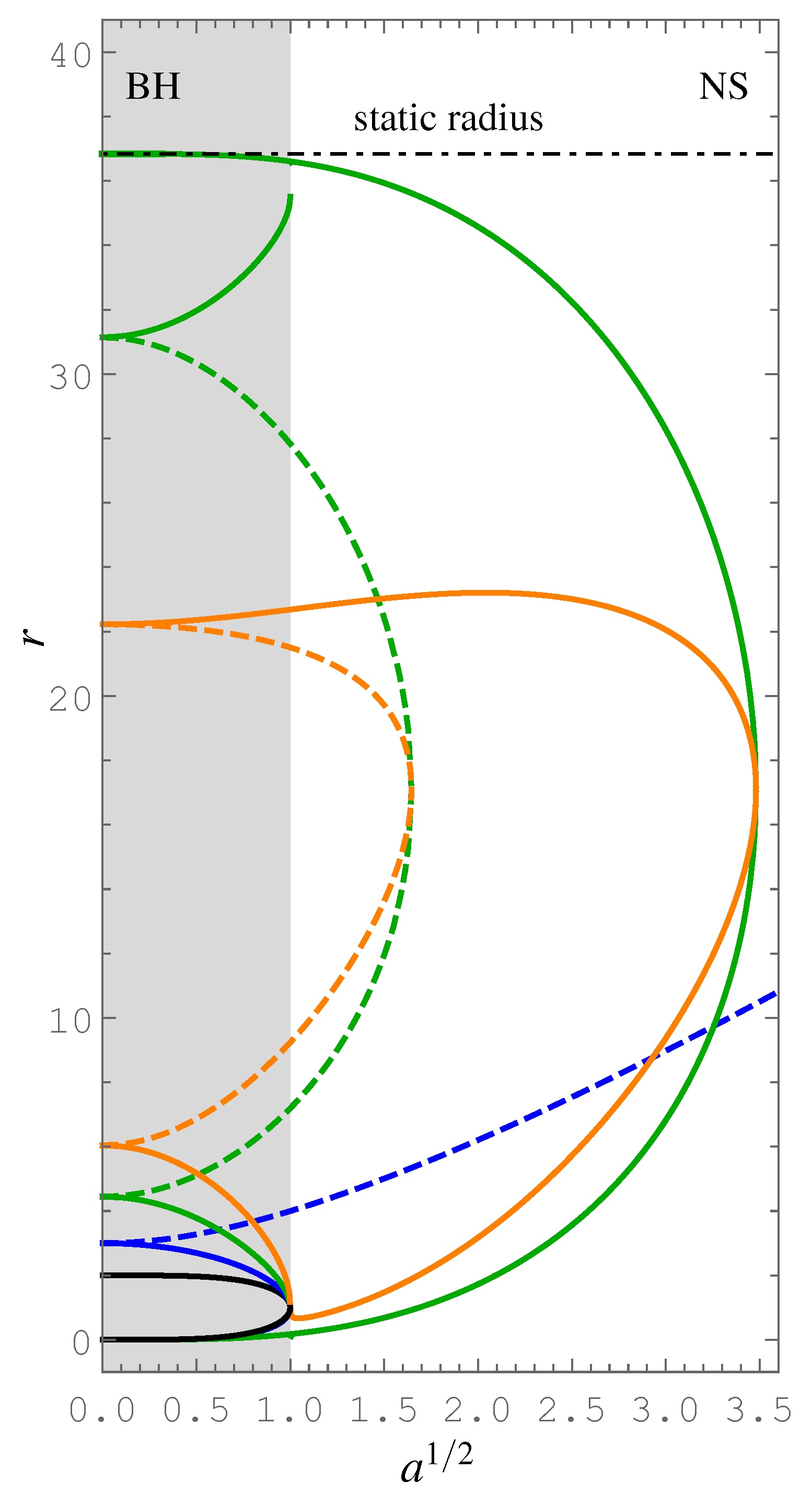
. No stable circular orbits exist for any value of the spin parameter a.
  • y crit ( ms + ) > y > y crit ( ms - ) . The function a ms ( 1 ) 2 ( r ; y ) ( a ms ( 2 ) 2 ( r ; y ) ) has a local maximum a ms ( max ) 2 (a local minimum a ms ( min ) 2 ) at the same radius r = r e ( ms ) . For a ms ( min ) 2 < a 2 < a ms ( max ) 2 , a 2 = a ms ( 1 , 2 ) 2 ( r ; y ) determines two marginally stable plus-family circular geodesics (an inner, and an outer one). For 0 < a 2 < a ms ( min ) 2 and a 2 > a ms ( max ) 2 , no stable circular geodesics exist.
  • y < y crit ( ms - ) . Two zero points of the function a ms ( 2 ) 2 ( r ; y ) correspond to its local minima, its local maximum a ms ( max 2 ) 2 occurs at r = r e ( ms ) , where the maximum of the function a ms ( 1 ) 2 ( r ; y ) is also located. For a 2 > a ms ( max ) 2 , no stable circular geodesics exist. For a ms ( max 2 ) 2 < a 2 < a ms ( max ) 2 , two marginally stable plus-family circular geodesics exist. For a 2 < a ms ( max 2 ) 2 , four marginally stable geodesics exist—the innermost and the outermost geodesics belong to the plus-family, the two orbits located in between belong to the minus-family; clearly, this last case corresponds to the black holes relevant in realistic astrophysical situations in the recent state of the Universe.
In Figure 4, the parameter space y- a 2 of the Kerr–de Sitter spacetimes is separated in accordance with the existence of stable circular geodesics, as determined by the functions a ms ( 1 , 2 ) 2 ( r ; y ) and y e ( ms ) ( r ) .
For fluid accretion tori, the notion of marginally bound circular geodesics is crucial, as it governs the innermost edge of accretion structures. In the Kerr spacetimes, these orbits are simply defined as unstable circular geodesics with specific energy E = 1 . The behavior of the effective potential (79) requires modification of the notion of the marginally bound orbits as unstable circular geodesics where a small radial perturbation causes infall of a particle from the orbit to the center or its escape to the cosmological horizon. Now, the two marginally bound orbits exist, as for some special value of the axial parameter L, denoted as L m b , the effective potential has two local maxima related by the condition
E ( + ) ( r mb ( i ) ; L mb , a , y ) = E ( + ) ( r mb ( o ) ; L mb , a , y ) ,
and corresponding to both the inner and outer marginally bound orbits as shown in Figure 4. The marginally bound orbits can be determined only by numerical methods; they can exist only in the KdS spacetimes admitting stable circular orbits—in the spacetimes with y 12 / 15 4 , the minus-family marginally bound geodesics thus do not exist. The positions of the photon, marginally stable and marginally bound circular orbits are given with dependence on the spin parameter a for a representative value of the cosmological parameter y in Figure 5; the behavior is qualitatively the same for all the black holes relevant in astrophysics.
The two marginally bound geodesics of given family determine the maximal extension of the fluid (pressure dominated) accretion structures in the Kerr–de Sitter black hole spacetimes; in a given Kerr–de Sitter black hole spacetime, the most extended corotating tori are wider than the counterrotating ones. For comparison, in Figure 4, we include the shape of the effective potentials defining both the inner and outer marginally stable geodesics of the plus family related to the special values of the specific angular momentum L ms ( i ) and L ms ( o ) . These two limiting effective potentials determine maximal possible extension of the Keplerian disks, as their inflexion points give the position of the inner and outer edges located at r ms ( i ) and r ms ( o ) . (Moreover, in given Kerr–de Sitter black hole spacetime, the corotating Keplerian disks can be more extended than the counterrotating ones). We thus clearly demonstrate that the Keplerian disks are more limited in both edges, in their extension in the Kerr–de Sitter black hole spacetimes, in comparison to the maximally extended thick fluid tori. Notice that the specific energy at the inner edge of the Keplerian disk is always smaller than the specific energy at the inner edge of any fluid torus, but the specific energy of the maximally extended Keplerian disk with r out = r ms ( o ) is slightly larger than the specific energy of the maximally extended fluid tori.
The efficiency of the Keplerian accretion process in the Kerr–de Sitter spacetimes is determined by the energy in the inner and outer edges of the Keplerian disk. While the inner edge is in the standard way defined as r in = r ms ( i ) , the outer edge can be defined in the range r ms ( i ) < r in < r ms ( o ) . The maximal efficiency of conversion of the rest mass into heat energy during accretion will be obtained in the limiting case of r out = r ms ( o ) , when it reads
η E ms ( o ) - E ms ( i ) ,
being thus limited from above by the specific energy of the outermost stable circular plus-family orbit, E m s ( o ) < 1 .
Note that the Kerr–de Sitter spacetimes can be for both black hole and naked singularity cases divided into three classes according to existence of stable circular geodesics, see Figure 1. For both plus and minus families, the stable orbits exist in the black hole class I, and naked singularity class V, only plus family stable orbits exist for black holes of class II and naked singularities of class VI, and no stable orbits exist for black holes of class III and naked singularities of class IV. The black holes of astrophysical relevance, related to the recently observed relic cosmological constant with y < 10 - 24 , belong to the class I; efficiency of the Keplerian accretion onto such black holes is in fact identical with those of the Kerr spacetime of the same spin a, although in principle it could be slightly decreased due the fact that for Kerr–de Sitter black holes there is E ms ( o ) < 1 . However, for larger values of y (much larger masses, or much larger values of the cosmological constant), the quantitative differences could be significant even for the class I black holes although the qualitative character remains kept. Much stronger differences can be related to the classes corresponding to the naked sigularity spacetimes. Detailed discussion of the efficiency of the Keplerian disks in the whole family of the Kerr–de Sitter spacetimes can be found in [13].

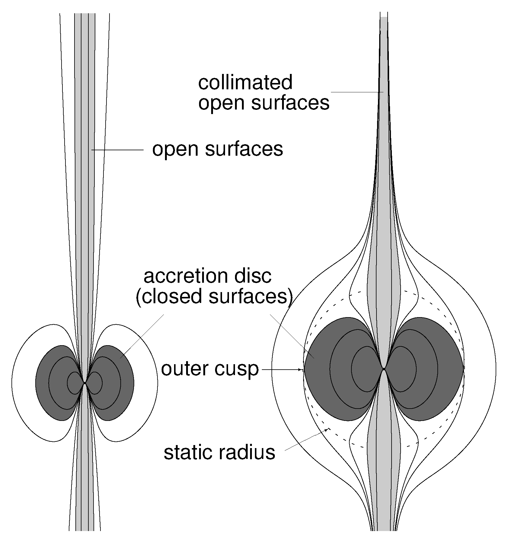
2.2. Toroidal Fluid Configurations and Collimation of Jets

The Keplerian accretion disks are usually related to accretion processes with low accretion rates, but, for high accretion rates, the pressure gradient will be relevant for the accretion configurations [3]. The simplest way of treating the fluid configurations is to assume the barotropic fluids where the pressure p is a simple function of energy density ϵ ) , enabling an elegant formulation of the theory of equilibrium configuration of this type.
Analytic theory of equilibrium configurations of rotating perfect fluid configurations was developed by Boyer [70]. The main result of the theory, the “Boyer’s condition”, states that the boundary of any stationary, barotropic, perfect fluid body has to be an equipotential surface. Here, we summarize application of the Boyer theory to the relativistic test perfect fluids orbiting in a stationary and axisymmetric way in the Kerr–de Sitter black hole spacetimes, as was introduced by Abramowicz and co-workers in the case of Schwarzschild and Kerr black holes [5,40], and used in the case of the Kerr–de Sitter spacetimes [14,71].

2.2.1. Pressure Equations and Effective Potential Governing Orbiting Perfect Fluid

Using the Euler equations governing stationary orbiting perfect fluid structures, we are able to determine both toroidal equilibrium and accretion structures when the equipotential surfaces are closed or cusped, and the limiting surfaces for non-equilibrium jets when the equipotential surfaces are open.
The stress-energy tensor of perfect fluid reads
T μ ν μ = ( ϵ + p ) U μ U ν + p δ ν μ ,
where ϵ and p are total energy density and pressure of the fluid, respectively. The test perfect fluid that is not influencing the spacetime structure is assumed to have the same symmetries as the Kerr–de Sitter spacetime, being stationary and axially symmetric and centered at the spacetime equatorial plane, similarly to the case of the Keplerian disks. Any orbiting element of the fluid has 4-velocity U μ = ( U t , 0 , 0 , U ϕ ) ; the orbital motion of the fluid is characterized by the vector fields of the angular velocity and the specific angular momentum of the fluid elements that are defined in terms of the 4-velocity field in the following way:
Ω = U ϕ U t , = - U ϕ U t .
These definitions imply the relation between the angular velocity Ω and the specific angular momentum governed by the spacetime geometry in the form
Ω = - g t t + g t ϕ g t ϕ + g ϕ ϕ .
The relativistic Euler equation governing the fluid motion follows from the projection of the conservation law μ T μ ν = 0 onto the hypersurface orthogonal to the 4-velocity U μ and in the axially symmetric configurations takes the form
i p ρ + p = - i ( ln U t ) + Ω i 1 - Ω ,
where i = r , θ . The specific energy of the fluid is determined by
( U t ) 2 = g t ϕ 2 - g t t g ϕ ϕ g t t 2 + 2 g t ϕ + g ϕ ϕ .
Furthermore, we can find the relation
U t U t = - 1 1 - Ω .
For a barotropic fluid determined by an equation of state given in the form p = p ( ϵ ) , the surfaces of constant pressure are determined according to the Boyer approach by the equipotential surfaces of the potential W ( r , θ ) defined as [40]
0 p d p ϵ + p = ln ( U t ) in - ln ( U t ) + in Ω d 1 - Ω W in - W ,
where the subscript “in” is referred to the inner edge of the torus. The points where i W = 0 correspond to the geodesic (free-particle) motion due to the vanishing of the pressure-gradient forces there.
The potential W = W ( r , θ ) given by Equation (70) can be determined if we specify the metric tensor of the spacetime and the “rotational law” of the fluid, i.e., the function Ω = Ω ( ) .
The simplest way to determine the rotation law is to assume the uniform distribution of the specific angular momentum in the torus
( r , θ ) = c o n s t ;
such a specification of the rotational law is important not only for its simplicity, but it also represents well all the fundamental properties of more complex physically relevant toroidal configurations. It is known that the tori with ( r , θ ) = c o n s t are marginally stable [72] and capable of producing maximal luminosity of all possible toroidal configurations [73]. The topological properties of the equipotential surfaces are shown to be rather independent of the distribution of the specific angular momentum ( r , θ ) , see [3,5,16,40,73]. For the fluid configurations with uniform distribution of the specific angular momentum, the potential is given by the simple formula
W ( r , θ ) = ln g t ϕ 2 - g t t g ϕ ϕ g t t 2 + 2 g t ϕ + g ϕ ϕ 1 / 2
being fully determined by the spacetime geometry.
In the Kerr–de Sitter spacetimes, the potential governing the barotropic fluid configurations is given by the formula
W ( r , θ ) = ln ρ 2 I 2 Δ r Δ θ sin 2 θ Δ θ ( r 2 + a 2 - a ) 2 sin 2 θ - Δ r ( - a sin 2 θ ) 2 1 / 2 .
The relevant properties of the equipotential surfaces are described by the behavior of the potential in the equatorial plane where it simplifies to the formula [5,14]
W ( r , θ = π / 2 ) = ln r 2 I 2 Δ r ( r 2 + a 2 - a ) 2 - Δ r ( - a ) 2 1 / 2 .
The reality conditions of the potential (74) read
Δ r 0 ,
( r 2 + a 2 - a ) 2 - Δ r ( - a ) 2 > 0 .
The first condition (75) simply means that the tori must be located at the stationary regions of the spacetime. Of course, we consider the stationary regions between the outer black-hole and the cosmological horizons. The second condition () is related to the photon motion, implying the inequality ph - < < ph + containing the effective potentials of the photon geodesic motion
ph ± ( r ; a , y ) = a + r 2 a ± Δ r ;
for an alternative definition of the effective potentials, see [67].
The local extrema of the function W ( r , θ = π / 2 ) are located at the radii where the given specific angular momentum coincides with the specific angular momentum of the Keplerian orbit, i.e., the circular geodesics that is given by [14]
= K ± ( r ; a , y ) ± ( r 2 + a 2 ) ( 1 - y r 3 ) 1 / 2 a r 1 / 2 [ 2 + r ( r 2 + a 2 ) y ] r 3 / 2 [ 1 - ( r 2 + a 2 ) y ] - 2 r 1 / 2 ± a ( 1 - y r 3 ) 1 / 2 .
These are the only local extrema of the potential W ( r , θ ) .
Now, we summarize properties of the fluid configurations in the Kerr–de Sitter black hole spacetimes, concentrating on the black holes of astrophysical relevance, allowing for existence of the stable circular geodesics of both the plus and minus families. Discussion of the properties of the equipotential surfaces of the orbiting fluid in the Kerr–de Sitter spacetimes of any class can be found in [14]; physical properties of such the tori were studied in [71]. The maximal extension of the toridal structures is determined by the positions of the marginally bound orbits related to these families; for nonzero spin, a > 0 , the corotating maximally extended tori are more extended than the counterrotating ones.
The equipotential surfaces are governed by the behavior of the Keplerian specific angular momentum K ± ( r ; a , y ) simultaneously with the photon potential ph ± ( r ; a , y ) as illustrated in Figure 6, where we chose spacetimes of the black hole class I admitting both the corotating and the counterrotating stable circular orbits. Behavior of the equipotential surfaces is demonstrated in Figure 7 by the meridional 2D sections. Closed equipotential surfaces govern equilibrium tori, while cusped (self-crossing) surfaces govern accretion tori allowing inflow of matter onto the black hole, or excretion tori allowing for outflow in direction to the cosmological horizon; both the inflow and outflow are governed by the so-called Paczynski mechanism of violation of the mechanical balance [5]. Open equipotential surfaces govern outflows in jets.
In the considered spacetimes, the Keplerian specific angular momentum radial profile K ( r ; a , y ) has for both families of circular geodesics two local extrema, ms ( i ) and ms ( o ) , corresponding to the inner and the outer marginally stable orbits. The local extreme of the photon potential determines the impact parameter of the circular null geodesic ph ( c ) . Two situations determined the behavior of the equipotential surfaces.
If the uniform distribution of the specific angular momentum is constant and ( ms ( i ) , ms ( o ) ) for the given family of orbits, the stationary toroidal configurations exist. For the corotating motion, the conditions
ms ( i ) + < < ph ( c ) + < ms ( o ) + or ms ( i ) + < < ms ( o ) + < ph ( c ) +
and, for the counterrotating motion, the conditions
ms ( i ) - > > ph ( c ) - > ms ( o ) - or ms ( i ) - > > ms ( o ) - > ph ( c ) -
imply that = c o n s t intersects K ( r ; a , y ) at three points corresponding to three geodesic orbits in the marginally stable configurations of the perfect fluid. The innermost and the outermost ones are unstable and determine the inner and the outer local maxima of the potential corresponding to the so-called “cusps” of the equipotential surfaces, respectively; the cusped equipotential surface govern accreting (inner unstable geodesic) or excreting (outer unstable geodesic) tori. The middle geodesic is stable and corresponds to the local minimum of the potential, i.e., the “centre” of the equilibrium (or accretion) configuration—see Figure 6 and Figure 7. Any physically relevant, stable distribution of the specific angular-momentum of the fluid configuration intersects the curve of the Keplerian angular momentum in three points corresponding to the possible existence of two cusps and one center in the fluid configurations governed by the equipotential surfaces.
In the second case, the = c o n s t tori satisfy the relations
ph ( c ) + < < ms ( o ) + or ph ( c ) - > > ms ( o ) -
implying that only two circular geodesics exist in the marginally stable configurations of the perfect fluid, corresponding to the center and the outer cusp of the configuration—the inner cusp and inflow of matter onto the black hole are forbidden.
The radial profile of the potential W given by (74) allows, for the parameter between ms ( i ) and ms ( o ) , the existence of two kinds of toroids—the one containing the inner cusp corresponding to accretion, the other containing the outer cusp where the accretion onto the central black hole is forbidden, but the outflows through the outer cusp are allowed, i.e., “excretion tori”. These two kinds of tori are separated by the specific angular momentum of the marginally bound circular geodesic, mb . For
ms ( i ) + < < mb + or ms ( i ) - > > mb - ,
the configurations correspond to the accretion tori, for
mb + < < ms ( o ) + or mb - > > ms ( o ) - ,
to the excretion tori. The case
= mb + or = mb -
corresponds to the marginally bound accretion tori (with largest extension) of a given family, see Figure 7. Colored regions correspond to the possible equilibrium toroidal configurations with a boundary given by any closed equipotential surface. Accretion (excretion) is possible through the inner (outer) cusp due to the violation of mechanical equilibrium when matter overfills the closed critical surface with the cusp (or cusps in the special case of = mb giving maximally extended tori)—the inner (outer) cusp naturally defines the inner (outer) edge of the accretion (excretion) toroids.

2.2.2. Limits on Extension of Toroidal Structures and Galaxy Extension

Surprisingly, the influence of the relic repulsive cosmological constant, or equivalently of a vacuum/dark energy, usually expected to be strong in the cosmological models, can be very important also in astrophysical situations related to the barotropic perfect fluid tori orbiting Kerr–de Sitter black holes. Physically relevant are the Kerr–de Sitter black holes allowing existence of stable circulargeodesics of the plus and minus families—these have the cosmological parameter in the range 0 < y < y crit 0.05924 . The crucial influence of the cosmological constant is given by the existence of outer edge of the toroidal configurations, limited by the static radius; there is no such restriction in the asymptotically flat Kerr spacetimes. However, it is relevant to have an estimate on the limits related to observable stellar mass, or supermassive black holes—then, we can obtain estimates of the cosmological parameter giving the related distance scales and express basic characteristics of the tori in astrophysical units.
The magnitude of the relic cosmological constant can be estimated, if we use the results of standard cosmological tests.2 Various cosmological observations indicate the present value of the vacuum energy density [74]
ϱ vac ( 0 ) 0.7 ϱ crit ( 0 ) ;
the present value of the critical energy density ϱ crit ( 0 ) is related to the Hubble parameter H 0 by
ϱ crit ( 0 ) = 3 H 0 2 8 π , H 0 = 100 h km s - 1 Mpc - 1 .
Using the estimated value of the dimensionless parameter h 0.7 , we obtain the “relic” repulsive cosmological constant
Λ 0 = 8 π ϱ vac ( 0 ) 1.3 × 10 - 56 cm - 2 .
Having this value of Λ 0 , we can determine the mass parameter of the spacetime, corresponding to any value of the cosmological parameter y, using the relation (). The most relevant are values of y corresponding to typical masses of black holes. For extreme black holes, we present in astrophysical units dimensions of the static radius and the outer marginally stable and marginally bound circular geodesics of both families (giving the limits on the extension of the Keplerian disks and toroidal configurations) in Table 1. The outer edge of tori is located between the outer marginally stable geodesic and the static radius, r ms ( o ) < r out < r s —the repulsive cosmological constant thus puts a natural limit on maximal extension of orbiting toroidal (test) structures in a given background. We can see that extension of the toroidal structures around stellar mass black holes is much smaller in comparison with extension of galaxies. However, different situation arises around supermassive black holes. For black hole masses M 10 6 M , the tori extension becomes comparable with extension of the central region of large galaxies. For very large supermassive black holes (with mass in the interval 10 8 M 10 10 M ), the dimensions of the test tori are roughly comparable with the dimensions of associated large galaxies [75]. We can thus conclude that the relic repulsive cosmological constant could represent a natural limit on extension of large galaxies [9], generally, on extension of the gravitationally bound systems immersed in Universe with expansion accelerated by the the relic cosmological constant [65]. These conclusions are strongly supported by the results related to polytropic configurations representing spherically symmetric galactic halos that have extension restricted by the static radius governed by the relic cosmological constant—calculations show that the mass and extension of galactic halos or halos of gravitationally bound galaxy clusters can be fitted by the polytropes constructed in spacetime with the relic cosmological constant [15]. Moreover, the internal parts of such polytropes could be gravitationally unstable to gravitational collapse forming black holes of mass M 10 9 M .
Note that the maximally extended tori related to the plus family geodesics are more extended than the maximally extended tori related to the minus family geodesics; see Figure 8.
The outer cusp of the toroidal structures plays another important role, as the matter outflow through the outer cusp (if large overfilling of the critical surface with the inner cusp when also the critical surface with the outer cusp is overfilled) could stabilize the torus against the dynamical instabilities, so-called run-away instabilities, as shown in [76].
There is a second crucial signature of the influence of the cosmic repulsion, connected with strong collimation of the open equipotential surfaces near the axis of rotation when compared with the Kerr case, supporting the collimation of the jets usually atributed to magnetic fields [77]; see Figure 9. This collimation becomes strong and clearly evident near and behind the static radius.3 The rotation of the background manifested by the dragging of inertial frames, see, e.g., [46,61], influences the shape of tori: the corotating tori are thicker and more extended than the counterrotating ones, generating narrower funnel where highly collimated relativistic streams of particles–jets are most probably created, see Figure 8.

3. Role of Magnetic Fields

The magnetic fields play a crucial role in the black hole physics [78]. The internal short-scale magnetic fields in the accretion disks orbiting black holes or neutron stars are assumed to be the source of viscosity causing the accretion, i.e., transfer of matter and angular momentum in the radial direction, due to the so-called magneto-rotational instability (MRI) [3,79]. Here, we concentrate on the large-scale external magnetic fields surrounding the Kerr black holes, and their influence on charged matter orbiting the black hole.
First, we discuss the role of the external magnetic fields in the charged test particle motion and its connections to the astrophysical processes, namely in the fate of ionized Keplerian disks and its possible relation to the high-frequency quasiperiodic oscillations (HF QPOs) observed in microquasars or some active galactic nuclei [22,31,32]. We emphasize the possible high importance of the Magnetic Penrose Process (MPP) [80] in the case of ionized Keplerian disks and related extreme acceleration of charged particles in the vicinity of the Kerr black hole horizon [10,33,39,81] influenced by radiation-reaction due to synchrotron radiation of escaping particles [36].4
Second, we discuss the influence of the external magnetic fields on the special charged toroidal structures levitating above (below) the black hole equatorial plane, complementary to the toroidal charged structures located in the equatorial plane. The tori are modeled as “dielectric” structures under assumption of zero conductivity, being thus complementary to the“force-free” structures constructed under assumption of infinite conductivity that are frequently used in the literature. The levitating charged structures could be, in dependence on the character of the external magnetic field, clouds located at the spacetime symmetry axis [19,82], or tori orbiting around the axis [18,83]. Clearly, in both cases, the off-equatorial charged non-conducting structures could potentially serve as the “lamp models” for irradiation of equatorial disks in the generation of profiled spectral lines [84].
The magnetic fields external to the black holes can be related to electric currents that could occur in the accretion disks [85], or to some external sources as the galactic magnetic fields, the magnetic field of the black hole companion, e.g., a magnetar [18], etc. In the vicinity of the supermassive black hole SgrA* in the Galaxy center, corresponding to few gravitational radii of the black hole, a highly ordered magnetic field of intensity ∼10–100 G is observed [86], around the central supermassive black hole at galaxy M87 the intensity of the magnetic field is ∼100 G [87], and recent study of variety of active galactic nuclei reported average intensity ∼10 4 G [88].
Let us stress that all the magnetic fields observed in the vicinity of astrophysical objects, including those observed near the surface of magnetars where B 10 15 G, can be considered as weak fields in the sense of general relativity, as their stress energy tensor is weak enough to enable abandoning of its influence on the spacetime structure [89]—the condition
B < < B G R = 10 18 10 M M G
is clearly satisfied for all the considered objects.

3.1. Magnetized Kerr Black Holes

The Kerr black hole spacetimes are governed by the line element that, in the standard Boyer–Lindquist coordinates ( t , r , θ , ϕ ) , and the system of geometric units ( G = 1 = c ), takes the form
d s 2 = g t t d t 2 + 2 g t ϕ d t d ϕ + g ϕ ϕ d ϕ 2 + g r r d r 2 + g θ θ d θ 2 ,
where
g t t = - ( 1 - 2 M r Σ ) ,
g t ϕ = - 2 a M r s i n 2 θ Σ ,
g ϕ ϕ = ( r 2 + a 2 + 2 a 2 M r Σ s i n 2 θ ) s i n 2 θ ,
g r r = Σ Δ ,
g θ θ = Σ ,
with
Δ = r 2 - 2 M r + a 2 , Σ = r 2 + a 2 c o s 2 θ ;
M is the gravitational mass of the black hole and a = J / M is its spin, J is its angular momentum. Assuming a > 0 , the Kerr black holes exist for a < M ; extreme Kerr black holes correspond to a = M , and Kerr naked singularities to a > M . The physical singularity has a ring character, being located at r = 0 , θ = π / 2 [52].
The Kerr metric (89) is asymptotically flat, i.e., far away from the black hole ( r ), the Kerr metric becomes Minkowski flat metric. In the following, we put again M = 1 , i.e., we use dimensionless spin a, dimensionless radial coordinate r, and dimensionless time coordinate t. For calculations of observationally relevant physical quantities, we introduce corresponding dimensional factors. The transformation to the Kerr–Schild coordinates is given in [52] and can be used for introduction of the Cartesian coordinates by the relations
x = r 2 + a 2 sin θ cos ϕ ˜ , y = r 2 + a 2 sin θ sin ϕ ˜ , z = r cos θ ,
where ϕ ˜ = ϕ - tan - 1 ( a / r ) .
There is no event horizon in the naked singularity spacetimes, in contrast to the Kerr black hole spacetimes (with a < 1 ) when two event horizons exist. In the Kerr geometry, two Killing vector fields exist, the stationary one, δ / δ t , and axial one, δ / δ ϕ that imply conserved energy E and axial angular momentum L of the particle motion.
We restrict our attention on the black hole spacetime region located above the event horizon at r + = 1 + ( 1 - a 2 ) 1 / 2 . The static observers can exist only in the regions where g t t < 0 . Above the event horizon, the static observers cannot exist in the ergosphere located under the so-called surface of stationarity, or stationary limit radius
r s t a t ( θ ) = 1 + ( 1 - a 2 cos 2 θ ) 1 / 2 .
In the Kerr geometry, it is convenient to introduce the locally non-rotating frames (LNRF) corresponding to the zero angular momentum observers (ZAMO) having axial angular momentum L = 0 , with four-velocity
u LNRF α = ( u LNRF t , 0 , 0 , u LNRF ϕ ) , ( u LNRF t ) 2 = g ϕ ϕ g t ϕ 2 - g t t g ϕ ϕ , u LNRF p h i = Ω LNRF u LNRF t ,
Ω LNRF ( r , θ ) = - g t ϕ g ϕ ϕ = 2 a r ( r 2 + a 2 ) 2 - a 2 Δ s i n 2 θ 2 .
The LNRFs 4-velocity is well defined at all r > r + , these frames are corotating with the Kerr spacetime at fixed coordinates r and θ . These ZAMOs can be considered as a generalization of the static observers in the Schwarzschild geometry—the particles falling from rest at infinity are purely radially falling relative to static observers in the Schwarzschild spacetimes, and relative to LNRFs in the Kerr spacetimes [90]; for the PNC (principal null congruence) photons, this property is in Kerr spacetimes realized in the so-called Carter frames, slightly modified against the LNRFs [60].

3.2. Asymptotically Uniform Magnetic Field as Basic Approximation

Clearly, the external magnetic field in the vicinity of the black hole horizon could be very complex, and the magnetohydrodynamical general relativistic dynamical simulations (MHGRD) of magnetized toroidal structures [1] indicate complex and highly dynamic magnetic fields in the tori, but the external magnetic field near the rotation axis of the structure, where the jets could be created, corresponds to a parabolic magnetic field independently from the initial form of the magnetic field. For this reason, it could be relevant to keep as the starting basic approximation the asymptotically uniform magnetic field introduced by Wald [23] and applied in many important studies of the astrophysical phenomena. In order to keep the symmetry of the spacetime configuration, it is necessary to assume that the magnetic field lines are directed along the spacetime rotation axis.5
The external, asymptotically uniform magnetic field of intensity B with lines oriented along the z-axis, i.e., orthogonal to the geometry equatorial plane, is governed by the electromagnetic 4-vector potential A α taking the form
A t = B 2 ( g t ϕ + 2 a g t t ) - Q 2 g t t - Q 2 , A ϕ = B 2 ( g ϕ ϕ + 2 a g t ϕ ) - Q 2 g t ϕ ,
where the induced electric charge of the black hole Q is also introduced. For non-charged black holes, there is Q = 0 , the maximal induced black hole charge generated by the black hole rotation takes the Wald value Q W = 2 a B (or Q W = 2 a B M if we keep the mass term)—see [23]. For the black holes having the maximal Wald charge, the electromagnetic potential reduces to the form
A t = B 2 g t ϕ - Q W 2 , A ϕ = B 2 g ϕ ϕ .
It is crucial that, even in this case, the A t component remains non-zero and can lead to a very strong acceleration mechanism for sufficiently massive black holes and strong magnetic fields. In the following, we restrict attention to the case with the maximal Wald induced charge Q W = 2 a B , as it represents the most relevant situations from the viewpoint of astrophysics. The four-potential of the magnetic field around the Kerr black hole then takes the form
A t = a B r Σ ( 1 + cos 2 θ ) - 1 ,
A ϕ = B 2 r 2 + a 2 - 2 M r a 2 Σ ( 1 + cos 2 θ ) .
Therefore, due to the dragging of frames and related twisting of magnetic lines, the black hole rotation generates a quadrupole electric field governed by the four-potential component A t . The corresponding “quadrupole” charge can be interpreted as an induced black hole charge [38,92]. The induction of the charge is canceled in the case of the extreme Kerr black holes when an analogy to the Meissner effect comes into the play—the black holes start to behave as a superconductor, expelling the magnetic field lines [93].
We can say generally that, if the magnetic field has a non-zero poloidal component, then any observer located in the ergosphere can detect a non-zero electric field [23,94]. Of course, the induced electric charge giving the electrostatic energy for particle acceleration should not be screened by plasma [95]—as shown in [96], the total screening needs the conditions
B . E = 0 , E 2 - B 2 < 0
to be satisfied simultaneously, where E and B are vectors of the electric and magnetic field as measured in the LNRFs. It can be shown [96] that E 2 - B 2 is negative outside the ergosphere, but it is positive inside the ergosphere. Therefore, inside the ergosphere, the induced electric field generated by combined effect of uniform (generally poloidal) magnetic field and the black hole rotation is not screened and can serve for efficient acceleration—it increases with increasing magnetic field intensity and increasing black hole spin, as follows from Equation (99). It has been shown recently that, in the case of the SgrA* supermassive black hole, the electric charge related to the gravitationally induced electric field cannot overcome 10 15 C—this is at least five orders smaller than the electric charge related to extremal charged black holes, guaranteeing thus that its influence on the black hole spacetime structure is negligible [92].
The magnetic fields weak from the point of view of their influence on the spacetime structure can be very strong from the point of view of their influence on the motion of charged matter. Let us consider a charged matter treated as a test particle with charge q and mass m being under influence of a black hole with mass M, immersed in an external asymptotically uniform magnetic field of the strength B. The interplay of the electromagnetic Lorentz force and the gravity acting on the charged matter, represented by the specific charge q / m , can be reflected by a dimensionless “magnetic parameter” B introduced in [20,32]
B = B 2 q m G M c 4 .
With dependence on the black hole mass parameter M, we can consider as “charged test particles" electrons, protons, ions, massive charged inhomogeneities as charged dust or plasma objects similar to “ball lightnings”, orbiting in the innermost region of the accretion disk or in its vicinity, or even neutron stars and stellar black holes orbiting in the vicinity of a supermassive black hole—the specific charge q / m of such objects ranges from the electron maximum to zero. For protons and ions, and especially for electrons, the magnetic parameter B can be very large even for relatively weak magnetic fields due to the large magnitude of their specific charge q / m , implying thus strong influence of the electromagnetic Lorentz force on their motion even in weak magnetic fields. For example, around a stellar mass black hole having M 10 M , we have the magnetic parameter of magnitude B = 0 . 004 both for an electron moving in the magnetic field B 10 - 5 G , or a charged dust grain (one electron lost, m = 2 × 10 - 16 kg) moving in the magnetic field B 10 9 G —the character of the test particle motion is the same in both cases. In Table 2, we present a similar comparison including protons and ions.
There are two relatively simple alternatives to the basic approximation of the external magnetic field by its uniform form. The first alternative to the uniform field approximation of the external magnetic field is represented by widely discussed dipole magnetic field generated by a circular current loop in the central plane of the Schwarzschild geometry at the radius a 2 . At the outer region of this solution, at r > a , the four-vector electromagnetic potential A μ in the Schwarzschild metric is given by the nonzero covariant component taking the form [85]
A ϕ D = B 2 ln 1 - 2 M r + 2 M r 1 + M r g ϕ ϕ .
Note that the second term in square brackets is negative for r > 2 .
The second possibility of alternative simple approximation is represented by phenomenological parabolic magnetic fields indicated by predictions of computational simulations-magneto- hydrodynamic fluid models of thick accretion disks orbiting a black hole demonstrate final creation of a parabolic magnetic field in the vicinity of the black hole rotation axis, independently of the original configuration of the external magnetic field entering the orbiting matter [97]. The parabolic magnetic field is determined by the four-vector electromagnetic potential taking the form [97]
A ϕ P = B 2 r k ( 1 - | cos ( θ ) | ) ,
where the parameter k represents declination of the field lines relative to the rotation axis.
Our studies related to ionized Keplerian disks orbiting magnetized Schwarzschild black holes demonstrated that the consequences of the ionization are qualitatively the same in all three alternative approximations of the external magnetic field, even for disks located originally under various inclination angles to the magnetic field lines [10]. Therefore, in order to obtain the basic ideas and intuition on the role of the external magnetic fields, the uniform magnetic field basic approximation that can be treated in the simplest way in mathematical modeling could be quite sufficient.
The Keplerian disk has to bee composed of matter that behaves as electrically neutral in the presence of the electromagnetic field. This condition can be satisfied for a plasmatic disk composed from quasi-neutral soup of electrons and protons (ions), if its density is high enough, implying that the main free path of the charged particles is substantially shorter than the orbit around the black hole. The charged particles circulate around the black hole collectively as an electrically neutral matter and influence of the electromagnetic field is irrelevant. At the edge of the disk, the density decreases and the electromagnetic field enters the play as the mean free path increases, being comparable with extension of the orbital motion.
The astrophysical relevance of the properties of the charged particle motion in the combined gravitational and electromagnetic field has a limit that strongly depends on the intensity of the electromagnetic interaction. The limits on validity of the test particle motion arise due to possible strong influence of the radiation of the charged particles. We discuss the back-reaction of the radiation of charged particles on their motion i detail later.

3.3. Motion of Charged Test Particles

Motion of a charged test particle is governed by the Lorentz equation
m D u μ D τ = e F ν μ u ν ,
where τ is the proper time of the moving particle. The Lorentz equations represent four second order differential equations; however, we could make substantial simplifications due to the symmetries of the background. Contrary to the case of the Kerr–Newman black holes where the Lorentz equations can be separated and given in terms of first integral governing fully regular test particle motion [52,64]; in the case of magnetized Kerr black holes, the motion has generally chaotic character.

3.3.1. Hamiltonian Formalism and Effective Potential of the Motion

Due to the symmetries of the background, corresponding to the magnetized Kerr black holes with the uniform magnetic field lines orthogonal to the equatorial plane of the spacetime geometry, it is convenient to use for the solution of the motion equations the Hamiltonian formalism. The Hamiltonian can be written in the form
H = 1 2 g α β ( π α - q A α ) ( π β - q A β ) + 1 2 m 2 ,
where the generalized (canonical) four-momentum π μ = p μ + q A μ is related to the kinematic four-momentum p μ = m u μ and the influence of the electromagnetic field q A μ . The equations of motion are then reduced to the Hamilton equations
d x μ d ζ p μ = H π μ , d π μ d ζ = - H x μ
and the affine parameter is related to the particle proper time due to relation ζ = τ / m . The Hamilton equations represent generally eight first order differential equations enabling precise numerical integration by the symplectic integrator method [98].
The combined gravitational and electromagnetic background of the magnetized Kerr black holes as considered here is stationary and axially symmetric allowing thus for reduction of the charged test particle motion to a two-dimensional dynamics—we can introduce two constants of the motion: energy E and angular momentum L given by the conserved components of the canonical momentum
- E = π t = g t t p t + g t ϕ p ϕ + q A t , L = π ϕ = g ϕ ϕ p ϕ + g ϕ t p t + q A ϕ .
For further discussion, it is convenient to introduce the specific energy E = E / m , the specific axial angular momentum L = L / m , and the magnetic interaction parameter B = q B / 2 m . We thus obtain Hamiltonian with two degrees of freedom, and 4D phase space ( r , θ ; p r , p θ ) that can be expressed in the form
H = 1 2 g r r p r 2 + 1 2 g θ θ p θ 2 + H P ˜ ( r , θ ) ,
enabling introduction of the effective potential of the radial and latitudinal motion giving the energetic boundary for the particle motion ( H P ˜ = 0 ). The energy condition relates the specific energy to the effective potential due to the equation
E = V eff ( r , θ ) ,
where
V eff ( r , θ ) = - β + β 2 - 4 α γ 2 α ,
with
β = 2 [ g t ϕ ( L - q ˜ A ϕ ) - g t t q ˜ A t ] , α = - g t t , γ = - g ϕ ϕ ( L - q ˜ A ϕ ) 2 - g t t q ˜ 2 A t 2 + 2 g t ϕ q ˜ A t ( L - q ˜ A ϕ ) - 1 .
The effective potential defined here is properly chosen for the region above the outer horizon of the black hole; for subtleties related to the inner region of the Kerr geometry, see, e.g., [99]. Above the outer (event) horizon, the effective potential governs the regions allowed for the motion of a charged particle with fixed value of the axial angular momentum.

3.3.2. Circular Orbits of Charged Test Particles

Around magnetized black holes, the charged particle motion is generally chaotic. However, the circular motion in the equatorial plane, and the associated epicyclic motion in the equatorial plane and its vicinity represent an exception [31,32]. The circular orbits are very important from the astrophysical point of view as they govern the thin (Keplerian) accretion disks, and even the toroidal fluid configurations.
The circular orbits of charged test particles are determined by the local extrema of the effective potential, governed by the relations V eff r = 0 and V eff θ = 0 . As equation V eff θ = 0 holds generally at θ = π / 2 , equatorial circular orbits exist and were widely discussed in [31,32], but existence of the off-equatorial circular orbits has been also demonstrated in [17]. Here, we focus attention on the equatorial circular orbits.
In [32], it has been demonstrated that the circular orbits can be separated into four classes:
Prograde anti-Larmor orbits (PALO) where the particle is corotating ( L > 0 ), magnetic lines are co-oriented with the black hole rotation axis, B > 0 , Lorentz force is repulsive;
Retrograde Larmor orbits (RLO) with the particle counter-rotating ( L < 0 ), magnetic lines co-oriented with the black hole rotation axis ( B > 0 ), Lorentz force attractive;
Prograde Larmor orbits (PLO) with L > 0 , magnetic field lines oriented inversely to the black hole rotation axis, B < 0 , Lorentz force attractive;
Retrograde anti-Larmor orbits with L < 0 , magnetic field lines oriented inversely to the black hole rotation axis B < 0 , Lorentz force repulsive.
In the case of magnetized non-rotating Schwarzschild black holes, classes PALO/RALO, and RLO/PLO coincide.
The circular motion is stable relative to radial (vertical) perturbations, if 2 V eff r 2 > 0 ( 2 V eff θ 2 > 0 ). In the opposite cases, the motion is unstable against radial (vertical) perturbations. The vanishing of the second derivative of the effective potential corresponds to the innermost (marginally) stable circular orbit representing the inner edge of the Keplerian disks [4].
Detailed analysis of the charged particle circular orbits in the background of Kerr black holes immersed in an asymptotically uniform magnetic field with lines orthogonal to the geometry equatorial plane can be found in [32]. In the case of magnetized Schwarzschild black holes, the charged particle circular orbits were treated in [31,35]; for dipole and parabolic magnetic fields around a Schwarzschild black hole, the circular orbits were discussed and similarity to the case of the uniform magnetic fields was demonstrated in [10].

3.4. Ionized Keplerian Discs around Magnetized Black Holes

Discussing the fate of ionized Keplerian disks orbiting magnetized black holes, we have to distinguish the case of non-rotating black holes when the Keplerian disk can be located in any of the central planes of the Schwarzschild geometry, and the case of rotating black holes when the Keplerian disk has to be located in the equatorial plane of the Kerr geometry, or its vicinity, due to the Bardeen–Peterson effect forcing any inclined disk to be located in the Kerr geometry symmetry plane due to the combined effect of the disk viscosity and the frame dragging of the Kerr spacetime [2].
The study of the dependence of the fate of a Keplerian disk orbiting a Schwarzschild black hole on the inclination angle of the disk to the magnetic field lines of the uniform magnetic field was presented in [35]; the results obtained for the magnetic fields of the dipole and the parabolic type were presented in [10] where it has been explicitly demonstrated that the fate of the Keplerian disk is qualitatively the same for all three considered cases (uniform, dipole, parabolic) of the external magnetic field. Therefore, being inspired by these results obtained for the Schwarzschild spacetimes [10], we consider here as sufficiently representative the case of the uniform magnetic fields with lines parallel to the Kerr geometry axis, using the fact that it is the simplest case for mathematical modeling, being in addition highly illustrative for basic ideas behind the fate of Keplerian disks.
We assume that matter of the Keplerian disk following circular geodesics of the spacetime becomes ionized in the internal disk region near the innermost circular geodesics due to irradiation or some other ionization mechanisms, starting to feel the influence of the electromagnetic field (see [33]). In order to determine the fate of the disk, i.e., motion of the charged particles of the ionized disk, the method of the effective potential seems to be most efficient [22,32,33]. Position of the circular charged particle orbits in the combined gravo-electromagnetic field is determined by the local minima of the effective potential corresponding to their canonical axial angular momentum—the crucial role is played by the innermost stable circular orbit (ISCO) representing standard limit on stable circular motion [32]; no circular (or bound) motion is allowed for particles with the canonical axial angular momentum smaller than those corresponding to the marginally stable circular orbit L ms [32].
If the canonical (conservative) axial angular momentum of the ionized particle L is large enough to allow for existence of a stable circular orbit, the effective potential has minimum determining the energy of the particle following the circular orbit E ms . The fate of the charged particle then depends on its canonical (conservative) energy E > E ms , and is determined by the shape of the effective potential at the given energy level, E = V eff ( r , a , L ) .

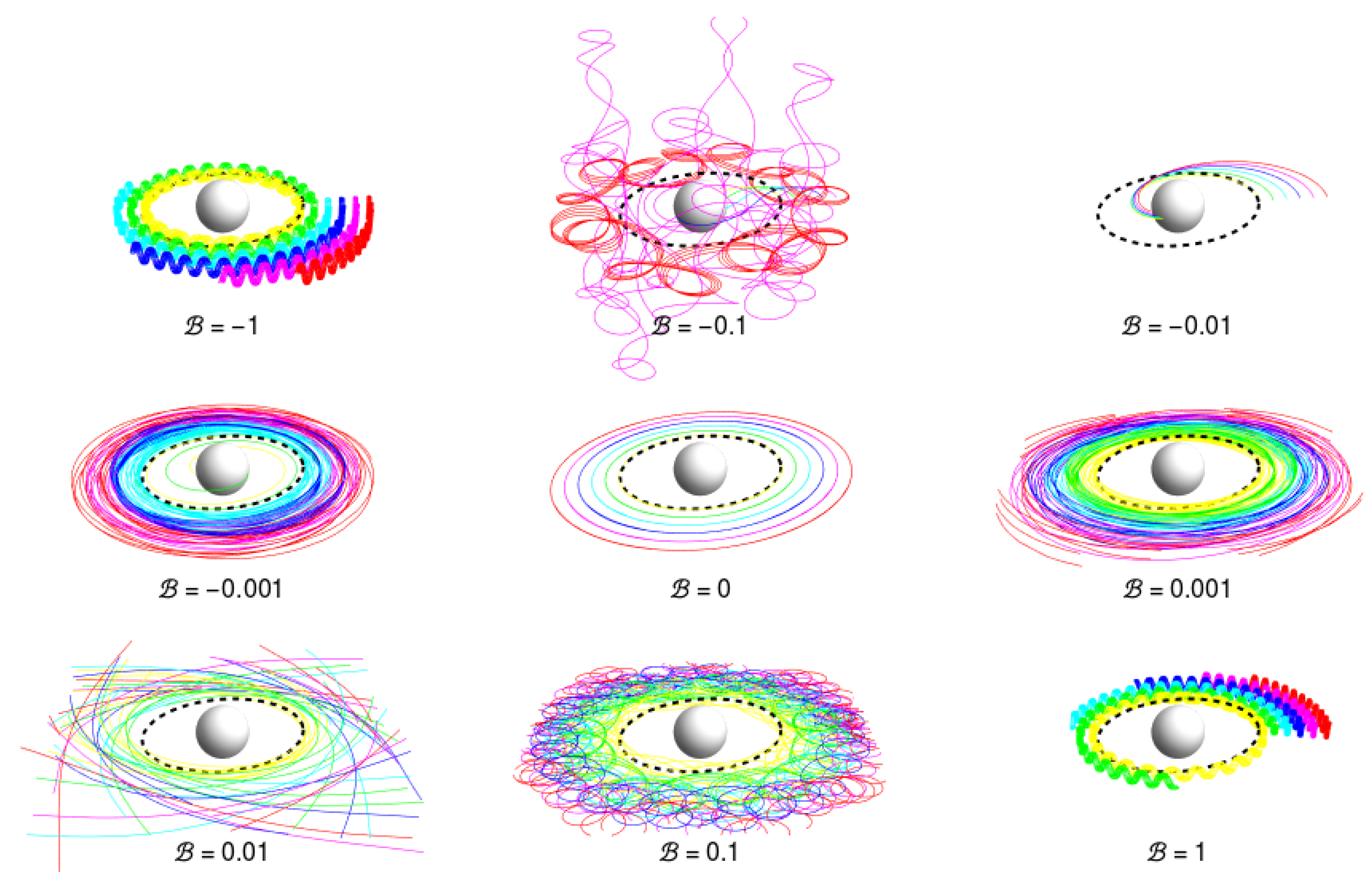
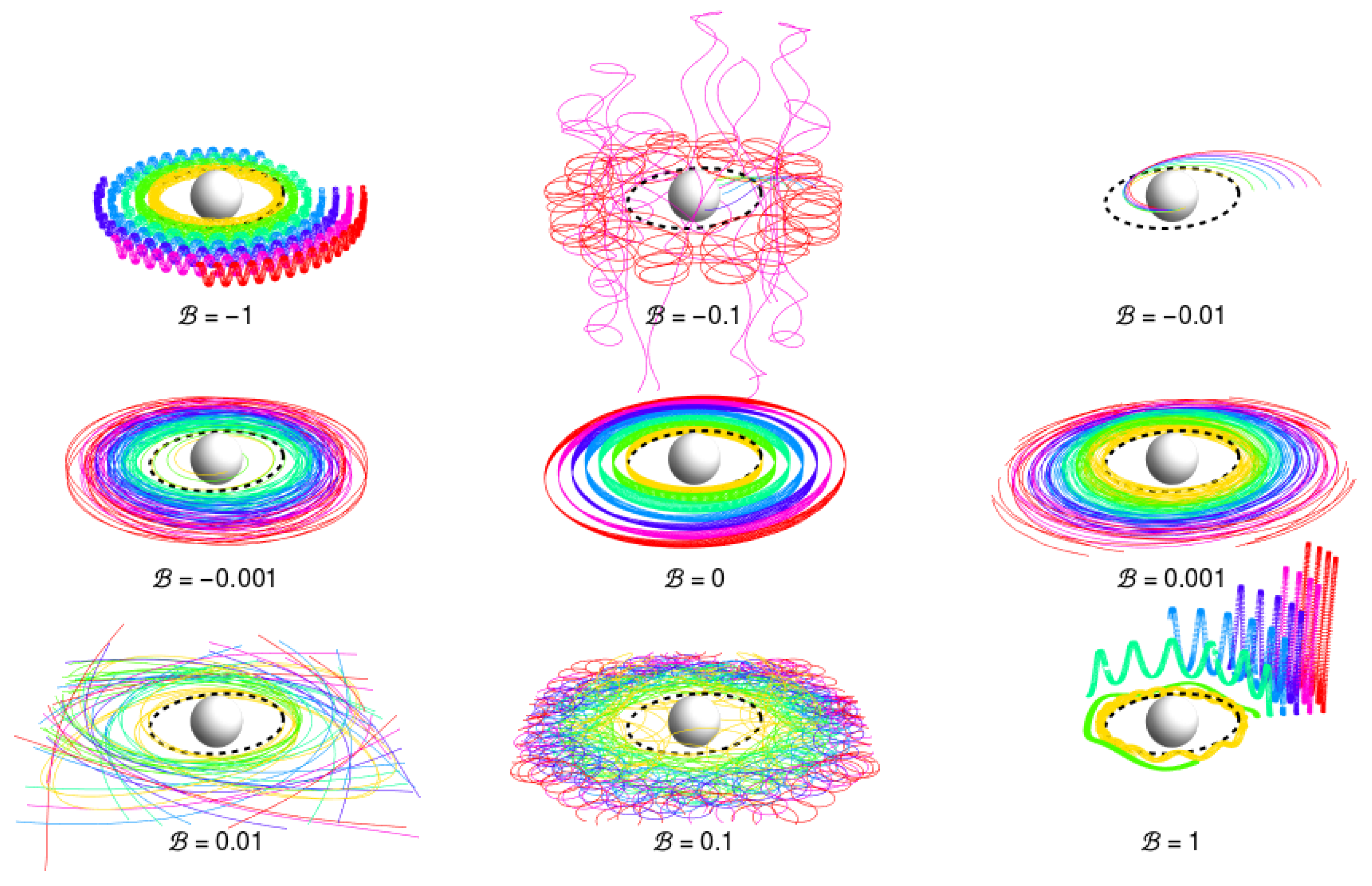
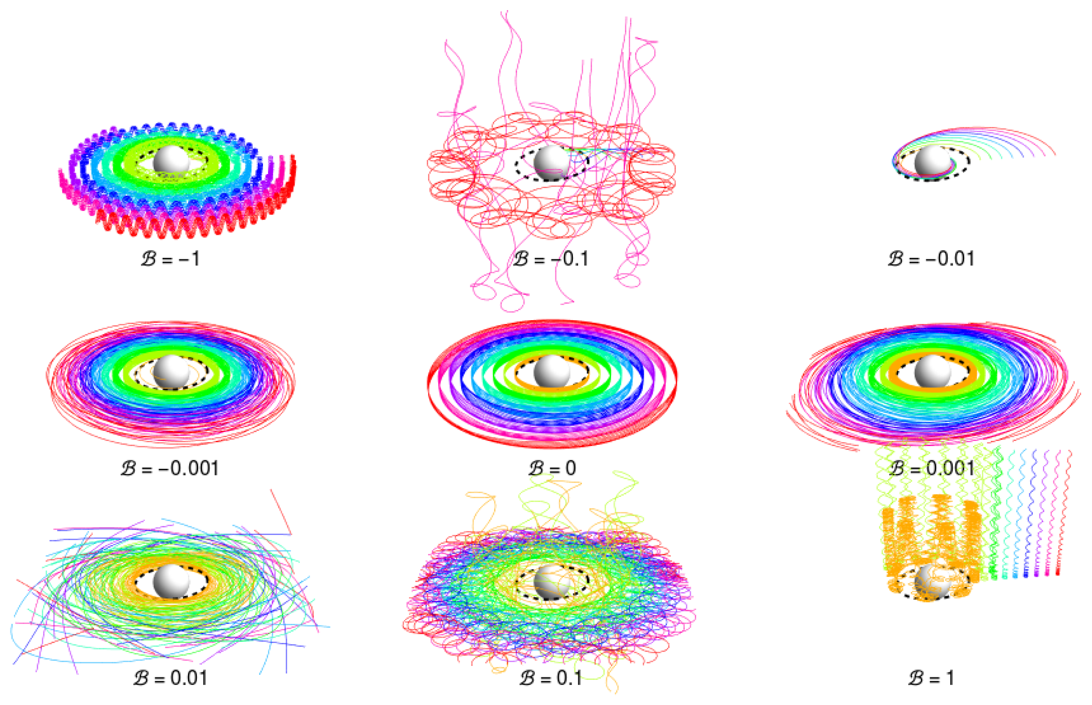
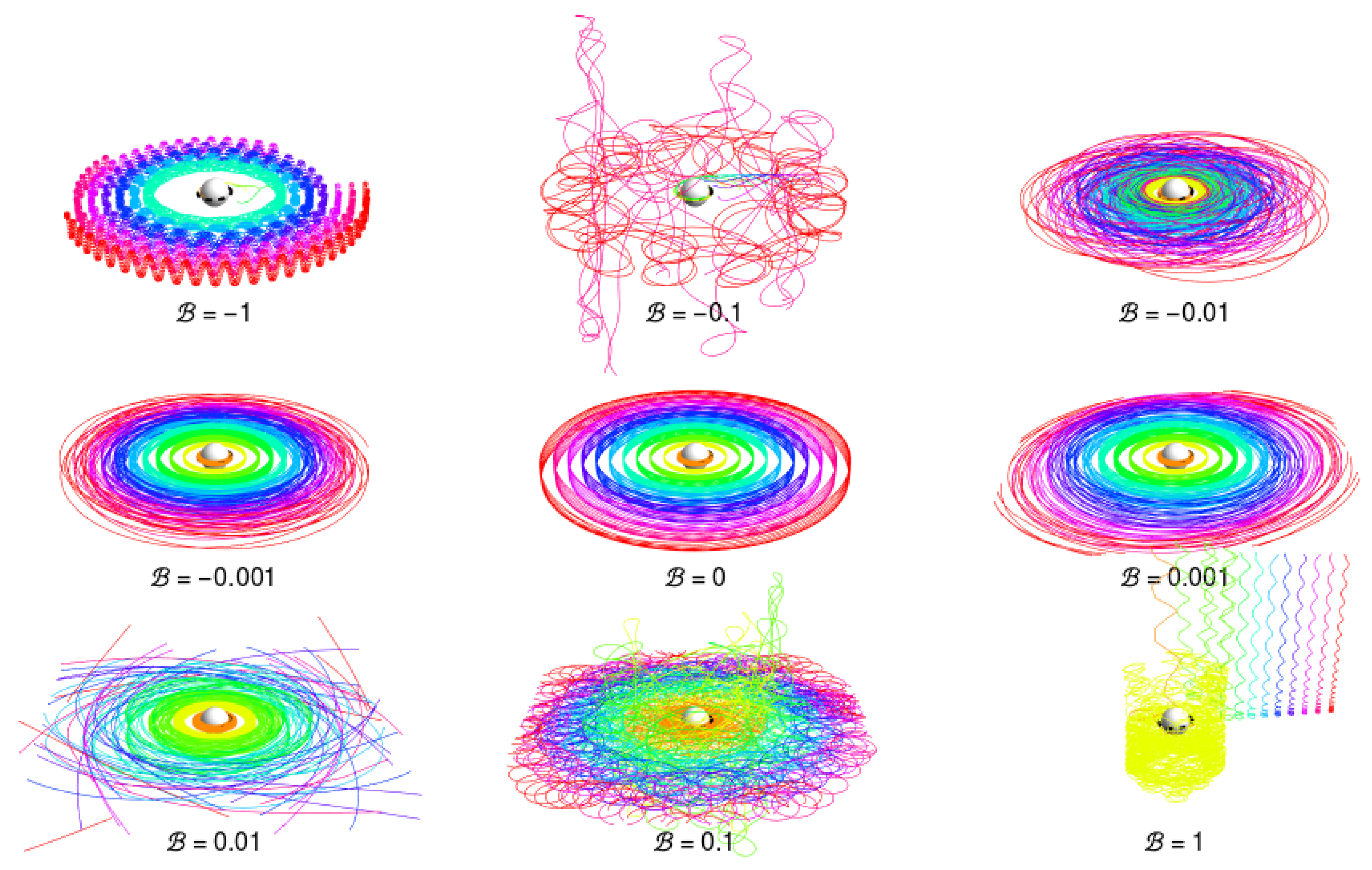
3.4.1. Possible Fates of Ionized Keplerian Disks

The ionized Keplerian disks were studied in detail for the magnetized non-rotating black holes [31,35]. For magnetized rotating black holes, the ionized Keplerian disk were partially studied in [22,32,33,34]. Here, we present all the variants of the fate of the ionized Keplerian discs orbiting a magnetized Kerr black hole, demonstrating existence of four regimes of the developments of ionized Keplerian discs:
(a) Survival of the Keplerian disk in regular oscillatory epicyclic motion around circular orbits that could be related to the twin high-frequency quasiperiodic oscillations (HF QPOs) observed in the X-ray spectra of some microquasars.
(b) Transformation of the Keplerian disk into a geometrically thick toroidal accretion structure due to fully chaotic motion of ionized particles.
(c) Destruction of the Keplerian disk due to direct infall of ionized matter into the black hole.
(d) Destruction of the Keplerian disk due to chaotic scattering of charged particles causing their escape along the magnetic field lines to infinity; in this case, ultra-high energy particles can be generated due to the MPP, if the Lorentz force is large enough.
The case of the effective potential section open to the black hole horizon (case b) corresponds clearly to the destruction of the Keplerian disk by direct infall, while the section open to infinity (case c) governs destruction of the disk by escape to infinity. On the other hand, the closed section corresponding to bound orbits (case a) governs the regular epicyclic motion, if the charge particle energy is low enough that the approximation of linear harmonic oscillations can be relevant, or chaotic motion, if the energy is high enough. The second case of the chaotic motion can be for very high energies shifted to the process of chaotic scattering [33] causing transformation from the circular regular motion to a final state of regular motion along the magnetic field lines demonstrating potentially an extremely efficient version of the MPP [39]. We briefly expose both the epicyclic motion, and the chaotic scattering.

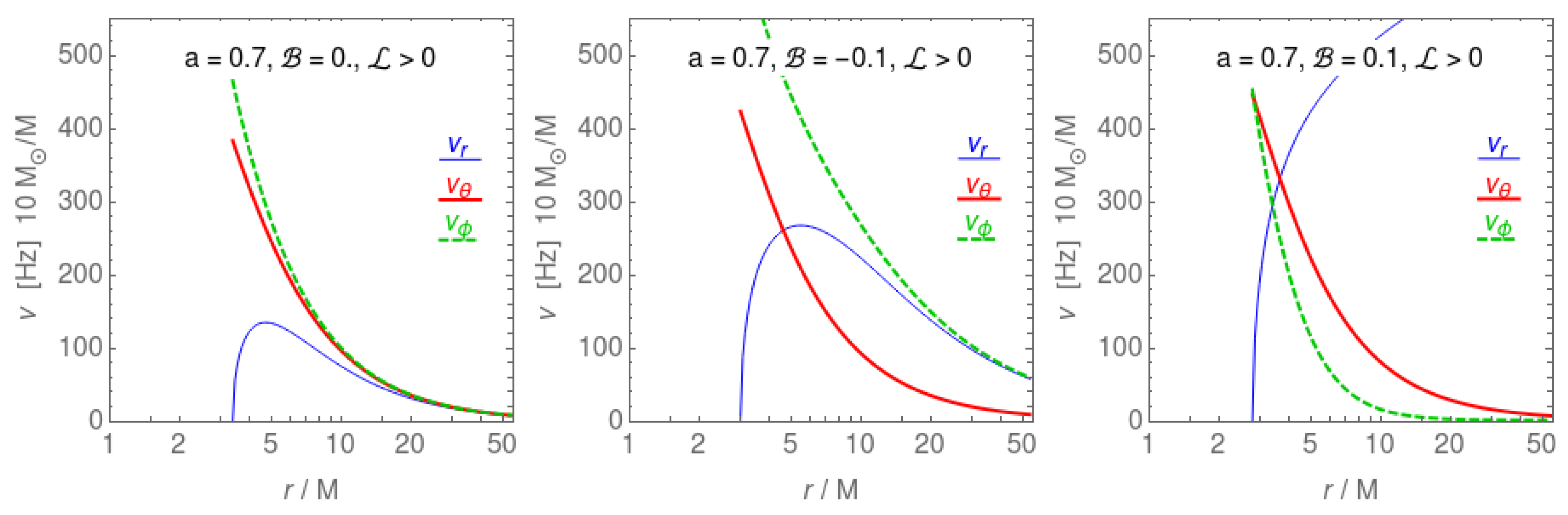
3.4.2. Regular Epicyclic Motion and Explanation of HF QPOs in Microquasars by Magnetically Modified Geodesic Models

Although the motion of charged particles around magnetized black holes is generally chaotic, according to the Kolmogorov–Moser–Arnold theorem in the vicinity of the minima of the effective potential, i.e., for energies sufficiently close to the energy of stable circular orbit with given axial angular momentum, the charged particle can follow an epicyclic motion in radial and vertical directions, governed by the equations of fully regular linear harmonic motion [32]. The frequencies of the harmonic oscillatory motion around a stable circular orbits are governed by the second derivatives of the effective potential at the position of the static circular orbit, as shown in [31,32].6 Here, we demonstrate an alternative approach to determine the epicyclic frequencies, based on direct application of the equations of motion and their perturbations [22].
The four-velocity of the circular orbits has two non-zero components, u μ = ( u t , 0 , 0 , u ϕ ) . For the maximally charged magnetized Kerr black holes (with Q W ), the Lorentz equation implies the radial component of the equatorial motion in the form
( a 2 - r 3 ) ( u ϕ ) 2 - 2 B ( r 3 - a 2 ) u ϕ - 2 a ( u ϕ + B ) u t + ( u t ) 2 = 0 ,
while the normalization condition for the four-velocity gives
( a 2 ( 2 + r ) + r 3 ) ( u ϕ ) 2 - 4 a u ϕ u t - ( r - 2 ) ( u t ) 2 + r = 0 .
Determination of a circular orbit at a given radius r by the four-velocity components u t and u ϕ is an alternative to determination by the motion constants L and E . The orbital frequency at the circular orbit Ω ϕ , related to distant observers and called also Keplerian frequency, Ω K , and the Larmor frequency, related purely to the external magnetic field, Ω L , are determined by the relations:
Ω ϕ Ω K = d ϕ d t = u ϕ u t , Ω L = q B m u t = 2 B u t .
The epicyclic motion of a charged particle, given by the world-line x μ ( τ ) and concentrated around the “equilibrium” stable circular orbit with x 0 μ ( τ ) governed by the canonical axial angular momentum of the charged particle, is determined by deviation vector ξ μ ( τ ) = x μ ( τ ) - x 0 μ ( τ ) . Introducing the deviation vector into the Lorentz equation, we arrive in the first order expansion at small deviations to the equations of linear harmonic oscillations in the vertical and radial directions [25]
d 2 ξ l d t 2 + Ω l 2 ξ l = 0 , l = θ , r ,
where Ω θ ( Ω r ) is the angular frequency of the particle vertical (latitudinal) or radial epicyclic motion related to the coordinate time t, i.e., measured by distant static observers. For the maximally charged magnetized Kerr black holes with the maximal Wald charge Q W , we arrive to the relations [22]
Ω r 2 = γ u ϕ ( u ϕ + 2 B ) + ν u t ( u ϕ + B ) + ρ ( u t ) 2 + σ r 5 ( u t ) 2 ,
and
Ω θ 2 = α u ϕ ( u ϕ + 2 B ) + β u t ( u ϕ + B ) + 2 a 2 ( u t ) 2 r 5 ( u t ) 2 ,
where
α = r 5 + a 2 r 2 ( 4 + r ) + 2 a 4 , β = - 4 a ( r 2 + a 2 ) , γ = r 4 ( - 8 + 3 r ) + a 2 r ( 2 - 10 r + r 2 ) - 4 a 4 , ν = 4 a ( 2 a 2 - r + 3 r 2 ) , ρ = 2 ( - 2 a 2 + r - r 2 ) , σ = 4 B 2 r ( ( - 2 + r ) r 3 - a 2 ( 1 + 2 r ) ) .
The frequencies determining the orbital and epicyclic motion of charged particles represent generalization of the frequencies related to the epicyclic geodesic motion. As the frequencies are given in dimensionless form, we have to use the formula
ν i = c 3 2 π G M Ω i [ H z ] ,
where i = ( ϕ , r , θ ) , if we are interested in directly observable frequencies given in physical units.
The radial profiles of the orbital and epicyclic frequencies of the charged particle motion in the field of magnetized black holes have several properties fundamentally different in comparison with the radial profiles of the frequencies characterizing the geodesic epicyclic motion—however, the crucial effect of vanishing of the radial epicyclic frequency ν r at the marginally stable circular orbit holds in both cases [22]. The “magnetically induced” modifications of the radial profiles of the orbital and epicyclic frequencies of the charged particle motion enable more efficient application of the magnetically modified geodesic models of the the twin HF QPOs observed in some microquasars [102] or active galactic nuclei [103].7 We thus present a short overview of the special properties of the radial profiles of the “magnetized” orbital and epicyclic frequencies. The properties are related to the four families of the circular orbits of charged particles orbiting a magnetized Kerr black hole as introduced in [32].
The most important differences between the radial profiles of the orbital and epicyclic frequencies in the magnetized and purely geodesic cases occur for the frequencies ν r and ν ϕ = ν K —due to the strong effect of the Lorentz force in the radial direction. The Lorentz force increases the radial epicyclic frequency ν r , namely for the PALO and RALO orbits, but the axial (Keplerian) frequency ν K decreases for such orbits. Inversely, the radial profile of the latitudinal (vertical) epicyclic frequency ν θ cannot be significantly influenced by the magnetic field because of the direction of the Lorentz force. The other crucial difference corresponds to the relation of the magnitudes of the three considered frequencies—for the geodesic motion the relation ν r < ν θ < ν ϕ holds at all radii of the radial profiles around non-extreme black holes8, for the magnetized orbits, the interrelations between the three frequency radial profiles strongly depend on the type of the orbit. Nevertheless, the difference most relevant from the point of view of astrophysics occurs for all four types of the circular orbits—the point of intersection of the ν r and the ν θ profiles occurs above the ISCO radius. For the PALO and RALO orbits, there is intersection of the ν ϕ and the ν r radial profiles, and for the PALO orbits even the crossing of the ν θ and the ν ϕ radial profiles can occur.
The crossings of the orbital and epicyclic frequency radial profiles have important astrophysical consequences that could lead to significant observable signatures as vanishing of the nodal shift of orbiting matter. In the case of the RALO orbits, we observe possibility that at some radii the orbital frequency is much smaller than both the epicyclic frequencies, ν ϕ < < ν r ν θ enabling the toroidal type of the charged particle motion required in the kinetic model [106]. In Figure 10, we present typical types of the radial profiles of the “magnetized” frequencies—notice that the magnetized frequency radial profiles are similar to radial profiles of the frequencies of the string loop oscillations [100,101].
The so-called geodesic models proposed to explain the twin HF QPOs observed in microquasars, i.e., binary systems composed of a black hole and a companion star, use the frequencies of the orbital and epicyclic geodesic motion—-for detailed overview, see [104]. The twin HF QPOs are two peaks of the X-ray power density observed in the case of microquasars in the frequency range ν 100 –400 Hz; we can thus assume their creation in the innermost parts of the Keplerian accretion disks as the observed frequencies are close to the frequency of the orbital Keplerian motion near the ISCO of the stellar mass black holes with mass in the range M 5 15 M [107]. In the most frequently studied microquasars, the HF QPOs are usually detected as twin with the frequency ratio close to 3:2 invoking relevance of the resonance phenomena [108,109].9
Twin HF QPOs with the frequency ratio 3:2 indicating the strongest effect of the so-called parametric resonance [109] are extensively studied in the case of three microquasars related to the sources GRS 1915+105, XTE 1550-564 and GRO 1655-40 [111,112]. The mass of the black holes in the microquasars are estimated by optical measurements based on the weak field gravity effects, being independent of the strong gravity effects that are governing the twin HF QPOs and profiled spectral lines or spectral continuum relevant in estimates of the spin of the black holes in microquasars [113]. Both the spectral methods are independent of the HF QPO measurements, so the predictions of the spin by the spectral methods have to be confronted with the predictions of the spin by the various variants of the geodesic model of the twin HF QPOs, thus making separation of the acceptable variants giving predictions in accordance with the spectral measurements.
The geodesic model of twin HF QPOs is represented by a set of variants that assume a crucial role of the orbital and epicyclic frequencies of the circular geodesic motion and various combinations of these frequencies [104,112,114]. The frequency ratio 3:2 (or other rational ratios as 3:1 or 2:1) of the observed twin frequencies in microquasars indicate resonance phenomena at work [104,108]. The most widely discussed are the epicyclic resonance [109] and the hot-spot relativistic precession [115] variants of the geodesic model, having simple identification of the twin observed frequencies (lower f L , and upper f U ) with the frequencies of the variants of the geodesic model of twin HF QPOs—for the epicyclic resonance (ER) variant, the identification of the frequencies reads
f L = ν r , f U = ν θ ,
while, in the relativistic precession (RP) variant of the geodesic model, there is
f L = ν ϕ - ν r , f U = ν ϕ .
Modifications of the basic ER and RP variants of the geodesic model are presented and discussed in [104,112].
The geodesic twin HF QPO model can explain the observed twin frequencies with ratio 3:2 in all the three microquasars, GRS 1915+105, XTE 1550-564 and GRO 1655-40, but not by a single variant [111]. However, the magnetic modification of the geodesic QPO model improves this discrepancy as a consequence of the more complex behavior of the radial profiles of the orbital and epicyclic frequencies. In the fitting of the observational frequencies to those predicted by variants of the magnetically modified geodesic QPO model, the calculated model frequencies ν r ( r , M , a , B ) , ν θ ( r , M , a , B ) , ν ϕ ( r , M , a , B ) , and their combinations corresponding to a specific variant of the QPO model, are related to the observed QPO frequencies, ν u = f U , ν l = f L , thus implying relations between the radius r 3 : 2 and the parameters a , M , B . The crucial ingredient of the magnetic modification of the geodesic model is the presence of the crossing point of the epicyclic radial and latitudinal (or orbital) frequencies, implying that we have to consider two possible “resonance” radii r 3 : 2 and r 2 : 3 due to the resonance conditions
ν U ( r 3 : 2 ) : ν L ( r 3 : 2 ) = 3.2 , ν U ( r 2 : 3 ) : ν L ( r 2 : 3 ) = 2.3 .
As the resonance conditions in the magnetically modified model are independent of the black hole mass M, their solution has no dependence on mass and the method developed in [104] can be used. The fitting gives relevant restrictions on the magnetic parameter combining the magnetic field intensity with the specific charge of the orbiting matter; knowing the magnetic field intensity in the region of the epicyclic motion of radiating matter, we can obtain relevant restriction on the specific charge of the matter, or vice versa, assuming specific charge of the radiating matter, we obtain restrictions on the intensity of the magnetic field. Both ways then enable direct comparison with the data obtained due to observations.
We briefly demonstrate the results of the fitting procedure in the case of the ER variant applied to the three microquasars GRS 1915+105, XTE 1550-564 and GRO 1655-40, with mass and spin limited by methods independent of the measurements of HF QPOs (for discussion of these methods see e.g., [112]); the limits on mass and spin are given in Table 3.
Introducing the resonance radius r 3 : 2 ( r 2 : 3 ) to the equations for the frequencies ν u or ν l , we express them in terms of the black hole mass, spin, and the magnetic parameter that give so-called fitting lines. This enables comparison with limits on the black hole mass and spin obtained by other methods. We have demonstrated that the fitting could be done well both for the epicyclic and the relativistic resonance models—for details, see [22]. Limits on the magnetic parameters implied by the HF QPOs fitting procedure for all types of the orbits and the ER variant of the magnetized geodesic model are presented in Table 4 .

3.4.3. Chaotic Scattering

For charged particles with canonical axial angular momentum allowing stable circular motion, their fate depends on their energy related to the effective potential. If the energy is sufficiently small, the regular harmonic oscillations in the radial and vertical directions can occur, as discussed in the previous subsection. With increasing energy, the particles can enter the region of the effective potential open to the black hole horizon, where the particle directly falls into the black hole. The other possibility is that the motion remains bounded, but undergoes transition to purely chaotic motion. The final possibility is represented with energies corresponding to the effective potential open to infinity in the vertical direction corresponding to direction of the magnetic field lines. All the possible cases are treated in the following subsection devoted to the study of the fate of the ionized disks in dependence on the magnitude of the magnetic interaction parameter. We give some comments to the last case, when transmutation from the regular circular motion to the regular motion along the magnetic field lines occurs through an intermediate period of the so-called chaotic scattering [33], see Figure 11.
In order to understand the chaotic scattering phenomenon, it is useful to consider the asymptotic behavior of the effective potential of the charged particle motion in the field of a Kerr black hole immersed in a homogeneous magnetic field orthogonal to the equatorial plane of the geometry. In the z-direction corresponding to the direction of the magnetic field lines, the effective potential takes the asymptotic form [33]
V eff ( x , z ) = 2 a B + 1 + L x - B x 2 .
Clearly, the behavior of the effective potential demonstrates binding of the particle in the x-direction due to the term x ( B ) , while there is a minimum of the effective potential implying minimal energy of the particle that can reach infinity in the z-direction given by the relations
E min = 2 a B for B 0 ,
E min = 2 a B + 1 - 4 B L for B < 0 .
A particle can reach infinity, if its energy E E min , however, the energy measured at infinity has to be modified by the “magnetic" factor to E infty = E - 2 a B , as the effective potential for the motion in the homogeneous magnetic field in the Minkowski spacetime do not contain the term 2 a B . In the asymptotically flat region of the magnetized Kerr black holes, we can write the equations of motion of charged particle in the cylindrical coordinates t , ρ , θ , ϕ
E 2 = d z d τ 2 + d ρ d τ 2 + g ϕ ϕ d ϕ d τ 2 = E z 2 + E 0 2 ,
where τ denotes the proper time of the moving particle; we have introduced the separation to the energy of the translational (longitudal) motion
E z 2 = d z d τ 2 ,
and the transverse (perpendicular) motion mixing the radial oscillatory motion with the orbital motion
E 0 2 = d ρ d τ 2 + L ρ - B ρ 2 + 1 .
In the Minkowski spacetime, all the energies E , E , E z , and E 0 are constants of the motion, however, in the strong gravity of the Kerr black hole, the motion constants are only the total energy parameters E and E , while there is possible transmutation of the energies E z , and E 0 , representing the translantional and the perpendicular motion due to the generally chaotic character of the particle motion—for details, see [33].
The escaping particle can be characterized by the Lorentz factor
γ = d t d τ = E
and its part corresponding to the translational motion. The maximum of the translational Lorentz factor has a different form in dependence on the sign of the magnetic parameter and corresponding velocity of the circular (azimuthal) motion [33]
γ z ( max ) = E , u ϕ = 0 , for B > 0 ,
and
γ z ( max ) = E 1 - 4 B L , u ϕ = 2 B L , for B < 0 .
For the configurations with B > 0 , there is possible full transmutation of the transverse motion to the translational motion, and the particle can follow the magnetic field lines. On the other hand, the configurations with B < 0 do not allow for the complete transmutation and minimal Larmor orbital motion must be completed to the translational motion, with minimum axial angular velocity given by u ϕ = 2 B L . The Lorentz factors obtained in this way can be of order of 10 even for mediate values of the magnetic parameter magnitude, B 1 , as demonstrated in [33]. However, for elementary particles in the vicinity of realistic magnetized black holes, the magnetic parameter magnitude can be by many orders higher, implying much more efficient acceleration of elementary particles by the electromagnetic field, much larger energy of these particles and related Lorentz factor reaching many orders of 10 [39].
The ionization of Keplerian disks by irradiation, or other ways as neutron decay on electrons and protons, can be treated as a magnetic Penrose process (MPP) that in combination with the chaotic scattering can be considered as a very simple model of creation of jets in the close vicinity of the horizon of magnetized black holes—in the MPP, the energy of the orbital motion E 0 can be enormous due to the action of the electric part of the electromagnetic field governed by the potential component A t , and the chaotic scattering near the black hole horizon can transform the whole energy of the E 0 mode into the energy of the translational motion E z , giving escaping particles with Lorentz factor γ > > 1 .
Extremely efficient acceleration of elementary particles is possible, leading to their ultra-high energy, if the magnetized black hole is rotating, generating the electric part of the electromagnetic potential; contrary to the case of the well known Blanford–Znajek process [42], it is not necessary to have a near-extreme rotating black hole—any rotating black hole is sufficient.10 No such electric part of the potential exists in the case of non-rotating magnetized Schwarzschild black holes and no acceleration is possible in this case, but the transmutation effects works as well as in the case of the Kerr black holes, implying possibility of creation of winds, flows of particles orthogonal to the plane of the disks orbiting Schwarzschild black holes, but unable to escape to infinity [33].
Note that Lorentz factors γ 1 , corresponding to ultra-high energy elementary particles, could be obtained due to the electromagnetic field of magnetars, i.e., rotating neutron stars having extremely strong magnetic fields that reach near their surface values of B 10 15 G, overcoming by seven orders the typical magnetic field B 10 8 G of standard neutron stars observed in the atoll sources. However, these highly accelerated elementary particles cannot reach the distant observers due to the enormous friction caused by the radiation reaction related to their synchrotron radiation in such extremely strong magnetic fields that is by many orders more efficient in comparison with the radiation reaction in the magnetic fields around black holes as we demonstrate below [36].

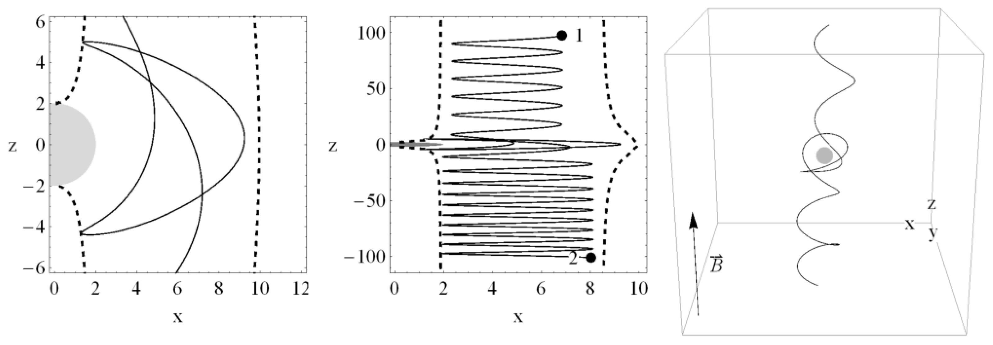
3.4.4. Modeling of Ionized Keplerian Disks around Magnetized Kerr Black Holes

For simplicity, we assume that the magnetic field lines are asymptotically parallel to the rotation axis of the Kerr black hole spacetime (i.e., to the vertical direction given by the z-axis) [23]. For the corotating Keplerian disk in the equatorial plane, a neutral test particle follows a circular geodesic corotating orbit with the covariant specific energy E and the specific axial angular momentum L given as [46]
E = a r - 3 / 2 - 2 r - 1 + 1 2 a r - 3 / 2 - 3 r - 1 + 1 , L = a 2 r - 3 / 2 - 2 a r - 1 + r 2 a r - 3 / 2 - 3 r - 1 + 1 .
However, the purely equatorial circular geodesic motion remains equatorial after ionization and is not entering the chaotic scattering regime, if there is no perturbation influence in the latitudinal (vertical) direction.11 In order to enter the chaotic scattering regime in the case of precisely equatorial disk, we have to assume its non-zero thickness allowing for an infinitesimal shift of the ionized particle in the perpendicular direction, or some infinitesimal impulsion in the perpendicular direction to the charged particles created by the ionization process. In fact, such a very small influence in the perpendicular direction can be caused by the irradiating photons.
On the other hand, it is natural to consider a Keplerian accretion disk having initially a very small but nonzero inclination to the equatorial (x-y) plane of the spacetime [33]—the slightly inclined disk represents another natural possibility to guarantee the entering to the chaotic scattering regime. The external uniform magnetic field remains aligned with the z-axis (vertical direction), being perpendicular to the equatorial plane of the spacetime.
Ionization of a neutral particle can be realized by irradiation of an atom by an incident photon resulting in an ion and electron, or we can consider a free neutron decay resulting in a proton and electron (plus an antineutrino, not considered here)—such a model corresponds naturally to the MPP [38,116] with the original 1st neutral particle being split into two charged particles—2nd and 3rd. Conservation of charge and canonical momentum of the particles entering the process reads
0 = q 2 + q 3 , π α ( 1 ) = π α ( 2 ) + π α ( 3 ) .
Of course, at the moment of ionization, the conservation of the kinetic momentum also holds
p α ( 1 ) = p α ( 2 ) + p α ( 3 )
as the electromagnetic contributions cancel each other out [10,33]. In the realistic scenarios considered here, i.e., the neutral atom ionization by irradiation or neutron β decay, one of the created charged particles is much more massive than the other one, say m 2 / m 3 1 , due to the mass ratio of proton to electron or ion to electron. The more massive charged particle clearly takes almost all the momentum of the original neutral particle and the dynamical influence of the lighter charged particle can be neglected
p α ( 1 ) p α ( 2 ) p α ( 3 ) .
Another realistic scenario is based on the idea of the accretion disk created by plasma considered as a quasi-neutral soup of charged particles, electrons and ions (protons), orbiting the black hole on circular orbits. For the matter of the disk dense enough, the main free path of the charged particles is very short in comparison with the length of the circular orbits, and the charged particles move collectively as a neutral body. Near the inner edge of the disk, the plasma density decreases substantially and the charged particles are not longer suppressed by their neighbours and start to move freely, being fully influenced by the electromagnetic field.
All the possible realistic ionization scenarios imply a simple model of ionized Keplerian disks based on the MPP process: a neutral particle becomes charged while its mechanical momentum remains conserved and starts to feel the influence of the electromagnetic field. This model was introduced in [33] where particle escape velocities and structure of escape zones were explored that were later studied also in [10,34,39]. This ionization model was also used to study the regular regime of the epicyclic oscillations [32] and its relation to the HF QPOs [22], or the fate of the Keplerian disks in dependence on the inclination angle in the case of non-rotating black holes [10,35].
The fate of the ionized Keplerian disks orbiting a magnetized Kerr black hole can be summarized describing the influence of the two basic parameters, the magnetic parameter ( B ) and the black hole spin a, on the fate of the ionized Keplerian disks, i.e., of the regular regime represented by the epicyclic motion, the regime of chaotic motion transforming the Keplerian disk into a toroidal accretion structure, destruction regime represented by direct infall of ionized matter into the black hole, and destruction jet regime represented by the escape of charged particles along the magnetic field lines to infinity. In the fourth case, the ultra-high energy particles (protons and ions) can be generated [39].
For the inclined Keplerian disk, we assume a special off-equatorial motion realized along the spherical trajectories with the orbit radius r 0 remaining constant, and with varying latitude θ . The ionization event can be thus assumed at some θ 0 π / 2 enabling the entering of the chaotic regime of the ionized particle motion—the charged test particle will be initially, at the ionization event, located on the spherical orbit with initial position x α and four-velocity u α
x α = ( t , r , θ , ϕ ) = ( 0 , r 0 , θ 0 , 0 ) ,
u α = ( u t , u r , u θ , u ϕ ) = ( E , 0 , 0 , L ) ;
the motion constants of the particle are governed by the specific energy E and specific angular momentum L of the electrically neutral particles following spherical orbits [117]
E = 1 S 1 - 2 r R 2 + a Q R 2 r sin θ ,
L = 1 S Q ( r 2 + a 2 ) r R 2 sin ( θ ) - 2 a r R 2 sin 2 ( θ ) ,
where the R 2 = r 2 + a 2 cos 2 θ and the functions Q , S are given by the relations
Q = r 2 - a 2 cos 2 ( θ ) ,
S = 1 - 3 r R 2 + 2 a Q R 2 r sin ( θ ) + a 2 R 2 r cos 2 ( θ ) .
Equations (134) and () reduce to the expressions for the specific energy and specific angular momentum of the equatorial geodesic circular (Keplerian) orbits (128) when θ = π / 2 . The inner edge of the spherically modified Keplerian disks is located at the innermost stable spherical orbit (ISSO) with radius implicitly given by
2 a Q r sin ( θ ) - 4 r 2 + ( r + 1 ) R 2 · Q 2 R 2 a 2 - 3 r 2 + 4 r 2 a 2 + r 2 - 2 r 2 R 2 a 2 + r 2 - 4 a Q 3 r 3 / 2 sin ( θ ) + 4 Q 2 r 2 - R 4 Q - a r sin ( θ ) Q a 2 + r 2 - 2 a r 3 / 2 sin ( θ ) = 0 .
This relation reduces for the motion confined in the equatorial plane to those governing the ISCO.
In order to consider situations relevant from the point of view of astrophysics, we assume the ionized part of the corotating Keplerian disks to be located near its inner edge, and we follow the fate of the ionized part by integrating motion of the charged particles in the background characterized by the magnetic parameter B and the black hole spin a. Typical examples of trajectories of the charged particles created by the ionization, initially orbiting on spherical orbits with radius r 0 > r ISSO , can be found in Figure 12, Figure 13, Figure 14 and Figure 15 constructed for characteristic values of the black hole spin a = 0.0.3.0.7.0.998 and for typical values of the magnetic parameter B = ± 0.001 , ± 0.01 , ± 0.1 , ± 1 , assuming the inclination of the Keplerian disk to be θ 0 = 1.5 . In the case of the magnetized Schwarzschild black holes and arbitrarily inclined Keplerian disks detailed results were presented in [10,35]. Here, we present the main results and differences between the situation around non-rotating and rotating black holes. The Keplerian disks are here assumed to be corotating with the Kerr geometry.
Contrary to the Schwarzschild case with a = 0 where the canonical energy remains the same as the kinetic energy, for the magnetized rotating black holes there is a shift in the canonical energy governed by the non-zero A t component of the electromagnetic potential that allows escaping of the charged particle to infinity along the magnetic field lines – the acceleration due to the electric component of the electromagnetic field can be enormous [33,38]. For example, the escaping particles can undergo extremely efficient MPP reaching an ultra-high energy of the order of 10 21 eV, if the process of acceleration occurs near a supermassive black hole having mass M 10 10 M surrounded by magnetic field of the order of 10 4 G [10,39,81].
In the case of magnetized Schwarzschild black holes ( a = 0 ) the situation is illustrated in Figure 12. Here, and, in the following figures representing the disk fate, the uncharged test particles on innermost stable spherical orbit (the dashed circle) represent the inner edge of the Keplerian accretion disk; the fate is studied for a region close to the inner edge. For the disk that remains neutral, or for the vanishing magnetic field ( B = 0 case), all the orbits keep the original form and the inclined razor thin disk remains. For a weak electromagnetic interaction switched-on ( B = ± 0.001 cases), the charged particles enter epicyclic oscillatory motion around the circular orbit in both radial and latitudinal directions, only particles forming the innermost region are captured by the black hole in the case of magnetic attraction ( B = - 0.001 ); the accretion disk becomes slightly thicker due to the vertical epicyclic motion. For stronger electromagnetic interactions switched-on ( B = ± 0.01 , ± 0.1 cases), the charged particles enter a fully chaotic regime or they fall directly to the black hole; the accretion disk is destroyed, partly destroyed, or transformed into thick toroidal structure. The complete destruction of the inner region of the Keplerian disk occurs in the B = - 0.01 case, when all the particles are captured by the black hole, a large part of the charged particles are captured for B = - 0.1 , the rest enter chaotic motion. If large electromagnetic interaction is switched-on ( | B | 1 cases), the Lorentz force dominates the particle motion. The charged particles can enter a special regime of the regular motion due to spiraling up and down along the magnetic field lines due to fast Larmor oscillations combined with slow motion around the black hole in the clockwise ( B > 0 ) or the counterclockwise ( B < 0 ) direction, demonstrating vertical oscillations—in this case, the thin Keplerian disk transforms into a special toroidal structure.
In the case of slowly rotating black holes ( a = 0.3 ) illustrated in Figure 13, the situation remains very similar to the Schwarzschild case for the weak and mediate values of the magnetic parameter of charged particles with an exception of the mediate repulsive magnetic parameter with B = 0.1 when an increase of the particle canonical energy due to electric acceleration causes the overcoming of the repulsive centrifugal barrier and capturing of the innermost ionized particles by the black hole. For the large magnitudes of the magnetic parameter, the behavior of the ionized part of the disk becomes dramatically dependent on the sign of the magnetic parameter B . For the negative values ( B = - 1 case), the character of the motion remains similar to those corresponding to the Schwarzschild black holes, but, for positive values ( B = 1 case), the influence of the magnetic field is getting stronger with increasing radius of the original orbit causing increase of the amplitude of the vertical oscillatory motion.
For black holes with mediate spin ( a = 0.7 ), the results are illustrated in Figure 14. Now, the fate of the inner part of the disk is similar to the case of slow rotation, but the effects of black hole spin are amplified—namely, for the case of mediate positive values of the magnetic parameter, B = 0.1 increase of the particle canonical energy due to electric acceleration causes entering of the chaotic motion creating winds in the innermost region of the disk. For the large positive values of the magnetic parameter ( B = 1 case), the combined influence of the black hole spin and the magnetic field implies escape of all the considered particles to infinity along the magnetic field lines with the exception of those originating almost at the ISSO that remain in oscillatory motion in the vertical direction combined with the Larmor orbital motion with very small radii.
For near-extreme rotating black holes ( a = 0.998 ), the fate of the Keplerian disks is demonstrated in Figure 15. The near-extreme spin now causes the decrease of charged particles from the innermost regions of the disk for both large and mediate negative values of the magnetic parameter (cases B = - 0.1 , - 1 ), but the infall of the particles is stopped in the case of slightly negative magnetic parameters (case B = - 0.01 ). For the large positive magnitudes of the magnetic parameter (case B = 1 ), charged particles from whole the ionized region escape to infinity, those from the innermost part of the disk are executing a period of chaotic motion before the escape.
We can summarize that the increasing spin of the black hole for fixed magnetic parameters causes increasing influence of the electromagnetic field due to an increase of its electric component. For low values of the magnetic parameter, the increasing spin generally implies increasing chaotic character of the motion, but it can be transmuted to particle capture by the black hole for particles sufficiently close to the ISCO if the particle canonical energy overcomes the repulsive centrifugal barrier. The most interesting situation occurs for values of the magnetic parameter B ± 1 , as in this case around slowly rotating black holes with a 2 0 , for both negative and positive values of the magnetic parameter, an interesting regular type of the motion arises, demonstrating the Larmor rotation around the magnetic field lines mixed with a slow orbital motion combined with a quasi-geodesic “epicyclic” vertical and radial oscillatory motion. For B - 1 , this kind of motion survives with increasing spin. For B 1 , increasing spin implies increasing amplitude of the vertical oscillatory motion and possible tendency of the particles to escape to infinity; moreover, for large values of the spin ( a > 0.7 ), the orbits in close vicinity of the black hole horizon demonstrate increasing degree of chaos. With magnetic parameter B increasing above the unit value, the particles escape to infinity and the region of chaotic motion starts to be more and more restricted. In the next section, we concentrate on the case of acceleration and motion of the escaping particles discussing in detail the MPP.

3.5. Magnetic Penrose Process and Creation of Jets

As the MPP is a local decay processes, its energy balance is governed by the local value of the electromagnetic field (potential) and the simple approximation of asymptotically uniform magnetic field aligned with the rotations axis can be applied. We consider now the MPP with inclusion of decaying charged particles. For simplicity, we restrict to the case of the equatorial motion assuming small impulsion in the vertical direction that guarantees entrance to the chaotic regime necessary for escape to infinity along magnetic field lines, but for the energetic balance during the decaying process, the equatorial restriction is used giving potentially highest efficiency of the MPP process. For the stability of the equatorial motion in the Kerr spacetimes against vertical perturbations, see [60,118].
The charged particle motion is determined by the spacetime geometry and the electromagnetic potential. For the equatorial motion around a magnetized Kerr black hole, the effective potential giving turning points of the radial motion of the particle with the canonical energy E and the canonical angular momentum L takes the form
V eff = - q A t - g t ϕ g ϕ ϕ L + - g t t + g t ϕ 2 g ϕ ϕ L 2 g ϕ ϕ + 1 ,
containing a non-zero time component of the electromagnetic potential that guarantees extension of possible negative energy states across the ergosphere whose outer boundary is most extended in the equatorial plane being located at the stationary radius r s = 2 —around a magnetized black hole, the effective ergosphere allowing existence of negative energy states and extraction of the energy from the black hole can be extended with no limit [61,119].
We thus consider splitting of the 1st particle (generally positively charged, but its neutrality is not excluded) onto two charged particles, the 2nd one having a positive charge and the 3rd one having a negative charge. If one of the particles (say the 3rd one) has a negative canonical energy E 3 < 0 , then the second one should have the canonical energy E 2 > E 1 due to an extraction of the black hole energy because of the capture of the 3rd particle. The process of the split of the 1st particle into the 2nd and 3rd ones is governed by the conservation of the electric charge
q 1 = q 2 + q 3 ,
and the conservation of the canonical momenta
π α ( 1 ) = π α ( 2 ) + π α ( 3 ) .
The orbital motion of the charged particles can be characterized by their angular velocity related to the static observers at infinity given by the relation
Ω = d ϕ d t = u ϕ u t .
The angular velocity of the charged particles is restricted by the null vector limits on the 4-momentum p α that are given by the metric coefficients due to the relation
Ω ± = 1 g ϕ ϕ - g t ϕ ± g t ϕ 2 - g t t g ϕ ϕ .
The canonical (conserved) energy of the 2nd, escaping particle can be expressed in the form [39]
E 2 = χ ( E 1 + q 1 A t ) - q 2 A t ,
where
χ = Ω 1 - Ω 3 Ω 2 - Ω 3 X 2 X 1 , X i = g t t + Ω i g t ϕ ,
where Ω i ( X i ) is the angular velocity (the velocity factor) of the i-th particle. The MPP requires the electromagnetic term - q 2 A t to be positive and playing dominant role. For q 2 > 0 and B > 0 , a > 0 the condition - q 2 A t < 0 is satisfied due to definition of A t , its dominant role is guaranteed by large values of the magnetic parameter B . Escape to infinity is realized through the chaotic scattering process [33].
The energy of the second particle (e.g., proton) E 2 = p t 2 + q A t can be thus very large, while energy of the third particle E 3 = p t 3 - q A t can be negative with very large magnitude (or vice versa, for dependence on the orientation of the magnetic field lines). The process of the chaotic scattering, discussed in [33], then guarantees that the highly energetic second particle escapes to infinity along the magnetic field lines; the third particle with large negative energy is immediately captured by the black hole, as demonstrated in Figure 16.
The same MPP process of charged particle acceleration is demonstrated in Figure 17 and Figure 18, but for different values of magnetic field parameter B . We can see no particle escape in the case of low magnetic field B parameter (Figure 17) while escape with large velocity in the case of high magnetic field B parameter (Figure 18).

3.5.1. Efficiency of the Magnetic Penrose Process and Its Three Regimes

The efficiency of the MPP is defined in the standard way relating the gained and input energies
η = E 2 - E 1 E 1 = - E 3 E 1 ,
implying the relation
η MPP = χ - 1 + χ q 1 A t - q 2 A t E 1 .
All the quantities are taken at the splitting point; the angular velocity of the particles created by the splitting process is restricted by the relation
Ω - Ω Ω + .
The limiting cases govern the maximal possible efficiency of the process.
The MPP can enter three regimes demonstrating substantially different efficiency. The first, low efficiency regime, corresponds to the original Penrose process involving only electrically neutral particles (or vanishing electromagnetic field). In this case, the maximal efficiency can be established using the limiting values of the angular velocity and reads [80]
η PP ( max ) = 2 - 1 2 0.207 .
Note that in this low efficiency regime the efficiency is even lower than the efficiency of the Keplerian accretion process for near-extreme Kerr black holes ( η 0.427 ) [120], or the near-extreme Kerr naked singularities ( η 1.573 ) [47,48].
The second, moderate regime of the MPP corresponds to the situation when the electromagnetic forces are dominant, i.e., the condition | q m A t | > > | u t | is satisfied. In the moderate regime, the efficiency is approximately determined by the relation
η M P P m o d q 2 q 1 - 1
that operates while q 2 > q 1 ; the gravitationally induced electric field of the black hole is thus neutralized. The moderate regime of the MPP is close to the Blandford–Znajek process [42]; both processes are driven by the quadrupole electric field generated due to twisting the magnetic field lines because of the spacetime frame dragging, and restricted by global neutrality of the plasma surrounding the black hole [38].
The third, extremely efficient regime corresponds to ionization of neutral matter and its efficiency is dominated by the term
η MPP extr q 2 m 1 A t .
In the extreme regime of the MPP, an enormous increase of the efficiency is possible, giving enormous energy to escaping particles. In such a case, the efficiency can be as large as η MPP extr 10 10 if the magnetic field is sufficiently large and the rotating black hole is supermassive. For such extremely large efficiency, the black hole rotation is necessary, but, contrary to the Blandford–Znajek process, it is not necessary to have a near-extreme black hole. The dependence of the particle energy reflecting the efficiency on the black hole mass and the spin and the magnetic parameter is illustrated in Figure 19.
The critical point for the extreme regime of the MPP process is the electric neutrality of the incident particle that should reach the region very close to the horizon where the acceleration can be efficient and space free of matter enabling, thus the charged particle escapes to infinity after its chaotic scattering. Notice that the case of the ionized Keplerian disks fulfills well these conditions, as we can write
π α ( 1 ) = π α ( 2 ) + π α ( 3 ) , p α ( 1 ) = p α ( 2 ) + q A α + p α ( 3 ) - q A α ,
m ( 1 ) m ( 2 ) + m ( 3 ) , 0 = q ( 2 ) + q ( 3 ) ,
and, using the assumption that the third particle has mass much smaller than the second one,
m ( 1 ) m ( 2 ) m ( 3 ) ,
we can assume
p α ( 1 ) p α ( 2 ) p α ( 3 ) .
The MPP is simplest for the ionized Keplerian disks as the splitting electrically neutral particles follow purely circular orbits. In this case, the 2nd particle is escaping with large canonical energy E ( 2 ) = p t ( 2 ) - q ( 2 ) A t , while the 3rd particle is captured with large negative energy E ( 3 ) = p t ( 3 ) - q ( 3 ) A t = p t ( 3 ) + q ( 2 ) A t .
Moreover, the MPP combined with the process of chaotic scattering transmuting the nearly circular motion of charged particles of the ionized Keplerian disks orbiting the magnetized Kerr black holes to the linear motion along the magnetic field lines parallel to the black hole axis, can well serve as a simple model of creation of strongly relativistic jets observed in many active galactic nuclei and quasars—the external magnetic field serves as a catalyst for the acceleration of the created charged particles and extraction of the rotational energy due to captured negative-energy charged particle, and simultaneously the magnetic field lines orthogonal to the disk plane could serve as an efficient collimator of the particle motion. In the regions of very low density located under the inner edge of the equatorial accretion disk, the charged particles having the highest possible energy could survive their travel to the distant observers, being held by the magnetic field lines very close to the black hole rotation axis.
Using the exact expressions for the electromagnetic potential of the asymptotically uniform magnetic field in the vicinity of the Kerr black hole, we obtain for the splitting process in the equatorial plane the efficiency of the MPP in the extreme regime in the form (using now the standard units)
η MPP extr = 1 2 r s / r s p - 1 + q 2 G B M a m 1 c 4 1 - r s 2 r s p ,
where B is the magnetic field intensity, r s = 2 G M / c 2 is the static limit radius (boundary of the ergosphere) at the equatorial plane, and r s p is the radius of the splitting point located between the black hole horizon and the stationary limit radius. The first geometrical term reflects the efficiency of the Penrose process and reaches maximum of η P P = 0.207 . The relevant one is the second term giving contribution of the electromagnetic acceleration—this term exceeds the “annihilation” value of η = 1 in the case of electrons accelerated by a stellar mass black holes with magnetic field B m G . Clearly, it must be enormously large for the supermassive black holes and strong magnetic fields. We also see directly that the Penrose process governed by the first part of the RHS of the equation giving the extreme regime efficiency is restricted to the ergosphere, i.e., close vicinity of the black hole horizon, while the electromagnetic part is not, as the effective ergosphere has no limit in this case. This fact enhances the astrophysical applicability and relevance of the MPP.
In order to make a comparison of the moderate and extreme efficient MPP, we consider two similar splitting processes that occur around a Kerr black hole of mass M = 10 M and spin a = 0.8 , immersed in a magnetic field of intensity B = 10 4 G . The processes are represented by electron loss by a charged and uncharged Helium atom:
He α ( He + + ) + 2 e - , He + α ( He + + ) + e - .
Then, the efficiency of the extremely efficient MPP reads
η He extr = 2.4 × 10 3 ,
while, for the moderate MPP, we obtain
η He + mod = 0.99 .
Clearly, the split charged particles give efficiency only of the order 1, while significantly higher efficiency can be obtained for electrically neutral particles reaching in our case order of 10 3 —we can immediately see that, for supermassive black holes observed in some galaxies to have mass M 10 10 M with surrounding magnetic field B 10 4 G, the efficiency can grow up to η MPP extr 10 12 [39].
If the MPP is related to ionized Keplerian disks in connection with the chaotic scattering process, we can conclude that, in the case of magnetized rotating black holes, it can lead to creation of jets escaping to infinity with high velocities due to the extraction of rotational energy of the black holes because of the captured electrons of high negative energy, being thus a basic process for more complex Blandford–Znajek processes [38]. If the ionized disk is orbiting a non-rotating black hole (or slowly rotating black hole surrounded by a weak magnetic field), the MPP processes generate winds that are not escaping to infinity, with energy coming from the rotational energy of the orbiting matter (representing the Payne–Blandford process [121]). Note that the transmutation of the rotational energy of the matter originally orbiting in the Keplerian disk is present also in formation of jets due to the chaotic scattering process, but the energy related to this transmutation of energy of the orbital motion to the energy of the translational motion is small in comparison with those corresponding to the acceleration by the electromagnetic field.

3.5.2. Ultra-High Energy Cosmic Rays as Products of MPP in the Extreme Regime

The cosmic rays are detected with large extension of the particle energy. The cosmic rays are usually constituted by high-energy protons or ions; observed isotropic distribution indicates an extra-Galactic origin and the model of their creation is under long debate. Of special interest are observations of the Ultra-High-Energy Cosmic Rays (UHECRs) corresponding to particles having the energy E > 10 18 eV—occasionally, even particles with energy exceeding E > 10 21 eV are observed, overcoming the GZK limit of 10 19 eV due to interaction with the cosmic microwave background.
Now, we have to estimate applicability of our acceleration MPP model to explain the UHECRs reaching in the case of observed protons or ions the energy E 10 20 eV related to the GZK limit of E 10 19 . 7 eV connected to the interactions with photons of the cosmic microwave radiation, and reaching in some exceptional case even the energies overcoming E 10 21 eV. Recall that the energy loss determined by the GZK-cutoff restricts strongly the distance of sources giving cosmic rays with energy overcoming this energy cutoff putting the limiting distance to l 100 Mpc [122]. The results obtained by the Pierre Auger Observatory indicate correlation of the arrival direction of the ultra-high energy particles with E > 10 20 eV to the active galactic nuclei at the distances lower than 100 Mpc.
Considering the MPP creating protons due to the neutron beta decay, or ions because of the ionization of electrically neutral atoms starting at H through He up to Fe, we are able to explain the UHECR energies quite naturally for magnetized supermassive black holes. The maximum of the energy of a charged particle created in the MPP working in the extremely efficiency regime can be predicted in a precise way to be given (in physical units) as
E MPP = 1.3 × 10 21 eV q e m p m a B 10 4 G M 10 10 M .
This dependence is illustrated in Figure 19. Clearly, the protons with energy E > 10 21 eV can be created even by mildly spinning (say a 0.8 ) supermassive black holes with mass M = 10 10 M immersed in magnetic field of strength B = 10 4 G. The maximum energy corresponding to ions generated in the vicinity of the given black hole is slightly modified, being lowered according to the the ratio of proton mass and the mass of considered ions.
A special position in generation of the high-energy particles observed by the Pierre Auger Observatory has to be related to the Galaxy center SgrA* black hole—as this is the closest supermassive black hole, the particles accelerated in its vicinity have to observed frequently. Its mass is determined by observations of stars orbiting around the black hole to be M SgrA * 4.14 × 10 6 M [123], its spin is estimated to be a SgrA * 0.5 [124], and the magnetic field in its vicinity is estimated to be B 10 G [125] but an increase by one order to 100 G is possible [86]. Therefore, the maximal energy of protons generated near the horizon of SgrA* black hole can be expressed in the form
E p - SgrA * = 10 15 . 6 eV q e m p m B 100 G a 0 . 5 M 4 . 14 × 10 6 M .
It is quite interesting that this value just coincides with the so-called knee of the energy spectrum in the observed data, located at E knee 10 15 . 6 eV, where the number of the observed particle flux is significantly suppressed, indicating existence of a strong single source located at a relatively short distance. The MPP applied to the SgrA* thus indicates an idea to relate the model to the knee of the UHECR data at E 10 15 . 6 eV. This idea requires a detailed study related to statistics and directionality of data connected with the knee. We can also note that the maximal proton energy E MPP 10 19 eV can be generated around the supermassive black hole in the M87 galaxy having mass M = 7 × 10 9 M and magnetic field strength B = 10 2 .
If protons can be accelerated to the maximal energy E 10 21 eV, in the case of accelerated electrons, we could obtain energy larger by the factor of m p / m e 1820 , i.e., as high as 10 24 eV that is not observed. Explanation of this fact will be presented in the next section, being based on the efficiency of the deceleration of the charged particle motion due to back-reaction to the electromagnetic (synchrotron) radiation of the charged particles in the magnetic field near the black hole, or all the way along its way to the observer. A question arises as to whether the MPP acceleration model could be related to neutron stars, especially magnetars. In fact, some estimates can be made, as we have demonstrated in [10] that the ionization process in vicinity of a given radius r is similar for the asymptotically uniform (Wald) magnetic field and the dipole magnetic field that can be relevant for magnetars. Furthermore, the internal and external gravitational field of neutron stars can be modeled for a slow rotation neutron star by exact general relativistic numerical codes, e.g., LORENE [126,127], or by approximative Hartle–Thorne models where both internal and external geometry is constructed as perturbative modification of the spherically symmetric static solutions considered to the 2nd order of angular velocity of the star assumed to be in rigid rotation [128]. The external Hartle–Thorne geometry can be then characterized by mass M, angular momentum J and quadrupole moment Q. It has been shown that the exact numerical models and external Hartle–Thorne geometry give very similar spacetime structure for models with dimensionless spin a = J / M 2 = 0.4 and can be thus applied to almost all of the observed neutron stars [129,130,131]. The external Hartle–Thorne geometry exactly corresponds to the Kerr geometry, if the dimensionless quadrupole moment q Q M / J 2 = 1 , and they can be very close if q 2 [131,132]. The neutron star with q 2 are very massive and compact stars, near the maximum mass allowed by considered equation of state. For such massive neutron stars, the Kerr geometry can be applied and, due to the rotational effect, the quadrupole electric field is generated in relation to the magnetic dipole field that can serve in the MPP analogously to Kerr black hole case. There, the energy E 10 21 eV could be obtained by protons near the rotating massive magnetars, as their mass decrease of 10 orders to M 2 M is just compensated by increase of the magnetic strength to 10 14 G, but, in this case, the radiation back-reaction is even much more efficient in comparison with the case of supermassive black holes with substantially weaker magnetic fields.

3.5.3. Synchrotron Radiation of Accelerated Charged Particles

Any charged particle moving in an electromagnetic field emits synchrotron radiation [133], causing the appearance of the back-reaction force which can significantly affect its motion. In order to detect the ultra-high energy charged particles (protons, ions, or electrons) by observers at large distances from the magnetized black holes, the back-reaction force effect along the particle trajectory has to be small or negligible. We thus now estimate the back-reaction of the synchrotron radiation in the vicinity of the magnetized black hole where the magnetic field strength is comparable to those at the splitting point. We thus study the charged particle motion in the combined magnetic and gravitational fields, including the influence of the radiation reaction force f R μ in addition to the standard Lorentz force. In the non-relativistic limit, the back-reaction force related to the synchrotron radiation is given by the formula f R = 3 q 2 2 m d 2 u α d τ 2 , and this force must satisfy the condition of orthogonality to the 4-velocity, i.e., f R μ u μ = 0 . The covariant form of the back-reaction force vector takes the form
f R μ = 2 q 2 3 m d 2 u μ d τ 2 + u μ u ν d 2 u ν d τ 2 .
In the framework of relativistic physics, the charged particle motion is governed by the Lorentz–Dirac equation reflecting through the Lorentz force the direct influence of the external electromagnetic fields, and, through the related radiation–reaction force, the influence of the synchrotron radiation generating a secondary electromagnetic field—the radiation back-reaction force arises from the radiative field of the charged particle. In general form, the equations of motion take the form
D u μ d τ = q ˜ F ν μ u ν + q ˜ F ν μ u ν .
The first term on the right-hand side of Equation (163) is the Lorentz force related to the electromagnetic tensor F μ ν of the external electromagnetic field, here assumed to be an asymptotically uniform magnetic field, the second term is the back-reaction self-force related with the radiative field F μ ν = A ν , μ - A μ , ν of the moving charged particle. The vector potential of the particle self-electromagnetic field satisfies the wave equation
A μ - R ν μ A ν = - 4 π j μ ,
where = g μ ν D μ D ν , and D μ is the covariant differentiation, R ν μ is the Ricci tensor of the spacetime. The vector potential of the self-field can be expressed as a retarded solution of Equation (164)
A μ ( x ) = q G + λ μ ( x , z ( τ ) ) u λ d τ ;
G + λ μ is the retarded Green function, integration is taken along the worldline of the particle z ( τ ) , thus u μ ( τ ) = d z μ ( τ ) / d τ [134].
For curved spacetimes, the fully general relativistic form of the dynamics of a radiating charged particle was introduced in [135] and completed in terms of tetrad formalism in [136]. The explicit form of Equation (163) in curved spacetimes takes the form
D u μ d τ = q ˜ F ν μ u ν + 2 q 2 3 m D 2 u μ d τ 2 + u μ u ν D 2 u ν d τ 2 + q 2 3 m R λ μ u λ + R λ ν u ν u λ u μ + 2 q 2 m f tail μ ν u ν ;
the last term of Equation (166) is the so-called tail integral governed by the Green function [134,136]
f tail μ ν = - τ - 0 + D [ μ G + λ ν ] z ( τ ) , z ( τ ) u λ d τ .
The tail integral is calculated over the past history of the charged particle—primes indicate its prior positions—all the other quantities are evaluated at its current position z ( τ ) . The Ricci tensor vanishes in the vacuum spacetimes, as is the case of Kerr spacetime, so the terms containing the Ricci tensor are irrelevant in our considerations. The “tail” integral in (166) implies that the radiation reaction in curved spacetimes has non-local nature, as the charged particle motion depends on its whole history, not solely on its current state. The radiation field F μ ν in Equation (163) of the moving charged particle interacts with the spacetime curvature being reflected back to the particle due to the curvature barrier, with a time delay governed by the tail integral (166). The radiated electromagnetic field of a charged particle thus carries information about the particle history.
The relevance of the tail term can be estimated (see [137,138] and subsequent papers). For a particle with the charge q and mass m, the ratio of the tail force F tail G M q 2 / ( r 3 c 2 ) to the Newton-force F N G M m / r 2 in the vicinity of a black hole ( r r H = 2 G M / c 2 ) of the stellar mass M 10 M is
F tail F N q 2 m M G 10 - 19 q e 2 m e m 10 M M ,
where e and m e are the charge and the mass of an electron, while, for supermassive black holes (SMBH) ( M 10 9 M ), this ratio is even by eight orders lower. Therefore, in situations corresponding to the non-relativistic, or moderately relativistic motion with the Lorentz factor smaller than unity, the tail term can be surely neglected. The analysis of the cases with the relativistic or ultra-relativistic motion with the Lorentz factor larger or much larger than unity [139,140] implies the conclusion that for any particle moving with relativistic velocity the tail term is negligible in comparison with the electromagnetic radiation reaction force [36].
Therefore, the equation of motion (166) can be reduced to the form of the covariant Lorentz–Dirac equation:
D u μ d τ = q ˜ F ν μ u ν + f R μ ,
with the radiation reaction force
f R μ = 2 q 2 3 m D 2 u μ d τ 2 + u μ u ν D 2 u ν d τ 2 .
Using the four-acceleration a μ = D u μ / d τ , we can rewrite the term D 2 u μ / d τ 2 in the form
D 2 u μ d τ 2 D a μ d τ = d a μ d τ + Γ α β μ u α a β , = d d τ d u μ d τ + Γ α β μ u α u β + Γ α β μ u α d u β d τ + Γ ρ σ β u ρ u σ , = d 2 u μ d τ 2 + Γ α β μ x γ u γ u β + 3 Γ α β μ d u β d τ + Γ α β μ Γ ρ σ β u ρ u σ u α .
The Lorentz–Dirac equations are plagued by the runaway solutions [36]—these can be avoided by reducing the order of the differential equations. Applying the covariant derivative with respect to the proper time to both sides of the Lorentz equation, we arrive at
D 2 u α d τ 2 = q ˜ D F β α d x μ u β u μ + q ˜ 2 F β α F μ β u μ .
Then, we obtain the radiation reaction force in the form
f R α = k q ˜ D F β α d x μ u β u μ + q ˜ F β α F μ β + F μ ν F σ ν u σ u α u μ ,
with
D F β α d x μ = F β α x μ + Γ μ ν α F β ν - Γ β μ ν F ν α .
Equations (169) and (173) represent the covariant form of the Landau–Lifshitz equations.
Detailed analysis of the particular case of the motion of charged particles around a Schwarzschild black hole immersed into an external asymptotically uniform magnetic field was presented in [36], where the equations of motion are given in separated form and the results of their numerical integration are obtained in typical situations; the special case of the widening of circular orbits was discussed in [37]. Effect of radiation reaction on charged particle dynamic around rotating Kerr black hole can be seen in Figure 20. Here, we summarize the implications for the covariant energy and axial angular momentum due to the radiation force.
The energy-momentum radiated by a charged particle is determined by the integral of the radiation reaction force along the particle worldline. In the flat spacetime, the radiated four momentum of a particle with charge q is given by d P μ / d τ = 2 3 q 2 a α a α u μ [133]. In curved spacetimes, the synchrotron radiation has been studied in [141,142] using covariant form of the flat space results; the problem has been revisited recently in [143]—however, without consideration of the radiation reaction force.
The evolution of the particular four-momentum components of the particle influenced by the radiation reaction force is governed by Equations (169) and (173). Restricting for simplification to the equatorial motion, the energy loss can be given as [36]
d E d τ = - 2 k B 2 B E 3 - E 2 B f + u ϕ r ,
and the rate of the angular momentum loss reads
d L d τ = 4 B 2 k u ϕ f 2 ( u t ) 2 - f - 2 u r u ϕ r - 4 B 2 k 2 + 2 r B u r .
Detailed study of the energy and angular momentum losses implied by numerical integration of the equations of motion with the radiation reaction term, without the restriction to the equatorial plane, is presented in [36]. Here, we concentrate on the case of damping of ultra-high energy particles.

3.5.4. Proton and Electron Energy after Leaving the Vicinity of Magnetized Black Holes

For ultra-high-energy relativistic particles, with E 1 , the most relevant contribution to the energy loss is given by the first term in square brackets of (175). The crucial information is given by the relaxation time τ required for decay of the radial oscillatory motion of a charged particle due to the radiation reaction force. Of course, its calculation is relevant only when the radiation reaction is not leading to the particle fall into the black hole, i.e., for particles escaping or oscillating near the circular orbit. The rate of the energy loss can be related to the relaxation time as
E ˙ = E f - E i τ ,
where E i ( E f ) denote the initial (final) energy of the particle. For ultrarelativistic particles, with velocity v c , the energy loss is governed by the first term of the expression (175), which gives
d E d τ = - 4 B 2 k E 3 .
Its solution can be expressed in analytic form
E ( τ ) = E i 1 + 8 B 2 k E i 2 τ ,
with E i being the initial energy. The relaxation time τ governed by (179), related to the final energy E f , can be expressed as
τ = 1 4 k B 2 E i 2 - E f 2 E i 2 E f 2 .
For the case of epicyclic oscillatory motion around non-rotating black holes [31], we can easily estimate the relaxation time required for decrease of the maximal energy at the bounded (unstable circular) orbit corresponding to the maximum of the effective potential to the lowest energy corresponding to the minimum of the effective potential at the stable circular orbit. Therefore, we identify the energy limits such that E i = E + and E i = E - , where the energy E + ( E + ) corresponds to the unstable (stable) circular orbit and is given by
E ± 2 = r f 2 ( r - 3 ) 2 r - 3 + 2 B 2 r 3 f ± 2 B r r - 3 + B 2 r 4 f 2 ,
where the signs correspond to the maximal and minimal energy of a particle at the circular orbit, and f = 1.2 / r is the lapse function. The difference between E + and E - can be large for large values of the magnetic parameter B , representing the charged particles accelerated up to ultrarelativistic velocities [31,33]. For large values of B , the locations of the effective potential extrema giving the stable and unstable circular orbits are very close [31]; therefore, we can assume r max E r min E = r and the relaxation time can be expressed in the form
τ max = r - 3 + B 2 f 2 r 4 k B 1 + 4 B 2 r 2 f 2 .
For large values of the magnetic parameter B , we can simplify Equation (182) to the simple form
τ max 1 k B 2 f ( r ) , B 1 .
We see that, due to presence of the lapse function, the relaxation time increases while the radius r approaches the black hole horizon, i.e., the decay of the oscillatory motion is slower if the particle is orbiting closer to the black hole. However, for insight into astrophysical processes, the factors characterizing the moving particle are crucial: the black hole parameters and the magnetic field strength.
To relate our models to realistic astrophysical scenarios, we estimate the relevant parameters—first the magnetic interaction parameter B governing the acceleration of particles, then the relaxation time τ governing the decay of the particle energy.
Restoring the world constants, the dimensionless parameter B reflecting the relative influence of the gravitational and magnetic fields on the charged particle motion takes the form
B = | q | B G M 2 m e c 4 .
The characteristic values of the magnetic fields near the stellar mass and supermassive black holes are B 10 8 G for M = 10 M , and B 10 4 G for M = 10 9 M [144,145]. For electrons, we thus find
B BH 4 . 32 × 10 10 for M = 10 M ,
B SMBH 4 . 32 × 10 14 for M = 10 9 M .
As a relevant example, we can consider the vicinity of the supermassive black hole at the Galaxy center SgrA*. The equipartition strength of the magnetic field near the Milky Way center is established to be of tens of Gauss ([146]). Moreover, the multi-frequency measurements of pulsar orbiting near the Galaxy Center [86] demonstrate existence of a strong magnetic field of a few hundred Gauss near the black hole event horizon. The mass of the SgrA* black hole candidate is estimated to be 4.2 × 10 6 M (for more details about Sgr A*, see [125]). Thus, the magnetic parameter B for the electrons orbiting the SgrA* black hole can be estimated as
B SgrA * | e | B G M 2 m e c 4 1.86 × 10 10 .
For protons, the values of B in (185)–(187) are lowered by the factor m p / m e 1836 . The extremely large values of the parameter B in realistic astrophysical scenarios imply that the effects of magnetic field on the dynamics of charged particles play a crucial role.
The influence of the radiation reaction force on damping of the charged particle energy is represented by the relaxation time τ containing along with the magnetic parameter ( B ) also the parameter k expressed in dimensionless form in terms of the particle parameters and black hole mass
k = 2 3 q 2 m G M .
The parameter k is much lower than the magnetic parameter B in realistic situations. For example, in the case of electrons orbiting stellar mass and supermassive black holes, we obtain
k BH 10 - 19 for M = 10 M ,
k SMBH 10 - 27 for M = 10 9 M .
For example, electrons orbiting the Sgr A* black hole have k SgrA * 10 - 25 . For protons orbiting in the same conditions as electrons, the k parameter is lower by the factor m p / m e 1836 , similarly to the case of the magnetic parameter B .
Although the values of the parameter k are very low as compared with values of the parameter B , the damping of the particle energy due to the radiation reaction force can be very strong because the relaxation time depends quadratically on the magnetic parameter B that can be extremely large around magnetized black holes. In Table 5, we present results of calculations of the relaxation time for electrons and protons orbiting in the same conditions a black hole, assuming uniform magnetic fields with values of the magnetic field strength B covering large variety of situations relevant in astrophysics. We can confront these results with the particle orbital timescale τ c for the stellar mass and supermassive black holes—assuming the ISCO, we obtain
τ c 10 - 3 s , for M = 10 M ,
τ c 10 4 s , for M = 10 9 M .
For the widely discussed Sgr A* supermassive black hole, we find the electron decay time 10 4 s, while the orbit time at ISCO takes the value 10 3 s, i.e., the timescale of the energy decrease is in this case by one order larger than the orbital time.
We can see that, with dependence on the astrophysical conditions and the type of the charged particle, the relaxation time of energy decay covers an extremely large range. We can immediately see that the differences between the characteristic relaxation times for electrons and protons differ very strongly—due to the large ratio of their masses, m p / m e 1836 , and the dependence
τ m 3 q 4 B 2 ,
we find the enormous value of the ratio τ p / τ e 10 10 . We can thus see that electrons are in fixed conditions accelerated with efficiency 10 3 larger than protons, but their energy decays with efficiency 10 10 larger than proton energy. Similarly, the energy due to acceleration by the electromagnetic field depends linearly on B, but decay of the energy due to radiative reaction force depends on B 2 . Therefore, charged particles can be accelerated to the same energy around supermassive black holes with M 10 10 M immersed in the field of B 10 5 G , and magnetars with M M immersed in the field of B 10 15 G , but, around such magnetars, the particles’ energy decays with efficiency 10 10 higher so we cannot see the extremely energetic particles coming from magnetars, but we can see them in the case of supermassive black holes. As can be seen from relation (193), the differences in the acceleration and energy decay processes can be important also in the case of ions—in this case, the modifications of the various ion mass in relation to the proton mass can be relevant in estimations of the acceleration and energy decay processes, but also the degree of ionization can make an important contribution to the outcomes of these processes.
We expect that the imprints of the acceleration MPP and the related energy decay process, determined by conditions around the magnetized black hole, along with the energy decay processes connected with the intergalactic travel of the ultra-high energy protons and ions, could give relevant information enabling localization of the sources of such particles, if the observational data are sufficient. An elementary test of this kind is calculation of the energy decay due to the radiation reaction forces for ultra-high energy ( E > 10 20 eV) charged particles moving in very large distances through a very weak magnetic field of B 10 - 5 eV representing an intergalactic field—the results demonstrate that the particle energy E < 10 21 eV can survive to distance l 100 Mpc, which is comparable to the distance corresponding to the so-called GZK limit; on the other hand, the particle energy E 10 22 eV can survive to the distance l 10 Mpc [39].
One can estimate the timescale of the decay of charged particle oscillations. Typical orders of magnitude of the oscillation decay time of an electron and proton orbiting black hole are given in Table 5. It is interesting to note that, for protons (and ions), the decay time of oscillations is much less than for electrons, by the factor of ( m p / m e ) 3 10 10 . We conclude that the radiation reaction of electrons is relevant for plausible magnetic fields providing realistic energy decay times, while radiation reaction of protons (and ions) can be relevant only in the presence of magnetic fields much stronger than those corresponding to black holes, e.g., in the vicinity of neutron stars, especially magnetars. For the case of supermassive black holes with external magnetic field strong enough to create the ultra-high energetic particles, the radiation reaction force causes only negligible energy decays in the case of protons and ions, but the energy decay is significant for electrons. Such ultra-high energetic particles can also keep their energy on the distances 100 Mpc, comparable with limiting distance implied by the GZK process. We can thus conclude that magnetized supermassive rotating black holes can serve as a simple explanation of UHECRs.

3.6. Charged Fluid Structures Circling around Magnetized Compact Objects

Existence of the off-equatorial circular orbits in the background of magnetized black holes or magnetized neutron stars with external asymptotically uniform or dipole magnetic fields [17,21,26,147,148] inspired the idea of investigation of the possible existence of charged off-equatorial, the so-called “levitating”, toroidal structures orbiting around magnetized compact objects.
Usually, the charged fluids are considered as a plasma constituted by protons (ions) and electrons, treated in the approximation of infinite conductivity. On the other hand, in our previous works [18,19,43,82], the idea of modeling charged fluid tori in the opposite limit—the limit of zero conductivity, was introduced. Assuming the Kerr (Schwarzschild) black hole backgrounds and the uniform or dipole external magnetic fields are weak enough to have a negligible effect on the spacetime structure, it was shown that the equatorial charged fluid tori are able to form complex structures demonstrating phenomena interesting from the astrophysical and observational points of view; in some cases, the charged non-conducting tori can constitute even double equatorial toroidal structures that can be accompanied by the off-equatorial ones or by the cloud formations [18,19].12 It is interesting that the off-equatorial tori having sufficiently low density can be considered as collision-less plasma [151] as well. Let us stress that the charged fluid tori were constructed also under the assumption of rigid rotation, contrary to the standard fluid tori assumed with differential rotation that is, for simplicity, constructed with the uniform distribution of the specific angular momentum [5,40]. Here, we introduce a short summary of the theory and properties of the charged non-conducting tori, both equatorial and off-equatorial.

3.6.1. Model of Non-Conducting Charged Fluid Tori

We start with the general formulation of the charged fluid model and introduce its formulation in the special case of the charged fluids with vanishing conductivity. The charged fluid model provides us with a basic description of fluid with charge density q ρ , energy density ϵ , and pressure p profiles orbiting in a prescribed background gravitational g α β , and electromagnetic, F α β = α A β - β A α , fields. As the fundamental assumptions of the model, the considered background fields must simultaneously embody the axial symmetry and stationarity, and the charged fluid configurations are conditioned to be the test configurations from the general relativistic point of view, being thus sufficiently low-mass and weakly-charged, not influencing the background gravitational field (spacetime). Under such conditions, the fluid–flow equations can be revealed from the general energy-momentum conservation law, β T α β = 0 , where the energy-momentum tensor
T α β = ( ϵ + p ) U α U β + p g α β + 1 4 π F γ α F β γ - 1 4 F γ δ F γ δ g α β
describes the charged fluid with negligible viscosity and heat conduction. The general electromagnetic part of this tensor consists of the Faraday tensor, F α β = F α β + F self α β , where the background and self electromagnetic components satisfy the Maxwell equations
β F α β = 0 , β F self α β = 4 π J α ,
with the four-current density field of the fluid J α satisfying the general Ohm law
J α = q ρ U α + σ F α β U β .
In the commonly accepted and applied approach of the so-called force-free models with the condition F α β U β = 0 fulfilled, the infinite conductivity σ is assumed. In our model of non-conductive (“dielectric”) charged fluid tori, or, precisely saying, in the model of charged fluid tori with the only convective transport of charge, we abandon the second term in the Ohm law. This approach reflects the assumption that the charges are fixed to the rotating matter.13

3.6.2. Balance Equations of the Fluid

We summarize now the basic features of the charged fluid model. The elementary charges in the fluid are adherent to the fluid elements, i.e., we assume that conductivity σ = 0 ; the charged elements are uniformly circling in the azimuthal direction, i.e., the 4-velocity field U α = ( U t , 0 , 0 , U ϕ ) and U α U α ( t , ϕ ) . Presuming the electromagnetically test fluid, F self α β F α β , the fluid–flow pressure balance equations given by the energy-momentum conservation law take the form
r p = - ( p + ϵ ) R + q ρ R * R , θ p = - ( p + ϵ ) T + q ρ T * T .
We denote the right-hand sides of these equations governing the pressure gradients guaranteeing the fluid balance as R = R ( r , θ ) and T = T ( r , θ ) , and we separate them into two parts—the basic pure hydrodynamical and the additional magneto-hydrodynamical ones, which are given by the relations
R = r ln | U t | - Ω r 1 - Ω , R * = U t r A t + U ϕ r A ϕ ,
T = θ ln | U t | - Ω θ 1 - Ω , T * = U t θ A t + U ϕ θ A ϕ .
The standard fluid models of thick (toroidal) accretion disks [5] are governed by the pure hydrodynamical parts R and T .
The specific angular momentum profile of the circling fluid, = - U ϕ / U t , and the angular velocity related to the static distant observers, Ω = U ϕ / U t , are related by the formulae
Ω = - g t t + g t ϕ g t ϕ + g ϕ ϕ ,
and the profile of the time component of the 4-velocity U t is related to the specific angular momentum profile through the spacetime structure due to the relation
( U t ) 2 = g t ϕ 2 - g t t g ϕ ϕ 2 g t t + 2 g t ϕ + g ϕ ϕ .
The axial component of the 4-velocity field is then given by the relation U ϕ = - U t . Derivation of the pressure Equation (197) can be found in [18,19,43]; their uncharged limit q ρ = 0 corresponds to the Euler equation describing a rotating electrically neutral perfect fluid [5,40,71].

3.6.3. Rotation Regime and Charge Distribution

The specific angular momentum profile , and the profile Ω , are linked to the charge density profile through the general relation
θ R + T p R = r T + R p T ,
representing the integrability condition of Equation (197); profiles of q ρ = q ρ ( r , θ ) and = ( r , θ ) (otherwise Ω = Ω ( r , θ ) as well) must be properly adjusted to each other according to this condition. Finally, to close the fundamental system of equations, we consider compressible perfect fluid with the energy density and polytropic pressure relations
p = κ ρ Γ , ϵ = ρ + 1 Γ - 1 p ,
with κ and Γ being the polytropic coefficient and exponent.

3.6.4. Integral Analytical Solution of the Pressure Balance Equations

Surprisingly, in the case of the non-conducting charged fluids, we can make simplification enabling in some cases even analytic integration of the balance pressure equations. The analytic solution is enabled due to the following transformations. Defining the charge density transformation
K = q ρ ϵ + p U ϕ ,
and the pressure transformation
r w = r p ( p + ϵ ) , θ w = θ p ( p + ϵ ) ,
we get the system of transformed pressure balance equations
r w = - r ln | U t | + Ω r 1 - Ω + K ( Ω - 1 r A t + r A ϕ ) , θ w = - θ ln | U t | + Ω θ 1 - Ω + K ( Ω - 1 θ A t + θ A ϕ ) ,
indicating a possible unification. Note that, on the basis of integrability condition (202), the function K mathematically ensures integrability of the pressure Equation (197) after the profile of ( r , θ ) (otherwise Ω = Ω ( r , θ ) as well) is set, or vice versa. Moreover, after an introduction of the electromagnetic vector time component transformation
r a t = Ω - 1 r A t , θ a t = Ω - 1 θ A t ,
and the function A = a t + A ϕ , we get the system of transformed pressure equations in the final form
r w = - r ln | U t | + Ω r 1 - Ω + K r A , θ w = - θ ln | U t | + Ω θ 1 - Ω + K θ A .
Providing the barotropic fluid, i.e., ϵ = ϵ ( p ) , which is guaranteed by the chosen thermodynamic alignment (203), and the fluid circulation regime with Ω = Ω ( ) and K = K ( A ) , we can join the system of Equation (208) into the unified integral form
0 w d w = - ln | U t U t in | + in Ω d 1 - Ω + A in A K d A ,
with the solution written in the plain form
w = 0 w d w = - W + W in .
Here, the function W ( r , θ ) stands for the potential (variable part of the right-hand side of Equation (209), and the subscript “ in ” relates to the position of the inner edge of the orbiting fluid structure at r = r in and θ = θ in , determining constants of integration being coupled in W in . Thanks to the pressure transformation relations (205) integrated as 0 w d w = 0 p d p p + ϵ , the equipressure, p = const , surfaces determining the topology of the orbiting fluid structure, are of the same shape as the equipotential, W = const , surfaces.

3.6.5. Non-Conducting Charged Fluid Structures

Within the presented charged fluid model, we can survey various scenarios; particularly, these are given by the background gravitational and electromagnetic fields, but also by the chosen regime of the fluid circulation and charge density distribution. We can find the circling charged fluids forming interesting equilibrium configurations, exhibiting as the standard toroidal structures settled in the equatorial plane, but also as double equatorial tori, the tori levitating above and under the equatorial plane, or as the hovering polar clouds.
In the following illustrative examples, we keep the assumption of the axially symmetric and stationary Kerr black-hole background endowed with external magnetic fields that can be considered as test fields in relation to the spacetime, i.e., those not influencing the spacetime geometry. We assume that the external magnetic fields have axial symmetry and are stationary, and their symmetry axes coincide with the background geometry symmetry axis. We now concentrate on the new phenomena predicted by the charged fluid model, namely the double equatorial tori, and the levitating off-equatorial tori or clouds. Note that the models of the off-equatorial tori and clouds have a very important imprint in the framework of recent astrophysics describing the optical phenomena related to accretion disks orbiting a black hole; levitating structures can serve as a natural explanation of the so-called lamps irradiating accretion disks and generating there radiation giving the profiled spectral lines observed around the black holes located in the center of microquasars or active galactic nuclei [152].

3.6.5.1. Double and Levitating Tori
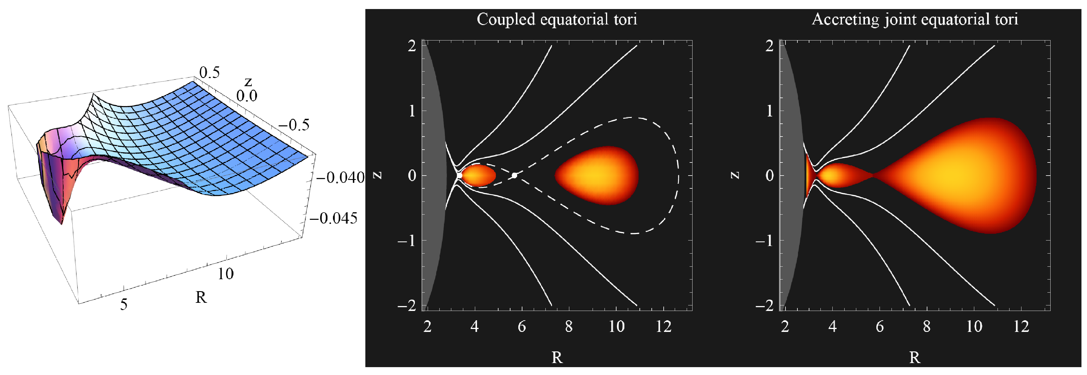
These toroidal structures appear, e.g., in the scenario of a dipole-like magnetic test field accompanying the Kerr (or non-rotating Schwarzschild, a = 0 ) black hole spacetime, where the fluid encircles the central object in the standard regime of uniform distribution of the specific angular momentum = const . The non-vanishing electromagnetic vector potential component reads [153]
A ϕ = - 3 8 M ( 2 + 2 r + r 2 ln r - 2 r ) sin 2 θ = - 3 8 M A ϕ ,
where A ϕ denotes the varying part of the vector potential; the constant dipole magnetic moment
M = 4 R 3 / 2 R - 2 1 / 2 6 ( R - 1 ) + 3 R ( R - 2 ) ln 1 - 2 R - 1 B ,
and B is the magnetic field strength measured at the characteristic radius R in the equatorial plane [154].
Considering the charge density transformation function in the form K = A ϕ , we reveal the following typical behavior of the potential W for different rotation regimes with constant specific angular momenta , and for the background magnetic dipole moments M .
  • For 5 . 15 and M = 2 . 6 , we get the potential W embodying two minima and two saddle points in the equatorial plane (corresponding to the positions of two equatorial centers, cusp and pseudo-cusp), allowing construction of either one equatorial torus, two coupled equatorial tori, or the construction of two coupled equatorial tori joint throw the pseudo-cusp and accreting onto the central compact object through the cusp (see Figure 21).
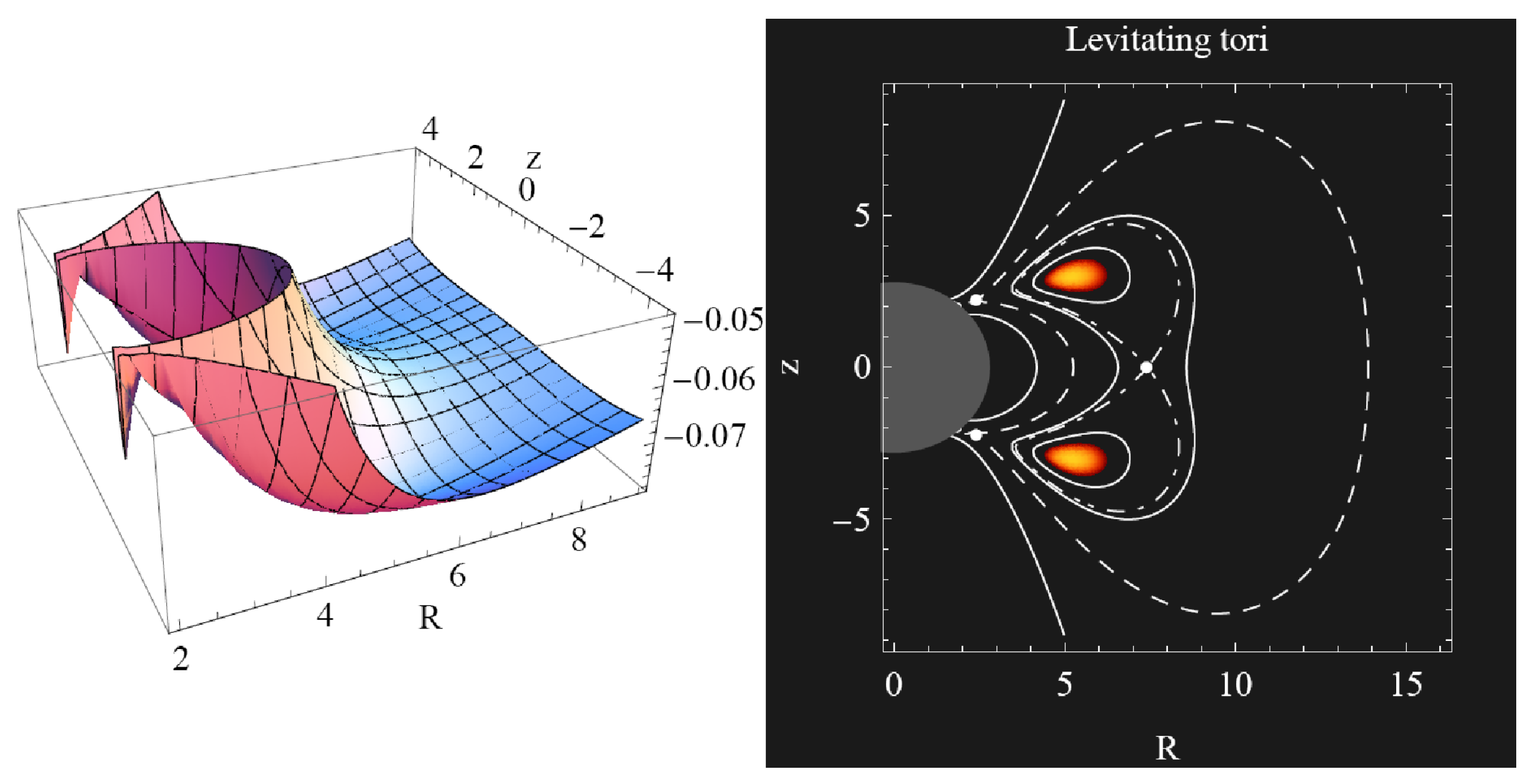
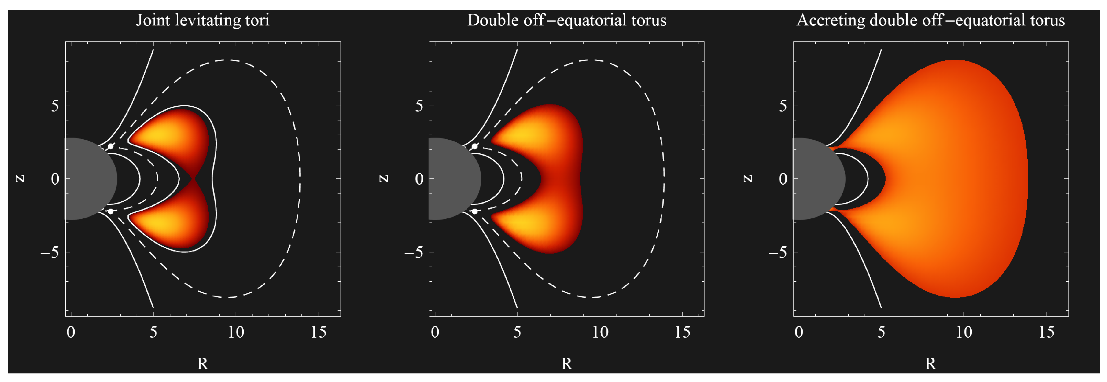
  • For 2 . 46 and M - 1 . 17 , we get the potential W embodying two minima and saddle points out of the equatorial plane, and one saddle point in the equatorial plane (corresponding to the positions of two off-equatorial centers and cusp, and to the equatorial pseudo-cusp), allowing construction of either two off-equatorial tori—the levitating tori, two levitating tori joint throw the pseudo-cusp, one double off-equatorial torus, or one double off-equatorial torus accreting onto the central compact object through the off-equatorial cusps (see Figure 22 and Figure 23).
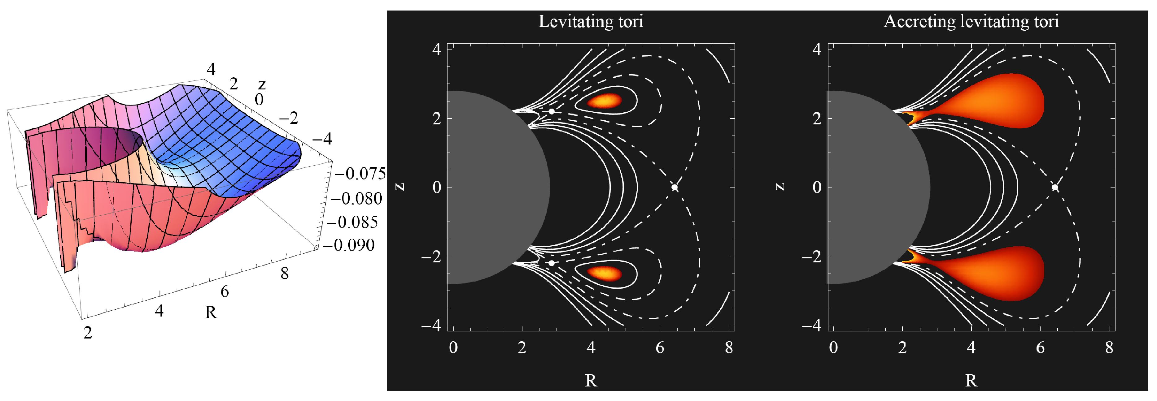
  • For 2 . 46 and M - 0 . 95 , we get the potential W embodying two minima and saddle points out of the equatorial plane, and one saddle point in the equatorial plane (corresponding to the positions of two off-equatorial centers and cusp, and to equatorial pseudo-cusp), allowing construction of either two levitating tori, or two levitating tori accreting onto the central compact object through the off-equatorial cusps (see Figure 24).

3.6.5.2. Polar Clouds

The cloud structures concentrated on the spacetime axis appear, e.g., in the scenario of asymptotically uniform magnetic test field (Wald test field) accompanying the Kerr spacetime that are described by the very well known and widely discussed Wald solution [23], where the fluid encircles the Kerr black hole in the rigid regime with uniform distribution of the angular velocity Ω = const . The behavior of the Kerr black hole immersed in the uniform magnetic field, with special focus on the electric charge induced on the black hole, has been discussed in detail in the previous subsection. Here, we assume that the non-vanishing electromagnetic vector potential components take the form [17,23]
A t = 1 2 B g t ϕ + 2 a g t t - 1 2 Q g t t - 1 2 Q ,
A ϕ = 1 2 B g ϕ ϕ + 2 a g t ϕ - 1 2 Q g t ϕ ,
where the parameter B corresponds to the strength of the magnetic field in infinity, and Q to the test charge of the central black hole.
Considering the charge density transformation function in the form K = k A , and rotation regime with the constant angular velocity profile Ω = - 1 . 6 × 10 - 3 , then, for the field parameters a = 0 . 9 , B = 6 . 5 × 10 - 5 and Q = 3 . 99 × 10 - 3 , we reveal the following typical behavior of the potential W.
  • For k = - 1 . 38 , we get the potential embodying two minima and saddle points on the polar axis, and two saddle points in the equatorial plane (corresponding to the positions of two polar centers and cusps, and equatorial pseudo-cusps), allowing construction of either two circling structures centered on the polar axis—the polar clouds, two polar clouds joint throw the pseudo-cusps, one closed encircling structure—the shell, or the accreting shell accreting onto the central black hole through the polar cusps (see Figure 25 and Figure 26). Note that the potential embodies also two equatorial maxima.
  • For k = - 1 . 3 , we get the potential embodying two minima and saddle points out on the polar axis, and two saddle points in the equatorial plane (corresponding to the positions of two polar centers and cusps, and equatorial pseudo-cusps), allowing construction of either two polar clouds, or two polar clouds accreting onto the central black hole through the polar cusps (see Figure 27). Note that the potential embodies also two equatorial maxima.

4. Conclusions

The combined influence of rotating black holes and cosmic repulsion, or external magnetic fields, is demonstrated by several very important phenomena related to accretion disks or tori.
The gravitational attraction of a black hole is balanced at the static radius r s = ( 3 M / Λ ) 1.3 by cosmic repulsion reflected by the relic cosmological constant. The static radius thus could give a natural limit on the extension of gravitationally bound systems in the universe accelerated by the relic cosmological constant [12]. Actually, extension of the accretion disks and tori orbiting rotating black holes is limited from above by the static radius, and for highly supermassive black holes with mass M 10 9 M , extension of the disks or tori restricted by the static radius is comparable to the extension of large galaxies containing such supermassive black holes in their center. The agreement of the extension of largest galaxies with the static radius related to their central supermassive black holes is complemented by the fact that the polytropic configurations representing galactic halos have extension restricted by the static radius determined by their gravitational mass and similar result holds for the largest known configurations, halos of galaxy clusters [15,66]. The relic cosmological constant thus limits extension of the gravitationally bound systems in the accelerated Universe.
There is an additional important role of the relic cosmological constant, related to flow of matter from accretion tori that occurs in close vicinity of the black hole along its rotation axis. The outflow of matter in highly energetic and collimated jets is strongly exceeding the extension of galaxy, determined by the static radius of the central supermassive black hole—the strong collimation of the open equipotential surfaces of the fluid that occurs while the surfaces are approaching and crossing the static radius can strongly support the collimation effect of the jets at distances overcoming the galaxy extension.
In contrast to the role of the cosmic repulsion that is most profound at large distances, near the static radius related to a given black hole, the external magnetic fields have the strongest role in the vicinity of the black holes due to the combined effect of the strong gravity, especially the frame dragging of the spacetime, and the magnetic field. There exists, in dependence on the character of the external magnetic field, a variety of non-conducting charged fluid toroidal structures; there are equatorial tori or double equatorial tori, but also off-equatorial tori or double off-equatorial tori, and orbiting charged clouds centered on the rotation axis. The Keplerian disks can have four states after ionization of the internal parts due to irradiation or other ionization processes—namely, the state of oscillatory motion, transition to the chaotic state corresponding to thick toroidal structure, destruction due to fall into the black hole, or escape to infinity along the magnetic field lines.
In the ionized Keplerian disks, the chaotic scattering process combined with the magnetic Penrose process can lead to creation of the UHECRs, i.e., protons and ions with energy reaching E = 10 22 eV. Such energies can be obtained by protons in the vicinity of the rotating black holes of mass M 10 10 M immersed in a magnetic field of strength B 10 5 G. For ions accelerated in the vicinity of the same black hole, the energy is lower by the factor given by the ratio of the specific charge of the proton and the considered ion. It is also shown that the maximal proton energy that can be reached, in the vicinity of SgrA*, where M 4 × 10 6 M and B 10 2 G, reads E 10 16 eV and corresponds to the knee of the observational data of registered UHECRs.
It can be shown that, during the motion in the vicinity of the black hole and the strong magnetic field, the radiation back reaction on the motion of protons and ions is negligible, so they are leaving the acceleration region with the energy ratio determined by the ratio of their specific charges. On the other hand, the radiation back reaction is relevant for the long travel from the source to the Earth in weak intergalactic fields, and it is different for protons and ions. Therefore, the ratio of the energies of protons and ions observed simultaneously at Earth can give relevant information on the distance of the source of the UHECRs. In the framework of the models of UHECR acceleration by the magnetic Penrose process, we thus have an important clue for search of the UHECRs sources.

Author Contributions

Z.S.: writing—original draft preparation and writing—review and editing; P.S.: Section 2.1 and Section 2.2; M.K.: Section 3.1Section 3.4; A.T.: Section 3.5; J.K.: Section 3.6. All authors have read and agreed to the published version of the manuscript.

Funding

Part of this work was funded by Czech Science Foundation grant No. 19-03950S

Acknowledgments

Authors would like to express their acknowledgement for the support of the Research Centre for Theoretical Physics and Astrophysics, Institute of Physics, Silesian University in Opava.

Conflicts of Interest

The authors declare no conflict of interest.

References

  1. Tchekhovskoy, A. Launching of Active Galactic Nuclei Jets. In The Formation and Disruption of Black Hole Jets; Contopoulos, I., Gabuzda, D., Kylafis, N., Eds.; Springer: Cham, Switzerland, 2015; Volume 414, pp. 45–82. [Google Scholar]
  2. Bardeen, J.M.; Petterson, J.A. The Lense-Thirring Effect and Accretion Disks around Kerr Black Holes. Astrophys. J. 1975, 195, L65. [Google Scholar] [CrossRef]
  3. Abramowicz, M.A.; Fragile, P.C. Foundations of Black Hole Accretion Disk Theory. Living Rev. Relat. 2013, 16, 1. [Google Scholar] [CrossRef] [Green Version]
  4. Novikov, I.D.; Thorne, K.S. Astrophysics of black holes. In Black Holes (Les Astres Occlus); Dewitt, C., Dewitt, B.S., Eds.; Gordon & Breach: New York, NY, USA, 1973; pp. 343–450. [Google Scholar]
  5. Kozlowski, M.; Jaroszynski, M.; Abramowicz, M.A. The analytic theory of fluid disks orbiting the Kerr black hole. Astron. Astrophys. 1978, 63, 209–220. [Google Scholar]
  6. Pugliese, D.; Stuchlík, Z. Ringed Accretion Disks: Equilibrium Configurations. Astrophys. J. Suppl. Ser. 2015, 221, 25. [Google Scholar] [CrossRef]
  7. Pugliese, D.; Stuchlík, Z. Ringed Accretion Disks: Instabilities. Astrophys. J. Suppl. Ser. 2016, 223, 27. [Google Scholar] [CrossRef] [Green Version]
  8. Pugliese, D.; Stuchlík, Z. Ringed Accretion Disks: Evolution of Double Toroidal Configurations. Astrophys. J. Suppl. Ser. 2017, 229, 40. [Google Scholar] [CrossRef] [Green Version]
  9. Stuchlík, Z. Influence of the RELICT Cosmological Constant on Accretion Discs. Mod. Phys. Lett. A 2005, 20, 561–575. [Google Scholar] [CrossRef]
  10. Stuchlík, Z.; Kološ, M.; Tursunov, A.A. Magnetized Black Holes: Ionized Keplerian Disks and Acceleration of Ultra-High Energy Particles. Proceedings 2019, 17, 13. [Google Scholar] [CrossRef] [Green Version]
  11. Stuchlik, Z. The Motion of Test Particles in Black-Hole Backgrounds with Non-Zero Cosmological Constant. Bull. Astron. Inst. Czechoslov. 1983, 34, 129–149. [Google Scholar]
  12. Stuchlík, Z.; Hledík, S. Some properties of the Schwarzschild-de Sitter and Schwarzschild-anti-de Sitter spacetimes. Phys. Rev. D 1999, 60, 044006. [Google Scholar] [CrossRef]
  13. Stuchlík, Z.; Slaný, P. Equatorial circular orbits in the Kerr–de Sitter spacetimes. Phys. Rev. D 2004, 69, 064001. [Google Scholar] [CrossRef] [Green Version]
  14. Slaný, P.; Stuchlík, Z. Relativistic thick discs in the Kerr–de Sitter backgrounds. Class. Quantum Gravity 2005, 22, 3623–3651. [Google Scholar] [CrossRef]
  15. Stuchlík, Z.; Hledík, S.; Novotný, J. General relativistic polytropes with a repulsive cosmological constant. Phys. Rev. D 2016, 94, 103513. [Google Scholar] [CrossRef] [Green Version]
  16. Stuchlík, Z.; Slaný, P.; Hledík, S. Equilibrium configurations of perfect fluid orbiting Schwarzschild-de Sitter black holes. Astron. Astrophys. 2000, 363, 425–439. [Google Scholar]
  17. Kovář, J.; Kopáček, O.; Karas, V.; Stuchlík, Z. Off-equatorial orbits in strong gravitational fields near compact objects—II: Halo motion around magnetic compact stars and magnetized black holes. Class. Quantum Gravity 2010, 27, 135006. [Google Scholar] [CrossRef]
  18. Kovář, J.; Slaný, P.; Cremaschini, C.; Stuchlík, Z.; Karas, V.; Trova, A. Charged perfect fluid tori in strong central gravitational and dipolar magnetic fields. Phys. Rev. D 2016, 93, 124055. [Google Scholar] [CrossRef]
  19. Kovář, J.; Slaný, P.; Cremaschini, C.; Stuchlík, Z.; Karas, V.; Trova, A. Electrically charged matter in rigid rotation around magnetized black hole. Phys. Rev. D 2014, 90, 044029. [Google Scholar] [CrossRef] [Green Version]
  20. Frolov, V.P.; Shoom, A.A. Motion of charged particles near a weakly magnetized Schwarzschild black hole. Phys. Rev. D 2010, 82, 084034. [Google Scholar] [CrossRef] [Green Version]
  21. Kovář, J.; Stuchlík, Z.; Karas, V. Off-equatorial orbits in strong gravitational fields near compact objects. Class. Quantum Gravity 2008, 25, 095011. [Google Scholar] [CrossRef] [Green Version]
  22. Kološ, M.; Tursunov, A.; Stuchlík, Z. Possible signature of the magnetic fields related to quasi-periodic oscillations observed in microquasars. Eur. Phys. J. C 2017, 77, 860. [Google Scholar] [CrossRef]
  23. Wald, R.M. Black hole in a uniform magnetic field. Phys. Rev. D 1974, 10, 1680–1685. [Google Scholar] [CrossRef]
  24. Prasanna, A.R. General-relativistic analysis of charged-particle motion in electromagnetic fields surrounding black holes. Nuovo Cimento Rivista Serie 1980, 3, 1–53. [Google Scholar] [CrossRef]
  25. Aliev, A.N.; Galtsov, D.V. Radiation from relativistic particles in nongeodesic motion in a strong gravitational field. Gen. Relat. Gravit. 1981, 13, 899–912. [Google Scholar] [CrossRef]
  26. Kopáček, O.; Karas, V.; Kovář, J.; Stuchlík, Z. Transition from Regular to Chaotic Circulation in Magnetized Coronae near Compact Objects. Astrophys. J. 2010, 722, 1240–1259. [Google Scholar] [CrossRef]
  27. Abdujabbarov, A.A.; Ahmedov, B.J.; Jurayeva, N.B. Charged-particle motion around a rotating non-Kerr black hole immersed in a uniform magnetic field. Phys. Rev. D 2013, 87, 064042. [Google Scholar] [CrossRef]
  28. Al Zahrani, A.M.; Frolov, V.P.; Shoom, A.A. Critical escape velocity for a charged particle moving around a weakly magnetized Schwarzschild black hole. Phys. Rev. D 2013, 87, 084043. [Google Scholar] [CrossRef] [Green Version]
  29. Kopáček, O.; Karas, V. Inducing Chaos by Breaking Axial Symmetry in a Black Hole Magnetosphere. Astrophys. J. 2014, 787, 117. [Google Scholar] [CrossRef] [Green Version]
  30. Shiose, R.; Kimura, M.; Chiba, T. Motion of charged particles around a weakly magnetized rotating black hole. Phys. Rev. D 2014, 90, 124016. [Google Scholar] [CrossRef] [Green Version]
  31. Kološ, M.; Stuchlík, Z.; Tursunov, A. Quasi-harmonic oscillatory motion of charged particles around a Schwarzschild black hole immersed in a uniform magnetic field. Class. Quantum Gravity 2015, 32, 165009. [Google Scholar] [CrossRef] [Green Version]
  32. Tursunov, A.; Stuchlík, Z.; Kološ, M. Circular orbits and related quasi-harmonic oscillatory motion of charged particles around weakly magnetized rotating black holes. Phys. Rev. D 2016, 93, 084012. [Google Scholar] [CrossRef] [Green Version]
  33. Stuchlík, Z.; Kološ, M. Acceleration of the charged particles due to chaotic scattering in the combined black hole gravitational field and asymptotically uniform magnetic field. Eur. Phys. J. C 2016, 76, 32. [Google Scholar] [CrossRef] [Green Version]
  34. Kopáček, O.; Karas, V. Near-horizon Structure of Escape Zones of Electrically Charged Particles around Weakly Magnetized Rotating Black Hole. Astrophys. J. 2018, 853, 53. [Google Scholar] [CrossRef] [Green Version]
  35. Pánis, R.; Kološ, M.; Stuchlík, Z. Determination of chaotic behaviour in time series generated by charged particle motion around magnetized Schwarzschild black holes. arXiv 2019, arXiv:1905.01186. [Google Scholar] [CrossRef] [Green Version]
  36. Tursunov, A.; Kološ, M.; Stuchlík, Z.; Galtsov, D.V. Radiation Reaction of Charged Particles Orbiting a Magnetized Schwarzschild Black Hole. Astrophys. J. 2018, 861, 2. [Google Scholar] [CrossRef]
  37. Tursunov, A.A.; Kološ, M.; Stuchlík, Z. Orbital widening due to radiation reaction around a magnetized black hole. Astronomische Nachrichten 2018, 339, 341–346. [Google Scholar] [CrossRef] [Green Version]
  38. Dadhich, N.; Tursunov, A.; Ahmedov, B.; Stuchlík, Z. The distinguishing signature of magnetic Penrose process. Mon. Not. R. Astron. Soc. 2018, 478, L89–L94. [Google Scholar] [CrossRef] [Green Version]
  39. Tursunov, A.A.; Stuchlík, Z.; Kološ, M.; Dadhich, N.; Ahmedov, B. Supermassive Black Hole as a source of Ultra-High-Energy Cosmic Rays. arXiv 2019, arXiv:1811.11216v1. [Google Scholar]
  40. Abramowicz, M.; Jaroszynski, M.; Sikora, M. Relativistic, accreting disks. Astron. Astrophys. 1978, 63, 221–224. [Google Scholar]
  41. Komissarov, S.S. Magnetized tori around Kerr black holes: analytic solutions with a toroidal magnetic field. Mon. Not. R. Astron. Soc. 2006, 368, 993–1000. [Google Scholar] [CrossRef]
  42. Blandford, R.D.; Znajek, R.L. Electromagnetic extraction of energy from Kerr black holes. Mon. Not. R. Astron. Soc. 1977, 179, 433–456. [Google Scholar] [CrossRef]
  43. Kovář, J.; Slaný, P.; Stuchlík, Z.; Karas, V.; Cremaschini, C.; Miller, J.C. Role of electric charge in shaping equilibrium configurations of fluid tori encircling black holes. Phys. Rev. D 2011, 84, 084002. [Google Scholar] [CrossRef] [Green Version]
  44. Riess, A.G.; Filippenko, A.V.; Challis, P.; Clocchiatti, A.; Diercks, A.; Garnavich, P.M.; Gilliland, R.L.; Hogan, C.J.; Jha, S.; Kirshner, R.P.; et al. Observational Evidence from Supernovae for an Accelerating Universe and a Cosmological Constant. Astronom. J. 1998, 116, 1009–1038. [Google Scholar] [CrossRef] [Green Version]
  45. Wang, M.L.D.L.W. Dark energy: A brief review. Front. Phys. 2013, 8, 828–846. [Google Scholar]
  46. Bardeen, J.M.; Press, W.H.; Teukolsky, S.A. Rotating Black Holes: Locally Nonrotating Frames, Energy Extraction, and Scalar Synchrotron Radiation. Astrophys. J. 1972, 178, 347–370. [Google Scholar] [CrossRef]
  47. Stuchlík, Z. Equatorial circular orbits and the motion of the shell of dust in the field of a rotating naked singularity. Bull. Astron. Inst. Czechoslov. 1980, 31, 129–144. [Google Scholar]
  48. Stuchlík, Z.; Hledík, S.; Truparová, K. Evolution of Kerr superspinars due to accretion counterrotating thin discs. Class. Quantum Gravity 2011, 28, 155017. [Google Scholar] [CrossRef]
  49. Stuchlík, Z.; Kotrlová, A. Orbital resonances in discs around braneworld Kerr black holes. Gen. Relat. Gravit. 2009, 41, 1305–1343. [Google Scholar] [CrossRef] [Green Version]
  50. Blaschke, M.; Stuchlík, Z. Efficiency of the Keplerian accretion in braneworld Kerr-Newman spacetimes and mining instability of some naked singularity spacetimes. Phys. Rev. D 2016, 94, 086006. [Google Scholar] [CrossRef] [Green Version]
  51. Stuchlík, Z.; Hledík, S. Equilibrium of a charged spinning test particle in Reissner-Nordström backgrounds with a nonzero cosmological constant. Phys. Rev. D 2001, 64, 104016. [Google Scholar] [CrossRef]
  52. Carter, B. Black hole equilibrium states. In Black Holes (Les Astres Occlus); Dewitt, C., Dewitt, B.S., Eds.; Gordon & Breach: New York, NY, USA, 1973; pp. 57–214. [Google Scholar]
  53. Gimon, E.G.; Hořava, P. Astrophysical violations of the Kerr bound as a possible signature of string theory. Phys. Lett. B 2009, 672, 299–302. [Google Scholar] [CrossRef] [Green Version]
  54. Stuchlík, Z.; Schee, J. Appearance of Keplerian discs orbiting Kerr superspinars. Class. Quantum Gravity 2010, 27, 215017. [Google Scholar] [CrossRef] [Green Version]
  55. Stuchlík, Z.; Schee, J. Observational phenomena related to primordial Kerr superspinars. Class. Quantum Gravity 2012, 29, 065002. [Google Scholar] [CrossRef]
  56. Stuchlík, Z.; Schee, J. Ultra-high-energy collisions in the superspinning Kerr geometry. Class. Quantum Gravity 2013, 30, 075012. [Google Scholar] [CrossRef]
  57. Akcay, S.; Matzner, R.A. The Kerr-de Sitter universe. Class. Quantum Gravity 2011, 28, 085012. [Google Scholar] [CrossRef] [Green Version]
  58. Brill, D.; Hayward, S.A. Global structure of a black hole cosmos and its extremes. Class. Quantum Gravity 1994, 11, 359–370. [Google Scholar] [CrossRef] [Green Version]
  59. Hayward, S.A.; Shiromizu, T.; Nakao, K.-i. A cosmological constant limits the size of black holes. Phys. Rev. D 1994, 49, 5080–5085. [Google Scholar] [CrossRef] [Green Version]
  60. Bicak, J.; Stuchlik, Z. On the latitudinal and radial motion in the field of a rotating black hole. Bull. Astron. Inst. Czechoslov. 1976, 27, 129–133. [Google Scholar]
  61. Misner, C.W.; Thorne, K.S.; Wheeler, J.A. Gravitation; W. H. Freeman: Princeton, NJ, USA, 1973. [Google Scholar]
  62. Balek, V.; Bicak, J.; Stuchlik, Z. The Motion of the Charged Particles in the Field of Rotating Charged Black Holes and Naked Singularities. II. The Motion in the Equatorial Plane. Bull. Astron. Inst. Czechoslov. 1989, 40, 133. [Google Scholar]
  63. Page, D.N.; Thorne, K.S. Disk-Accretion onto a Black Hole. Time-Averaged Structure of Accretion Disk. Astrophys. J. 1974, 191, 499–506. [Google Scholar] [CrossRef]
  64. Chandrasekhar, S. The mathematical theory of black holes. In Proceedings of the General Relativity and Gravitation Conference, Padua, Italy, 4–9 July 1984; pp. 5–26. [Google Scholar]
  65. Stuchlík, Z.; Schee, J. Influence of the cosmological constant on the motion of Magellanic Clouds in the gravitational field of Milky Way. J. Cosmol. Astropart. Phys. 2011, 9, 18. [Google Scholar] [CrossRef]
  66. Stuchlík, Z.; Schee, J.; Toshmatov, B.; Hladík, J.; Novotný, J. Gravitational instability of polytropic spheres containing region of trapped null geodesics: A possible explanation of central supermassive black holes in galactic halos. J. Cosmol. Astropart. Phys. 2017, 2017, 056. [Google Scholar] [CrossRef]
  67. Stuchlík, Z.; Hledík, S. Equatorial photon motion in the Kerr-Newman spacetimes with a non-zero cosmological constant. Class. Quantum Gravity 2000, 17, 4541–4576. [Google Scholar] [CrossRef] [Green Version]
  68. Charbulák, D.; Stuchlík, Z. Photon motion in Kerr-de Sitter spacetimes. Eur. Phys. J. C 2017, 77, 897. [Google Scholar] [CrossRef]
  69. Stuchlík, Z.; Charbulák, D.; Schee, J. Light escape cones in local reference frames of Kerr-de Sitter black hole spacetimes and related black hole shadows. Eur. Phys. J. C 2018, 78, 180. [Google Scholar] [CrossRef] [Green Version]
  70. Boyer, R.H. Rotating fluid masses in general relativity. Proc. Camb. Philos. Soc. 1965, 61, 527. [Google Scholar] [CrossRef]
  71. Stuchlík, Z.; Slaný, P.; Kovář, J. Pseudo-Newtonian and general relativistic barotropic tori in Schwarzschild-de Sitter spacetimes. Class. Quantum Gravity 2009, 26, 215013. [Google Scholar] [CrossRef] [Green Version]
  72. Seguin, F.H. The stability of nonuniform rotation in relativistic stars. Astrophys. J. 1975, 197, 745. [Google Scholar] [CrossRef]
  73. Abramowicz, M.A.; Calvani, M.; Nobili, L. Thick accretion disks with super-Eddington luminosities. Astrophys. J. 1980, 242, 772–788. [Google Scholar] [CrossRef]
  74. Spergel, D.N.; Verde, L.; Peiris, H.V.; Komatsu, E.; Nolta, M.R.; Bennett, C.L.; Halpern, M.; Hinshaw, G.; Jarosik, N.; Kogut, A.; et al. First Year Wilkinson Microwave Anisotropy Probe (WMAP) Observations: Determination of Cosmological Parameters. Astrophys. J. Suppl. 2003, 148, 175. [Google Scholar] [CrossRef] [Green Version]
  75. Ostlie, B.W.C.A. An Introduction to Modern Astrophysics; Addison-Wesley: Reading, MA, USA, 1996. [Google Scholar]
  76. Zanotti, L.R. Dynamics of thick discs around Schwarzschild-de Sitter black holes. Astron. Astrophys. 2003, 412, 603. [Google Scholar]
  77. Raine, J.F.K. Accretion Power in Astrophysics, 3rd ed.; Cambridge University Press: Cambridge, UK, 2002. [Google Scholar]
  78. Ruffini, R. On the energetics of black holes. In Black Holes (Les Astres Occlus); Dewitt, C., Dewitt, B.S., Eds.; Gordon & Breach: New York, NY, USA, 1973; pp. 451–546. [Google Scholar]
  79. Balbus, S.A.; Hawley, J.F. A powerful local shear instability in weakly magnetized disks. I - Linear analysis. II—Nonlinear evolution. Astrophys. J. 1991, 376, 214–233. [Google Scholar] [CrossRef]
  80. Penrose, R. Gravitational Collapse:The Role of General Relativity. Nuovo Cimento Rivista Serie 1969, 1, 252. [Google Scholar]
  81. Tursunov, A.; Dadhich, N. Fifty Years of Energy Extraction from Rotating Black Hole: Revisiting Magnetic Penrose Process. Universe 2019, 5, 125. [Google Scholar] [CrossRef] [Green Version]
  82. Trova, A.; Schroven, K.; Hackmann, E.; Karas, V.; Kovář, J.; Slaný, P. Equilibrium configurations of charged fluid around Kerr black hole. Phys. Rev. D 2018, 97, 104019. [Google Scholar] [CrossRef] [Green Version]
  83. Slaný, P.; Kovář, J.; Stuchlík, Z.; Karas, V. Charged Tori in Spherical Gravitational and Dipolar Magnetic Fields. Astrophys. J. Suppl. 2013, 205, 3. [Google Scholar] [CrossRef]
  84. Dovčiak, M.; Muleri, F.; Goosmann, R.W.; Karas, V.; Matt, G. Polarization in lamp-post model of black-hole accretion discs. J. Phys. Conf. Ser. 2012, 372, 012056. [Google Scholar] [CrossRef] [Green Version]
  85. Petterson, J.A. Magnetic field of a current loop around a Schwarzschild black hole. Phys. Rev. D 1974, 10, 3166–3170. [Google Scholar] [CrossRef]
  86. Eatough, R.P.; Falcke, H.; Karuppusamy, R.; Lee, K.J.; Champion, D.J.; Keane, E.F.; Desvignes, G.; Schnitzeler, D.H.F.M.; Spitler, L.G.; Kramer, M.; et al. A strong magnetic field around the supermassive black hole at the centre of the Galaxy. Nature 2013, 501, 391–394. [Google Scholar] [CrossRef] [PubMed] [Green Version]
  87. Doeleman, S.S.; Fish, V.L.; Schenck, D.E.; Beaudoin, C.; Blundell, R.; Bower, G.C.; Broderick, A.E.; Chamberlin, R.; Freund, R.; Friberg, P.; et al. Jet-Launching Structure Resolved Near the Supermassive Black Hole in M87. Science 2012, 338, 355. [Google Scholar] [CrossRef] [Green Version]
  88. Daly, R.A. Black Hole Spin and Accretion Disk Magnetic Field Strength Estimates for More Than 750 Active Galactic Nuclei and Multiple Galactic Black Holes. Astrophys. J. 2019, 886, 37. [Google Scholar] [CrossRef]
  89. Gal’tsov, D.V.; Petukhov, V.I. Black hole in an external magnetic field. Sov. J. Exp. Theor. Phys. 1978, 47, 419. [Google Scholar]
  90. Bicak, J.; Stuchlik, Z. The fall of the shell of dust on to a rotating black hole. Mon. Not. R. Astron. Soc. 1976, 175, 381–393. [Google Scholar] [CrossRef]
  91. Bicak, J.; Janis, V. Magnetic fluxes across black holes. Mon. Not. R. Astron. Soc. 1985, 212, 899–915. [Google Scholar] [CrossRef] [Green Version]
  92. Zajaček, M.; Tursunov, A.; Eckart, A.; Britzen, S. On the charge of the Galactic centre black hole. Mon. Not. R. Astron. Soc. 2018, 480, 4408–4423. [Google Scholar] [CrossRef]
  93. Bičák, J.; Ledvinka, T. Electromagnetic fields around black holes and Meissner effect. Nuovo Cimento B Serie 2000, 115, 739. [Google Scholar]
  94. Komissarov, S.S. Blandford-Znajek Mechanism versus Penrose Process. J. Korean Phys. Soc. 2009, 54, 2503. [Google Scholar] [CrossRef] [Green Version]
  95. Punsly, B. Black Hole Gravitohydromagnetics; Springer: Heidelberg, Germany, 2001. [Google Scholar]
  96. Komissarov, S.S. Electrodynamics of black hole magnetospheres. Mon. Not. R. Astron. Soc. 2004, 350, 427–448. [Google Scholar] [CrossRef] [Green Version]
  97. Nakamura, M.; Asada, K.; Hada, K.; Pu, H.Y.; Noble, S.; Tseng, C.; Toma, K.; Kino, M.; Nagai, H.; Takahashi, K.; et al. Parabolic Jets from the Spinning Black Hole in M87. Astrophys. J. 2018, 868, 146. [Google Scholar] [CrossRef] [Green Version]
  98. Kopáček, O.; Karas, V.; Kovář, J.; Stuchlík, Z. Application of a symplectic integrator in a non-integrable relativistic system. In RAGtime 10-13: Workshops on Black Holes and Neutron Stars; Stuchlík, Z., Török, G., Pecháček, T., Eds.; Silesian University: Opava, Czech Republic, 2014; pp. 123–132. [Google Scholar]
  99. Bičák, J.; Stuchlík, Z.; Balek, V. The motion of charged particles in the field of rotating charged black holes and naked singularities. Bull. Astron. Inst. Czechoslov. 1989, 40, 65–92. [Google Scholar]
  100. Stuchlík, Z.; Kološ, M. String loops in the field of braneworld spherically symmetric black holes and naked singularities. J. Cosmol. Astropart. Phys. 2012, 10, 008. [Google Scholar] [CrossRef]
  101. Stuchlík, Z.; Kološ, M. String loops oscillating in the field of Kerr black holes as a possible explanation of twin high-frequency quasiperiodic oscillations observed in microquasars. Phys. Rev. D 2014, 89, 065007. [Google Scholar] [CrossRef] [Green Version]
  102. Remillard, R.A.; McClintock, J.E. X-Ray Properties of Black-Hole Binaries. Annu. Rev. Astron. Astrophys. 2006, 44, 49–92. [Google Scholar] [CrossRef] [Green Version]
  103. Carpano, S.; Jin, C. Discovery of a 23.8 h QPO in the Swift light curve of XMMU J134736.6+173403. Mon. Not. R. Astron. Soc. 2018, 477, 3178–3184. [Google Scholar] [CrossRef] [Green Version]
  104. Stuchlík, Z.; Kotrlová, A.; Török, G. Multi-resonance orbital model of high-frequency quasi-periodic oscillations: possible high-precision determination of black hole and neutron star spin. Astron. Astrophys. 2013, 552, A10. [Google Scholar] [CrossRef] [Green Version]
  105. Török, G.; Stuchlík, Z. Radial and vertical epicyclic frequencies of Keplerian motion in the field of Kerr naked singularities. Comparison with the black hole case and possible instability of naked-singularity accretion discs. Astron. Astrophys. 2005, 437, 775–788. [Google Scholar] [CrossRef]
  106. Cremaschini, C.; Stuchlík, Z. Magnetic loop generation by collisionless gravitationally bound plasmas in axisymmetric tori. Phys. Rev. E 2013, 87, 043113. [Google Scholar] [CrossRef]
  107. Belloni, T.M.; Sanna, A.; Méndez, M. High-frequency quasi-periodic oscillations in black hole binaries. Mon. Not. R. Astron. Soc. 2012, 426, 1701–1709. [Google Scholar] [CrossRef] [Green Version]
  108. Abramowicz, M.A.; Kluźniak, W. A precise determination of black hole spin in GRO J1655-40. Astron. Astrophys. 2001, 374, L19–L20. [Google Scholar] [CrossRef] [Green Version]
  109. Török, G.; Abramowicz, M.A.; Kluźniak, W.; Stuchlík, Z. The orbital resonance model for twin peak kHz quasi periodic oscillations in microquasars. Astron. Astrophys. 2005, 436, 1–8. [Google Scholar] [CrossRef]
  110. Goluchová, K.; Török, G.; Šrámková, E.; Abramowicz, M.A.; Stuchlík, Z.; Horák, J. Mass of the active galactic nucleus black hole XMMUJ134736.6+173403. Astron. Astrophys. 2019, 622, L8. [Google Scholar] [CrossRef]
  111. Török, G.; Kotrlová, A.; Šrámková, E.; Stuchlík, Z. Confronting the models of 3:2 quasiperiodic oscillations with the rapid spin of the microquasar GRS 1915+105. Astron. Astrophys. 2011, 531, A59. [Google Scholar] [CrossRef] [Green Version]
  112. Stuchlík, Z.; Kološ, M. Models of quasi-periodic oscillations related to mass and spin of the GRO J1655-40 black hole. Astron. Astrophys. 2016, 586, A130. [Google Scholar] [CrossRef] [Green Version]
  113. McClintock, J.E.; Narayan, R.; Davis, S.W.; Gou, L.; Kulkarni, A.; Orosz, J.A.; Penna, R.F.; Remillard, R.A.; Steiner, J.F. Measuring the spins of accreting black holes. Class. Quantum Gravity 2011, 28, 114009. [Google Scholar] [CrossRef] [Green Version]
  114. Stuchlík, Z.; Kološ, M. Mass of intermediate black hole in the source M82 X-1 restricted by models of twin high-frequency quasi-periodic oscillations. Mon. Not. R. Astron. Soc. 2015, 451, 2575–2588. [Google Scholar] [CrossRef] [Green Version]
  115. Stella, L.; Vietri, M. Lense-Thirring Precession and Quasi-periodic Oscillations in Low-Mass X-Ray Binaries. Astrophys. J. Lett. 1998, 492, L59. [Google Scholar] [CrossRef]
  116. Parthasarathy, S.; Wagh, S.M.; Dhurandhar, S.V.; Dadhich, N. High efficiency of the Penrose process of energy extraction from rotating black holes immersed in electromagnetic fields. Astrophys. J. 1986, 307, 38–46. [Google Scholar] [CrossRef]
  117. Shakura, N.I. Geodesics in a Kerr Metric. Sov. Astron. Lett. 1987, 13, 99. [Google Scholar]
  118. de Felice, F.; Calvani, M. Orbital and vortical motion in the Kerr metric. Nuovo Cimento B Serie 1972, 10, 447–458. [Google Scholar]
  119. Dhurandhar, S.V.; Dadhich, N. Energy-extraction processes from a Kerr black hole immersed in a magnetic field. II. The formalism. Phys. Rev. D 1984, 30, 1625–1631. [Google Scholar] [CrossRef]
  120. Bardeen, J.M. Timelike and null geodesics in the Kerr metric. In Black Holes (Les Astres Occlus); Gordon & Breach: New York, NY, USA, 1973; pp. 215–239. [Google Scholar]
  121. Blandford, R.D.; Payne, D.G. Hydromagnetic flows from accretion disks and the production of radio jets. Mon. Not. R. Astron. Soc. 1982, 199, 883–903. [Google Scholar] [CrossRef] [Green Version]
  122. Greisen, K. End to the Cosmic-Ray Spectrum? Phys. Rev. Lett. 1966, 16, 748–750. [Google Scholar] [CrossRef]
  123. Parsa, M.; Eckart, A.; Shahzamanian, B.; Karas, V.; Zajaček, M.; Zensus, J.A.; Straubmeier, C. Investigating the Relativistic Motion of the Stars Near the Supermassive Black Hole in the Galactic Center. Astrophys. J. 2017, 845, 22. [Google Scholar] [CrossRef] [Green Version]
  124. Eckart, A.; Schödel, R.; Meyer, L.; Trippe, S.; Ott, T.; Genzel, R. Polarimetry of near-infrared flares from Sagittarius A*. Astron. Astrophys. 2006, 455, 1–10. [Google Scholar] [CrossRef]
  125. Eckart, A.; Hüttemann, A.; Kiefer, C.; Britzen, S.; Zajaček, M.; Lämmerzahl, C.; Stöckler, M.; Valencia-S, M.; Karas, V.; García-Marín, M. The Milky Way’s Supermassive Black Hole: How Good a Case Is It? Found. Phys. 2017, 47, 553–624. [Google Scholar] [CrossRef] [Green Version]
  126. Bonazzola, S.; Gourgoulhon, E.; Marck, J.A. Numerical approach for high precision 3D relativistic star models. Phys. Rev. D 1998, 58, 104020. [Google Scholar] [CrossRef] [Green Version]
  127. Gourgoulhon, E.; Grandclément, P.; Marck, J.A.; Novak, J.; Taniguchi, K. LORENE: Spectral methods differential equations solver. arXiv 2016, arXiv:1608.018. [Google Scholar]
  128. Hartle, J.B.; Thorne, K.S. Slowly Rotating Relativistic Stars. II. Models for Neutron Stars and Supermassive Stars. Astrophys. J. 1968, 153, 807. [Google Scholar] [CrossRef]
  129. Török, G.; Bakala, P.; Šrámková, E.; Stuchlík, Z.; Urbanec, M. On Mass Constraints Implied by the Relativistic Precession Model of Twin-peak Quasi-periodic Oscillations in Circinus X-1. Astrophys. J. 2010, 714, 748–757. [Google Scholar] [CrossRef] [Green Version]
  130. Urbanec, M.; Miller, J.C.; Stuchlík, Z. Quadrupole moments of rotating neutron stars and strange stars. Mon. Not. R. Astron. Soc. 2013, 433, 1903–1909. [Google Scholar] [CrossRef] [Green Version]
  131. Urbancová, G.; Urbanec, M.; Török, G.; Stuchlík, Z.; Blaschke, M.; Miller, J.C. Epicyclic Oscillations in the Hartle-Thorne External Geometry. Astrophys. J. 2019, 877, 66. [Google Scholar] [CrossRef] [Green Version]
  132. Stuchlík, Z.; Kološ, M. Test of the string loop oscillation model using kHz quasiperiodic oscillations in a neutron star binary. Gen. Relat. Gravit. 2015, 47, 27. [Google Scholar] [CrossRef] [Green Version]
  133. Landau, L.D.; Lifshitz, E.M. The Classical Theory of Fields; Pergamon Press: Oxford, UK, 1976. [Google Scholar]
  134. Poisson, E. The Motion of Point Particles in Curved Spacetime. Living Rev. Relat. 2004, 7, 6. [Google Scholar] [CrossRef] [Green Version]
  135. DeWitt, B.S.; Brehme, R.W. Radiation damping in a gravitational field. Ann. Phys. 1960, 9, 220–259. [Google Scholar] [CrossRef]
  136. Hobbs, J. A vierbein formalism of radiation damping. Ann. Phys. 1968, 47, 141–165. [Google Scholar] [CrossRef]
  137. Dewitt, B.S.; Dewitt, C.M. Falling charges. Phys. N. Y. 1964, 1, 3–20. [Google Scholar] [CrossRef] [Green Version]
  138. Smith, A.G.; Will, C.M. Force on a static charge outside a Schwarzschild black hole. Phys. Rev. D 1980, 22, 1276–1284. [Google Scholar] [CrossRef]
  139. Chrzanowski, P.L.; Misner, C.W. Geodesic synchrotron radiation in the Kerr geometry by the method of asymptotically factorized Green’s functions. Phys. Rev. D 1974, 10, 1701–1721. [Google Scholar] [CrossRef]
  140. Gal’tsov, D.V. Radiation reaction in the Kerr gravitational field. J. Phys. A Math. Gen. 1982, 15, 3737–3749. [Google Scholar] [CrossRef]
  141. Sokolov, A.A.; Ternov, I.M.; Aliev, A.N.; Gal’tsov, D.V. Synchrotron radiation in curved space-time. Sov. Phys. J. 1983, 26, 36–40. [Google Scholar] [CrossRef]
  142. Sokolov, A.A.; Gal’tsov, D.V.; Petukhov, V.I. Radiation emitted by relativistic particles moving in the vicinity of the Schwarzschild black hole, immersed in an external magnetic field. Phys. Lett. A 1978, 68, 1–2. [Google Scholar] [CrossRef]
  143. Shoom, A.A. Synchrotron radiation from a weakly magnetized Schwarzschild black hole. Phys. Rev. D 2015, 92, 124066. [Google Scholar] [CrossRef] [Green Version]
  144. Piotrovich, M.Y.; Silant’ev, N.A.; Gnedin, Y.N.; Natsvlishvili, T.M. Magnetic fields and quasi-periodic oscillations of black hole radiation. Astrophys. Bull. 2011, 66, 320–324. [Google Scholar] [CrossRef]
  145. Baczko, A.K.; Schulz, R.; Kadler, M.; Ros, E.; Perucho, M.; Krichbaum, T.P.; Böck, M.; Bremer, M.; Grossberger, C.; Lindqvist, M.; et al. A highly magnetized twin-jet base pinpoints a supermassive black hole. Astron. Astrophys. 2016, 593, A47. [Google Scholar] [CrossRef] [Green Version]
  146. Johnson, M.D.; Fish, V.L.; Doeleman, S.S.; Marrone, D.P.; Plambeck, R.L.; Wardle, J.F.C.; Akiyama, K.; Asada, K.; Beaudoin, C.; Blackburn, L.; et al. Resolved magnetic-field structure and variability near the event horizon of Sagittarius A*. Science 2015, 350, 1242–1245. [Google Scholar] [CrossRef] [PubMed] [Green Version]
  147. Kovář, J. Spiral motion formation in astrophysics. Eur. Phys. J. Plus 2013, 128, 142. [Google Scholar] [CrossRef]
  148. Kovář, J.; Kopáček, O.; Karas, V.; Kojima, Y. Regular and chaotic orbits near a massive magnetic dipole. Class. Quantum Gravity 2013, 30, 025010. [Google Scholar] [CrossRef] [Green Version]
  149. Pugliese, D.; Stuchlík, Z. Relating Kerr SMBHs in active galactic nuclei to RADs configurations. Class. Quantum Gravity 2018, 35, 185008. [Google Scholar] [CrossRef] [Green Version]
  150. Pugliese, D.; Stuchlík, Z. RADs energetics and constraints on emerging tori collisions around super-massive Kerr black holes. Eur. Phys. J. C 2019, 79, 288. [Google Scholar] [CrossRef]
  151. Cremaschini, C.; Kovář, J.; Slaný, P.; Stuchlík, Z.; Karas, V. Kinetic Theory of Equilibrium Axisymmetric Collisionless Plasmas in Off-equatorial Tori around Compact Objects. Astrophys. J. Suppl. 2013, 209, 15. [Google Scholar] [CrossRef] [Green Version]
  152. Bao, G.; Stuchlik, Z. Accretion Disk Self-Eclipse: X-Ray Light Curve and Emission Line. Astrophys. J. 1992, 400, 163. [Google Scholar] [CrossRef]
  153. Prasanna, A.R.; Sengupta, S. Charged particle trajectories in the presence of a toroidal magnetic field on a Schwarzschild background. Phys. Lett. A 1994, 193, 25. [Google Scholar] [CrossRef]
  154. Bakala, P.; Šrámková, E.; Stuchlík, Z.; Török, G. On magnetic-field-induced non-geodesic corrections to relativistic orbital and epicyclic frequencies. Class. Quantum Gravity 2010, 27, 045001. [Google Scholar] [CrossRef]
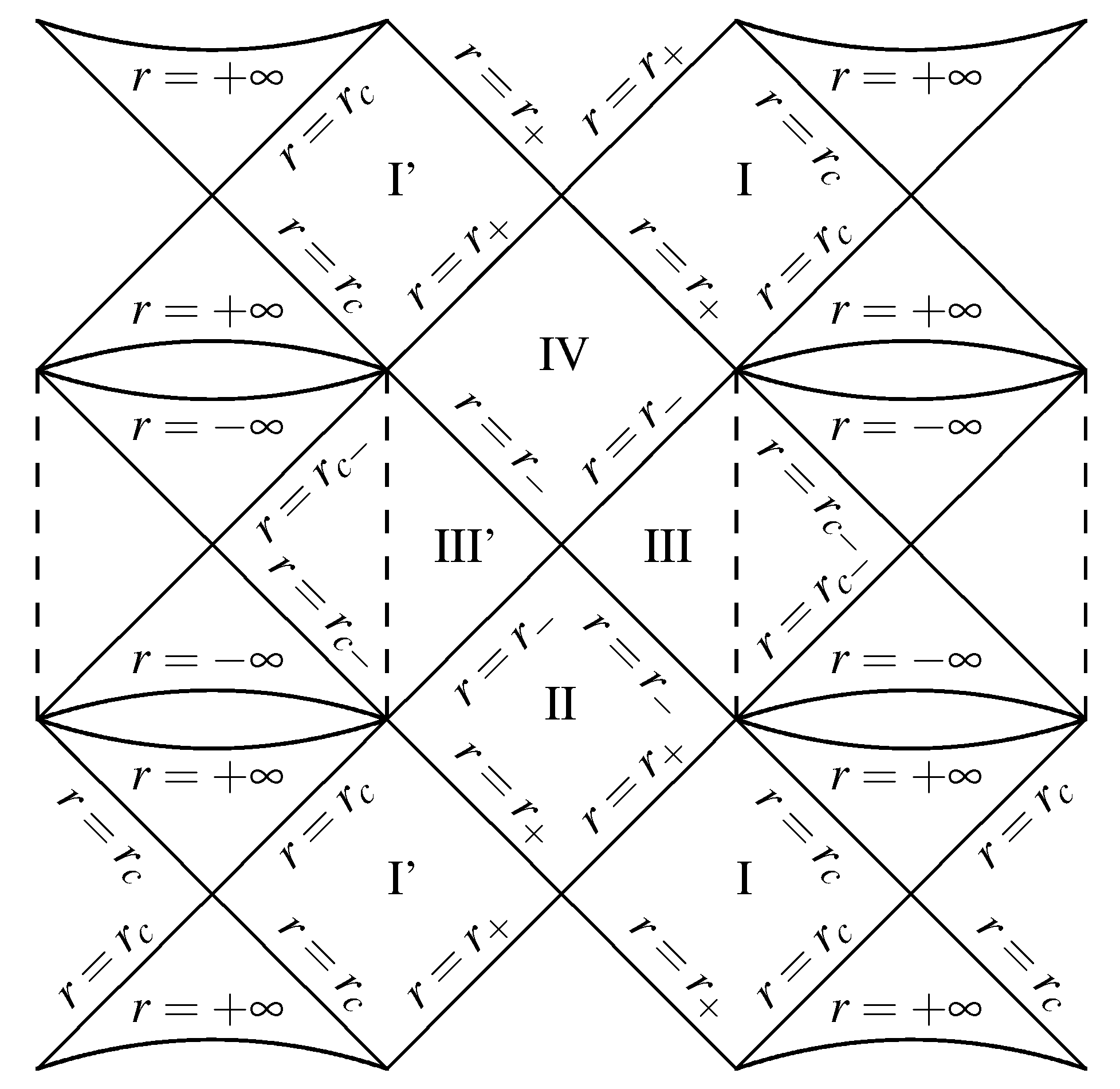
1.
The character of the geodesic motion in the complete Kerr–de Sitter spacetime and the relevance of the effective potential V ( - ) ( r ; L , a , y ) , governing particles in the negative-root states at the stationary region between the black-hole and cosmological horizons, is qualitatively the same as discussed in [62].
2.
For analogical estimates for primordial black holes and an effective cosmological constant related to vacuum energy density connected with the electroweak symmetry breaking or the quark confinement, see [16].
3.
Location of the “static radius” out of the equatorial plane is roughly given by its location in the SdS spacetime having the same cosmological parameter y < < 1 (relation (18)), as far away from the rotating black hole these two backgrounds almost coincide for y.
4.
It has been also shown recently that the Blandford–Znajek process [42] is closely related to the MPP [38].
5.
For the case of inclined magnetic field see [91].
6.
A similar approach is applied for oscillatory motion of string loops around black holes in [100,101].
7.
For detailed information on the so-called geodesic models of HF QPOs that could be related to binary systems containing both black holes or neutron stars, see [104].
8.
For exceptions related to Kerr naked singularities, see [105].
9.
In some sources, other frequency ratios are observed [102]—for example, in the active galactic nucleus XMMUJ134736.6+173403 at the Seyfert 2 galaxy SDSS J134736.39+173404.6, the frequency ratio 3:1 is exhibited [103] that could be also explained by the geodesic models of HF QPOs [110].
10.
We can consider the MPP as a general process relevant in any magnetic field around a rotating black hole, but, for the Blanford–Znajek process, a threshold magnetic field of high magnitude is necessary [38].
11.
Charged particles “kicked” from the ISCO at the equatorial plane and escaping to infinity were studied in [28,30].
12.
Note that the double or multi-toroidal structures can be constructed also in the model of uncharged hydrodynamical tori, in the framework of the so-called ringed accretion disks mixing relatively counter-rotating tori that could be created during evolution of accretion structures in active galactic nuclei [6,7,8,149,150].
13.
Of course, it would be instructive to consider both the terms in the right hand side of the Ohm law and combine the both limiting approaches. We plan such studies in future research.
Figure 1. Classification of the Kerr–de Sitter spacetimes governed by the existence of stable circular orbits of test particles in the equatorial plane. Dashed curve separates regions of black holes (BH) and naked singularities (NS), full curves separate spacetimes admitting either both families (±) of stable circular orbits or the plus-family (+) only or even no (0) stable circular orbits. Shaded is the region of stable counterrotating plus-family orbits.
Universe 06 00026 g001
Figure 2. The Penrose–Carter diagram of the maximal Kerr–de Sitter spacetime along the symmetry axis θ = 0 . The dashed vertical lines mark where the curvature ring singularities at r = 0 and θ = π / 2 occur. For r > 0 , there are three horizons: the cosmological horizon r c , the outer black-hole horizon r + and the inner black-hole horizon r - . For r < 0 , there is another cosmological horizon r c - and another infinity. The infinities at r = ± are not joined together. The conformal diagram continues ad infinitum in all direction [52,57].
Universe 06 00026 g002
Figure 3. Specific energy and specific angular momentum of the equatorial circular orbits of Kerr–de Sitter black-hole spacetimes. The spacetimes are specified by the cosmological parameter y = 10 - 5 and the rotational parameter a varying from 0 to 1 in steps of 0.2. The left column corresponds to the plus-family orbits, the right column corresponds to the minus-family orbits. The local extrema of the curves correspond to the marginally stable orbits.
Universe 06 00026 g003
Figure 4. Effective potential of the equatorial radial motion of test particles in the Kerr–de Sitter black-hole spacetime ( y = 10 - 4 , a 2 = 0.36 ) allowing stable circular orbits for corotating particles. Marginally bound (mb) orbits are given by the solid curve having two local maxima of the same value, corresponding to the inner [mb(i)] and the outer [mb(o)] marginally bound orbits. The dashed effective potential defines the inner marginally stable orbit [ms(i)] by coalescing the local minimum and the (inner) local maximum. Analogously, the dash-dotted potential defines the outer marginally stable orbit [ms(o)].
Universe 06 00026 g004
Figure 5. Mutual positions of astrophysically important circular orbits of the Kerr–de Sitter spacetime. The figure is constructed for the representative value of y = 2 × 10 - 5 . The radii of special equatorial circular orbits are plotted as functions of the rotational parameter a. The shaded region determines the black-hole (BH) part of the spacetime and the rest corresponds to the naked-singularity (NS) part. Solid curves are used for the plus-family orbits (in most cases, they correspond to the corotating orbits from the point of view of the locally nonrotating observers, but there are exceptions described in the text), while the dashed curves are used for the minus-family orbits (in all spacetimes under consideration: counterrotating orbits). Black curves determine the inner and outer black-hole horizons. Blue curves determine the photon circular orbits. Green curves determine the marginally bound circular orbits (there is a disconnection between BH and NS regions for the plus-family orbits). Orange curves determine the marginally stable orbits.
Universe 06 00026 g005
Figure 6. Keplerian specific angular momentum (orange curve) and effective potential of the photon geodesic motion (blue curve) of the Kerr–de Sitter black-hole spacetimes. In sub-figures (a-b) y = 10 - 4 and in (c-d) y = 10 - 5 , the rising (descending) part(s) of K + and the descending (rising) part(s) of K - correspond to the stable (unstable) orbits. The local extrema of the functions K ± determine the specific angular momentum of marginally stable orbits—the inner and the outer, ms ( i ) and ms ( o ) . The local extreme of the photon potential determines the impact parameter of the photon circular geodesic, ph ( c ) . Values of local extrema of both functions depend on spacetime parameters.
Universe 06 00026 g006
Figure 7. Equipotential surfaces (meridional sections) of the potential W ( r , θ ) in barotropic fluid orbiting a Kerr–de Sitter black hole. We show corotating fluid with uniform distribution of the specific angular momentum ( r , θ ) = c o n s t . Depending on , the character of critical equipotential self-crossing toroidal surfaces (red curve) is changed. The blue curve corresponds to the second critical equipotential (if it exists), which is opened. Regions of the potential values corresponding to the colored scales are only shown. Sub-figure (a) corresponds to accretion torus, sub-figure (b) to torus which is simultaneously accretion and excretion, sub-figures (c-d) correspond to excretion tori.
Universe 06 00026 g007
Figure 8. Maximally extended corotating and counterrotating tori around a Kerr–de Sitter (KdS) black hole, compared to an analogical torus around Schwarzschild–de Sitter (SdS) black hole. The corotating one is more extended.
Universe 06 00026 g008
Figure 9. Open equipotential surfaces of fluid toroidal structures around a Kerr–de Sitter black hole. These surfaces govern jets and demonstrate strong collimation while approaching the static radius of the spacetime and support the jet collimation in a distance much larger than the static radius. For comparison, the open equipotential surfaces are shown for the Kerr geometry where no collimation occurs.
Universe 06 00026 g009
Figure 10. Radial profiles of the frequencies of small harmonic oscillations ν θ , ν r and ν ϕ of charged particle orbiting a Kerr black hole of mass M = 10 M and spin a, immersed in an magnetic field characterized by the parameter B (various values of B from left to right).
Universe 06 00026 g010
Figure 11. Charged particle trajectory representing the chaotic scattering in the field of a magnetized black hole.
Universe 06 00026 g011
Figure 12. Thin Keplerian accretion disk around Schwarzschild BH in uniform magnetic field, created by neutral test particles following circular geodesics, and its evolution when the influence of the magnetic field is switched on. The accretion disk particles are following initially circular orbits with slight inclination from equatorial plane ( θ 0 = 1.5 ), while the magnetic field lines are everywhere aligned with the z-axis (vertical direction). The figures are labeled by the values of magnetic parameter B , as in the following corresponding figures generated for various values of spin a. The uncharged test particles on innermost stable spherical orbit (depicted by the dashed circle) represent the inner edge of the Keplerian accretion disk.
Universe 06 00026 g012
Figure 13. Thin Keplerian accretion disk around rotating Kerr BH ( a = 0.3 ) in uniform magnetic field. For a detailed description, see Figure 12.
Universe 06 00026 g013
Figure 14. Thin Keplerian accretion disk around rotating Kerr BH ( a = 0.7 ) in uniform magnetic field. For a detailed description, see Figure 12.
Universe 06 00026 g014
Figure 15. Thin Keplerian accretion disk around rotating Kerr BH ( a = 0.998 ) in uniform magnetic field. For a detailed description, see Figure 12.
Universe 06 00026 g015
Figure 16. Particle acceleration in the vicinity of a magnetized rotating black hole —1st neutral particle (black, neutron) has been located on accretion disk inner edge, decaying into two charged particles, 2nd (blue, proton), and 3rd (red, electron). While the 3rd particle (red) is trapped with large negative energy on orbits around black hole, the 2nd (blue) gets large energy due to the so-called chaotic scattering escapes along the magnetic field line.
Universe 06 00026 g016
Figure 17. Similar situation as in Figure 16, but here the magnetic field parameter B parameter is too small and the second particle will not escape.
Universe 06 00026 g017
Figure 18. Similar situation as in Figure 16, but here the magnetic field parameter B parameter is bigger and the second particle will escape with ultra-relativistic velocity.
Universe 06 00026 g018
Figure 19. Creation of Ultra-High-Energy Cosmic Rays. The left figure demonstrates the dependence of energy of protons accelerated by the MPP in the field of magnetized supermassive black hole with fixed mass in dependence on its spin and the intensity of the magnetic field. The right figure reflects a decrease of the proton energy due to the radiation reaction force working during its long-distance motion in weak intergalactic magnetic field with strength B 10 - 5 G. Notice that the energy decrease is similar to those related to the GZK process.
Universe 06 00026 g019
Figure 20. Representative comparison of trajectories of non-radiating (first line) and radiating (second line) charged particles around rotating Kerr black hole in a magnetic field. Initial conditions in both cases are chosen to be same and shown in the second row plots. The starting point is indicated by black dot. A radiating charged particle will radiate away its dynamical energy related to the Larmor precession and escape to infinity along magnetic field line aligned with the z-axis.
Universe 06 00026 g020
Figure 21. Typical behavior of the potential W for the charged fluid shown in terms of its poloidal profile (left) and poloidal equipotential contours (right). The behavior characterizes circulation of the fluid with 5.15 and K = A ϕ , in the dipole magnetic field with M = 2.6 . The twice self-crossing dashed curve determines the critical equatorial lobes with equatorial cusp and pseudo-cusp, corresponding to the equatorial saddle points; the dots denote locations of the cusp and pseudo-cusp.
Universe 06 00026 g021
Figure 22. Typical behavior of the potential W for the charged fluid shown in terms of its poloidal profile (left) and poloidal equipotential contours (right). The behavior characterizes circulation of the fluid with the 2.46 and K = A ϕ , in the dipole magnetic field with M - 1.17 . The self-crossing dot-dashed curve determines the pseudo-critical off-equatorial lobes with equatorial pseudo-cusp, corresponding to the equatorial saddle point, while the twice self-crossing dashed curve determines the critical cross-equatorial lobe with off-equatorial cusps, corresponding to the off-equatorial saddle points; the dots denote locations of the cusps and pseudo-cusp.
Universe 06 00026 g022
Figure 23. Typical behavior of the potential W for the charged fluid shown in terms of its poloidal equipotential contours—continuation of Figure 22.
Universe 06 00026 g023
Figure 24. Typical behavior of the potential W for the charged fluid shown in terms of its poloidal profile and poloidal equipotential contours. The behavior characterizes circulation of the fluid with 2.46 and K = A ϕ , in the dipole magnetic field with M - 0.95 . The twice self-crossing dashed curve determines the critical off-equatorial lobes with the off-equatorial cusps, corresponding to the off-equatorial saddle points, while the self-crossing dot-dashed curve determines the pseudo-critical off-equatorial lobes with the equatorial pseudo-cusp, corresponding to the equatorial saddle point; the dots denote locations of the cusps and pseudo-cusp.
Universe 06 00026 g024
Figure 25. Typical behavior of the potential W for the charged fluid shown in terms of its poloidal profile and poloidal equipotential contours. The behavior characterizes circulation of the fluid with Ω = - 1.6 × 10 - 3 and K = k A , where k = - 1.38 , in the field with the parameters a = 0.9 , B = 6.5 × 10 - 5 and Q = 3.99 × 10 - 3 . The twice self-crossing dot-dashed curve determines the pseudo-critical polar lobes with the equatorial pseudo-cusps, corresponding to the equatorial saddle points, while the twice self-crossing dashed curve determines the critical polar lobes with the polar cusps, corresponding to the polar saddle points; the dots denote locations of the cusps and pseudo-cusps.
Universe 06 00026 g025
Figure 26. Typical behavior of the potential W for the charged fluid shown in terms of its poloidal equipotential contours—continuation of Figure 25.
Universe 06 00026 g026
Figure 27. Typical behavior of the potential W for the charged fluid shown in terms of its poloidal profile (left) and poloidal equipotential contours (right). The behavior characterizes circulation of the fluid with Ω = - 1.6 × 10 - 3 and K = k A , where k = - 1.3 , in the field with the parameters a = 0.9 , B = 6.5 × 10 - 5 and Q = 3.99 × 10 - 3 . The twice self-crossing dashed curve determines the critical polar lobes with the polar cusps, corresponding to the polar saddle points, while the twice self-crossing dot-dashed curve determines the pseudo-critical polar lobes with the equatorial pseudo-cusps, corresponding to the equatorial saddle points; the dots denote locations of the cusps and pseudo-cusps.
Universe 06 00026 g027
Table 1. Mass parameter, the static radius and radii of the outer marginally stable and outer marginally bound circular orbits of the extreme KdS black-hole spacetimes with current value of the “relic” cosmological constant Λ 0 1.3 × 10 - 56 cm - 2 . Note that r ms ( o ) - < r ms ( o ) + , r mb ( o ) - < r mb ( o ) + as well as r mb ( o ) + < r s in general, but for presented values of the cosmological parameter y these pairs of radii are indistinguishable.
yM r s r ms ( o ) ± r mb ( o ) ±
[ M ][kpc][kpc][kpc]
10 - 44 100.230.150.23
10 - 40 1 × 10 3 1.10.671.1
10 - 34 1 × 10 6 116.711
10 - 28 1 × 10 9 1 . 1 × 10 2 67 1 . 1 × 10 2
10 - 26 1 × 10 10 2 . 3 × 10 2 1 . 5 × 10 2 2 . 3 × 10 2
10 - 24 1 × 10 11 5 . 0 × 10 2 3 . 1 × 10 2 5 . 0 × 10 2
10 - 22 1 × 10 12 1 . 1 × 10 3 6 . 7 × 10 2 1 . 1 × 10 3
Table 2. Intensity of the magnetic field B corresponding to the magnetic parameter B = 0.1 is given for various types of charged particles moving in the vicinity of the black hole of mass M BH 10 M .
M = 10 M /ElectronProtonFe+Charged Dust
B = 0 . 1 10 - 4 G 0 . 4 G 24 G 10 10 G
Table 3. The limits on mass M, given by optical measurements, and dimensionless spin a, given by spectral continuum fits, are presented along with the values of measured twin 3:2 HF QPOs for the three microquasars GRS 1915+105, XTE 1550-564 and GRO 1655-40.
Source f low [Hz] f L [Hz] f U [Hz]M [ M ]a
GRO 1655-40183004506.03–6.570.65–0.75
XTE 1550-564131842768.5–9.70.29–0.52
GRS 1915+1051011316810.6–14.4
Table 4. Magnitude of the magnetic field in the three microquasars implied by the fitting of the twin HF QPO frequencies. We use combined values for the ER variant of the magnetic modification of the geodesic model related to the 3:2 and 2:3 resonances (Table 3). Numbers in the table are in units of 10 - 5  G for electrons ( 2 × 10 - 2  G for protons).
GRO 1655-40XTE 1550-564GRS 1915+105
ER model
PALO11.5–23.08.2–16.30–14.5
RLOnoexist21.8–9.6–
PLO0–61.410.9–43.60– 28.9
RALO23.1–26.913.6–16.37.2–19.3
Table 5. Energy decay times of electrons ( τ e ) and protons ( τ p ) orbiting a black hole immersed in a uniform magnetic field with values of B characteristic for various astrophysical situations.
B (Gauss) τ e (s) τ p (s)
10 15     10 - 22       10 - 12   
10 12     10 - 16       10 - 6   
10 8     10 - 8       10 2   
10 4    1       10 10    
1    10 8        10 1    
10 - 5    10 18      10 28   

