A Test of Gravitational Theories Including Torsion with the BepiColombo Radio Science Experiment


1
IFAC-CNR, Via Madonna del Piano 10, 50019 Sesto Fiorentino (FI), Italy
2
Dipartimento di Matematica, Università di Pisa, Largo Bruno Pontecorvo 5, 56127 Pisa, Italy
*
Author to whom correspondence should be addressed.
Universe 2020, 6(10), 175; https://0-doi-org.brum.beds.ac.uk/10.3390/universe6100175
Submission received: 4 September 2020
/
Revised: 5 October 2020
/
Accepted: 9 October 2020
/
Published: 12 October 2020
(This article belongs to the Special Issue Universe: 5th Anniversary)
Abstract
:Within the framework of the relativity experiment of the ESA/JAXA BepiColombo mission to Mercury, which was launched at the end of 2018, we describe how a test of alternative theories of gravity, including torsion can be set up. Following March et al. (2011), the effects of a non-vanishing spacetime torsion have been parameterized by three torsion parameters, , , and . These parameters can be estimated within a global least squares fit, together with a number of parameters of interest, such as post-Newtonian parameters and , and the orbits of Mercury and the Earth. The simulations have been performed by means of the ORBIT14 orbit determination software, which was developed by the Celestial Mechanics Group of the University of Pisa for the analysis of the BepiColombo radio science experiment. We claim that the torsion parameters can be determined by means of the relativity experiment of BepiColombo at the level of some parts in , which is a significant result for constraining gravitational theories that allow spacetime torsion.
1. Introduction
Available experimental findings concerning gravitational interaction indicate that the Einstein’s General Theory of Relativity (GR) is presently the most suitable theory of gravitation. According to GR, the flat Minkowsky spacetime is deformed by the matter, giving rise to a non-flat and dynamic spacetime, tied by Riemannian geometry. On the other hand, it is well-known that the other fundamental interactions can be successfully described, at the microscopic level, within a rigid and flat spacetime. Because GR was originally formulated as a theory involving mass distribution at macroscopic level, it is desirable to consider suitable generalizations of GR that include micro-physical processes, which could possibly induce macroscopic effects, to be constrained, in turn, by experiments (cfr., e.g., the discussion in [1]).
In the following, we will consider a particular generalization of GR, which includes a non-vanishing spacetime torsion. Elementary particles, which constitute matter, are characterized by their intrinsic spin. Because spin averages out at macroscopic level, GR considers that the dynamical behavior of a macroscopic distribution of mass can be described by the energy-momentum tensor of matter alone, which is coupled to the metric of a Riemann spacetime. However, at the microscopic level, the spin angular momentum also plays a role in the dynamics, thus it must be coupled in some way to spacetime. This fact leads to the formulation of a more general spacetime, the four-dimensional Riemann–Cartan spacetime, which is characterized by an additional, non-Riemannian part of the affine connection, called the contorsion tensor, which should be coupled to the spin (see, e.g., [1,2]).
Torsion, as the anti-symmetric part of an asymmetric affine connection, was firstly introduced one century ago by Élie Cartan [3], who glimpsed the link between spacetime torsion and intrinsic angular momentum of matter (for an historical perspective see, e.g., [1]). If torsion is admitted, then it might affect spinning particles and, thus, indirectly, act on light and test particles throughout the field equations, which determine the metric. Most of the torsion theories predict a negligible amount of torsion in the solar system [4]. Indeed, beyond GR, theories of gravitation usually assume that torsion only couples to the intrinsic spin of particles and not to rotational angular momentum (see, e.g., [5]).
Recently, Mao et al. [6] considered the issue from another point of view: given an experiment to test gravitational theories in the solar system, the problem could be modeled by means of a non-standard gravitational Lagrangian, which includes a detectable torsion signal. Subsequently, whether the model is in agreement or not with the data can be experimentally tested. Later on, March et al. [7] developed a more general framework, within the scope of the parameterized post-Newtonian (PPN) approximation (see, e.g., [8]), in order to test the possible effects due to torsion around massive bodies in the solar system.
In this perspective, the radio science experiment on-board the BepiColombo mission to Mercury gives an intriguing opportunity to test possible modifications of GR in the solar system. BepiColombo is an ESA/JAXA mission that was launched in October 2018. The mission aims at a comprehensive exploration of the planet Mercury, thanks to two spacecraft, whose orbit insertion around the planet is expected for the end of 2025 [9]. The Mercury Orbiter Radio science Experiment (MORE) is one of the on-board experiments, which is devised to enable a better understanding of the geodesy and geophysics of Mercury, on one side, and of fundamental physics, on the other (see, e.g., [10,11,12]). Thanks to full on-board and on-ground instrumentation capable to perform very precise tracking from the Earth, MORE will have the chance to determine, with very high accuracy, the Mercury-centric orbit of the spacecraft and the heliocentric orbit of Mercury and the Earth. Taking advantage of the fact that Mercury is the nearest planet to the Sun, MORE will allow for an accurate test of relativistic theories of gravitation (“relativity experiment”). The test consists of simultaneously constraining the value of a number of parameters that describe the parameterized post-Newtonian (PPN) framework together with some other parameters of general interest, by means of a global non-linear least squares fit. This can be achieved, as will be described later, employing a dedicated orbit determination OD software, ORBIT14, which was developed at the University of Pisa.
The paper is organized, as follows. In Section 2, we briefly describe the MORE relativity experiment: we present the dynamical model and discuss the adopted mathematical methods, together with some generalities on the ORBIT14 software. In Section 3, we describe the generalization of the dynamical model, including the possible effects due to spacetime torsion and we illustrate the implementation of torsion in the software. In Section 4, we present and discuss the results of the numerical simulations of the MORE relativity experiment, focusing on the torsion parameters. Finally, in Section 5, we outline some conclusions.
2. MORE Relativity Experiment
Mercury is the inner planet of the solar system; hence, it is the most sensitive to the gravitational effects of the Sun. Consequently, it is a long-established fact that a space mission to Mercury would significantly improve the determination of the PPN parameters, more tightly constraining their agreement, or disagreement, with GR predictions [13]. The BepiColombo opportunity precisely suits this scope, since it is equipped with on-board instrumentation that is capable of very precise tracking from the Earth [14] in order to perform a comprehensive radio science experiment (MORE), consisting of a gravimetry, a rotation, and a relativity experiment.
The global experiment aims at determining the following quantities of general interest:
- the parameters defining the model of Mercury’s rotation (“rotation experiment”, all of the details can be found in [17]);
- the “relativity” parameters, which are the PPN parameters , , , and the Nordtvedt parameter , which characterize the expansion of the spacetime metric in the limit of slow motion and weak field (see, e.g., [8,18])1, together with some related parameters, such as the oblateness of the Sun , the solar gravitational mass (where G is the gravitational constant and the mass of the Sun), possibly its time derivative , and the solar angular momentum which appears in the Lense–Thirring effect on the orbit of Mercury (see, e.g., [19,20,21] for a general discussion; moreover, the topic has been addressed by the authors in the case of MORE in [22]).
In order to achieve the challenging scientific goals of MORE, it is mandatory to perform a very precise determination of the orbit of the spacecraft around Mercury and of the orbit of Mercury and the Earth. In fact, in our analysis, the orbit determination is performed with respect to the Earth-Moon barycenter (EMB) instead of the Earth; this approach can be adopted, since the orbit of the Moon is known to the cm-level thanks to the lunar laser ranging (LLR). Orbit determination is enabled, in turn, by state-of-the-art on-board and on-ground instrumentation [14,23]. The on-board transponder will be able to collect the radio tracking observables (range, range-rate) up to a goal accuracy (in Ka-band) of approximately cm at 300 s for one-way range and cm/s at 1000 s for one-way range-rate.
2.1. The Heliocentric Dynamics of Mercury and the EMB
To perform the OD of the spacecraft, Mercury, and the EMB at the required level of accuracy, their dynamics need to be modeled very carefully. In practice, although we are dealing with a unique global experiment and a unique set of measurements, we can conceptually separate the gravimetry-rotation experiments from the relativity experiment (see, e.g., [24]). As a matter of fact, gravimetry and rotation mainly involve short period phenomena, being preferentially related to the orbital motion of the spacecraft around Mercury (which has a periodicity of 2.3 h). On the other hand, relativistic phenomena take place over longer time scales, of the order of months or years, thus they can be mainly analyzed by studying the heliocentric motion of Mercury and the Earth, taking place over 88 and 365 days, respectively. Furthermore, the chance to perform the relativity experiment independently from the others, for the purpose of simulations, is even more legitimate if we consider the goal accuracies of the observations: properly comparing and over the same integration time according to Gaussian statistics, we find that s. Thus, we can infer that range observations are more accurate when observing phenomena with periodicity longer than s, like relativistic phenomena, while the opposite holds for gravimetry and rotation, which are, in turn, mainly performed by means of range-rate observations.
All of the details concerning the Mercury-centric dynamical model of the spacecraft can be found in [24,25]. In the following, we will focus on the heliocentric dynamics of Mercury and the EMB, which, in fact, represent the core of the MORE relativity experiment. Adopting a Lagrangian formulation, the equation of motion for Mercury and EMB are given by the Euler–Lagrange equations:
where , are position and velocity, respectively, of the i-th body ( for Mercury, for EMB) computed in the solar system barycenter (SSB) reference frame and L is the Lagrangian of the problem. The Lagrangian can be decomposed, in turn, as
where is the Lagrangian of the Newtonian N-body problem, is the correction due to GR in the PPN limit, and includes the contribution due to PN and related parameters. In particular, the term describes how each parameter individually affects the dynamics and it assumes the form:
The explicit expression of each term appearing in Equation (2) can be found in [24]. Let us recall that and are expected to be equal to unit in GR, while , and are null in GR.
The total acceleration acting on the i-th body can be derived from Equation (1), while taking into account that the main term is the N-body Newtonian acceleration, , while the other terms are small perturbations. It takes the following approximated expression:
where accounts for the acceleration of the SSB (see [24] for details).
2.2. Mathematical Methods
The parameters of interest for the MORE relativity experiment are simultaneously determined by means of a global non-linear least squares (LS) fit. Following, e.g., [15]—Chapter 5, the non-linear LS fit aims at determining a set of parameters, , which minimizes the target function:
where m is the number of observations, W is the matrix containing the observation weights and is the vector of the residuals, which is the difference between the observations (i.e., the tracking data) and the predictions , resulting from the light-time computation as a function of all the parameters (see [26] for all of the details).
The procedure to compute the set of the parameters that minimizes Q is based on a modified Newton’s method, called the differential correction method. First, we define the design matrix B and the normal matrix C as
The stationary points of the target function are the solution of the normal equation:
where . The method consists in applying iteratively the correction
until convergence. We always adopt the probabilistic interpretation of the inverse of the normal matrix, , as the covariance matrix of the vector , considered as a multivariate Gaussian distribution with mean in the space of the parameters (see, e.g., [15]—Chapter 3). In particular, the diagonal terms of carry the information on the attainable precision by which the parameters can be estimated, which we will refer to as “formal accuracy” in the following.
When some information on one or more solve-for parameters is available, it should be taken into account during the differential correction process. Let us suppose that some information on each of the N solve-for parameters is provided by some source (past space missions, ground-based gravimetry, etc.) and let be the apriori values of the solve-for parameters. An apriori standard deviation is associated with each apriori observation, (). If , then this is equivalent to the normal equation . The target function is modified to take the apriori information into account, thus becoming
Finally, the new normal system is
Note that the same formulae can be used in case a subset of the solve-for parameters satisfies a number k of linear relations2 Let be the linear system expressing such linear relations. In this case, the apriori normal matrix is defined as
where is the matrix of the apriori weights.
2.3. The ORBIT14 Software
Since 2007, the Celestial Mechanics Group of the University of Pisa has developed (under an Italian Space Agency agreement) an orbit determination software, ORBIT14, dedicated to the BepiColombo and Juno radio science experiments (see, e.g., [27,28]). All the code is written in Fortran90.
In the case of BepiColombo, the software includes two separated stages:
- the data simulator: awaiting for real data, it generates the simulated observables and the nominal value for the orbital elements of the Mercury-centric orbit of the spacecraft and the heliocentric orbits of Mercury and the EMB; and,
- the differential corrector: it is the core of the code, solving for the parameters of interest by means of a global non-linear LS fit, within a constrained multi-arc strategy [29].
3. Dynamical Model with Torsion
Most torsion theories predict a negligible amount of torsion in the solar system, as briefly mentioned in the Introduction. In many theories, torsion is non-propagating, since torsion is related to its source via an algebraic equation rather than a differential one. Nevertheless, also in theories that allow for torsion to propagate, it is usually assumed that it only couples with intrinsic spin and not to rotational angular momentum, thus becoming negligibly small at macroscopic level3.
Overturning the issue, without referring to any particular theory of gravitation, we can ask if a rotating planet in the solar system could generate torsion and if this fact could produce experimentally detectable effects. The possible presence of torsion can be tested in our framework by providing a Lagrangian formulation of the problem, i.e., by adding a new term to Equation (2), which accounts for torsion effects. In the following, we will refer to the work of [7] in order to build a proper Lagrangian term that accounts for spacetime torsion. In the future, models with different assumptions should be similarly tested with the ORBIT14 software.
Following [7], we will consider a class of gravitational theories allowing for non-vanishing torsion that is based on a Riemann–Cartan spacetime. This spacetime is a four-dimensional manifold endowed with a Lorentzian metric and an affine connection such that (mathematical details can be found, e.g., in [1]). The connection is uniquely determined by the metric and torsion tensor:
In this case, the connection departs from the Levi–Civita connection (which is symmetric in the first two indices and holds in the Riemann spacetime of GR) by an additional anti-symmetric term, called the contorsion tensor, , which cancels out in the case of vanishing torsion tensor.
3.1. Spacetime with Torsion in a PPN Framework
In order to develop a model to test torsion within a PPN framework that is consistent with the dynamical model described in Section 2.1, the metric and the torsion tensor need to be parameterized in a region of space at a distance r from the Sun, such that the quantity , i.e., at large distances when compared with the Schwarzschild radius. Because the PPN framework we are adopting includes terms up to second order in the small quantity (see, e.g., [6,7]), the metric and the torsion tensor must be expanded up to the same degree of accuracy.
In general, the torsion tensor has 24 independent components, each being a function of time and position, but adopting symmetry arguments and a perturbative approach up to , March et al. [7] showed that there are only 2 independent components of the torsion tensor, which can be parameterized as a function of four independent dimensionless constants, , , , and , as (see [7] for details):
where are a set of non-isotropic spherical coordinates, as defined in [7]. Therefore, the connection becomes an explicit function of the torsion parameters , , , and . Moreover, because the metric and the connection are such that the condition is satisfied, it follows that the metric is independent of the torsion parameters.
Once the non-vanishing components of the connection up to are derived (see [7]—Equation (5.1)), the system of the equations of motion can be built. In particular, Ref. [7] found that, at the required level of accuracy, the dependency of the connection components on can be neglected; thus, finally, the spacetime torsion in our model can be parameterized by means of only three torsion parameters: , , .
In a Riemann-Cartan spacetime, two different classes of curves can be considered, autoparallels and geodesics curves, which reduce both to the geodesics of the Riemann spacetime when torsion vanishes [1]. In particular, autoparallels are curves along which the velocity vector is transported parallel to itself by the connection , while, along geodesics, the velocity vector is transported parallel to itself by the Levi-Civita connection. In GR, the two types of trajectories coincide, while, in general, they may differ in the presence of torsion. Because geodesics curves in this generalized framework turn out to be the same as in the standard PPN framework (see [7] for details), new predictions that are related to torsion may only arise when considering autoparallel trajectories, which explicitly depend on torsion parameters.
Hence, we assume that the test body (in our case either Mercury or the Earth, neglecting their internal structure) moves along an autoparallel trajectory4. The equation of motion along an autoparallel curve has the following general form:
where is the proper time. After some mathematical manipulations and simplifications and only accounting for terms up to the second order in the small quantity , March et al. [7] achieved the final equation of motion for a test body moving along an autoparallel trajectory, written in rectangular coordinates:
where , , and m is the mass of the central massive body ( has been assumed)5. We also recall that, differently from our approach, in [7] all of the PPN parameters other than and are assumed to be zero; hence, they are not included in the development and parameterization of the metric and the connection.
3.2. Implementation of Torsion in ORBIT14
To properly account for the possible dynamical effects due to spacetime torsion, we need to add the torsion contribution to the global acceleration acting on the i-th body, as described by Equation (3). In principle, we could directly use Equation (6), but, for the purposes of the MORE relativity experiment, we need to take rhe possible dynamical effects into account due to all of the PPN and related parameters that we are interested in, since they all need to be determined simultaneously in the LS fit. Nevertheless, assuming that the only contribution to the Lagrangian is due to and , Equations (3) and (6) must coincide apart from the terms due to torsion. This, in fact, is the case; thus, after some manipulation, we can isolate the contribution due to torsion on the motion of the i-th body, which reads 6:
where is the position of the body i with respect to the SSB and is its module (the same notation holding for the velocity vector).
Two issues stand out by looking at Equation (7). The first one concerns the fact that the contribution to the acceleration due to each of the three torsion parameters depends on the gravitational mass of the Sun, , which is also one of the parameters to be determined; in the case of , also a coupling with occurs. Thus, we need to properly take this dependency in the computation of the design and normal matrices into account, which must contain the partial derivatives of the new acceleration term with respect to and . As a consequence, we can expect that a considerable correlation between , and the torsion parameters could show up by simultaneously solving for all of the parameters.
The second issue specifically concerns and . Looking at Equation (6), it turns out that the dynamical effect due to these two parameters shows the same proportionality to the term . Thus, we can define an overall acceleration term due to the combined effect of both parameters, as given by:
As a consequence, in principle, we cannot simultaneously solve for the two parameters within the LS fit, since the observable signature due to one parameter cannot be distinguished from the other. From a computational point of view, this means that the design matrix would have two linearly dependent columns, so that the normal matrix would be degenerate, hence not invertible. This circumstance is known in the literature as rank deficiency and a general description of the issue in the case of an OD problem can be found in [15]—Chapter 6. Similar issues have been already dealt with in the past in the framework of the MORE relativity experiment (a detailed discussion on the approximate rank deficiency between and the oblateness of the Sun, , can be found in [11], while the general issue in the case of the MORE relativity experiment has been widely discussed by the authors in [22,28]).
Rank deficiencies in an OD problem can be cured in two ways: solving fewer parameters (this technique is known as descoping) or using more observations. The second way can be pursued by adding independent observations (e.g., using data from other experiments [31]) or, similarly, by adding a number of constraints equal to the order of the rank deficiency, which represent the available apriori knowledge of the problem (see, e.g., [22]). The first approach (descoping) has been applied; in fact, in the framework of the relativity experiment until now: assuming a vanishing torsion, as in GR, is equivalent to the assumption that ; thus, looking at Equation (8), the actual effect on the dynamics is all due to the parameter . This will be the strategy applied in the scenarios of the reference simulation and of simulation (a) described in Section 4.2. On the other hand, if we consider that a non-vanishing torsion may exist and, in particular, could be not null, the descoping approach cannot be adopted anymore. In this case, we cannot separate the effects of and , and we can only estimate the linear combination . If we aim at determining both parameters, then we need to add some further information on, at least, one of the two parameters. This can be done by adding an apriori constraint on the parameter , as given by the present knowledge on its value. If the apriori constraint is sufficiently tight, then the normal matrix can be inverted again and the problem can be solved. This approach will be adopted in the case of simulation (b) in Section 4.2.
4. Numerical Analysis
In this Section, we describe the results of the numerical simulations of the MORE relativity experiment, including the dynamical effects due to torsion. In particular, we aim at checking whether the torsion parameters can be estimated by means of the experiment and, if so, at which level of accuracy.
4.1. Simulation Scenario and Assumptions
First of all, we define a reference scenario. In this case, the LS fit aims at determining the relativity parameters that are listed in Section 2, without accounting for the possible effects due to torsion in the solution (see, e.g., [22]). We recall that the relativity parameters are: the PPN parameters , , , , the Nordtvedt parameter , the oblateness of the Sun , the gravitational mass of the Sun , its time derivative , and the angular momentum of the Sun . We point out that, for the purposes of this work, we do not include in the solve-for list the gravimetry and rotation parameters that are introduced in Section 2. As a matter of fact, while a global solution solving simultaneously for all of the parameters will be performed when dealing with real data, for the goal of simulations we can consider the relativity and related parameters alone, since we extensively verified in the past (see, e.g., [24]) that they are not correlated at all with the gravimetry-rotation parameters, thus the solution is not invalidated by removing these last parameters from the solve-for list.
The starting epoch of the simulation is set to 14 March 2026 and the nominal duration is set to one year. In Section 4.4, we will also consider the possible benefits due to an extension of the mission duration up to an additional year. We assume that the radio tracking observables are only affected by random effects with a standard deviation of cm at 300 s and cm/s at 1000 s, respectively, for Ka-band observations. The software is capable of also including a possible systematic component to the range error model and to calibrate for it, but, since we are interested in a covariance analysis, we do not account for this detrimental effect here (this issue has been partially discussed in [32]).
For each relativity parameter that we are interested in, we set an apriori constraint given by the present knowledge of the parameter, as listed in Table 1. We point out that the adopted apriori on is a conservative estimate that is derived by a full set of simulations, carried out by the authors in [33], of the Superior Conjunction Experiment (SCE), planned during the cruise phase of BepiColombo 7. Concerning the torsion parameters, they have not been experimentally estimated so far. In [7], referring to the present knowledge of and , the authors derived the following constraints on the values of and :
Moreover, we make use of an important assumption: we link the PN parameters by the Nordtvedt equation [34]
which means that we are only considering metric theories of gravitation. The addition of the Nordtvedt equation in our model is motivated by the fact that and are expected to show an almost 100% correlation, since their dynamical effect on the orbit of Mercury is comparable (see, e.g., [11] for an extensive discussion of this symmetry in the case of the MORE relativity experiment). Thus, the addition of the constraint removes the degeneracy between and , but this result is, in turn, obtained at the cost of forcing an almost 100% correlation between and 8.
4.2. Simulation Results
In the following, we denote “reference simulation” as the case in which the solution is computed in the standard reference scenario that is described in Section 4.1, which consists in estimating the state vectors of Mercury and the EMB at the central epoch of the mission (6 plus six parameters) and the relativity parameters, for a total of 21 parameters. Subsequently, we define as simulation (a) the case of the reference scenario with the addition of the torsion parameters and in the solve-for list, for a total of 23 estimated parameters, and we estimate in place of . Finally, we label as simulation (b) the case of a simulation in which all three torsion parameters, , , and , are simultaneously determined by means of the LS fit together with the relativity parameters and the state vectors, for a total of 24 parameters. In addition, in each scenario the state vector of the spacecraft (position and velocity, 6 parameters) is estimated at the central epoch of each of the 365 observed arcs, for a total of 2190 parameters. These parameters are handled as local parameters (i.e., they belong only to a single arc: see, e.g., [29] for details) and they result in being uncorrelated with the relativity parameters, which are global parameters. For the sake of clarity, the global parameters that are estimated in each of the three scenarios are summarized in Table 2.
The results in terms of formal accuracies (1-) determined in the three different scenarios are compared in Table 3 for what concerns the state vectors (position and velocity in cartesian coordinates) of Mercury (labeled with the index M) and the EMB (labeled with the index E), while, in Table 4, the corresponding results for the relativity parameters are shown. We point out that at this stage we are only interested in the formal accuracy with which each parameter can be determined, since we are running a purely formal analysis with the aim of testing if torsion parameters can be included in our fit or not. This means that we are not interested in estimating the central value of each parameter, which will be, instead, the task of the analysis of real data. Indeed, because we are using simulated data, the estimated values are meaningless (i.e., they merely depend on the simulation assumptions and adopted nominal values). In particular, we did not include any source of systematic error in our simulations, which could be “absorbed” by some parameters, leading to a bias in their central value (see, e.g., [32]) for a discussion of this issue). As a consequence, while we checked that convergence in this framework is reached in few iterations, the accuracy by which each parameters can be estimated is provided by the diagonal terms of the covariance matrix already after the first iteration of the non-linear LS fit and it does not vary significantly throughout the following iterations.
Concerning the determination of the state vectors at the central epoch, as shown in Table 3, we can immediately observe that, as expected, the results do not vary depending on the scenario. This suggests that the there is no correlation between the torsion parameters and any of the components of the orbital conditions of Mercury and the EMB, i.e., solving for the torsion parameters does not weaken the determination of the state vectors. The two orbits can be determined with the MORE experiment at the level of some meters, for what concerns the position, and of some m/s, concerning the velocity, with a general trend of a better estimate in the x-y plane, while the z-direction seems weaker. We point out that no constraint has been imposed on the two orbits (contrarily to what the authors have done in [22]): the issue of possible symmetries affecting the geometry of our experiment is very critical and a dedicated paper will be devoted by the authors to this specific topic in the near future.
Moving attention to Table 4, first of all some observations on the results that are achievable in the case of the reference scenario are in order. When comparing the estimated accuracy with the present knowledge, shown in Table 1, we can expect that the MORE experiment will provide a significant improvement in the knowledge of , , and . In particular, in the case of , we point out that the experiment allows to determine the parameter at the level of the theoretical constraint computed by Nordtvedt in [40], which is , while the apriori constraint we set on , which is [38], as shown in Table 1, is derived by measurements in the solar system. A minor improvement could be achieved in the estimate of the gravitational mass of the Sun, , while no significant improvement is expected, at the moment, for the knowledge of (see [24] for a discussion regarding this parameter) and (see [22] for a further discussion).
Concerning the torsion parameters, which are the focus of this work, we can observe that, in the case of simulation (a), we achieve the relevant result that the torsion parameters and can be estimated by means of the MORE relativity experiment at the level of , which could place a significant constraint on the validity or not of torsion theories. In the case of simulation (b), i.e. also estimating the parameter , an order of magnitude is lost in the determination of the torsion parameters. This is mainly a consequence of the strong correlation between and : since the three torsion parameters are expected to be correlated one with the other (see Equation (7)), the worsening affects the estimate of all the three parameters. Anyway, they can be estimated at the level of some parts in and this is still a remarkable result.
The addition of the torsion parameters in the solve-for list worsens the determination of most of the relativity parameters, slightly more in the case of simulation (b) with respect to simulation (a). The worsening is more pronounced in the case of the parameter , whose accuracy deteriorates by a factor 3 in simulation (a) and by a factor 4 in simulation (b). This result is not surprising, since the dynamical effect due to torsion depends on , as pointed out in Section 3.2. In particular, in the case of simulation (b), the accuracy of the parameter is comparable to the present knowledge, and this fact suggests that, in the absence of an apriori on , it would be difficult to solve this parameter simultaneously with the torsion parameters. In the case of the parameters and , the worsening is limited by less than a factor 2. This fact may seem to be contradictory in the case of simulation (b). Indeed, in Section 3.2, we have seen that the dynamical effect due to and is the same and, as a consequence, we could expect that the addition of in the solve-for list should cause a significant worsening in the determination of . This is, in fact, the case: if we do not constrain the value of in some way and we simultaneously estimate , thenwe would find that the normal matrix is not invertible. The problem is solved by adding the present knowledge on as an apriori constraint on the parameter: we are not able to improve the present knowledge of (by looking at Table 4—simulation (b), the achievable formal accuracy is equal to the present knowledge), but at least we are able to separate its effect from that of .
A special discussion deserves the issue of the determination itself of and . We recall that the two parameters are highly correlated, since they are linked through the Nordtvedt relation. In the past, we observed that the determination of and strongly depends on the level at which the experiment is capable to determine the orbits of Mercury and the EMB. In particular, referring to the results that are shown in [22], we observed that the determination of the orbits of Mercury and the EMB with an accuracy below the meter and m/s for the position and velocity, respectively, leads to a great benefit in the estimate of and (cf. Tables 2 and 3 in [22]). The problem is that an accuracy at the level of 10 cm or less in the determination of the two orbits seems unrealistic, due to a number of detrimental effects, in particular due to the uncertainty in the knowledge of the masses and state vectors of the bodies in the solar system, which influences, in turn, the position and velocity of Mercury and the EMB (mainly in the case of Jupiter, see [41] for an extensive discussion). Indeed, we point out that, for the purpose of the experiment, the mass and position of the bodies included in the N-body Newtonian acceleration (see Equation (3)) are taken from the JPL ephemerides, thus they are assumed to be perfectly known. As a consequence, we cannot expect to significantly improve our knowledge on and with the relativity experiment set up in the way described here. Different choices can be made, when considering a wider set of independent observations due to different space missions to be fitted simultaneously, as proposed in [31]. In particular, in [42], the authors deal with the issue of accounting for all of the other bodies in the solar system in the Mercury orbit determination problem of the NASA MESSENGER mission. They point out that the orbit of Mercury cannot be determined at the desired level of accuracy with a radio science experiment from the Earth, which assumes an Earth-Mercury-Sun isolated system. On the other hand, our purpose is to show that the torsion parameters can be estimated in our set-up and focus on how their presence can affect the estimate of the other parameters. In the perspective of the orbital phase of the BepiColombo mission, in 2026, we are aware that the assumption of a three-body isolated system could lead to misleading results, in particular on the determination of and .
4.3. Analysis of the Correlations
The correlations showing up between the estimated parameters need to be analyzed in order to carry out a complete description of the results. We recall that the correlation of the parameter A with the parameter B, , where A and B are, respectively, the i-th and the j-th parameters in the solve-for list, is proportional to the out-of-diagonal term of the covariance matrix (see Section 2.2) and it is normalized to 1 by means of the formal accuracy of the two parameters, and .
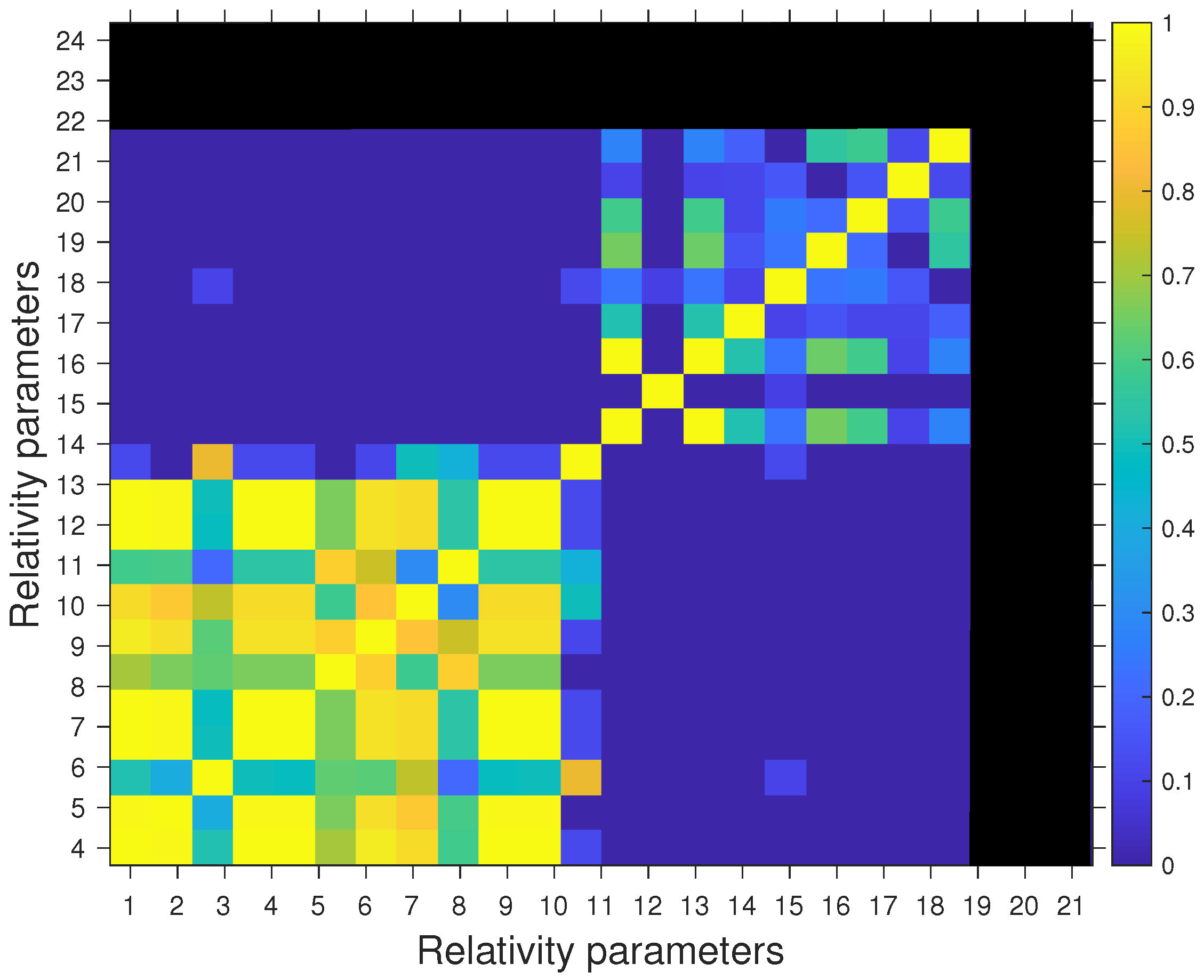
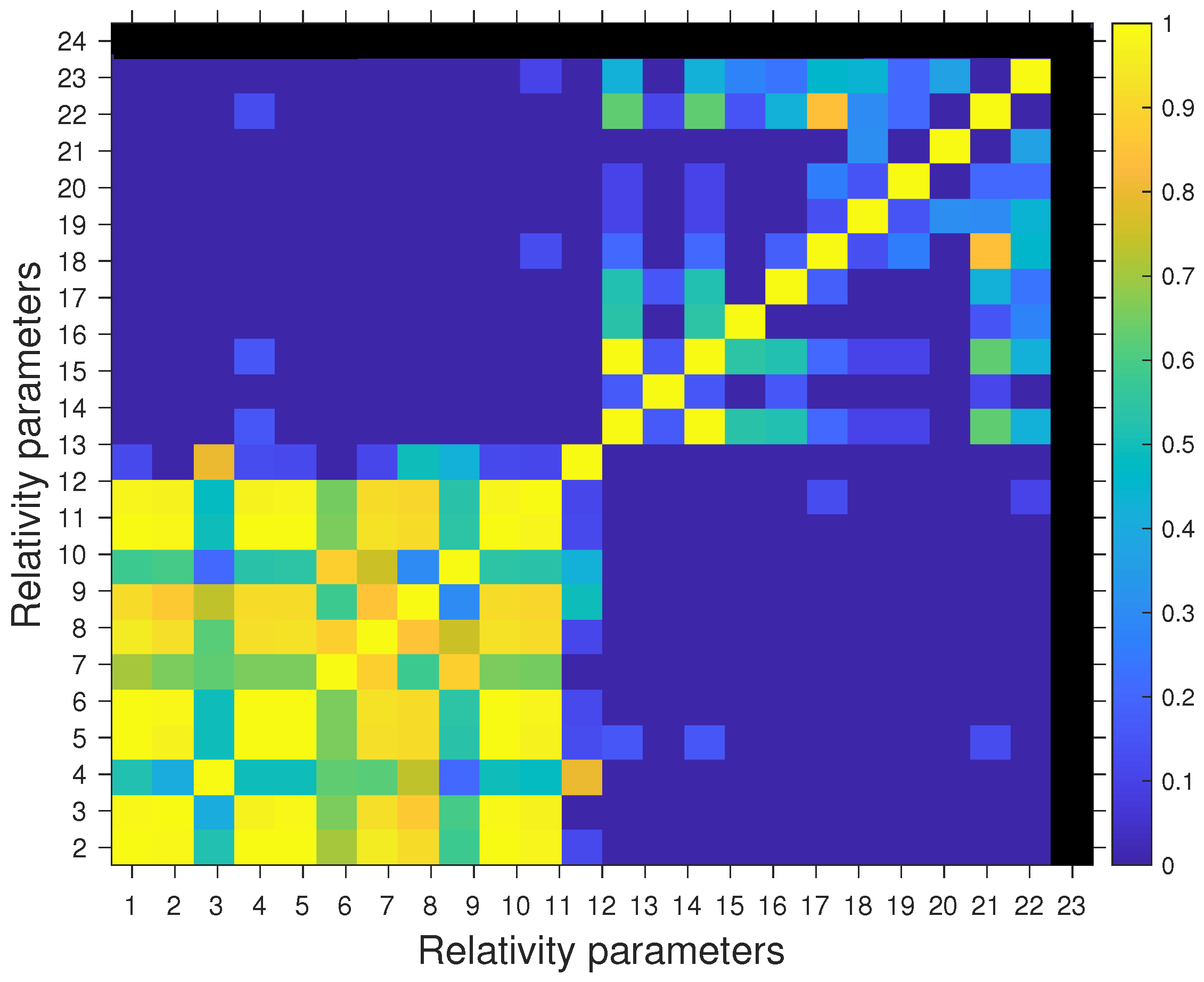
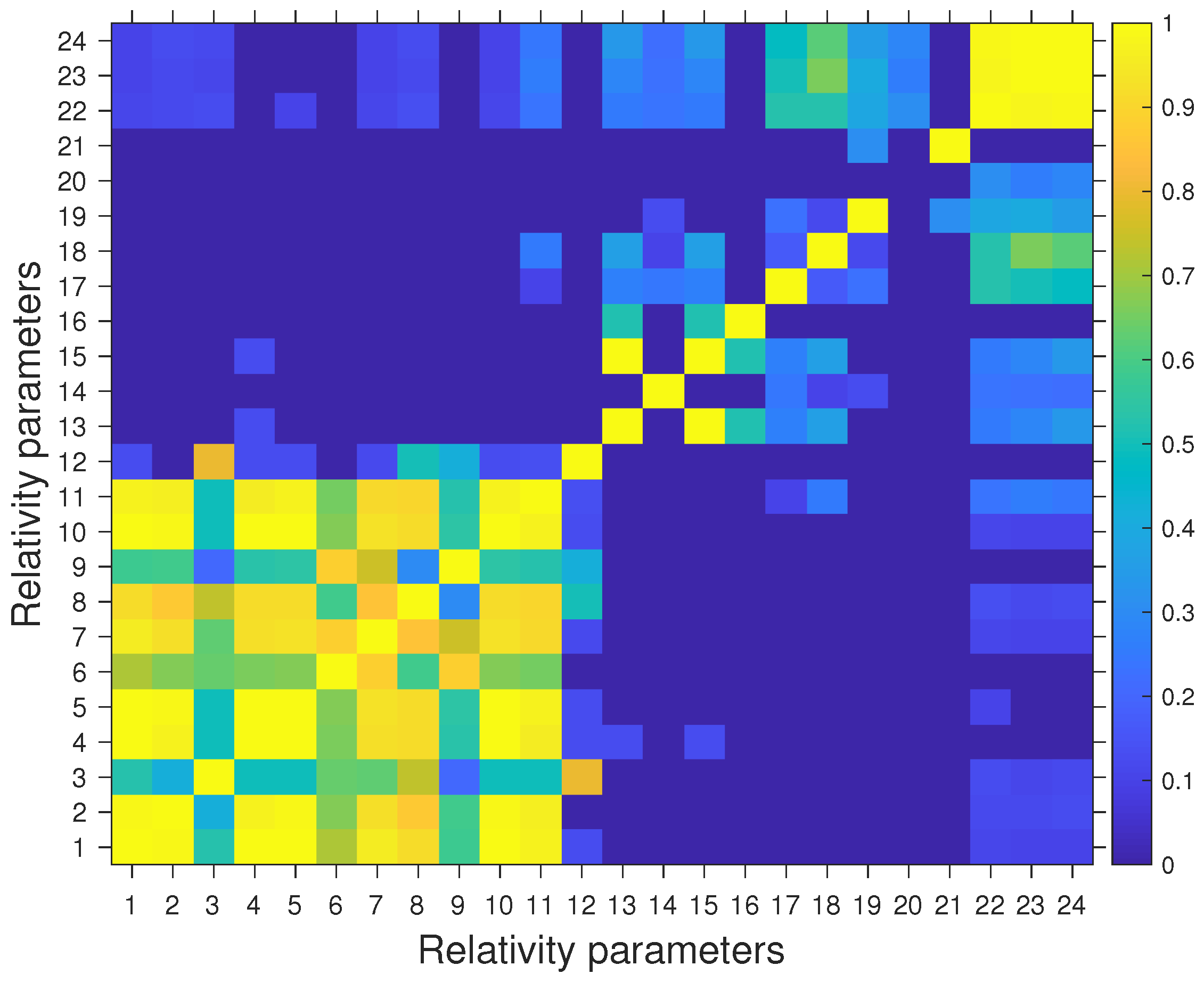
A global view of the behavior of correlations between the parameters is given in Figure 1, Figure 2 and Figure 3 for the cases of the reference simulation, simulation (a), and simulation (b), respectively. The estimated parameters are labeled with a number , as in Table 3 and Table 4: indices from 1 to 12 refer to the state vectors of Mercury and the EMB (position and velocity components), from 13 to 21 to the relativity parameters, in the order indicated in Table 4, and, finally, from 22 to 24 to the three torsion parameters. The color-bar on the right of each figure spans from the value 0 (dark blue) in the case that no correlation is found to the value 1 (yellow) in the case that an exact correlation shows up.
In the case of the reference simulation (Figure 1), a two-block structure can be clearly recognized, which can be found also in the cases of simulation (a) and (b). This structure reveals the fact that the subset of parameters 1–12, i.e., the components of the state vectors, and the subset of the parameters 13–21, i.e., the relativity parameters are almost not correlated one with the others, while one parameter can only be highly correlated with the other parameters of the same subset. In particular, we can observe that the correlation between and is in all the three cases, as expected. Moreover, shows a non-null correlation with both and , equal to and . The issue of the correlation showing up between and is described in [22]. Finally, shows a residual correlation with , and, consequently, with , equal to and and also turns out to be correlated with these two parameters, at the level of and .
In the case of simulation (a), as shown in Figure 2, the behavior of correlations is similar to the reference case. Now that the parameters and are included in the solve-for list, it shows a non-null correlation between and , equal to , as it was expected by looking at Equation (7). In the case of , instead, the correlation with is only . Conversely, almost no correlation shows up between the torsion parameters and : this can be ascribed to the presence of a tight apriori on , as expected from the SCE during the cruise phase. Moreover, is also partially correlated with and , at the level of and .
Finally, in the case of simulation (b), as shown in Figure 3, the full correlation between the three torsion parameters shows up. If we look at Equation (7), we can see that, as long as we assume (simulation (a)), the effects due to and are, at least partially, independent, thus a low correlation between and is expected; indeed, we find that their correlation is below 0.1. When also comes into play, since its effect is proportional to one of the terms due to (see Equation (7)), we find that and, as a consequence, and . The correlation between the torsion parameters and the gravitational mass of the Sun, , also persists in this case, at the level of , , and , respectively.
4.4. Possible Benefits from an Extended Mission
The nominal duration of the BepiColombo orbital phase is fixed to one year, with the scientific operations in orbit starting on March 2026. Anyway, the possibility of an extension up to one further year is envisaged. Thus, to check the possible benefits due to a two-year duration of the experiment, we re-ran the simulations in the three scenarios that are described in Section 4.2. The results on the achievable 1- accuracies for the relativity experiment are shown in Table 5, where, for each case, we show also the improvement factor, , defined as the ratio of the one-year accuracy over the two-year accuracy.
We can observe that the main benefits of an extended mission concern the determination of , and , whose accuracies can be almost improved by a factor 5. This fact can be easily understood when considering that the effects of these parameters on the planetary dynamics are more visible over long time scales, hence the benefit due to a longer mission is significant. On the other hand, and would not benefit in any way from a duration longer than one year. Regarding the torsion parameters, their knowledge could be improved by a factor 2 by considering a two-year long orbital phase.
5. Discussion and Conclusions
In this paper, we have shown how to account for a possible non-vanishing spacetime torsion in the framework of the MORE relativity experiment. In particular, we have described the implementation of the updated dynamical model within the ORBIT14 software, as developed by the Celestial Mechanics Group at the University of Pisa. The implementation has been done, in turn, by parameterizing the torsion effects by means of three parameters, , , and , to be estimated in a global LS fit together with the PN and related parameters, which characterize the “classical” MORE relativity experiment of BepiColombo.
We have shown that the torsion parameters can be estimated with MORE, at least, at the level of some parts in , which is a remarkable result in order to constrain torsion theories of gravitation. Our analysis showed that the main limitations in estimating the torsion are due to the correlation of the torsion parameters with the gravitational mass of the Sun, , and of , in particular, with the PPN parameter . This issue can be overcome by adding an apriori constraint on and . The consequence is that, when all three torsion parameters are estimated in the global LS fit (i.e., simulation scenario (b)), and cannot be determined at a better level with respect to the apriori value. Thus, we can conclude that the torsion parameters can be estimated at a significant level of accuracy by the MORE relativity experiment, but this can be done, in turn, by relaxing the requirements on the estimate of and .
On the other hand, any independent improvement in the knowledge of and could be adopted as an apriori on these parameters within our fit and it could allow further improvement on the determination of the torsion parameters. We ran two illustrative simulations starting from the scenario of simulation (b), but we tightened the apriori constraint on up to (case I) and (case II), in order to quantify this point in the case of . The results are shown in Table 6, where the case of simulation (b) is compared with case I and case II for what concerns the achievable accuracies on , , , and .
When comparing the results of simulation (b) with respect to case I and II, we can observe that a possible independent improvement on the knowledge of up to would not allow any significant improvement in the determination of the torsion parameters. This result suggests that an accuracy of some parts in is the ultimate level of accuracy by which the MORE relativity experiment itself is capable of constraining the torsion parameters.
Author Contributions
Conceptualization, G.S.; Data curation, D.S.; Investigation, V.D.P.; Software, D.S.; Supervision, G.T.; Writing original draft, G.S. All authors have read and agreed to the published version of the manuscript.
Funding
This research was partially funded by the Italian Space Agency (ASI).
Acknowledgments
The results of the research presented in this paper have been performed within the scope of the contract “addendum n. 2017-40-H.1-2020 all’accordo attuativo n. 2017-40-H” with the Italian Space Agency (ASI).
Conflicts of Interest
The authors declare no conflict of interest.
References
- Hehl, F.; von der Heyde, P.; Kerlick, G.; Nester, J. General relativity with spin and torsion: Foundations and prospects. Rev. Mod. Phys. 1976, 48, 393–416. [Google Scholar] [CrossRef] [Green Version]
- Hehl, F.; Obukhov, Y. Elie Cartan’s torsion in geometry and in field theory, an essay. arXiv 2007, arXiv:0711.1535. [Google Scholar]
- Cartan, E. Sur un generalisation de la notion de courbure de Riemann et les espaces a torsion. Comptes Rendus de l’Academie des Sciences 1922, 174, 593–595. [Google Scholar]
- Hammond, R.T. Torsion gravity. Rep. Prog. Phys. 2002, 65, 599–649. [Google Scholar] [CrossRef]
- Ciufolini, I.; Wheeler, J. Gravitation and Inertia; Princeton University Press: Princeton, NJ, USA, 1995. [Google Scholar]
- Mao, Y.; Tegmark, M.; Guth, A.H.; Cabi, S. Constraining torsion with Gravity Probe B. Phys. Rev. D 2007, 76, 104029. [Google Scholar] [CrossRef] [Green Version]
- March, R.; Bellettini, G.; Tauraso, R.; Dell’Agnello, S. Constraining spacetime torsion with the Moon and Mercury. Phys. Rev. D 2011, 83, 104008. [Google Scholar] [CrossRef] [Green Version]
- Will, C.M. Theory and Experiment in Gravitational Physics, 2nd ed.; Cambridge University Press: Cambridge, UK, 2018. [Google Scholar]
- Benkhoff, J.; Casterena, J.V.; Hayakawa, H.; Fujimoto, M.; Laakso, H.; Novaraa, M.; Ferri, P.; Middletond, H.R.; Ziethea, R. BepiColombo-comprehensive exploration of Mercury: Mission overview and science goals. Planet. Space Sci. 2013, 58, 2–20. [Google Scholar] [CrossRef]
- Milani, A.; Rossi, A.; Vokrouhlicky, D.; Villani, D.; Bonanno, C. Gravity field and rotation state of Mercury from the BepiColombo Radio Science Experiments. Planet. Space Sci. 2001, 49, 1579–1596. [Google Scholar] [CrossRef]
- Milani, A.; Vokrouhlicky, D.; Villani, D.; Bonanno, C.; Rossi, A. Testing general relativity with the BepiColombo radio science experiment. Phys. Rev. D 2002, 66, 082001. [Google Scholar] [CrossRef] [Green Version]
- Iess, L.; Asmar, S.; Tortora, P. MORE: An advanced tracking experiment for the exploration of Mercury with the mission BepiColombo. Acta Astronaut. 2009, 65, 666–675. [Google Scholar] [CrossRef]
- Bender, P.L.; Ashby, N.; Vincent, M.A.; Wahr, J.M. Conceptual Design for a Mercury Relativity Satellite. Adv. Space Res. 1989, 9, 113–116. [Google Scholar] [CrossRef]
- Iess, L.; Boscagli, G. Advanced radio science instrumentation for the mission BepiColombo to Mercury. Planet. Space Sci. 2001, 49, 1597–1608. [Google Scholar] [CrossRef]
- Milani, A.; Gronchi, G.F. Theory of Orbit Determination; Cambridge University Press: Cambridge, UK, 2010. [Google Scholar]
- Kozai, Y. Effects of the Tidal Deformation of the Earth on the Motion of Close Earth Satellites. Publ. Astron. Soc. Jpn. 1965, 17, 395. [Google Scholar]
- Cicaló, S.; Milani, A. Determination of the rotation of Mercury from satellite gravimetry. MNRAS 2012, 427, 468–482. [Google Scholar] [CrossRef] [Green Version]
- Will, C.M. The Confrontation between General Relativity and Experiment. Living Rev. Relativ. 2014, 17, 4. [Google Scholar] [CrossRef] [PubMed] [Green Version]
- Iorio, L. Gravitomagnetism and the Earth-Mercury range. Adv. Space Res. 2011, 48, 1403–1410. [Google Scholar] [CrossRef] [Green Version]
- Iorio, L.; Lichtenegger, H.I.; Ruggiero, M.L.; Corda, C. Phenomenology of the Lense-Thirring effect in the solar system. Astrophys. Space Sci. 2011, 331, 351–395. [Google Scholar] [CrossRef] [Green Version]
- Iorio, L. Analytically calculated post-Keplerian range and range-rate perturbations: The solar Lense-Thirring effect and BepiColombo. Mon. Notices R. Astron. Soc. 2018, 476, 1811–1825. [Google Scholar] [CrossRef] [Green Version]
- Schettino, G.; Serra, D.; Tommei, G.; Milani, A. Addressing some critical aspects of the BepiColombo MORE relativity experiment. Celest. Mech. Dyn. Astron. 2018, 130, 72. [Google Scholar] [CrossRef] [Green Version]
- Asmar, S.; Armstrong, J.; Iess, L.; Tortora, P. Spacecraft Doppler tracking: Noise budget and accuracy achievable in precision radio science observations. Radio Sci. 2005, 40, 1–9. [Google Scholar] [CrossRef] [Green Version]
- Schettino, G.; Tommei, G. Testing General Relativity with the Radio Science Experiment of the BepiColombo mission to Mercury. Universe 2016, 2, 21. [Google Scholar] [CrossRef] [Green Version]
- Cicalò, S.; Schettino, G.; Di Ruzza, S.; Alessi, E.M.; Tommei, G.; Milani, A. The BepiColombo MORE gravimetry and rotation experiments with the ORBIT14 software. Mon. Not. R. Astron. Soc. 2016, 457, 1507–1521. [Google Scholar] [CrossRef] [Green Version]
- Tommei, G.; Milani, A.; Vokrouhlicky, D. Light time computations for the BepiColombo Radioscience experiment. Celest. Mech. Dyn. Astron. 2010, 107, 285–298. [Google Scholar] [CrossRef] [Green Version]
- Tommei, G.; Dimare, L.; Serra, D.; Milani, A. On the Juno Radio Science Experiment: Models, algorithms and sensitivity analysis. Mon. Notices R. Astron. Soc. 2015, 446, 3089–3099. [Google Scholar] [CrossRef] [Green Version]
- Serra, D.; Dimare, L.; Tommei, G.; Milani, A. Gravimetry, rotation and angular momentum of Jupiter from the Juno Radio Science experiment. Planet. Space Sci. 2016, 134, 100–111. [Google Scholar] [CrossRef]
- Alessi, E.M.; Cicalò, S.; Milani, A.; Tommei, G. Desaturation manoeuvres and precise orbit determination for the BepiColombo mission. MNRAS 2012, 423, 2270–2278. [Google Scholar] [CrossRef] [Green Version]
- Serra, D.; Lari, G.; Tommei, G.; Durante, D.; Gomez Casajus, L.; Notaro, V.; Zannoni, M.; Iess, L.; Tortora, P.; Bolton, S.J. A solution of Jupiter’s gravitational field from Juno data with the ORBIT14 software. MNRAS 2019, 490, 766–772. [Google Scholar] [CrossRef]
- De Marchi, F.; Cascioli, G. Testing General Relativity in the solar system: Present and future perspectives. Class. Quantum Gravity 2020, 37, 095007. [Google Scholar] [CrossRef] [Green Version]
- Schettino, G.; Imperi, L.; Iess, L.; Tommei, G. Sensitivity study of systematic errors in the BepiColombo relativity experiment. In Proceedings of the IEEE Metrology for Aerospace (MetroAeroSpace), Florence, Italy, 22–23 June 2016. [Google Scholar]
- Serra, D.; Di Pierri, V.; Schettino, G.; Tommei, G. Test of general relativity during the BepiColombo interplanetary cruise to Mercury. Phys. Rev. D 2019, 98, 064059. [Google Scholar] [CrossRef]
- Nordtvedt, K.J. Post-Newtonian metric for a general class of scalar-tensor gravitational theories and observational consequences. Astrophys. J. 1960, 161, 1059–1067. [Google Scholar] [CrossRef]
- Fienga, A.; Laskar, J.; Exertier, P.; Manche, H.; Gastineau, M. Numerical estimation of the sensitivity of INPOP planetary ephemerides to general relativity parameters. Celest. Mech. Dyn. Astron. 2015, 123, 325–349. [Google Scholar] [CrossRef]
- Williams, J.G.; Turyshev, S.G.; Boggs, D.H. Lunar Laser Ranging Tests of the Equivalence Principle with the Earth and Moon. Int. J. Mod. Phys. D 2009, 18, 1129–1175. [Google Scholar] [CrossRef] [Green Version]
- Pitjeva, E.V.; Pitjev, N.P. Relativistic effects and dark matter in the Solar System from observations of planets and spacecraft. MNRAS 2013, 432, 3431–3437. [Google Scholar] [CrossRef] [Green Version]
- Iorio, L. Constraining the Preferred-Frame α1, α2 Parameters from Solar System Planetary Precessions. Int. J. Mod. Phys. D 2014, 23, 1450006. [Google Scholar] [CrossRef] [Green Version]
- Park, R.S.; Folkner, W.M.; Konopliv, A.S.; Williams, J.G.; Smith, D.E.; Zuber, M.T. Precession of Mercury’s Perihelion from Ranging to the MESSENGER Spacecraft. Astrophys. J. 2017, 153, 121. [Google Scholar]
- Nordtvedt, K. Probing Gravity to the Second Post-Newtonian Order and to One Part in 10-7 Using the Spin Axis of the Sun. Astrophys. J. 1987, 320, 871. [Google Scholar] [CrossRef]
- De Marchi, F.; Tommei, G.; Milani, A.; Schettino, G. Constraining the Nordtvedt parameter with the BepiColombo Radioscience experiment. Phys. Rev. D 2016, 93, 123014. [Google Scholar] [CrossRef] [Green Version]
- Konopliv, A.S.; Park, R.S.; Ermakov, A.I. The Mercury gravity field, orientation, love number, and ephemeris from the MESSENGER radiometric tracking data. Icarus 2020, 335, 113386. [Google Scholar] [CrossRef]
| 1. | We point out that the parameter is not independent from the other PPN parameters (see, e.g., [18]): this issue will be addressed in Section 4.1. |
| 2. | This is the case of the Nordtvedt equation introduced in Section 4.1 |
| 3. | |
| 4. | For a discussion on this assumption see [7]—Section 6 for details. |
| 5. | We rearranged Equation (6.6) in [7], making explicit the dependence of the coefficients by . |
| 6. | We omitted the multiplicative factor , while we restored the G factor. |
| 7. | The first solar superior conjunction of BepiColombo is expected on March 2021. |
| 8. | This follows from the fact that, since is highly constrained by the SCE apriori and and can be neglected, the Nordtvedt equation forces a linear dependency of from . |
| 9. | Value from latest JPL ephemerides publicly available at: http://ssd.jpl.nasa.gov/?constants. Accessed 23 June 2020. |
Figure 1.
Absolute value of the correlations between the estimated parameters in the case of the reference simulation. The parameters are labeled as in Table 3 and Table 4.

Figure 2.
Absolute value of the correlations between the estimated parameters in the case of simulation (a). The parameters are labeled as in Table 3 and Table 4.

Figure 3.
Absolute value of the correlations between the estimated parameters in the case of simulation (b). The parameters are labeled as in Table 3 and Table 4.


Table 1.
Present knowledge of the relativity parameters.
| Parameter | Accuracy | Parameter | Accuracy |
|---|---|---|---|
| [35] | [35] | ||
| [33] | 9 | ||
| [36] | [37] | ||
| [38] | [39] | ||
| [38] |
Table 2.
Summary of the parameters solved in the least squares (LS) fit in each of the three scenarios described in the text.
Table 2.
Summary of the parameters solved in the least squares (LS) fit in each of the three scenarios described in the text.
| Scenario | Solved Parameters |
|---|---|
| Reference | state vectors of Mercury and EMB; relativity parameters |
| Simulation (a) | state vectors of Mercury and EMB; relativity parameters; , |
| Simulation (b) | state vectors of Mercury and EMB; relativity parameters; , , |
Table 3.
Formal accuracies expected for the state vectors (position and velocity in cartesian coordinates) of Mercury (index M) and the Earth–Moon barycenter (EMB) (index E) in the case of: reference simulation, simulation (a) and simulation (b), respectively. In the last column, we introduce a reference number, N, which labels each parameter, that will be adopted in Section 4.3. The results are expressed in cm and cm/s.
| Parameter | Reference | Simulation (a) | Simulation (b) | N |
|---|---|---|---|---|
| 1 | ||||
| 2 | ||||
| 3 | ||||
| 4 | ||||
| 5 | ||||
| 6 | ||||
| 7 | ||||
| 8 | ||||
| 9 | ||||
| 10 | ||||
| 11 | ||||
| 12 |
Table 4.
Formal accuracies expected for the relativity parameters in the case of: reference simulation, simulation (a) and simulation (b), respectively. In the last column, we introduce a reference number, N, which labels each parameter, that will be adopted in Section 4.3. Note that is expressed in cm/s, in y and in cm/s.
| Parameter | Reference | Simulation (a) | Simulation (b) | N |
|---|---|---|---|---|
| 13 | ||||
| 14 | ||||
| 15 | ||||
| 16 | ||||
| 17 | ||||
| 18 | ||||
| 19 | ||||
| 20 | ||||
| 21 | ||||
| – | 22 | |||
| – | 23 | |||
| – | – | 24 |
Table 5.
Formal accuracies expected for the relativity parameters considering a twi-year long orbital experiment, in the case of: reference simulation, simulation (a) and simulation (b), respectively. For each case, we show the 1- accuracy (columns 2, 4, 6) and the improvement factor, , defined as the ratio of the one-year over the two-year accuracy (columns 3, 5, 7). Note that is expressed in cm/s, in y and in cm/s.
| Parameter | Reference | Simulation (a) | Simulation (b) | |||
|---|---|---|---|---|---|---|
| 4.7 | 4.1 | 4.1 | ||||
| 1.4 | 1.4 | 1.4 | ||||
| 4.7 | 4.3 | 4.0 | ||||
| 5.4 | 5.2 | 4.8 | ||||
| 2.2 | 2.2 | 2.6 | ||||
| 3.0 | 2.1 | 2.2 | ||||
| 1.7 | 2.1 | 2.2 | ||||
| 3.0 | 3.1 | 3.1 | ||||
| 1.8 | 1.4 | 1.4 | ||||
| – | – | 2.0 | 3.3 | |||
| – | – | 2.0 | 3.2 | |||
| – | – | – | – | 2.6 |
Table 6.
Comparison of the 1- accuracies achievable for the torsion parameters, setting different apriori constraints on : (simulation (b)), (case I), (case II).
Table 6.
Comparison of the 1- accuracies achievable for the torsion parameters, setting different apriori constraints on : (simulation (b)), (case I), (case II).
| Parameter | Simulation (b) | Case I | Case II |
|---|---|---|---|
Publisher’s Note: MDPI stays neutral with regard to jurisdictional claims in published maps and institutional affiliations. |
© 2020 by the authors. Licensee MDPI, Basel, Switzerland. This article is an open access article distributed under the terms and conditions of the Creative Commons Attribution (CC BY) license (http://creativecommons.org/licenses/by/4.0/).
Share and Cite
MDPI and ACS Style
Schettino, G.; Serra, D.; Tommei, G.; Di Pierri, V. A Test of Gravitational Theories Including Torsion with the BepiColombo Radio Science Experiment. Universe 2020, 6, 175. https://0-doi-org.brum.beds.ac.uk/10.3390/universe6100175
AMA Style
Schettino G, Serra D, Tommei G, Di Pierri V. A Test of Gravitational Theories Including Torsion with the BepiColombo Radio Science Experiment. Universe. 2020; 6(10):175. https://0-doi-org.brum.beds.ac.uk/10.3390/universe6100175
Chicago/Turabian StyleSchettino, Giulia, Daniele Serra, Giacomo Tommei, and Vincenzo Di Pierri. 2020. "A Test of Gravitational Theories Including Torsion with the BepiColombo Radio Science Experiment" Universe 6, no. 10: 175. https://0-doi-org.brum.beds.ac.uk/10.3390/universe6100175
Note that from the first issue of 2016, this journal uses article numbers instead of page numbers. See further details here.