
Daytime Cloud Detection Method Using the All-Sky Imager over PERMATApintar Observatory
by
 , , and
Mohammad Afiq Dzuan Mohd Azhar
1,2 ,
,
Nurul Shazana Abdul Hamid
1,3,* ,
,
Wan Mohd Aimran Wan Mohd Kamil
1 and
and
Nor Sakinah Mohamad
2 1
Department of Applied Physics, Faculty of Science and Technology, Universiti Kebangsaan Malaysia, Bangi 43600 UKM, Selangor, Malaysia
2
GENIUS@Pintar National Gifted Centre, Universiti Kebangsaan Malaysia, Bangi 43600 UKM, Selangor, Malaysia
3
Space Science Centre, Institute of Climate Change, Universiti Kebangsaan Malaysia, Bangi 43600 UKM, Selangor, Malaysia
*
Author to whom correspondence should be addressed.
Universe 2021, 7(2), 41; https://0-doi-org.brum.beds.ac.uk/10.3390/universe7020041
Submission received: 30 December 2020
/
Revised: 25 January 2021
/
Accepted: 2 February 2021
/
Published: 9 February 2021
(This article belongs to the Section Space Science)
Abstract
:In this study, we explored a new method of cloud detection called the Blue-Green (B-G) Color Difference, which is adapted from the widely used Red-Blue (R-B) Color Difference. The objective of this study was to test the effectiveness of these two methods in detecting daytime clouds. Three all-sky images were selected from a database system at PERMATApintar Observatory. Each selected all-sky image represented different sky conditions, namely clear, partially cloudy and overcast. Both methods were applied to all three images and compared in terms of cloud coverage detection. Our analysis revealed that both color difference methods were able to detect a thick cloud efficiently. However, the B-G was able to detect thin clouds better compared to the R-B method, resulting in a higher and more accurate cloud coverage detection.
1. Introduction
Cloudiness is one of the most important parameters in astroclimatological study [1,2]. Essentially, an astronomical site needs to have cloud-free skies to operate successfully [3]. Therefore, it is obligatory for any potential astronomical site to have a long-term observation of cloud distribution for monitoring the variations of the sky condition throughout the years.
It is important to understand that the interest and aim of both astronomers and meteorologists in observing the sky conditions are completely different. Generally, the estimation of sky cloudiness by astronomers is more for astronomical observation purposes. On the other hand, meteorologists monitor sky conditions with the aim of observing and studying the physics, chemistry and dynamics of the Earth’s atmosphere [4]. In addition, cloud coverage also plays an important role in determining certain meteorological parameters such as solar incidence [5,6,7,8]. Clouds diffuse the direct solar radiation from the Sun and this affects the performance of solar-based technologies on the ground [9].
Until the middle of the 20th century, daily observation of cloud distribution was carried out using the naked eye. Astronomers would stay outside the observatory to evaluate cloudiness and determine sky conditions [10]. At the same time, meteorologists would measure cloud distribution by estimating the fraction of the sky that is covered by the clouds. The unit for the fraction of the sky covered by the clouds is Okta. The Okta scale ranges from zero to eight, where zero represents clear sky and eight represents overcast sky condition. Each of the Okta represents a fraction of one-eighth of the hemispherical sky. However, this direct observation approach has several disadvantages. Since the observation is performed using the naked eye, the measurement is very subjective as it is highly dependent on the experience of the observer. For example, nighttime cloud measurements between two observers may differ because the clouds are most difficult to be identified by the naked eye during that period [11]. Apart from that, the location and method of observation also affect the readings.
Due to the fast development of computer and digital imaging in the second half of the twentieth century, cloud distribution measurements have achieved great improvements. One of the improvements is the use of a wide lens imager to capture digital imagery of the sky. The first successful observation using an all-sky imager was performed by Koehler and his team in 1988 [12]. Following that, greater and more sophisticated versions of the all-sky imager with higher resolution image output have been developed. The Whole Sky Imager series (WSIs) and Total Sky Imager (TSI) are two examples of the all-sky imager dedicated to cloud distribution measurement [13]. The usage of digital imagery in cloud coverage measurement at a ground-based station or observatory later led to space-based measurement via satellites [5,6]. On some occasions, cloud coverage can also be determined through clear sky diffuse illuminance in solar radiation modeling [14].
As the imagers changed with time, the algorithm for cloud detection also evolved. Most cloud detection methods used today are based on the red/blue ratio of digital color channels. The digital color image of a clear blue sky will show a higher value of blue channel intensity compared to the green and red channels; therefore, the sky appears blue in color. The clouds, however, appear white or grayish since clouds scatter all the red, green and blue channels similarly [15]. The red and blue color ratio has been widely used in previous studies [12,15,16,17]. However, the color ratio method is unable to detect thick clouds. This disadvantage has been improved by Heinle et al. who proposed a new method of cloud detection, which is called the Red-Blue (R-B) Color Difference [18]. Later, many cloud detection methods have been developed that have better results such as the multicolor criterion method, Green Channel Background Subtraction Adaptive Threshold (GBSAT), Markov Random Fields Method, application of Euclidean geometric distance and more, which required high computation power and time [15,19,20].
In this paper, we proposed a new kind of color difference method called Blue-Green (B-G) Color Difference. The objective of this study was to test the effectiveness of this simple yet effective cloud detection method and then to compare it with the commonly used R-B Color Difference method. Our analysis focused on the daytime sky only as a different approach is required for the nighttime sky because of their different characteristics.
2. Instrumentation
This study utilized images captured by the all-sky imager at PERMATApintar Observatory located in Selangor state (2°55′2.32” N, 101°47′17.44” E). In this section, we present the details on the all-sky imager, the software and the associated images.
The all-sky imager used in this study was developed by Moonglow Technologies. This imager was initially installed to monitor sky conditions from within the observatory. However, since it is capable of capturing images of the sky continuously, we further utilized its images for the cloud detection study. Figure 1 shows the all-sky imager at the PERMATApintar Observatory and Table 1 provides details of its specification.
The all-sky imager is controlled using the ASC Uploader software that is also provided by Moonglow Technologies. Figure 2 shows the snapshot of the software. All the settings of the imager are controlled automatically by the software, including the time exposure. The archiving interval (i.e., the time interval between each image taken) can be set, for example at 1 min, 15 min or even an hour or more.
The outputs of the all-sky imager are in 24-bit JPEG format, at a resolution of 576 × 720 pixels. It is well known that the JPEG format is not a preferred format because of data loss caused by compression. However, in this study, we still utilized JPEG format images since the format of the output image is unchangeable. The all-sky image database at PERMATApintar observatory consists of images taken since April 2013. The archiving interval was initially set at an hourly basis, meaning that 24 all-sky images were taken and stored every day. An example of the all-sky image is shown in Figure 3a, which was taken on 17th May 2013 at 1900 LT.
3. Pre-Processing
This section covers the required initial processes before any cloud detection can be performed.
The all-sky image was treated by the image processing algorithm as a big matrix and analyzed pixel by pixel. The algorithm scanned all the pixels in the image regardless of what the pixels may represent—sky, cloud, tree or building. Thus, the image had to be masked first so that the algorithm can only read pixel values from certain pixels.
The algorithm can be divided into three main parts: color channel splitting, masker and image processing. The parts on splitting and masker are explained in the following subsections while the image processing part is discussed in detail in Section 4.
3.1. Color Channels Splitting
The raw all-sky images were in RGB color. Before any image processing could be performed on the raw image, the images had to be split into red, green and blue color channels. The algorithm read the RGB color image as a 3D matrix where each layer of matrix represented red, green and blue, respectively. It then returned the image data as m-by-n-by-3 array, where ‘m’ and ‘n’ represented the row and column of a matrix respectively, and 3 represented the three matrices, which are ‘1′ for red, ‘2′ for green and ‘3′ for blue matrix. By assigning each matrix to its respective channel, three grayscale versions of the raw image for red, green and blue color channels were obtained. Figure 3 shows an example of a raw all-sky image taken from PERMATApintar Observatory and its color channels.
3.2. Masking
Before cloud detection can be performed on the all-sky images, the images had to be processed first to remove any unnecessary pixel value readings. These readings were mostly due to the Sun’s glare, which was reflected by the all-sky imager’s acrylic dome (refer to Figure 4). Although most of the pixels were located outside the region of interest of the image, their existence could still affect the cloud coverage percentage since the algorithm went through every pixel in the image. Moreover, since the field of view of the all-sky imager is hemispherical, the image will definitely include the horizon objects such as buildings, trees, hills or mountains, grounds and more. The percentage of cloud coverage would be affected if we did not eliminate their effect in the analysis. Thus, in order to overcome these problems, we applied the masking technique on the raw images to produce clean images before carrying out further analysis. It is important to point out here that the clean image in our study does not include the removal of solar glare within the sky region due to the lack of solar obscuration in our all-sky system. Nevertheless, the clean image is still acceptable and valid as used in a previous study, such as Heinle et al. However, the clear sky percentage has to be revised specifically for the all-sky system and site.
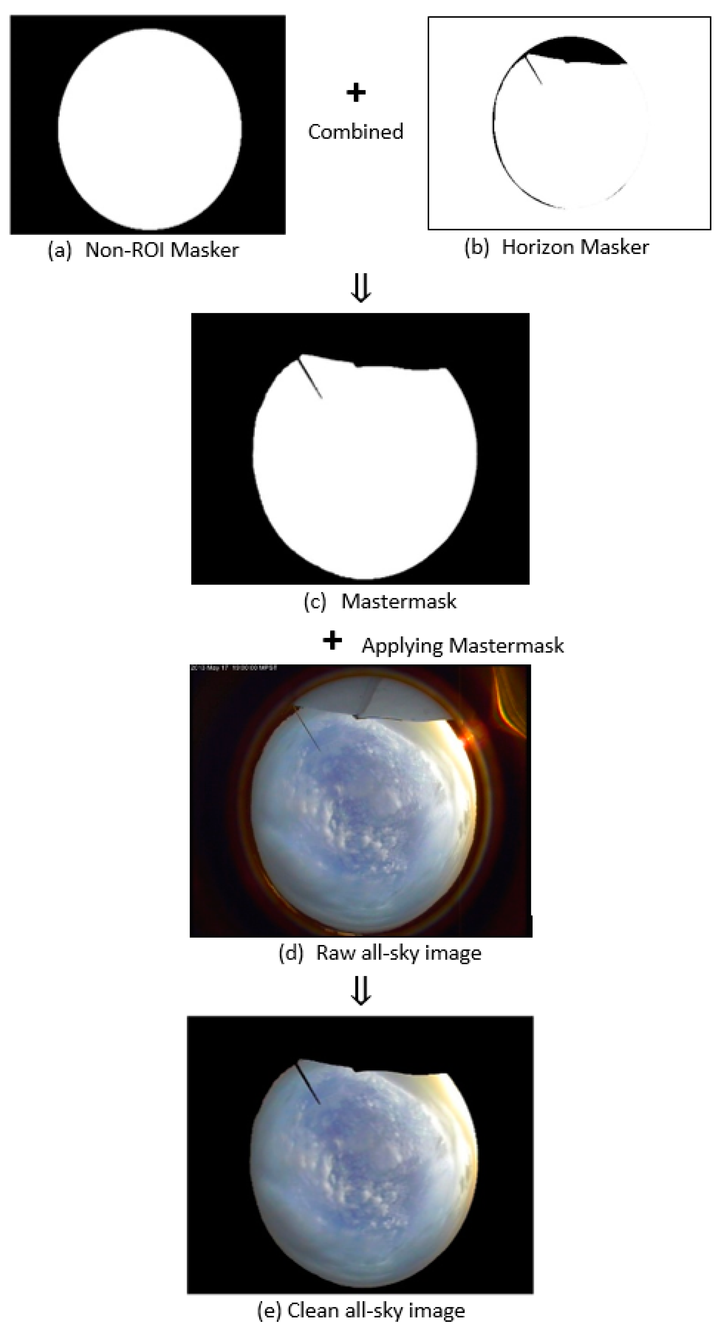
Generally, masking is a method of obscuring certain undesirable regions, thus allowing us to deal only with the pixels inside the region of interest (ROI) chosen. In our study, the mask was actually a binary image of the same size as the raw all-sky image, which is 570 × 720 pixels. Basically, two stages of masking were involved in this study. The first stage involved creating basic masks for each type of unnecessary pixels. For this stage, two basic masks were created based on the problem discovered on the raw images. The first basic mask is called the Non-ROI mask, which masked the whole image except for the ROI part. The mask eliminated all pixel values caused by the sunlight reflected outside of the ROI. The second mask is the Horizon mask that handled the pixels that did not represent the sky region within the ROI. In this stage, a pixel value of ‘one’ represented the ROI while a pixel value of ‘zero’ represented the Non-ROI and horizon objects. The second stage involved producing a mastermask by combining both the Non-ROI and Horizon mask into one mask. The mastermask was then applied onto the raw all-sky image to produce a clean image.
We applied the mastermask by multiplying the mask with the raw image. Since the ROI pixel value was multiplied by one, the value remained the same. In contrast, the rest became zero after they were multiplied by zero. As a result, we were able to obtain pixel values only from the pixels inside the ROI since pixels in the Non-ROI had a pixel value of zero.
4. Cloud Detection Method
The cloud detection method used in this study is based on the Color Difference method. Instead of using the conventional way of R-B Color Difference, we explored a different way of cloud detection using B-G Color Difference. The cloud detection method can be divided into two main stages, which are the threshold determination and the cloud coverage stage.
4.1. All-Sky Images
A total of 15 all-sky images were chosen, which consist of five images of each sky conditions (clear, partially cloudy and overcast) within the range of May 2013 to May 2016. All of the images have to go through the pre-processing phase before thresholding or cloud coverage measurement are implemented on the images.
4.2. Threshold
In order to obtain the B-G threshold value, we compared pixel values from 30 raw all-sky images. For each all-sky image, ten pixels that were randomly chosen from the sky regions. The pixel value of each red, green and blue color channel is extracted for each pixel. The difference value between a pixel value of blue and red color channel is calculated for each of the randomly selected pixels. The threshold value was then estimated based on the average of all of the difference values for all of the selected pixels.
In this study, we had to obtain the R-B threshold value for comparison purposes. The method is the same as the B-G threshold value. However, in order to simplify the calculation, we calculate the R-B Color Difference by subtracting the blue pixel value with the red pixel value, in order to simplify the calculation and algorithm.
4.3. Cloud Coverage
By using the B-G threshold value, we were able to determine what each of the pixels represented. Basically, if a pixel has a B-G value higher than the threshold value, then the pixel is a sky-pixel. Cloud coverage can be represented by the Cloud Coverage Ratio (CCR) using Equation (1):
where Ncloud is the number of cloud-pixels and Nsky is the number of sky-pixels.
5. Result and Discussion
Based on the comparison study of B-G values between sky-pixel and cloud-pixel done in previous studies, we chose B-G = 30 as the threshold value for the current study [22]. Any pixel with a B-G pixel value higher than 30 was therefore considered a sky-pixel whereas pixels with lower values were considered a cloud-pixel. We also used the same method to determine the threshold value for R-B and the value was also 30. The value is acceptable since it is within the optimal range as stated by Heinle et al. [18]. This value is necessary in carrying out the comparison between B-G and R-B since the threshold value can be different depending on the location.
Figure 5 shows the comparison between R-B and B-G Color Difference for clear, partially cloudy and overcast sky conditions. Overall, both methods of Color Difference can detect the thick clouds as seen in the images of the partially cloudy and overcast sky condition. However, the new method of B-G Color Difference seems to detect the thin high-cloud better than R-B Color Difference. There were a number of pixels or regions in the clear and partially cloudy sky condition images where R-B Color Difference considered them as sky pixels even though there was a thin layer of cloud. As for B-G Color Difference, the thin layer of cloud was detected clearly. The ability to detect even a thin cloud layer is crucial in astronomical observations. This is because a thin layer of cloud can severely affect the outcome of observations such as photometry, especially when doing long exposure imaging.
In terms of cloud coverage percentage, most of the results of B-G Color Difference gave higher percentages of cloud-covered sky. This can be seen in the cloud coverage percentage comparison between B-G and R-B Color Difference presented in Table 2. The percentage differences between them are 25.76%, 20.92% and 0.02% for clear, partially cloudy and overcast sky conditions, respectively. The percentage difference for clear and partially cloudy sky conditions shows a very large gap in cloud-pixel counts between both methods because of the thin cloud detection. These results indicate the ability of the B-G Color Difference method in detecting both thick and thin clouds, which thus increases the detection of cloud-pixels significantly. On the other hand, the significant percentage differences indicate the failure of R-B Color Difference in detecting thinner clouds. As for the overcast sky condition, we found that both methods were able to detect them perfectly with a very low percentage difference between the two readings.
In order to further check the effectiveness of B-G Color Difference in detecting thin clouds, we compared the cloud detection of both methods using cropped all-sky images of a clear blue sky and a thin cloudy region. The cloud coverage percentages are as shown in Table 3. For the clear sky cropped image, both methods show zero percent cloud coverage. However, for the thin clouds cropped images, the B-G method was able to detect more thin clouds compared to the R-B method, as shown in Table 3.
There is one problem that needs to be highlighted in this study, which is the lack of solar obscuration over the all-sky imager to block the direct and blinding sunlight. Without the solar obscuration, a blooming effect will occur in the image, especially when taking images under clear sky conditions. Figure 6a shows an example of such effect while Figure 6b shows the solar obscuration blocking the glaring sunlight. It was very difficult to identify the pixels of the overflowing limb from the blooming effect since the Color Difference was mostly approaching zero, and thus would be considered cloud-pixels. The all-sky imager installed at PERMATApintar Observatory is not equipped with a solar obscuration as the system is not meant for the purpose of this study. One possible solution for the problem is by introducing another criterion of pixel characterization, which is the average R, G and B channel of a pixel. Theoretically, a thick cloud should have a darker gray color as it absorbs the sunlight, thus resulting in a lower average value. However, we must consider other conditions that have almost the same attribute as the blooming effect. Some examples of the conditions are the bright white side of cumulus clouds due to sunlight reflection and bright light scattering by cirrus or cirrostratus clouds during sunrise, which is also known as the whitening effect. Hence, future study is needed to differentiate and characterize the pixels in order to increase the effectiveness of this type of cloud detection method.
6. Conclusions
In this study, we have developed a cloud detection method that is able to detect cloud effectively based on the Color Difference approach, called the B-G Color Difference method. The effectiveness of the B-G Color Difference method has been proven through the comparison carried out with the commonly used R-B Color Difference method. We have reported that the threshold value for both B-G and R-B is 30 where sky-pixels are represented by values higher than the threshold and vice versa. Our study revealed the better ability of the B-G method in detecting more cloud coverage especially in clear and partially cloudy sky conditions compared to the R-B method. This is mainly due to the ability of the B-G method to detect thin clouds better than the R-B method. The percentage difference of cloud coverage readings between these two methods for clear, partially cloudy and overcast sky conditions is 25.76%, 20.92% and 0.02%, respectively. Further analysis carried out in terms of thin clouds detection using cropped images of clear and thin cloud region has shown that that B-G method can detect thin cloud better than the R-B method.
Author Contributions
Original draft preparation: M.A.D.M.A., N.S.A.H. and W.M.A.W.M.K.; figures: M.A.D.M.A. and N.S.A.H.; draft review and revise: N.S.A.H., W.M.A.W.M.K. and N.S.M. All authors have read and agreed to the published version of the manuscript.
Funding
The APC was funded by GENIUS@Pintar National Gifted Centre through the allocation of PERMATA-2015-001 (AKU67).
Institutional Review Board Statement
Not applicable.
Informed Consent Statement
Not applicable.
Data Availability Statement
Data sharing not applicable.
Acknowledgments
The authors would like to express their gratitude to the Ministry of Higher Education of Malaysia for the MyPhD scholarship and GENIUS@Pintar National Gifted Centre for funding the APC for this article.
Conflicts of Interest
The authors declare no conflict of interest.
References
- Graham, E. A Site Selection Tool for Large Telescopes Using Climate Data. Ph.D. Thesis, University of Bern, Bern, Switzerland, 2008; p. 153. [Google Scholar]
- Carrasco, E.; Carramiñana, A.; Sánchez, L.J.; Avila, R.; Cruz-González, I. An estimate of the temporal fraction of cloud cover at San Pedro Mártir Observatory. Mon. Not. R. Astron. Soc. 2012, 420, 1273–1280. [Google Scholar] [CrossRef] [Green Version]
- Graham, E.; Vaughan, R.; Buckley, D. Search for an Astronomical Site in Kenya (SASKYA) update: Installation of on-site automatic meteorological stations. J. Phys. Conf. Ser. 2015, 595, 012012. [Google Scholar] [CrossRef]
- Cole, F.W. Introduction to Meteorology, 3rd ed.; John Wiley & Son: New York, NY, USA, 1980; p. 505. [Google Scholar]
- Azhari, A.W.; Sopian, K.; Zaharim, A.; Al Ghoul, M. A new approach for predicting solar radiation in tropical environment using satellite images-case study of Malaysia. WSEAS Trans. Environ. Dev. 2008, 4, 373–378. [Google Scholar]
- Azhari, A.W.; Sopian, K.; Zaharim, A.; Al Ghoul, M. Solar radiation maps from satellite data for a tropical environment: Case study of Malaysia. In Proceedings of the 3rd IASME/WSEAS International Conference on Energy & Environment, Cambridge, UK, 23–25 February 2008; pp. 528–533. [Google Scholar]
- Shavalipour, A.; Hakemzadeh, M.H.; Sopian, K.; Mohamed Haris, S.; Zaidi, S.H. New formulation for the estimation of monthly average daily solar irradiation for the tropics: A case study of Peninsular Malaysia. Int. J. Photoenergy 2013, 2013, 174671. [Google Scholar] [CrossRef]
- Badescu, V.; Dumitrescu, A. CMSAF products Cloud Fraction Coverage and Cloud Type used for solar global irradiance estimation. Meteorol. Atmos. Phys. 2016, 128, 525–535. [Google Scholar] [CrossRef]
- Khatib, T.; Mohamed, A.; Mahmoud, M.; Sopian, K. An assessment of diffuse solar energy models in terms of estimation accuracy. Energy Procedia 2012, 14, 2066–2074. [Google Scholar] [CrossRef] [Green Version]
- Radu, A.A.; Angelescu, T.; Curtef, V.; Felea, D.; Hasegan, D.; Lucaschi, B.; Manea, A.; Popa, V.; Ralita, I. An astroclimatological study of candidate sites to host an imaging atmospheric Cherenkov telescope in Romania. Mon. Not. R. Astron. Soc. 2012, 422, 2262–2273. [Google Scholar] [CrossRef] [Green Version]
- Smith, A.W. Multiwavelength Observations of the TeV Binary LS I+ 61303. Ph.D. Thesis, University of Leeds, Leeds, UK, 2007. [Google Scholar]
- Koehler, T.L.; Johnson, R.W.; Shields, J.E. Status of the whole sky imager database. In Proceedings of the Cloud Impacts on DOD Operations and Systems, 1991 Conference, El Segundo, CA, USA, 1 December 1990; pp. 77–80. [Google Scholar]
- Huo, J.; Lu, D. Cloud determination of all-sky images under low-visibility conditions. J. Atmos. Ocean. Technol 2009, 26, 2172–2181. [Google Scholar] [CrossRef]
- Zain-Ahmed, A.; Sopian, K.; Abidin, Z.Z.; Othman, M.Y.H. The availability of daylight from tropical skies—a case study of Malaysia. Renew. Energy 2002, 25, 21–30. [Google Scholar] [CrossRef]
- Kazantzidis, A.; Tzoumanikas, P.; Bais, A.F.; Fotopoulos, S.; Economou, G. Cloud detection and classification with the use of whole-sky ground-based images. Atmos. Res. 2012, 113, 80–88. [Google Scholar] [CrossRef]
- Ghonima, M.S.; Urquhart, B.; Chow, C.W.; Shields, J.E.; Cazorla, A.; Kleissl, J. A method for cloud detection and opacity classification based on ground based sky imagery. Atmos. Meas. Tech. 2012, 5, 2881–2892. [Google Scholar] [CrossRef] [Green Version]
- Silva, A.A.; de Souza Echer, M.P. Ground-based measurements of local cloud cover. Meteorol. Atmos. Phys. 2013, 120, 201–212. [Google Scholar] [CrossRef]
- Heinle, A.; Macke, A.; Srivastav, A. Automatic cloud classification of whole sky images. Atmos. Meas. Tech. 2010, 3, 557–567. [Google Scholar] [CrossRef] [Green Version]
- Yang, J.; Min, Q.; Lu, W.; Yao, W.; Ma, Y.; Du, J.; Lu, T.; Liu, G. An automated cloud detection method based on the green channel of total-sky visible images. Atmos. Meas. Tech. 2015, 8, 4671–4679. [Google Scholar] [CrossRef] [Green Version]
- Liu, S.; Zhang, L.; Zhang, Z.; Wang, C.; Xiao, B. Automatic Cloud Detection for All-Sky Images Using Superpixel Segmentation. IEEE Geosci. Remote Sens. Lett. 2015, 12, 354–358. [Google Scholar] [CrossRef]
- Moonglow Technologies: All Sky Cam: All Sky Cam Uploader for Windows. Available online: http://www.moonglowtech.com/products/AllSkyCam/Software.shtml (accessed on 5 February 2019).
- Azhar, M.A.; Hamid, N.S.; Kamil, W.M.; Mohamad, N.S. Urban Night Sky Conditions Determination Method Based on a Low Resolution All-Sky Images. In Proceedings of the 2019 6th International Conference on Space Science and Communication (IconSpace), Johor Bahru, Malaysia, 28–30 July 2019; pp. 158–162. [Google Scholar]
Figure 1.
(a) An image of the PERMATApintar Observatory and (b) an enlarged image of the all-sky imager next to the observatory.
Figure 1.
(a) An image of the PERMATApintar Observatory and (b) an enlarged image of the all-sky imager next to the observatory.

Figure 2.
A snapshot of the ASC Uploader [21].
Figure 2.
A snapshot of the ASC Uploader [21].

Figure 3.
A raw all-sky image taken by the all-sky imager at PERMATApintar Observatory (a). The following three images are the red (b), green (c) and blue (d) color channels split of the raw all-sky image.
Figure 3.
A raw all-sky image taken by the all-sky imager at PERMATApintar Observatory (a). The following three images are the red (b), green (c) and blue (d) color channels split of the raw all-sky image.

Figure 4.
The figure shows the masking process. The mastermask (c) is produced by combining the Non-ROI (a) with the Horizon masker (b). The mastermask is then applied to the raw all-sky image (d) to obtain the clean all-sky image (e).
Figure 4.
The figure shows the masking process. The mastermask (c) is produced by combining the Non-ROI (a) with the Horizon masker (b). The mastermask is then applied to the raw all-sky image (d) to obtain the clean all-sky image (e).

Figure 5.
(a) The all-sky images of three sky conditions (clear, partially cloudy and overcast) while their R-B and B-G Color Difference outcomes are shown in (b,c), respectively.
Figure 5.
(a) The all-sky images of three sky conditions (clear, partially cloudy and overcast) while their R-B and B-G Color Difference outcomes are shown in (b,c), respectively.

Figure 6.
(a) An all-sky image taken from PERMATApintar Observatory during a clear sky with a blooming effect. (b) An example of solar obscuration that blocks the Sun (Radu et al. 2012) [10].
Figure 6.
(a) An all-sky image taken from PERMATApintar Observatory during a clear sky with a blooming effect. (b) An example of solar obscuration that blocks the Sun (Radu et al. 2012) [10].


Table 1.
The specifications of the all-sky imager [21].
Table 1.
The specifications of the all-sky imager [21].
| Characteristics | Specifications |
|---|---|
| Image sensor | Color 1/3” Sony Super HAD CCD II |
| Lens | 1.24 mm, F2.8 |
| Field of view | 190 degrees hemispherical |
| Imaging rate | 1/100,000 s to 4 s (automatic) |
| Weight | 0.3 kg |
| Data storage | Connected to a computer |
Table 2.
Cloud Coverage Percentage for both Color Difference in three different sky conditions.
| Sky Conditions | Cloud Coverage Percentage (%) | Percentage Difference (%) | |
|---|---|---|---|
| R-B | B-G | ||
| Clear | 31.11 | 40.31 | 25.76 |
| Partially Cloud | 73.98 | 91.26 | 20.92 |
| Overcast | 99.98 | 100.00 | 0.02 |
Table 3.
Thin cloud detection and coverage percentage for B-G and R-B Color Difference.
| Sky Conditions | Cloud Coverage Percentages | |
|---|---|---|
| R-B | B-G | |
| Clear sky | ||
 |  |  |
| 0% | 0% | |
| Partially cloudy | ||
 |  |  |
| 16.53% | 37.52% | |
Publisher’s Note: MDPI stays neutral with regard to jurisdictional claims in published maps and institutional affiliations. |
© 2021 by the authors. Licensee MDPI, Basel, Switzerland. This article is an open access article distributed under the terms and conditions of the Creative Commons Attribution (CC BY) license (http://creativecommons.org/licenses/by/4.0/).
Share and Cite
MDPI and ACS Style
Azhar, M.A.D.M.; Hamid, N.S.A.; Kamil, W.M.A.W.M.; Mohamad, N.S. Daytime Cloud Detection Method Using the All-Sky Imager over PERMATApintar Observatory. Universe 2021, 7, 41. https://0-doi-org.brum.beds.ac.uk/10.3390/universe7020041
AMA Style
Azhar MADM, Hamid NSA, Kamil WMAWM, Mohamad NS. Daytime Cloud Detection Method Using the All-Sky Imager over PERMATApintar Observatory. Universe. 2021; 7(2):41. https://0-doi-org.brum.beds.ac.uk/10.3390/universe7020041
Chicago/Turabian StyleAzhar, Mohammad Afiq Dzuan Mohd, Nurul Shazana Abdul Hamid, Wan Mohd Aimran Wan Mohd Kamil, and Nor Sakinah Mohamad. 2021. "Daytime Cloud Detection Method Using the All-Sky Imager over PERMATApintar Observatory" Universe 7, no. 2: 41. https://0-doi-org.brum.beds.ac.uk/10.3390/universe7020041
Note that from the first issue of 2016, this journal uses article numbers instead of page numbers. See further details here.