
Mechanisms and Evolution of Geoeffective Large-Scale Plasma Jets in the Magnetosheath


1
Department of Space Science & Engineering, National Central University, 300 Zhongda Road, Zhongli, Taoyuan City 320, Taiwan
2
Skobeltsyn Institute of Nuclear Physics, Lomonosov Moscow State University, 11991 Moscow, Russia
3
Graduate Institute of Astronomy, National Central University, 300 Zhongda Road, Zhongli, Taoyuan City 320, Taiwan
4
Intelligent Datanalytics, Zhongyang Road, Pingzhen District, Taoyuan City 324, Taiwan
*
Author to whom correspondence should be addressed.
Universe 2021, 7(5), 152; https://0-doi-org.brum.beds.ac.uk/10.3390/universe7050152
Submission received: 3 April 2021
/
Revised: 30 April 2021
/
Accepted: 7 May 2021
/
Published: 17 May 2021
(This article belongs to the Special Issue Space Weather)
Abstract
:Geoeffective magnetosheath plasma jets (those that interact with the magnetopause) are an important area of research and technology, since they affect the “space-weather” around the Earth. We identified such large-scale magnetosheath plasma jets with a duration of >30 s using plasma and magnetic data acquired from the Time History of Events and Macroscale Interactions during Substorms (THEMIS) multi-spacecraft experiment during the years 2007 to 2009. We present a statistical survey of 554 of such geoeffective jets and elaborate on four mechanisms for the generation of these jets as the upstream solar wind structures of tangential discontinuities (TDs), rotational discontinuities (RDs), the quasi-radial interplanetary magnetic field (rIMF) and the collapsing foreshock (CFS) interrupting the rIMF intervals. We found that 69% of the jets are generated due to the interaction between interplanetary discontinuities (TD: 24%, RD: 25%, CFS: 20%) with the bow shock. Slow and weak jets due to the rIMF contributed to 31% of these jets. The CFS and rIMF were found to be similar in their characteristics. TDs and RDs contributed to most of the fast and powerful jets, with large spatial scales, which might be attributed to transient effects in the travelling foreshock.
Keywords:
space weather; interplanetary discontinuities; geoeffectiveness; magnetosheath plasma jetsPACS:
47.27.Wg; 94.05.Sd; 94.30.cq; 94.30.cv; 92.60.hx1. Introduction
The terrestrial magnetic field presents a potent deterrent to the interplanetary magnetic fields (IMFs) and magnetised particles emanating from solar processes [1]. This causes various interactions in the region where the magnetized solar plasma interacts with the Earth’s magnetic field, namely the bow shock and the magnetosphere (see Figure 1 of [2] for a visual description). A highly complex and non-linear interaction that ensues in this region has been the subject of rigorous study in the past few decades. In particular, the deceleration of the solar wind at the bow shock causes significant transient flux enhancements, which are also known as magnetosheath plasma jets [2,3]. These jets can interact with the magnetopause, the magnetic boundary shielding the Earth, which makes them geoeffective, that is they can cause disruptive events on either the Earth or in the space near the Earth [2,4,5].
The mechanism of the origin of these jets is a hotly contested topic in the space weather community due to the various methods of identification and classification of these phenomena. This requires a reliable and accurate model for the mechanism of jet generation in the magnetosphere. Various generation mechanisms for jets have been proposed and analysed in recent years: the interaction of interplanetary discontinuities [6] with the foreshock and bow shock [7], hot flow anomalies [8,9] generated through the interaction of tangential discontinuities (TDs) with the quasi-parallel element of the bow shock and interactions between the bow shock and a rotational discontinuity (RD) [10,11,12].
In this article, we analysed four mechanisms of magnetosheath jet generation and their evolution. In contrast to the existing theories, we showed that jets might not always be well developed at the outer regions of the magnetosheath, but develop deeper and closer to the magnetopause. We also present case studies, where the jets might be swept away by the turbulent magnetospheric plasma dynamics. We present a statistical analysis of these four types of jets with observations on the geoeffectiveness of the magnetosheath jets.
Magnetospheric jets can be characterised distinctively as energy enhancements in short periods of time (of the order of ×10 s) in a very localised region, where these enhancements of energy exceed that of the upstream solar wind. There are different mechanisms that have been variously attributed to generating these jets. The four kinds of jet origins are via the interactions of
- collapsing foreshock (CFS) [19]
Briefly, the discontinuities as mentioned in Points 1 and 2 are collectively called directional discontinuities and are shown to generate jets, pushing the magnetopause locally and causing prominent geomagnetic variations [8,9,20,21,22].
Condition 3 can cause multiple short-duration jets [17], and as shown in [18], they are formed for the cone angle < 30° (see Section 2.3 and [23,24] for the definition of ). Savin et al. [25] suggested that under rIMF conditions, a non-fully developed turbulence in the magnetosheath can form a jet (also see [9]). More specifically, as observed by Lin et al. [10], Tsubouchi and Matsumoto [11], Dmitriev and Suvorova [12], an interaction between the RD and bow shock can cause an increase in magnetosheath plasma pressure via deflection and focusing of the downstream plasma flow, and thus can lead to a magnetosheath jet. In addition, a pressure pulse is formed in the foreshock region when a sector of the quasi-parallel bow shock is converted into a quasi-perpendicular one [10]. This accelerating upstream pressure pulse that impacts the downstream pulse can enforce the jet [11,18], and this enforced jet can propagate across the streamlines to interact with the magnetopause, thereby making it geoeffective [18].
Further mechanisms based on the formation of ripples in the quasi-parallel bow shock [26] have also been proposed, augmented by the observations of Lucek et al. [27] that large-scale foreshock fluctuations steepen as they propagate towards the Earth, dynamically forming and reforming the shock ramp, signifying that the quasi-parallel shock is inherently rippled (although Archer and Horbury [28] challenged this idea). Nevertheless, the rIMF mechanism is found to be responsible for only ∼10–15% of the jets observed [17,29].
Dmitriev and Suvorova [12,18] exposited that large-scale jets with a duration longer than 30 s interact effectively with the magnetopause, with the jet duration peaking approximately at 30 s [24,28], thus motivating the definition of “large-scale” jets to be longer than 30 s in duration. This can result in a significant amount of penetration of the magnetosheath plasma inside the day-side magnetosphere, thus causing these large-scale plasma jets to compete with the magnetic reconnection effect at the day-side magnetopause. Thus, an investigation of the different mechanisms of jet origins, their evolution through the magnetosheath and their geoeffectiveness (interaction, if any, with the magnetopause) is warranted. The present study focused on geoeffective large-scale jets, which interact with the magnetopause and produce geomagnetic pulses. We continued the previous work by Dmitriev and Suvorova [18]: we analysed carefully the upstream solar wind conditions in order to investigate the mechanism of origin and evolution of the jets.
The article is organised as follows: Section 2 contains a summary of the data used (Section 2.1), the definitions of geoeffective jets (Section 2.2) and the identification of interplanetary sources responsible for the jet origins (Section 2.3). We discuss case studies of the four identified jet mechanisms in Section 3, with tangential discontinuities in Section 3.1, rotational discontinuities in Section 3.2, quasi-radial IMF in Section 3.3 and collapsing foreshocks in Section 3.4. We further perform a statistical analysis of the observed jets during 2007–2009 in Section 3.5. We present a discussion of the results in this article in Section 4 and follow with a conclusion.
2. Methods
2.1. Data
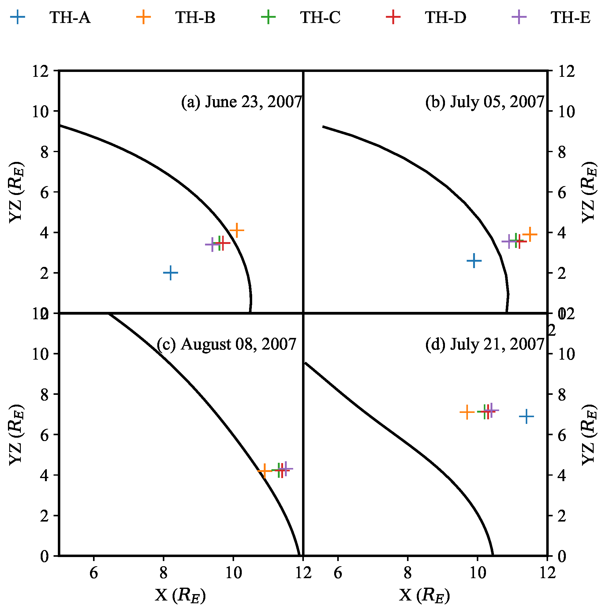
We used the THEMIS multi-spacecraft experiment [30] in the magnetosheath (magnetosheath) and the ACE [31] and WIND [32] monitors located far upstream (∼230 ) in the solar wind (solar wind) with a time resolution of ∼16 s (see [18] for details). The magnetic field and plasma were measured at different THEMIS spacecraft locations with a time resolution of ∼3 s by the Flux Gate Magnetometer (FGM) [33] and the Electrostatic Analyser (ESA) operating in a fast survey mode [34]. The THEMIS probes are arranged in a “string-of-pearls” configuration around the bow shock and in the magnetosheath. We determined the positions of the bow shock from Chao et al. [35] and magnetopause based on Lin et al. [36] in this study (see Dmitriev et al. [37] for a comparison of the models). The THEMIS spacecraft positions with respect to the magnetopause are shown in Figure 1 for the four demonstrative cases discussed in Section 3. All vector parameters in this study are presented in Geocentric Solar Magnetospheric (GSM) coordinates (unless stated otherwise).
In contrast to the CLUSTER [38] and MMS [39] missions, THEMIS provides a unique opportunity to observe large-scale plasma structures simultaneously in a spatial scale of several Earth radii () corresponding to a significant spatial regime of the interaction region (the magnetosheath in the present case) [30].
2.2. Identification of Geoeffective Plasma Jets in the Magnetosheath
Dmitriev and Suvorova [18] defined a large-scale jet as a magnetosheath plasma structure, whose total energy ratio for >30 s; with and being the total energy densities measured, respectively, by THEMIS in the magnetosheath and by the upstream monitors in the solar wind. The total energy density (or pressure) can be obtained as a sum of the kinetic , thermal and magnetic pressures:
where are the densities of the proton, electron and helium (in cm−3), respectively; are respectively the electron and proton temperatures (in K), plasma velocity V in km/s and the magnetic field (in nT). , , , respectively, are the coefficients necessary while converting units from one system to another. The pressure P is in units of nPa and holds for both upstream and downstream conditions. The high kinetic energy ratio , where is measured within the magnetosheath, is indicative of high-speed jets [12,18].
The set of the large-scale jets collected by Dmitriev and Suvorova [18] from 2007–2009 was used in this article. Being in a “string-of-pearls” positional configuration, the evolution of a single jet in the magnetosheath can be tracked by the THEMIS constellation. The jet characteristics are determined for the probes, which detect the highest , which is usually observed in the middle magnetosheath. This can be attributed to the fact that the jet may not be well developed in the outer magnetosheath and can decelerate as it approaches the magnetopause [18]. The jets identified in this study were localised to 80° longitude to minimise the effects at the flanks such as Kelvin–Helmholtz waves at the magnetopause flank and tail [40]. Consequently, a set of 646 large-scale jets was collected in the pre-noon, noon, and post-noon sectors at latitudes from −35° to 10°.
The interaction of the jet with the magnetopause was analysed by converting the coordinates into a new set of coordinates ) following Dmitriev et al. [37], in the frame of the reference magnetopause calculated for given upstream solar wind conditions. Here, is in the magnetopause plane and points northwards and is the magnetopause normal that points outwards, and completes the triad by pointing downward.
We used the magnetopause model by Lin et al. [36] for the prediction of the dayside magnetopause in the widest dynamic range of upstream conditions [18,41]. We showed that a jet with a large negative normal component of of velocity of the range of hundreds of km/s can impact the magnetopause [42], implying that the geoeffective jets should have a high speed and thus a large contribution of in [18].
The interaction of a jet with the magnetopause results in a local transient compression [12]. This compression, in the magnetosphere, causes a magnetic pulse at low to mid-latitudes and/or travelling convection vortices at high latitudes [12,23]. The magnetic pulse can be found in magnetic data acquired from the inner-most THEMIS probes located in the magnetosphere, or from the GOES geosynchronous satellite, or even as an increase of the 1 min SYM-H index measured by ground-based magnetic stations at low latitudes. In contrast to other geomagnetic indices, the SYM-H index is sensitive to variations of the magnetopause surface current, which is directly affected by jets [43].
Interaction of a jet with the magnetopause can result in the deflection of the fast plasma flow into the sunward direction [12,18,44], thereby causing magnetosheath plasma streams with due to the deflection effect [45], and thus should not be considered to be a constitutive part of a geoeffective plasma jet, which should have an anti-sunward direction. Therefore, the definition of large-scale geoeffective plasma jets can be formulated as the following: they should have both and for or longer. The original set of 646 large-scale jets was thus revised according to these definitions.
2.3. Identification of Interplanetary Sources
We distinguished four kinds of upstream solar wind structures, which can contribute to the formation of magnetosheath plasma jets: tangential discontinuities (TDs) [14], rotational discontinuities (RDs) [6,46,47], quasi-radial IMF (rIMF) [17,48], and CFS [12]. Both TDs and RDs are directional discontinuities. Following Neugebauer et al. [13], we defined a discontinuity as a structure, across which the IMF rotates and may change its magnitude. TDs were defined to have no magnetic component normal to the magnetic field rotation plane: [13]. They are characterised by a large change of magnetic field such that and constant plasma velocity across the discontinuity [12].
Rotational discontinuities [47] have non-zero , and they are characterised by a small change of the magnetic field , but a large change of the transversal plasma velocity ( > 10 km/s) across the discontinuity [18]. Note that is calculated as the difference of the magnetic field before and after (thus, across) a discontinuity, with the time scale in minutes. RDs propagate in the solar wind frame along the normal with and Alfvén velocity determined by the . A Walén test [49] can be used to verify the nature of a discontinuity. However, the low temporal resolution of the upstream plasma data made it difficult to perform the test accurately.
The structure of a rIMF is defined in the solar wind as a plasma stream with IMF orientation almost aligned with the stream [12]; that is, a cone angle (in degrees); the angle between the plasma velocity and IMF vector should be small, that is, < 30° for more than 10 min. The later additional criterion is required for the complete formation of a foreshock in the subsolar region [12,18,41]. rIMF structures are accompanied by strong fluctuations in the magnetic field and by the appearance of accelerated ions with energies above several keV (see for example [50,51,52,53]).
A CFS occurs at the end of rIMF intervals. It is produced by a discontinuity, across which the increases abruptly and exceeds the threshold of 20°, which results in the collapse of the foreshock in the subsolar region [12,18]. The collapse is accompanied by very fast non-equilibrium dynamic processes such as the generation of plasma jets and the very fast anti-sunward motion of the bow shock and magnetopause [54]. Thus, we expected that CFS structures could result in the generation of very strong geoeffective jets.
3. Results
We present our results by first elaborating on case studies based on the four interplanetary sources described above, namely tangential discontinuity (Section 3.1), rotational discontinuity (Section 3.2), quasi-radial IMF (Section 3.3), and collapsing foreshock (Section 3.4). Following a detailed discussion of the various jets observed under these mechanisms, we give a statistical analysis of the observed discontinuities and their role in generating geoeffective jets in Section 3.5.
3.1. Tangential Discontinuity
A tangential discontinuity is characterised by and . Owing to the locations of the THEMIS probes (refer to the position panel in Figure 2, with TH-A, TH-B, TH-C, TH-D and TH-E probes located respectively at , , , , and .
The TH-C detected the prominent Jets 1 and 2 deep in the magnetosheath (see Panels (c) and (d) of Figure 2). These two jets are separated by an interval of small or even positive . The intervals where before and after the jets characterised by and are observed can be related to plasma streams deflected by the magnetopause during interactions with the jets [12].
The more prominent Jet 2 characterised by with an indicates a large contribution to the jet with a velocity of ∼230 km/s (Figure 2d) and ≈ −145 km/s as observed by TH-B (Figure 2b). Jet 1 also proceeded with ≈ −125 km/s towards the magnetopause. Deeper in the magnetosheath, from 06:22:30 UT to 06:23:40 UT, the jets were observed by TH-D and TH-E through the ion spectra (Figure 2k–o) in logarithmic scales, as a prominent increase in the differential ion fluxes of the order of 1 keV, while in the magnetosheath, these fluxes might vary from ∼103–108 cm3 s sr eV−1).
Figure 2 shows that the jets move towards the Earth, impact the magnetosphere and result in a local compression of the magnetopause, which was observed by the innermost TH-A probe as an increase in the magnetic field strength by more than 10 nT in the time interval between 06:21 UT and 06:27 UT (see Figure 2p). This increase is caused by the approach of electric current at the magnetopause at the probe. Note that the duration of compression is wider than the time intervals in which the jets were observed by the THEMIS probes. This might be explained by the effect of travelling magnetopause distortions associated with the development of large-scale plasma jets [12,55]. Thus, we showed that a jet can be substantially extended in space, and it is a dynamic structure, that is it can develop in a time span of minutes in both radial and transversal directions. As a result, the time of detection and impact time of the jet depend strongly on the observation point an can vary by several minutes.
A directional discontinuity was observed by the ACE upstream monitor between 05:43 UT and 05:45 UT (about half an hour before the observation of the jet), while being situated at . The corresponding solar wind and IMF conditions are presented in Figure 2e–h with a 40 min time delay (clarified later). The discontinuity can be found around 06:23 UT and is formed by abrupt and large changes in the and IMF components, with a corresponding increase in the magnetic field from 3.43 nT to 4.09 nT such that . These features effectively suggest the directional discontinuity to be a tangential discontinuity.
The normal to the TD can be calculated using minimum variance analysis (MVA) [56]. Briefly, MVA allows finding, from single-spacecraft data, eigenvectors and their eigenvalues (, , ) in the frame of specific coordinates associated with a plasma transition layer, such as directional discontinuity. The method was applied for the time interval from 05:43 UT to 05:45 UT and gave a normal to the rotation plane, = (−0.98, 0.19, 0.07) and eigenvalues . We observed that , which corresponds to a tangential discontinuity [12].
Taking into account the ACE location and the vector of the solar wind velocity, we calculated the propagation time of TD from ACE to a given point: = 39 min for the subsolar bow shock with coordinates (14, 0, 0); and = 40 min the propagation time to the TH-B position (10.1, 2.9, −2.9). Note that the propagation time can be determined with a few minutes of uncertainty because of the possible change in the orientation of the interplanetary fronts during the propagation of a large distance from ACE [57]. As mentioned in Section 2.3, a TD is considered as a source of a hot flow anomaly, which can result in the generation of a pair of jets. Hence, we suggest that in the present case, the jets originate from a tangential discontinuity.
3.2. Rotational Discontinuity
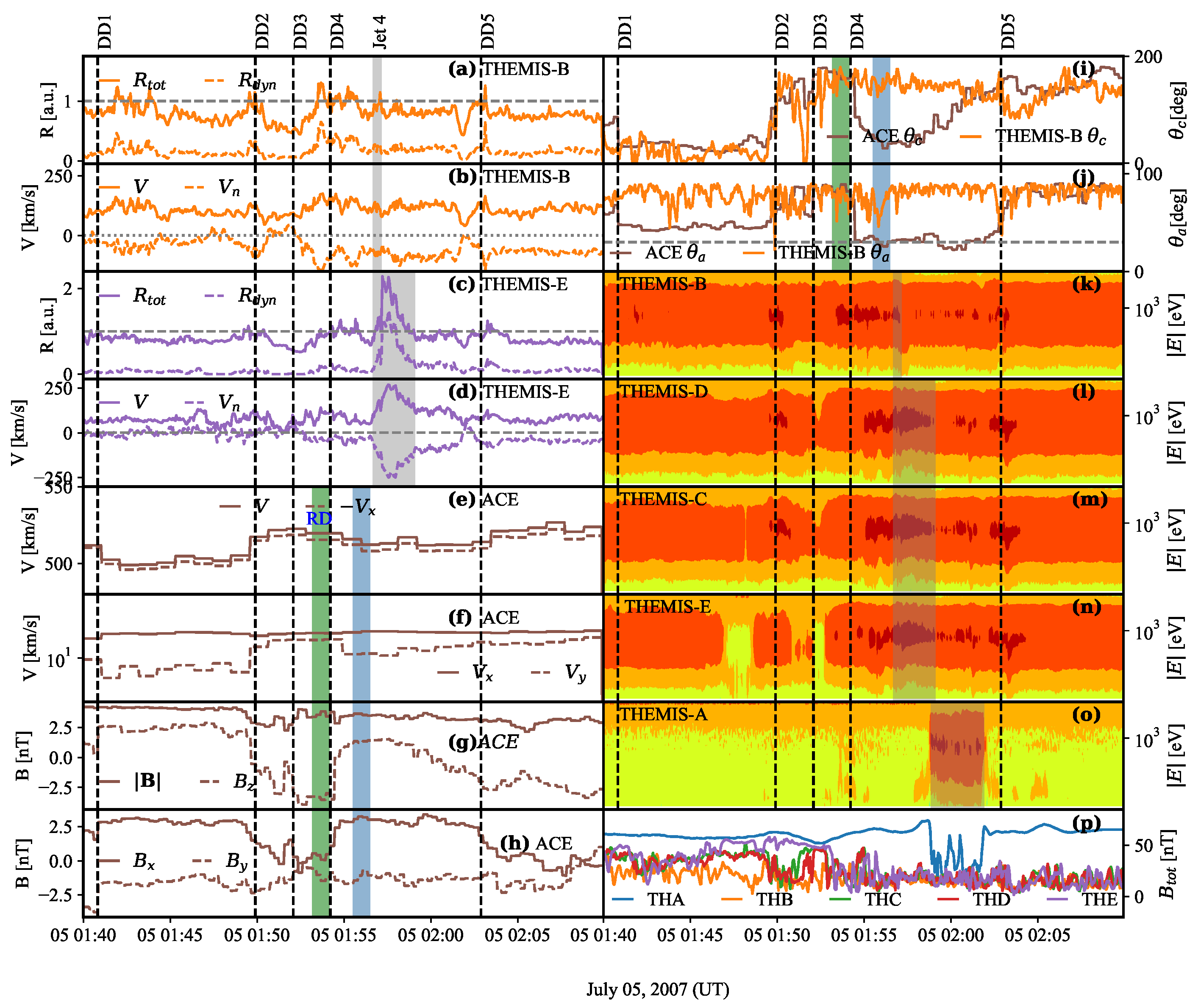
A comprehensive analysis of a large-scale magnetosheath plasma jet originating from a rotational discontinuity on 16 June 2007 was presented by Dmitriev and Suvorova [12]. Figure 3 demonstrates another example of the RD-related jet observed by THEMIS between 01:57 and 02:02 UT on 5 July 2007. At that time, the chain of THEMIS probes was located very close to the noon meridian at a latitude of ∼14° S. The probes TH-A, TH-B, TH-C, TH-D and TH-E were located at , , , and , respectively.
During the 30 min interval between 01:40 UT and 02:10 UT, the outermost TH-B probe observed five fast jets, visible from the enhancements of , increases of plasma velocity with large negative and enhancements of differential fluxes at ∼1 keV energy in the ion spectra (see Figure 3): Jet 1 at 01:42 UT to 01:44 UT, Jet 2 around 01:50 UT, Jet 3 at 01:53 UT to 01:56 UT, Jet 4 around 01:57 UT and Jet 5 around 02:03 UT. All the jets can be associated with discontinuities observed by the upstream ACE monitor. We saw a delay in the ACE data by 42 min according to the direct propagation time of the solar wind from the ACE to the subsolar bow shock. This delay provides a reasonable correlation of the clock angles (: the angle between the GSM-Z axis and the YZ component of the IMF vector) measured by ACE and TH-B probe, as shown in Figure 3i. We observed that discontinuities can be very close in time (see DD2, DD3 and DD4), making it difficult to separate the jet origin. The propagation time of discontinuities from ACE to the Earth can vary because of the different tilts of the fronts and propagation velocities.
The most prominent of these jets was Jet 4, which was observed in the magnetosheath by all the THEMIS probes, as we observed from the significant enhancements of differential ion fluxes at 1 keV energy in the ion spectra, as shown in Figure 3k–o. For instance, the TH-E probe detected the jet from 01:56:40 UT to 01:59:06 UT. The maximum total energy ratio in the jet was with a strong contribution (>50%) from the kinetic energy of (Figure 3c). The jet moved with an increased velocity = 296 km/s and = −240 km/s (see Figure 3d). Very similar characteristics of the jet were observed by the TH-C and TH-D probes. The interaction of Jet 4 with the magnetopause was accompanied by a local compression, which can be seen as an ∼15 nT enhancement of the magnetic field observed by TH-A in the magnetosphere from 01:57:00 UT to 02:02:30 UT (Figure 3p). The jet pushed the magnetopause towards the Earth and was observed by the TH-A probe from 01:58:50 UT to 02:01:55 UT.
The outermost TH-B probe observed a complex structure consisting of Jets 3 and 4 lasting from 01:53:30 UT to 01:57:10 UT. The structure was characterised by maximal velocity of km/s, km/s. Taking into account the difference in the TH-B location from the location of the the other probes (the TH-E position was at ), we posited that the rear part of the jet structure, i.e., Jet 4, might have evolved into the fast jet detected by the other probes deeper in the magnetosheath and in the magnetosphere. Thus, the jet propagated through the magnetosheath towards the magnetopause across the streamlines ( km/s) and accelerated from = 140 km/s at TH-B to = 296 km/s at TH-E. This dynamical behaviour is very similar to that observed by THEMIS for a jet on 23 June 2007 at 08:14 UT [18].
We can associate Jet 4 with the directional discontinuity DD4 observed earlier by the ACE upstream monitor at . The discontinuity was characterised by the rotation of the IMF and the solar wind velocity vectors as shown in Panels (e–j) of Figure 3 around ∼01:54 UT. The plasma density, dynamic pressure and magnitude of the IMF changed a little across the discontinuity such that . Before the discontinuity, the cone angle > 50°, i.e., the IMF, was quasi-perpendicular.
The orientation of the discontinuity was determined by MVA [56]. For the analysis, the left and right intervals were chosen, respectively, at 01:53:10 UT to 01:54:10 UT and 01:55:30 UT to 01:56:30 UT. The MVA provided and eigenvalues (3.6, 0.12, 0.06). The magnetic component normal to the discontinuity was found to be = 2.2 nT. The ratio indicated a rotational discontinuity. The average magnetic field was calculated over the time range of the discontinuity from 01:56:16 UT to 01:57:30 UT.
It is important to note that the measurements of the solar wind by far upstream monitors suffered from two issues: (1) the small amount of measurement points in a discontinuity and (2) strong noise in the data. This resulted in large medium-to-minimal eigenvalue ratios [58]. Here, the ratio was . This was smaller than the recommended minimum of [59], which resulted in a large uncertainty in the determination of the normal to discontinuity and .
For further verification, a Walén test was applied in the range from 01:56:00 UT to 01:57:30 UT, and the velocity of the de Hoffmann–Teller frame in GSM was found to be km/s. Note that in the de Hoffman–Teller frame, the plasma flow on both sides of discontinuity should be field aligned, i.e., the electric field on both sides is zero [60]. A linear regression of versus gave a slope of . The low temporal resolution (1 min) of the ACE plasma data made it difficult to perform the Walén test accurately.
The rotational discontinuity propagated in the solar wind frame with the Alfvén velocity km/s for a solar wind plasma density of ∼4 cm−3, with a He+ concentration of ∼4% and = 2.2 nT. Taking into account the vector of solar wind velocity km/s, the time of the RD propagation from ACE to the subsolar bow shock at could be estimated to be = 44 min. This supports and agrees with the jet occurrence such that the RD arrived earlier to the THEMIS location than to the subsolar bow shock because of the RD orientation. We should note that the uncertainty in the propagation was of the order of several minutes owing to the uncertainties in the determination of = and .
3.3. Quasi-Radial IMF
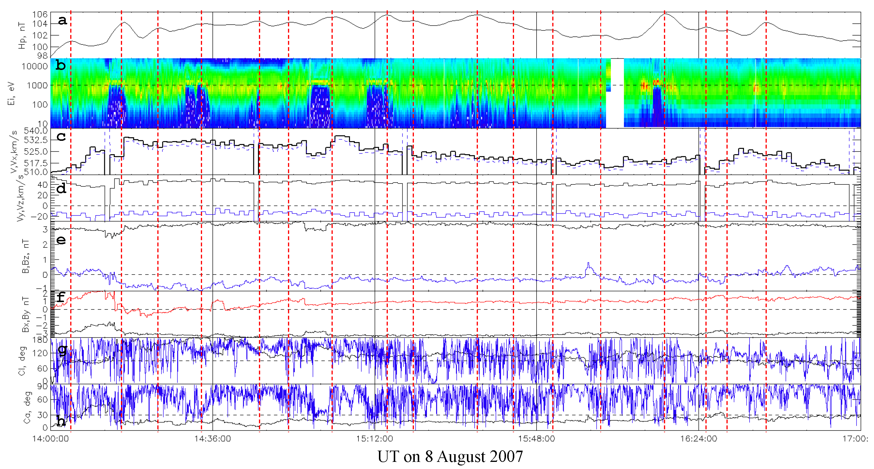
Figure 4 demonstrates an ∼3 h interval of quasi-radial IMF detected by ACE on 8 August 2007. During the rIMF interval, as seen in Figure 4h, the IMF cone angle was fairly smaller (and continuously) than 30°. At the same time, the TH-A probe observed intense fluxes of energetic ions (>10 keV) in the subsolar magnetosheath. The presence of energetic ions indicated effective ion acceleration at a quasi-parallel bow shock in the subsolar region. This supports the quasi-radial IMF orientation at the Earth’s orbit [61]. As seen in Figure 4c, the solar wind velocity varied slightly around 520 km/s, allowing the time for direct propagation of solar wind structures from ACE to the Earth of about = 47 min, which is indicative of strong correlations in the long-time variations of the IMF clock angles measured by ACE in the upstream solar wind and TH-A in the magnetosheath.
ACE did not measure any discontinuities in the time range ∼14:30 UT to 17:00 UT, indicating a quasi-stationarity during the rIMF interval. However, GOES-12 (in a geosynchronous orbit) detected prominent amplitude variations up to several nT in the geomagnetic field (top panel of Figure 4). GOES-12 was moving in the pre-noon sector from 09:00 LT at 14:00 UT to noon at 17:00 UT. The magnetic pulses in the geosynchronous magnetic field (Figure 4a) coincided very often with abrupt enhancements of differential fluxes of ∼1 keV ions in the magnetosheath (yellow and red areas in Figure 4b). This made it clear that the ion enhancements were related to plasma jets, which were generated in the turbulent magnetosheath under quasi-radial IMF and quasi-stationary solar wind.
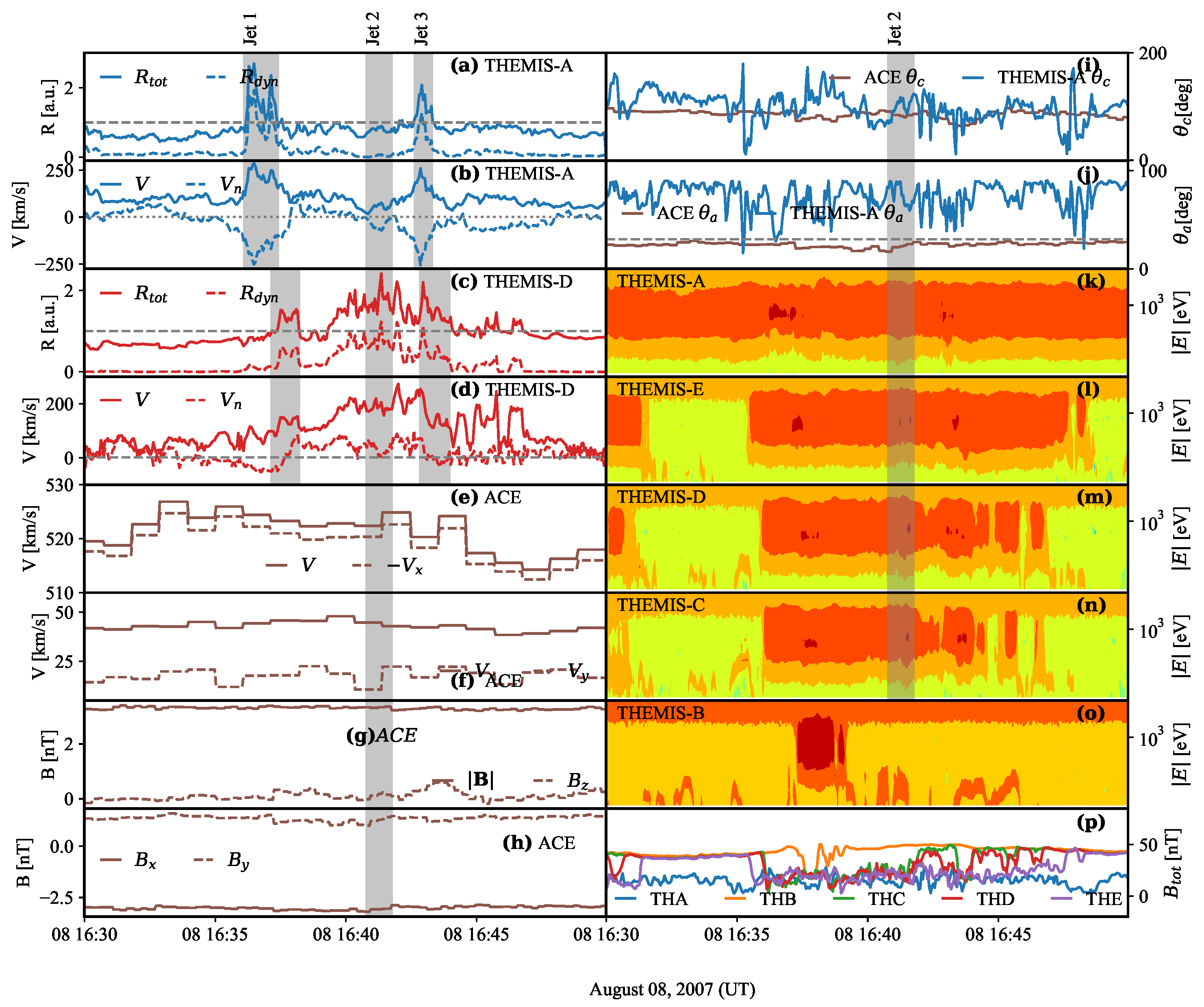
Figure 5 shows a 20 min portion of the long-lasting rIMF interval as an example of a jet generated in the magnetosheath and its interaction with the magnetosphere. On 8 August 2007, from 16:30 UT to 16:50 UT, the chain of THEMIS probes was located near the noon meridian at ∼17° S latitude at , , , and for TH-A, TH-B, TH-C, TH-D and TH-E, respectively. The outermost TH-A probes detected two large-scale plasma jets in the magnetosheath: Jet 1 from 16:36:04 UT to 16:37:26 UT and Jet 3 from 16:42:36 UT to 16:43:20 UT (Figure 5a,b), with total energy ratios of = 2.7 and 2.1, respectively, along with a large component of the plasma velocity normal to the magnetopause, = −250 km/s.
Jets 1 and 3 were observed deeper in the magnetosheath by TH-E, TH-D, and TH-C with a time delay of ∼1 min. The propagation velocity of = −250 km/s presented a time delay that corresponded to a distance of 3 , which was twice the distance of 1.4 between the outermost TH-A and innermost TH-E probes. This suggested that the jets decelerated during the propagation from the magnetosheath to the magnetopause. The deceleration can be found from the measurements of the plasma velocity at the inner THEMIS probes for TH-E, TH-D and TH-C to respectively be −100 km/s, −50 km/s. Note that the innermost TH-B probe located in the magnetosphere at 11.7 observed only the most prominent Jet 1. Before the arrival of Jet 1, the TH-B detected a 10 nT increase of the magnetic field, as shown in Figure 5p.
In the interval from 16:41 UT to 16:42 UT, the probes TH-E, TH-D and TH-C observed Jet 2, which was not seen by the outermost TH-A. It would seem that Jet 2 was formed in the inner regions of the magnetosheath. From the plasma observations of TH-E, TH-D and TH-C, we found that Jet 2 had a small positive . The TH-B probe did not detect any magnetic pulse from 16:41 UT to 16:42 UT. This indicated that Jet 2 did not interact with the magnetopause.
To summarise the case study of quasi-radial IMF generated jets, we identified two large-scale plasma jets, Jet 1 and Jet 3. The interaction of the jets as shown in Figure 4 with the magnetopause produced an integral magnetic pulse at the geosynchronous orbit with an amplitude of ∼4 nT, as was observed by GOES-12 from 16:36 UT to 16:45 UT.
3.4. Collapsing Foreshock
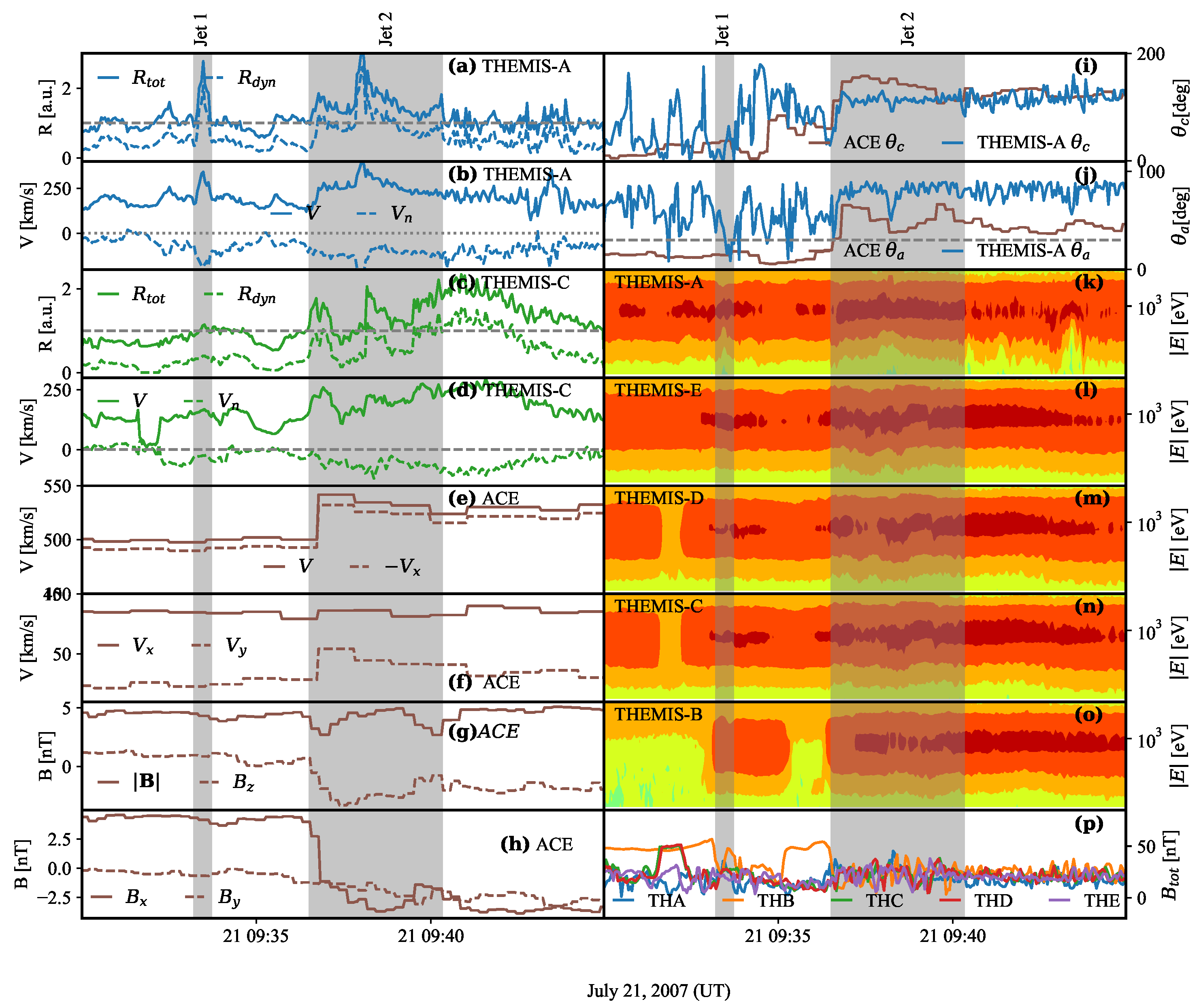
Intervals of quasi-radial IMF can be ended by a directional discontinuity, across which the cone angle increases above 20°, resulting in a collapse of the foreshock in the subsolar region. Figure 6 demonstrates an example of the collapsing FS observed by THEMIS from 09:36 UT to 09:40 UT on 21 July 2007. The chain of THEMIS probes was located slightly southward and duskward from the subsolar point during this time, at a latitude of ∼22° and longitude of ∼13°. The probes TH-A, TH-B, TH-C, TH-D and TH-E had the following coordinates: , , , and , respectively. The innermost TH-B probe was initially located inside the magnetosphere, in disagreement with the model by Lin et al. [36], which predicted the magnetopause location to be away from the THEMIS probes in the order of several . The anomalous expansion of the magnetopause in the present case is an indication of rIMF conditions [17].
Until 09:36 UT, the THEMIS probes detected enhanced fluxes of >10 keV ions inside the magnetosheath (see the plasma spectra in Figure 6) and large amplitude fluctuations of the clock and cone angles of the magnetosheath magnetic field as shown in Figure 6i,j. The strong magnetic fluctuations and enhanced energetic ions in the magnetosheath indicated the presence of the subsolar foreshock, which was generated under the rIMF conditions. The magnetic fluctuations and fluxes of the energetic ions began to diminish at ∼09:36 UT, as observed by the outermost TH-A probe and then consequently by TH-E, TH-D and TH-C at 09:39 UT and by TH-B at 09:40 UT. Apparently, the reduction was related to a change of the IMF orientation from quasi-radial to quasi-perpendicular, which resulted in collapsing of the subsolar foreshock, moving the foreshock region to another place.
As one can see in the top three panels of Figure 6, the outermost TH-A probe detected two jets: Jet 1 from 09:33:12 UT to 09:33:44 UT and Jet 2 from 09:36:48 UT to 09:40:20 UT. Jet 1 was characterised by the energy ratio and a large km/s component. However, Jet 1 faded deeper in the magnetosheath as observed by the other probes (see the plasma spectra in Figure 6) such that km/s at TH-B not shown here for brevity). Thus, Jet 1 did not reach the magnetopause. It would seem that Jet 1 was generated sporadically in the outer magnetosheath under quasi-radial IMF conditions and was then swept away by the magnetosheath plasma streams.
Jet 2 had a very large-scale (duration of ∼3.4 min) and high energy ratio = 2.66, contributed mainly by the kinetic energy km/s, as shown in Figure 6a,b. The jet propagated from the outer magnetosheath towards the Earth with a high speed of km/s and hit the magnetopause. The innermost TH-B probe, located in the magnetosphere, observed Jet 1 from 09:37:15 UT to 09:43:20 UT. At the TH-B location, Jet 1 had decelerated such that km/s and km/s.
We found that Jet 2 was generated during the collapsing FS, which resulted from the discontinuity interaction with the bow shock. We should note here that the identification of discontinuity in the upstream solar wind is difficult because of high uncertainties in the determination of the propagation time under rIMF conditions [53,62]. In order to analyse the nature of discontinuity, we used intervals before and after the discontinuity, respectively, from 08:36 UT to 08:37 UT and from 08:41 UT to 08:42 UT. Before TD, the average IMF vector was nT and after, nT. The normal to the IMF rotation plane . The magnetic field strength changed across the discontinuity from 4.03 nT to 4.68 nT such that . These features indicated that this was a tangential discontinuity. For the given orientation of the TD, the propagation time to the subsolar bow shock was found to be min, in good agreement with the time lag obtained from the cross-correlation. To summarise, we observed the geoeffective Jet 2 generated through the interaction of a TD with the magnetosphere, accompanied with a subsolar foreshock collapse.
3.5. Statistical Analysis
During the THEMIS operations from 2007 to 2009, a total of 554 large-scale geoeffective magnetosheath plasma jets were identified, implying that they interacted with the magnetopause. The jets were further categorised into four categories: tangential discontinuity-mediated 131 jets, 139 related to rotational discontinuities, 110 jets caused by the collapsing foreshock and 174 jets generated under quasi-radial IMF conditions. We found one large-scale jet of unknown origin, possibly related to solar wind conditions, unobserved by upstream monitors, or the propagation time was very unusual, such that the time delay could not be determined. We did not consider this jet of unknown origin in this analysis.
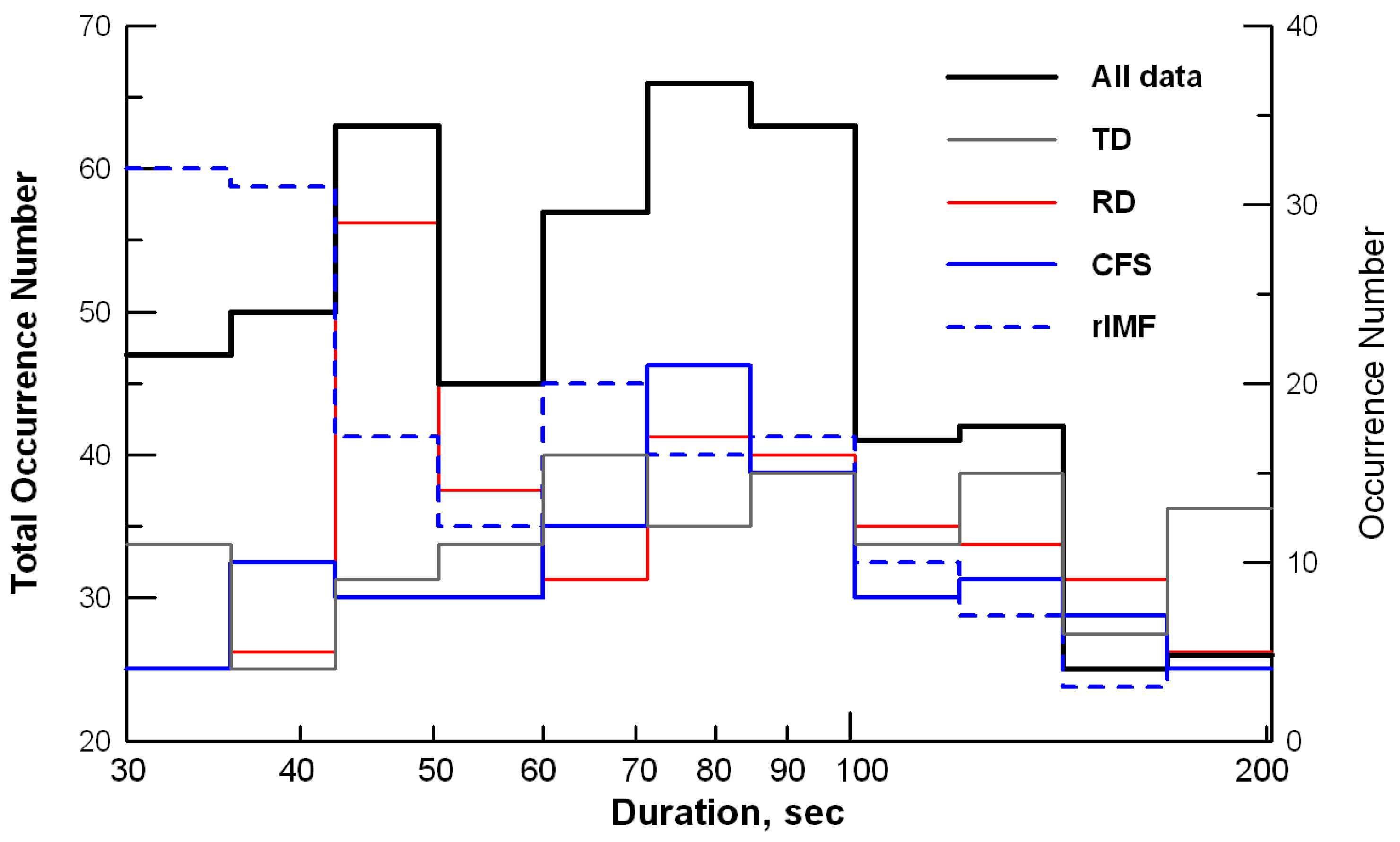
Table 1 shows the statistical distribution of jets originating from different interplanetary structures. We observed that 51% of the jets were mediated by quasi-radial IMF. RDs and TDs produced similar amounts of magnetosheath jets (24% and 25%, respectively). On the other hand, if we considered the CFS structures to be related to discontinuities, then 69% of the jets could be attributed to interplanetary discontinuities and only 31% to rIMF intervals. Thus, at least two-thirds of the large-scale plasma jets were generated in the magnetosheath due to the interaction of interplanetary discontinuities with the magnetosphere. Figure 7 shows a distribution of the jet duration in logarithmic scale. The duration varied from 30 s to more than 3 min and peaked at around 80 s. A secondary maximum can be found around 45 s. The duration of jets generated under rIMF conditions peaked at ∼30 s, which was in good agreement with previous studies [2]. In contrast, the duration of jets related to tangential discontinuities and CFS had a wide maximum between 60 and 100 s. The distribution of the RD-related jets had two maxima: the highest one around 45 s and the second one around 80 s. This implied that the wide maximum duration from 60–100 s was contributed to mainly by jets related to directional discontinuities: TD, RD and CFS. Thus, we suggested that 80 s is a characteristic time of energy conversion during the interaction of interplanetary discontinuities with the magnetosphere. Taking the velocity of the jets to be ∼200–500 km/s, we could estimate the spatial scale of the jets to be ∼3–6∼.
Depending on the origin of the jets, we note that the spatial scales of the jets were different. The jets related to discontinuities were global with respect to magnetospheric scales, whereas most of the rIMF-related jets were local, in accordance with the scale sizes of foreshock structures and bow shock undulations. Thus, the occurrence of rIMF jets might be underestimated, when jets are counted based on in situ observations by a few satellites. Additionally, the localisation of rIMF jets made it harder to determine from in situ observations whether they reached the magnetopause and were geoeffective, because of their more localised impact. Unfortunately, this problem cannot be solved using existing experimental techniques. On the other hand, the geoeffectiveness of small jets on the scale of is debatable, since we have to question how they can pierce more than across the magnetosheath and even if they push against the magnetopause, how prominent their impact is. Thus, the present statistics can be considered as a first approach in the comparison of the geoeffectiveness of jets of different origins.
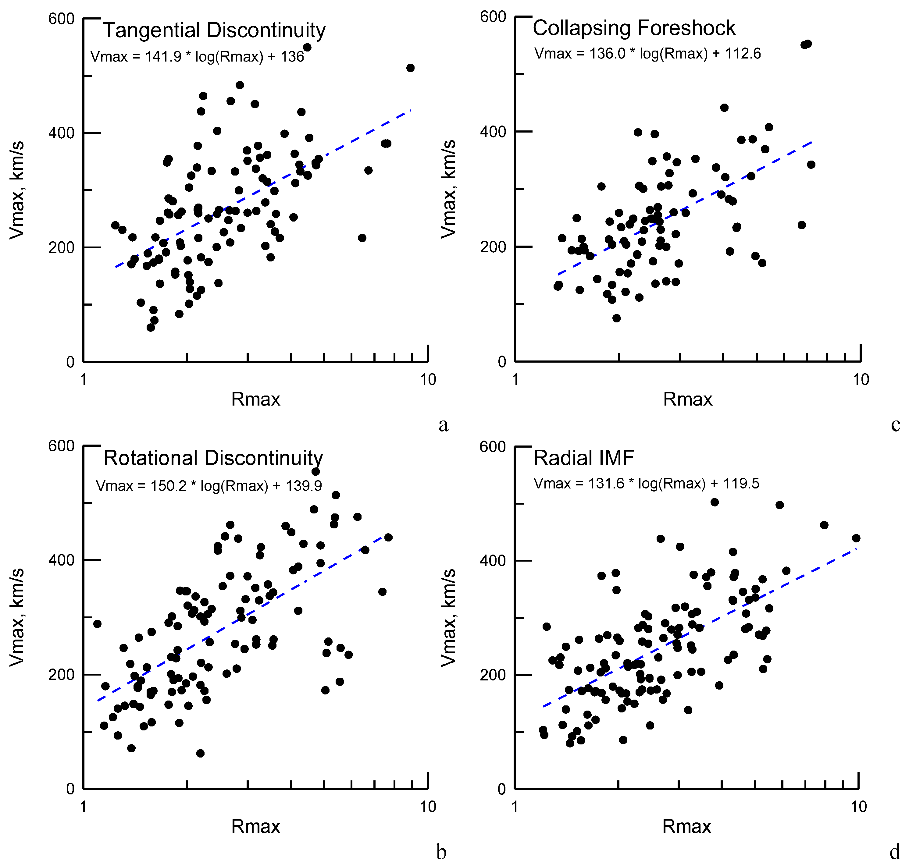
Dmitriev and Suvorova [18] revealed parameters characterising the capability of jet penetration through the magnetopause: the maximal energy ratio Rmax and the maximal velocity of a jet. Figure 8 shows scatter plots of these parameters for different kinds of interplanetary structures. The vary from one to ten, and the jet velocities vary from a few tens to more than 500 km/s. For a quantitative analysis, we fit the scatter plots of versus using a linear regression:
To elucidate, we calculated the averaged values of , and the slope a from Equation (2). Higher and mean a higher capability of a jet to penetrate through the magnetopause. The steeper slope indicates higher jet velocities under larger , that is the higher geoeffectiveness of the jet. It can be easily observed that for different structures are essentially similar: = 2.3 ± 1.6. The jets related to the RD structures have the highest = 275 km/s, and the scatter plot is characterised by the steepest slope of . The lowest = 246 km/s with a slope of can be found for jets generated during rIMF intervals. The CFS-related jets are characteristically similar to those for the rIMF. This similarity is unsurprising, since in both cases, the energy source for jet generation is the same foreshock in the subsolar region. For the TD structures, the and the slope are intermediate. Note that the errors in determination of the slope and especially are large. More statistics are required to increase the accuracy. Hence, the differences presented here are qualitative rather than quantitative and might indicate some bias.
The last column of Table 2 demonstrates the percentage of most powerful jets with . It can be clearly seen that the number of strong jets is two times more often related to RD structures (13%) than the TD and rIMF structures (6% and 7%, respectively). The CFS produced 9% of the powerful jets, but their average velocity km/s was relatively low. Thus, we can conclude that most geoeffective jets are generated in the magnetosheath during the interaction of rotational discontinuities with the magnetosphere. The weakest jets are generated under quasi-radial IMF conditions.
4. Discussion
From the statistical analysis of large-scale plasma jets, we found that the duration of jets varied from 30 s to 3 min and peaked at 80 s. That is different from the statistics of jets collected in the subsolar region, which have a peak duration of 30 s and occur predominantly under quasi-radial IMF [24,28]. The large-scale jets occupy a wide longitudinal range of ∼70° around the subsolar point [18]. The present statistical analysis found that more than two-thirds of the jets were generated in the interaction of interplanetary discontinuities with the bow shock and foreshock. Moreover, the statistical distribution of the duration of rIMF-related jets peaked around 30 s. Thus, it is reasonable to suggest that the origin of large-scale plasma jet is possibly different from the origin of small-scale jets.
Considering the case events of quasi-radial IMF and collapsing foreshock, we found “embedded” jets of an approximate duration of 40 s, which were swept away by the background magnetosheath streams and, thus, did not interact with the magnetopause and, hence, were not geoeffective. As a result, despite the high occurrence rate of jets, quasi-radial IMF intervals produce only ∼30% of geoeffective jets. Moreover, the power of rIMF-related jets had the tendency to be the lowest: the average velocity and the number of jets with was smaller than that for jets related to interplanetary discontinuities.
The deficiency of energy in the rIMF jets might be explained by a kinetic effect of diffuse energetic ions in the foreshock region [41]; that is, the ions are effectively accelerated at the quasi-parallel bow shock up to energies of several keV or higher. These ions move away to the upstream solar wind, as well as go downstream through the magnetopause without interaction. As a result, the energetic ions take a significant portion of the solar wind energy out from the foreshock and the magnetosheath.
The most powerful geoeffective jets tend to be related to rotational discontinuities. In previous studies, a large-scale jet of ∼5 min in duration was found to have been generated via the interaction with an interplanetary rotational discontinuity, which changed the bow shock regime from quasi-parallel (corresponding to quasi-radial IMF) to quasi-perpendicular [12]. As shown by Lin et al. [10], such jets are enforced and extended by a collapsing foreshock. Moreover, the rotational discontinuity-related jets are characterised by a large spatial extension of more than and can produce travelling magnetopause distortions occupying more than half of the dayside hemisphere. Recently, Reference [55] reported the effects of travelling foreshocks and transient foreshock phenomena produced by the interaction of IMF directional discontinuities with the foreshock and bow shock. These observations support the generation mechanism for powerful jets of very large spatial scales well.
5. Conclusions
In conclusion, we analysed four mechanisms of geoeffective magnetosheath jet origins and their evolution through the magnetosphere. Additionally, we presented a statistical study of of such large-scale jets in the period between 2007 and 2009 and determined their mechanisms. We showed that a major portion (69%) of these jets were produced by directional discontinuities and that the quasi-radial IMF and collapsing foreshocks had similar characteristics. This study, while preliminary, can be used to study stellar jets and the roles of plasma discontinuities in producing these jets. We also found that the fastest and strongest jets that impact the Earth’s magnetopause arise from the rotational discontinuities.
Author Contributions
A.V.D. conceptualised and designed the project and performed the initial analysis, and the manuscript was written by A.V.D., B.L. and S.G. All authors have read and agreed to the published version of the manuscript.
Funding
This work was supported by Grant MOST-104-2111-M-008-015- and partially by MOST 109-2111-M-008-005- from the Ministry of Science and Technology of Taiwan and by Ministry of Education under the Aim for Top University program at National Central University of Taiwan.
Informed Consent Statement
No applicable.
Data Availability Statement
The data used in this article are available from CDAWeb, (https://cdaweb.gsfc.nasa.gov/), accessed on 10 February 2019.
Acknowledgments
The authors are grateful to the CDAWeb team (https://cdaweb.gsfc.nasa.gov/, accessed on 15 May 2021) for providing free public data on the magnetic field and plasma measured by the THEMIS mission. We acknowledge NASA Contract NAS5-02099 and V. Angelopoulos for the use of plasma data from the THEMIS mission. We thank K.H. Glassmeier and U. Auster for the use of magnetic FGM data provided under Contract 50 OC 0302 and C. W. Carlson and J. P. McFadden for use of the ESA data. We thank N. Ness and D. J. McComas for the use of ACE solar wind data made available via CDAWeb. The authors are grateful to Howard J. Singer for the opportunity to use the magnetic data from the GOES geosynchronous satellites presented at CDAWeb. The authors are also grateful for Alla Suvorova for many helpful suggestions.
Conflicts of Interest
The authors declare no conflict of interest. The funders had no role in the design of the study; in the collection, analyses, or interpretation of data; in the writing of the manuscript; nor in the decision to publish the results.
References
- Borovsky, J.E.; Valdivia, J.A. The Earth’s Magnetosphere: A Systems Science Overview and Assessment. Surv. Geophys. 2018, 39, 817–859. [Google Scholar] [CrossRef] [Green Version]
- Plaschke, F.; Hietala, H.; Archer, M.; Blanco-Cano, X.; Kajdič, P.; Karlsson, T.; Lee, S.H.; Omidi, N.; Palmroth, M.; Roytershteyn, V.; et al. Jets Downstream of Collisionless Shocks. Space Sci. Rev. 2018, 214, 81. [Google Scholar] [CrossRef] [Green Version]
- Escoubet, C.P.; Hwang, K.J.; Toledo-Redondo, S.; Turc, L.; Haaland, S.E.; Aunai, N.; Dargent, J.; Eastwood, J.P.; Fear, R.C.; Fu, H.; et al. Cluster and MMS Simultaneous Observations of Magnetosheath High Speed Jets and Their Impact on the Magnetopause. Front. Astron. Sp. Sci. 2020, 6, 78. [Google Scholar] [CrossRef] [Green Version]
- Pulkkinen, A.; Lindahl, S.; Viljanen, A.; Pirjola, R. Geomagnetic storm of 29–31 October 2003: Geomagnetically induced currents and their relation to problems in the Swedish high-voltage power transmission system. Sp. Weather 2005, 3. [Google Scholar] [CrossRef]
- Horne, R.B.; Phillips, M.W.; Glauert, S.A.; Meredith, N.P.; Hands, A.D.P.; Ryden, K.A.; Li, W. Realistic Worst Case for a Severe Space Weather Event Driven by a Fast Solar Wind Stream. Sp. Weather 2018, 16, 1202–1215. [Google Scholar] [CrossRef] [PubMed] [Green Version]
- Tsurutani, B.; Lakhina, G.; Verkhoglyadova, O.; Gonzalez, W.; Echer, E.; Guarnieri, F. A review of interplanetary discontinuities and their geomagnetic effects. J. Atmos. Solar-Terrestrial Phys. 2011, 73, 5–19. [Google Scholar] [CrossRef]
- Archer, M.O.; Horbury, T.S.; Eastwood, J.P. Magnetosheath pressure pulses: Generation downstream of the bow shock from solar wind discontinuities. J. Geophys. Res. Sp. Phys. 2012, 117, 1–13. [Google Scholar] [CrossRef]
- Sibeck, D.G.; Kudela, K.; Lepping, R.P.; Lin, R.; Nemecek, Z.; Nozdrachev, M.N.; Phan, T.D.; Prech, L.; Safrankova, J.; Singer, H.; et al. Magnetopause motion driven by interplanetary magnetic field variations. J. Geophys. Res. Sp. Phys. 2000, 105, 25155–25169. [Google Scholar] [CrossRef]
- Savin, S.; Amata, E.; Zelenyi, L.; Lutsenko, V.; Safrankova, J.; Nemecek, Z.; Borodkova, N.; Buechner, J.; Daly, P.W.; Kronberg, E.A.; et al. Super fast plasma streams as drivers of transient and anomalous magnetospheric dynamics. Ann. Geophys. 2012, 30, 1–7. [Google Scholar] [CrossRef]
- Lin, Y.; Swift, D.W.; Lee, L.C. Simulation of pressure pulses in the bow shock and magnetosheath driven by variations in interplanetary magnetic field direction. J. Geophys. Res. Sp. Phys. 1996, 101, 27251–27269. [Google Scholar] [CrossRef]
- Tsubouchi, K.; Matsumoto, H. Effect of upstream rotational field on the formation of magnetic depressions in a quasi- Perpendicular shock downstream. J. Geophys. Res. Sp. Phys. 2005, 110, 1–11. [Google Scholar] [CrossRef] [Green Version]
- Dmitriev, A.V.; Suvorova, A.V. Traveling magnetopause distortion related to a large-scale magnetosheath plasma jet: THEMIS and ground-based observations. J. Geophys. Res. Sp. Phys. 2012, 117, 1–16. [Google Scholar] [CrossRef] [Green Version]
- Neugebauer, M.; Clay, D.R.; Tsurutani, B.T.; Zwickl, R.D.; Goldstein, B.E. Reexamination of Rotational and Tangential Discontinuities in the Solar Wind. J. Geophys. Res. 1984, 89, 5395–5408. [Google Scholar] [CrossRef]
- Artemyev, A.V.; Angelopoulos, V.; Vasko, I.Y. Kinetic Properties of Solar Wind Discontinuities at 1 AU Observed by ARTEMIS. J. Geophys. Res. Sp. Phys. 2019, 124, 3858–3870. [Google Scholar] [CrossRef]
- Neukirch, T.; Vasko, I.Y.; Artemyev, A.V.; Allanson, O. Kinetic models of tangential discontinuities in the solar wind. Astrophys. J. 2020, 891, 86. [Google Scholar] [CrossRef]
- Neugebauer, M. The structure of rotational discontinuities. Geophys. Res. Lett. 1989, 16, 1261–1264. [Google Scholar] [CrossRef]
- Suvorova, A.V.; Shue, J.H.; Dmitriev, A.V.; Sibeck, D.G.; McFadden, J.P.; Hasegawa, H.; Ackerson, K.; Jelínek, K.; Šafráková, J.; Němeček, Z. Magnetopause expansions for quasi-radial interplanetary magnetic field: THEMIS and Geotail observations. J. Geophys. Res. Sp. Phys. 2010, 115, 1–16. [Google Scholar] [CrossRef] [Green Version]
- Dmitriev, A.V.; Suvorova, A.V. Large-scale jets in the magnetosheath and plasma penetration across the magnetopause: THEMIS observations. J. Geophys. Res. Sp. Phys. 2015, 120, 4423–4437. [Google Scholar] [CrossRef] [Green Version]
- Eastwood, J.P.; Nakamura, R.; Turc, L.; Mejnertsen, L.; Hesse, M. The Scientific Foundations of Forecasting Magnetospheric Space Weather. Space Sci. Rev. 2017, 212, 1221–1252. [Google Scholar] [CrossRef] [Green Version]
- Sibeck, D.G.; Trivedi, N.B.; Zesta, E.; Decker, R.B.; Singer, H.J.; Szabo, A.; Tachihara, H.; Watermann, J. Pressure-pulse interaction with the magnetosphere and ionosphere. J. Geophys. Res. Sp. Phys. 2003, 108, 1–12. [Google Scholar] [CrossRef] [Green Version]
- Eastwood, J.P.; Sibeck, D.G.; Angelopoulos, V.; Phan, T.D.; Bale, S.D.; McFadden, J.P.; Cully, C.M.; Mende, S.B.; Larson, D.; Frey, S.; et al. THEMIS observations of a hot flow anomaly: Solar wind, magnetosheath, and ground-based measurements. Geophys. Res. Lett. 2008, 35, 1–5. [Google Scholar] [CrossRef] [Green Version]
- Jacobsen, K.S.; Phan, T.D.; Eastwood, J.P.; Sibeck, D.G.; Moen, J.I.; Angelopoulos, V.; McFadden, J.P.; Engebretson, M.J.; Provan, G.; Larson, D.; et al. THEMIS observations of extreme magnetopause motion caused by a hot flow anomaly. J. Geophys. Res. Sp. Phys. 2009, 114. [Google Scholar] [CrossRef]
- Archer, M.O.; Horbury, T.S.; Eastwood, J.P.; Weygand, J.M.; Yeoman, T.K. Magnetospheric response to magnetosheath pressure pulses: A low-pass filter effect. J. Geophys. Res. Sp. Phys. 2013, 118, 5454–5466. [Google Scholar] [CrossRef] [Green Version]
- Plaschke, F.; Hietala, H.; Angelopoulos, V. Anti-sunward high-speed jets in the subsolar magnetosheath. Ann. Geophys. 2013, 31, 1877–1889. [Google Scholar] [CrossRef] [Green Version]
- Savin, S.; Amata, E.; Zelenyi, L.; Budaev, V.; Consolini, G.; Treumann, R.; Lucek, E.; Safrankova, J.; Nemecek, Z.; Khotyaintsev, Y.; et al. High energy jets in the Earth’s magnetosheath: Implications for plasma dynamics and anomalous transport. JETP Lett. 2008, 87, 593–599. [Google Scholar] [CrossRef] [Green Version]
- Hietala, H.; Plaschke, F. On the generation of magnetosheath high-speed jets by bow shock ripples. J. Geophys. Res. Sp. Phys. 2013, 118, 7237–7245. [Google Scholar] [CrossRef] [Green Version]
- Lucek, E.A.; Horbury, T.S.; Dandouras, I.; Réme, H. Cluster observations of the Earth’s quasi-parallel bow shock. J. Geophys. Res. Sp. Phys. 2008, 113, 1–11. [Google Scholar] [CrossRef] [Green Version]
- Archer, M.O.; Horbury, T.S. Magnetosheath dynamic pressure enhancements: Occurrence and typical properties. Ann. Geophys. 2013, 31, 319–331. [Google Scholar] [CrossRef]
- Pi, G.; Shue, J.H.; Chao, J.K.; Němeček, Z.; Šafránková, J.; Lin, C.H. A reexamination of long-duration radial IMF events. J. Geophys. Res. Sp. Phys. 2014, 119, 7005–7011. [Google Scholar] [CrossRef]
- Angelopoulos, V. The THEMIS Mission. Space Sci. Rev. 2008, 141, 5–34. [Google Scholar] [CrossRef]
- Stone, E.C.; Frandsen, A.M.; Mewaldt, R.A.; Christian, E.R.; Margolies, D.; Ormes, J.F.; Snow, F. The Advanced Composition Explorer. Space Sci. Rev. 1998, 86, 1–22. [Google Scholar] [CrossRef]
- Lepping, R.P.; Acũna, M.H.; Burlaga, L.F.; Farrell, W.M.; Slavin, J.A.; Schatten, K.H.; Mariani, F.; Ness, N.F.; Neubauer, F.M.; Whang, Y.C.; et al. The WIND magnetic field investigation. Space Sci. Rev. 1995, 71, 207–229. [Google Scholar] [CrossRef]
- Auster, H.U.; Glassmeier, K.H.; Magnes, W.; Aydogar, O.; Baumjohann, W.; Constantinescu, D.; Fischer, D.; Fornacon, K.H.; Georgescu, E.; Harvey, P.; et al. The THEMIS fluxgate magnetometer. Space Sci. Rev. 2008, 141, 235–264. [Google Scholar] [CrossRef]
- McFadden, J.P.; Carlson, C.W.; Larson, D.; Ludlam, M.; Abiad, R.; Elliott, B.; Turin, P.; Marckwordt, M.; Angelopoulos, V. The THEMIS ESA plasma instrument and in-flight calibration. Space Sci. Rev. 2008, 141, 277–302. [Google Scholar] [CrossRef]
- Chao, J.K.; Wu, D.J.; Lin, C.H.; Yang, Y.H.; Wang, X.Y.; Kessel, M.; Chen, S.H.; Lepping, R.P. Models for the size and shape of the earth’s magnetopause and bow shock. COSPAR Colloq. Ser. 2002, 12, 127–135. [Google Scholar] [CrossRef] [Green Version]
- Lin, R.L.; Zhang, X.X.; Liu, S.Q.; Wang, Y.L.; Gong, J.C. A three-dimensional asymmetric magnetopause model. J. Geophys. Res. Sp. Phys. 2010, 115. [Google Scholar] [CrossRef]
- Dmitriev, A.V.; Chao, J.K.; Wu, D.J. Comparative study of bow shock models using Wind and Geotail observations. J. Geophys. Res. Sp. Phys. 2003, 108, 1–19. [Google Scholar] [CrossRef]
- Escoubet, C.P.; Schmidt, R.; Goldstein, M.L. Cluster—Science and Mission Overview. In The Cluster and Phoenix Missions; Springer: Dordrecht, The Netherlands, 1997; Volume 79, pp. 11–32. [Google Scholar] [CrossRef]
- Burch, J.L.; Moore, T.E.; Torbert, R.B.; Giles, B.L. Magnetospheric Multiscale Overview and Science Objectives. Space Sci. Rev. 2016, 199, 5–21. [Google Scholar] [CrossRef] [Green Version]
- Lu, S.W.; Wang, C.; Li, W.Y.; Tang, B.B.; Torbert, R.B.; Giles, B.L.; Russell, C.T.; Burch, J.L.; McFadden, J.P.; Auster, H.U.; et al. Prolonged Kelvin–Helmholtz Waves at Dawn and Dusk Flank Magnetopause: Simultaneous Observations by MMS and THEMIS. Astrophys. J. 2019, 875, 57. [Google Scholar] [CrossRef]
- Dmitriev, A.V.; Lin, R.L.; Liu, S.Q.; Suvorova, A.V. Model prediction of geosynchronous magnetopause crossings. Sp. Weather 2016, 14, 530–543. [Google Scholar] [CrossRef] [Green Version]
- Plaschke, F.; Hietala, H.; Angelopoulos, V.; Nakamura, R. Geoeffective jets impacting the magnetopause are very common. J. Geophys. Res. Sp. Phys. 2016, 121, 3240–3253. [Google Scholar] [CrossRef]
- Burton, R.K.; McPherron, R.L.; Russell, C.T. An empirical relationship between interplanetary conditions and Dst. J. Geophys. Res. 1975, 80, 4204–4214. [Google Scholar] [CrossRef]
- Shue, J.H.; Chao, J.K.; Song, P.; McFadden, J.P.; Suvorova, A.; Angelopoulos, V.; Glassmeier, K.H.; Plaschke, F. Anomalous magnetosheath flows and distorted subsolar magnetopause for radial interplanetary magnetic fields. Geophys. Res. Lett. 2009, 36, 3–7. [Google Scholar] [CrossRef] [Green Version]
- Voitcu, G.; Echim, M. Tangential deflection and formation of counterstreaming flows at the impact of a plasma jet on a tangential discontinuity. Geophys. Res. Lett. 2017, 44, 5920–5927. [Google Scholar] [CrossRef] [Green Version]
- Yang, L.; Zhang, L.; He, J.; Tu, C.; Wang, L.; Marsch, E.; Wang, X.; Zhang, S.; Feng, X. The formation of rotational discontinuities in compressive three-dimensional mhd turbulence. Astrophys. J. 2015, 809, 155. [Google Scholar] [CrossRef] [Green Version]
- Plaschke, F.; Karlsson, T.; Hietala, H.; Archer, M.; Vörös, Z.; Nakamura, R.; Magnes, W.; Baumjohann, W.; Torbert, R.B.; Russell, C.T.; et al. Magnetosheath High-Speed Jets: Internal Structure and Interaction with Ambient Plasma. J. Geophys. Res. Sp. Phys. 2017, 122, 10,157–10,175. [Google Scholar] [CrossRef]
- Vuorinen, L.; Hietala, H.; Plaschke, F. Jets in the magnetosheath: IMF control of where they occur. Ann. Geophys. 2019, 37, 689–697. [Google Scholar] [CrossRef] [Green Version]
- Walén, C. On the Theory of Sunspots. Arkiv för Matematik Astronomi och Fysik 1944, 30A, 1–87. [Google Scholar]
- Crooker, N.U.; Eastman, T.E.; Frank, L.A.; Smith, E.J.; Russell, C.T. Energetic magnetosheath ions and the interplanetary magnetic field orientation. J. Geophys. Res. Sp. Phys. 1981, 86, 4455–4460. [Google Scholar] [CrossRef]
- Terasawa, T. Energy spectrum of ions accelerated through Fermi process at the terrestrial bow shock. J. Geophys. Res. Sp. Phys. 1981, 86, 7595–7606. [Google Scholar] [CrossRef]
- Fuselier, S.A.; Lennartsson, O.W.; Thomsen, M.F.; Russell, C.T. He2+ heating at a quasi-parallel shock. J. Geophys. Res. 1991, 96, 9805. [Google Scholar] [CrossRef]
- Suvorova, A.V.; Dmitriev, A.V. On magnetopause inflation under radial IMF. Adv. Sp. Res. 2016, 58, 249–256. [Google Scholar] [CrossRef]
- Jelínek, K.; Němeček, Z.; Šafránková, J.; Shue, J.H.; Suvorova, A.V.; Sibeck, D.G. Thin magnetosheath as a consequence of the magnetopause deformation: THEMIS observations. J. Geophys. Res. Sp. Phys. 2010, 115. [Google Scholar] [CrossRef]
- Kajdič, P.; Blanco-Cano, X.; Omidi, N.; Rojas-Castillo, D.; Sibeck, D.G.; Billingham, L. Traveling Foreshocks and Transient Foreshock Phenomena. J. Geophys. Res. Sp. Phys. 2017, 122, 9148–9168. [Google Scholar] [CrossRef] [Green Version]
- Sonnerup, B.; Scheible, M. Minimum and maximum variance analysis. Anal. Methods Multi-Spacecr. Data 1998, 1, 185–220. [Google Scholar]
- Weimer, D.R.; Ober, D.M.; Maynard, N.C.; Burke, W.J.; Collier, M.R.; McComas, D.J.; Ness, N.F.; Smith, C.W. Variable time delays in the propagation of the interplanetary magnetic field. J. Geophys. Res. Sp. Phys. 2002, 107. [Google Scholar] [CrossRef]
- Knetter, T.; Neubauer, F.M.; Horbury, T.; Balogh, A. Four-point discontinuity observations using Cluster magnetic field data: A statistical survey. J. Geophys. Res. Sp. Phys. 2004, 109, 1–12. [Google Scholar] [CrossRef]
- Sergeev, V.A.; Sormakov, D.A.; Apatenkov, S.V.; Baumjohann, W.; Nakamura, R.; Runov, A.V.; Mukai, T.; Nagai, T. Survey of large-amplitude flapping motions in the midtail current sheet. Ann. Geophys. 2006, 24, 2015–2024. [Google Scholar] [CrossRef] [Green Version]
- Sonnerup, B.U.Ö. Orientation and motion of two-dimensional structures in a space plasma. J. Geophys. Res. 2005, 110, A06208. [Google Scholar] [CrossRef] [Green Version]
- Gosling, J.T.; Asbridge, J.R.; Bame, S.J.; Paschmann, G.; Sckopke, N. Observations of two distinct populations of bow shock ions in the upstream solar wind. Geophys. Res. Lett. 1978, 5, 957–960. [Google Scholar] [CrossRef]
- Riazantseva, M.O.; Dalin, P.A.; Dmitriev, A.V.; Orlov, Y.V.; Paularena, K.I.; Richardson, J.D.; Zastenker, G.N. A multifactor analysis of parameters controlling solar wind ion flux correlations using an artificial neural network technique. J. Atmos. Sol.-Terr. Phys. 2002, 64, 657–660. [Google Scholar] [CrossRef]
Figure 1.
Position of the THEMIS probes according the magnetopause model of Lin et al. [36] (in black) in aberrated-GSM coordinates [37] in units of Earth radii () for the four demonstrative cases. We consistently use the following colour scheme for the rest of the figures: TH-A (blue), TH-B (orange), TH-C (green), TH-D (red), and TH-E (purple).

Figure 2.
ACE (in the upstream solar wind) and THEMIS (in the magnetosheath and magnetosphere) observations of plasma and magnetic fields for 23 June 2007 (see the text for the details of the definitions and explanations). The panels (a), and (c) represent , and for TH-B, and TH-C respectively; panels (b) and (d) represent , and for TH-B and TH-C respectively; (e) (ACE is represented by brown curves in the panels (e–j)). , and its component are represented in (e). The panel (f) shows and in the solar wind; (g) represents and ; (h) the interplanetary magnetic fields and ; (i) the clock angle , and (j) cone angle measured by ACE (brown) and the outermost THEMIS probe (TH-B in this case in orange) respectively. The panels (k–o) show the ion spectra measured in the magnetosphere and magnetosheath by TH-B, TH-D, TH-C, TH-E and TH-A respectively. Panel (p) shows as measured by the five THEMIS probes (using the colour schemes mentioned in the caption of Figure 1). Vertical grey bars indicate two large-scale magnetosheath plasma jets: Jet 1 and Jet 2. Vertical rose bar indicates a tangential discontinuity as can be seen from 06:23 UT to 06:25 UT.

Figure 3.
The panels (a–p) represent the same quantities as in Figure 2, but for 5 July 2007 and the panels (a–d) represent the quantities for TH-B and TH-E. The colour scheme is the same as mentioned in Figure 1. The magnetosheath measurements are shown for the above mentioned THEMIS probes, with a time delay for the ACE data of 42 min. Vertical grey dashed lines indicate directional discontinuities (DD1 to DD5) in the upstream solar wind. The discontinuities produce jets in the magnetosheath (Jet 1 to Jet 5), which are observed by the TH-B probe. Vertical grey bars indicate Jet 4 observed by different probes. Vertical green and blue bars indicate the ranges for the analysis of a rotational discontinuity (see the details in the text).

Figure 4.
Plasma and magnetic field on 8 August 2007 as observed by ACE, TH-A and GOES-12 in the upstream solar wind, magnetosheath and at the geosynchronous orbits, respectively. The panels show: (a) horizontal component of GOES-12 geomagnetic field; (b) ion spectrum measured by TH-A; (c) SW bulk velocity and (black and blue curves, respectively); (d) solar wind and (black and blue curves, respectively); (e) IMF and (black and blue curves, respectively); (f) and (black and red curves, respectively); (g) measured by ACE and TH-A (black and blue curves, respectively); (h) measured by ACE and TH-A (black and blue curves, respectively). The time delay for the ACE data is 47 min. The IMF was quasi-radial ( < 30°) most of time, which resulted in intense fluxes of energetic ions (>10 keV) as observed by TH-A. Vertical red dashed lines indicate pulses in horizontal component of the GOES-12 geomagnetic field. Most of the pulses coincide with abrupt enhancements of ∼1 keV ions in the magnetosheath related to plasma jets.

Figure 5.
Panels (a–p) represent the same quantities as in Figure 2, but for 8 August 2007, and for magnetosheath measurements done by the THEMIS probes are represented with TH-A and TH-D with the colour scheme mentioned in Figure 1.

Figure 6.
The panels (a–p) represent the same quantities as in Figure 2, but for 21 July 2007. The magnetosheath measurements are shown for the TH-A and TH-C probes. The time delay for the ACE data is 57.5 min. but for 21 July 2007.
Figure 6.
The panels (a–p) represent the same quantities as in Figure 2, but for 21 July 2007. The magnetosheath measurements are shown for the TH-A and TH-C probes. The time delay for the ACE data is 57.5 min. but for 21 July 2007.

Figure 7.
Statistical distribution of the duration of large-scale plasma jets in the magnetosheath: all jets (black histogram, left axis), jets related to tangential discontinuities (grey histogram, right axis), jets related to rotational discontinuities (red histogram, right axis), jets related to collapsing foreshock (blue histogram, right axis) and jets generated under radial IMF (dashed blue histogram, right axis).

Figure 8.
Scatter plots of maximal velocities Vmax of jets versus maximal energy ratio Rmax for different kinds of jets: (a) related to tangential discontinuities, (b) related to rotational discontinuities, (c) related to collapsing foreshock and (d) generated under radial IMF.
Figure 8.
Scatter plots of maximal velocities Vmax of jets versus maximal energy ratio Rmax for different kinds of jets: (a) related to tangential discontinuities, (b) related to rotational discontinuities, (c) related to collapsing foreshock and (d) generated under radial IMF.


Table 1.
Statistics of jets related to different interplanetary structures.
| Structure | Type | Number | Percentage (Structure) | Percentage |
|---|---|---|---|---|
| Discontinuities | RD | 131 | 24% | 49% |
| TD | 139 | 25% | ||
| Quasi-radial IMF | CFS | 110 | 20% | 51% |
| rIMF | 174 | 31% |
Table 2.
Characteristic number of jets of various origins.
| Structure | Slope | Vmax | Rmax | Rmax > 5 |
|---|---|---|---|---|
| RD | 150 ± 17 | 275 ± 110 | 2.3 ± 1.6 | 13% |
| TD | 142 ± 20 | 265 ± 102 | 2.4 ± 1.5 | 6% |
| CFS | 136 ± 20 | 245 ± 92 | 2.4 ± 1.5 | 9% |
| rIMF | 132 ± 15 | 246 ± 91 | 2.3 ± 1.6 | 7% |
Publisher’s Note: MDPI stays neutral with regard to jurisdictional claims in published maps and institutional affiliations. |
© 2021 by the authors. Licensee MDPI, Basel, Switzerland. This article is an open access article distributed under the terms and conditions of the Creative Commons Attribution (CC BY) license (https://creativecommons.org/licenses/by/4.0/).
Share and Cite
MDPI and ACS Style
Dmitriev, A.V.; Lalchand, B.; Ghosh, S. Mechanisms and Evolution of Geoeffective Large-Scale Plasma Jets in the Magnetosheath. Universe 2021, 7, 152. https://0-doi-org.brum.beds.ac.uk/10.3390/universe7050152
AMA Style
Dmitriev AV, Lalchand B, Ghosh S. Mechanisms and Evolution of Geoeffective Large-Scale Plasma Jets in the Magnetosheath. Universe. 2021; 7(5):152. https://0-doi-org.brum.beds.ac.uk/10.3390/universe7050152
Chicago/Turabian StyleDmitriev, Alexei V., Bhavana Lalchand, and Sayantan Ghosh. 2021. "Mechanisms and Evolution of Geoeffective Large-Scale Plasma Jets in the Magnetosheath" Universe 7, no. 5: 152. https://0-doi-org.brum.beds.ac.uk/10.3390/universe7050152
Note that from the first issue of 2016, this journal uses article numbers instead of page numbers. See further details here.