
Taxonomy of Dark Energy Models
by
 , ,
, ,
Verónica Motta
1,* ,
,
Miguel A. García-Aspeitia
2,3,
Alberto Hernández-Almada
4,
Juan Magaña
5 and
Tomás Verdugo
6 1
Instituto de Física y Astronomía, Facultad de Ciencias, Universidad de Valparaíso, Avda. Gran Bretaña 1111, Valparaíso 2360102, Chile
2
Unidad Académica de Física, Universidad Autónoma de Zacatecas, Calzada Solidaridad Esquina con Paseo a la Bufa S/N, Zacatecas 98060, Mexico
3
Consejo Nacional de Ciencia y Tecnología, Av. Insurgentes Sur 1582. Colonia Crédito Constructor, Del. Benito Juárez, Ciudad de México 03940, Mexico
4
Facultad de Ingeniería, Universidad Autónoma de Querétaro, Centro Universitario Cerro de las Campanas, Santiago de Querétaro 76010, Mexico
5
Instituto de Astrofísica & Centro de Astro-Ingeniería, Pontificia Universidad Católica de Chile, Av. Vicuña Mackenna, Santiago 4860, Chile
6
Instituto de Astronomía, Observatorio Astronómico Nacionál, Universidad Nacional Autónoma de México, Apartado Postal 106, Ensenada 22800, Mexico
*
Author to whom correspondence should be addressed.
Universe 2021, 7(6), 163; https://0-doi-org.brum.beds.ac.uk/10.3390/universe7060163
Submission received: 22 March 2021
/
Revised: 6 April 2021
/
Accepted: 6 April 2021
/
Published: 26 May 2021
(This article belongs to the Special Issue Probing the Dark Universe with Theory and Observations)
Abstract
:The accelerated expansion of the Universe is one of the main discoveries of the past decades, indicating the presence of an unknown component: the dark energy. Evidence of its presence is being gathered by a succession of observational experiments with increasing precision in its measurements. However, the most accepted model for explaining the dynamic of our Universe, the so-called Lambda cold dark matter, faces several problems related to the nature of such energy component. This has led to a growing exploration of alternative models attempting to solve those drawbacks. In this review, we briefly summarize the characteristics of a (non-exhaustive) list of dark energy models as well as some of the most used cosmological samples. Next, we discuss how to constrain each model’s parameters using observational data. Finally, we summarize the status of dark energy modeling.
1. Introduction
One of the most important discoveries in modern cosmology since the observation of the Universe expansion by George Lemaître [1] and Edwin Hubble [2] and the detection of the cosmic microwave background (CMB) [3,4] is the accelerated expansion at late times. This cosmic acceleration was detected at the end of the 1990s, when two independent collaborations were observing high redshift type Ia supernovae (SNIa) to measure the curvature and deceleration parameter of the Universe [5,6]; both groups established a cosmological constant model of the Universe, with 0.3, and 0.7. Later, this result was confirmed by different cosmological probes, for example the CMB [7,8], baryon acoustic oscillations (e.g., [9,10]), and gravitational lensing, both strong (e.g., [11]) and weak (e.g., [12]).
In recent decades, substantial effort has been made to understand the nature of Dark Energy (DE) (e.g., see [13] for a recent review) with the Cold Dark Matter model (CDM) being the cornerstone of modern cosmology and the simplest one, composed of two dominant components, known as cold dark matter (DM) and cosmological constant, and three subdominant components identified as baryons, photons, and neutrinos. The CDM model is not only effective at background level (isotropic and homogeneous Universe), but also robust at linear perturbations, having accurate predictions for the matter power spectrum and the small differences for photons temperature observed in the CMB [14,15]. As mentioned previously, the CDM model is composed of ∼32% cold dark matter, which is essential for the structure formation, being the most suitable explanation for the rotation curves of galaxies (see for instance [16,17,18]). It is assumed that dark matter is a non-relativistic particle and the preferred candidates are the particles emerging from the Supersymmetric theory [19,20]. However, the lack of evidence of these particles strengthens the proposition of other candidates such as Axions, Ultra light scalar field dark matter, and others [21,22,23]. Despite the remarkable achievements of the CDMmodel, it has important afflictions when describing the nature of the cosmological constant (CC) through the idea of a quantum vacuum fluctuations [24,25]. This idea generates, from the theoretical point of view, an error of ∼ orders of magnitude, and it is known as the fine tuning problem [26]. In addition, the CC has the coincidence problem [26], i.e., why did the Universe accelerate at late epochs and not before of after? On top of that, recent observations from Planck and Supernovae Type Ia differ in their values for (see also [27,28] for recent values measured using gravitational lens systems), introducing tension between different observations at different redshifts [29,30,31,32,33]. The community attributes the problem to the CDM model and in particular to the CC; therefore, new approaches are proposed to alleviate the discrepancy among observations (see also [34,35,36]).
In the context of these tensions and the problems with CC, a plethora of alternative dark energy models have been explored. Our aim is to review a set of those models consisting of fluids that can be described by a variety of formulations. Some of them can be described by different fluids and their particles that compose them, like scalar fields, while others that do not need extra fluids but require modifications to general theory of relativity (GTR, [37,38,39,40,41,42,43,44,45,46,47,48,49,50]) (for recent overviews of GTR, see, e.g., [51,52,53] and references therein). Specifically, the first category contains models avoiding the idea of associating the Universe acceleration with quantum vacuum fluctuations (like in CC) and thus assume a fluid expression manageable by the quantum field theory. The second one consist of models introducing extensions to GTR, generating a Universe acceleration without the addition of extra fluids. However, the current overabundance of models is overwhelming, posing difficulties to decide which is the best candidate to compete against the CDM model.
Recent years have also witnessed the increase in observational surveys designed to obtain precise measurements aimed to probe DE’s nature. With this improvement in the instrument sensitivity came the mechanism to discriminate between models of DE; i.e., tensions between different probes could lead to ruling out some of them. In this context, we consider widely used samples (such as SNIa [5], CMB [15], baryon acoustic oscillations) as well as other recent compilations (strong gravitational lens systems [54,55,56], starburst galaxies [57,58,59,60,61,62], and observational Hubble parameters [56,63].
The outline of the review is as follows: Section 2 summarizes the basic equations, Section 3 presents the cosmological samples that we use to constraint the different theoretical models, and Section 4 describes the DE models, together with the constraints of the free parameters of each model. Finally, in Section 5, we give a discussion and conclusion of the models mentioned, discussing the promising models and what the contribution is to the understanding of the Universe acceleration.
2. Basic Equations for the Background Cosmology
Modern cosmology is based on the general theory of relativity, whose master equation is the field equation given by
where is known as the Einstein tensor, composed of the Ricci tensor (), the Ricci scalar (R), and the metric tensor (). The right side of Equation (1) shows the Newton gravitational constant (G) and the energy momentum tensor. Hereafter we will use natural units (), unless we explicitly mention the opposite.
Hereafter, we focus our attention on the background cosmology considering a homogeneous and isotropic Universe. In this vein, we use the standard line element of Friedmann–Lemaitre–Robertson–Walker (FLRW) with flat geometry , as
where and is the scale factor. The energy-momentum tensor is written, as always, as
where p, , , and are the pressure, density, four-velocity of the fluid, and the metric tensor, respectively. The covariant derivative of the energy momentum tensor generates the continuity equation, given by
where the sum is over all the species, and dots stand for derivatives with respect to time.
Through the Einstein field equations, we arrive at the Friedmann equation, which is a first-order non-linear differential equation composed of the scale factor and the densities of the species. Therefore, the equation takes the form
where H is known as the Hubble parameter, which indicates the Universe expansion rate. Hence, it is possible to define the dimensionless Friedmann equation in the form
where is known as the density parameter, a function of the redshift (z), and the sum runs for the components of the Universe used in the model (, , , represent baryons, dark matter, radiation, and dark energy, respectively), is the Hubble constant (this is the Hubble parameter evaluated at ). With the previous equations, it is possible to define the flat condition as
notice that the density parameters are evaluated at and they are denoted with the label 0. The comoving distance from the observer to redshift z is given by (units of c are recovered in the following equations)
Therefore, we define the luminosity distance, denoted as , as
where c is the speed of light. The angular diameter distance is related to the comoving distance as
In addition, the angular diameter distance between two objects at redshifts and () is given by
3. Cosmological Samples
Observational samples are required not only to investigate the consistency of any theoretical model prediction but also to discern between different models. In this section, we review the most common samples used as “standard candles” to probe those models. Given a cosmological model, the astronomical distance to an object is generally measured using the redshift to the object and the distance–redshift relationship provided by the model (see Equation (9)). However, when the goal is to infer the cosmological model, an independent distance measurement is needed. The methods to obtain these independent measurements are based on empirical relationships, and thus, the astronomical objects following those relations are called standard candles.
Knowing the intrinsic flux of a standard candle(recall the relation between the flux (f), intrinsic luminosity (L), and the luminosity distance (): ), we can obtain a relation between the apparent magnitude (m, observed) and the absolute magnitude (M, acquired from an empirical relation)
In the following sections, we include a general description of some of the most used cosmological samples with emphasis on the quantification of the goodness-of-fit (or figure-of-merit) by defining a function () associated with the sample errors or covariances, which is applied to investigate the cosmological models presented in Section 4.
3.1. Type Ia Supernovae
Type Ia supernova is believed to originate from a white dwarf accreting matter from a companion star. When the white dwarf exceeds the Chandrasekhar mass limit (∼, where is 1 solar mass), there is a collapse and subsequent explosion. As all the SNIa have roughly the same luminosity (SNIa peak luminosities could have a scatter of ∼0.3 mag, but, after applying a correction related to the correlation between the peak luminosity and the light-curve decline time (the so-called “stretch”), the scatter is reduced to ≤0.15 mag), and they can be used as standard candles.
Samples of SNIa (e.g., [31,47,64,65,66]) provide distance modulus measurements (see Equation (12)). As the measurements in this kind of sample are correlated, it is convenient to build the chi square function as
where
and is the vector of residuals between the theoretical distance modulus and the observed one, , and is the covariance matrix formed by adding the systematic and statistic uncertainties, i.e., . The super-index T on the above expressions denotes the transpose of the vectors.
The theoretical distance modulus is estimated by
where is a nuisance parameter that has been marginalized in (13).
3.2. Baryon Acoustic Oscillations
Another way to establish a constraint of model parameters is through the standard rules known as Baryon Acoustic Oscillations (BAO). These are primordial signatures in the matter power spectrum produced by the interaction between baryons and photons in a hot plasma in the pre-recombination epoch.
The theoretical BAO angular scale () is estimated as
where and are written in Equations (9) and (10), respectively. The parameter indicates the sound horizon at baryon drag epoch. The comoving sound horizon, , is defined as
where the sound speed , with (/2.7K), and is the CMB temperature. The redshift at the baryon drag epoch is well fitted with the formula proposed by Eisenstein and Hu [67]
where
where and are the matter component (dark matter plus baryons) and baryon component at , respectively. For this work, we set the , obtained by Planck collaboration [15]. Notice that, as BAO data points are estimated using , which depends on the cosmological model, they could be considered as biased.
The most recent compilation of transversal BAO measurements is presented in [68]. A total of 15 measurements [69,70,71,72,73] were obtained using the data releases (DR), DR7, DR10, DR11, DR12, DR12Q (quasars), of Sloan Digital Sky Survey (SDSS) [74]. As transversal angular BAO points are considered uncorrelated, the chi square function is built as
where is the BAO angular scale, N is the number of data and their uncertainty at measured at . It is worth mentioning that there is a sample of six correlated data points, with their associated covariance matrix, collected in [75] and measured by [76,77,78]. In this case, the chi square function is
where is the difference between the theoretical and observational quantities of measured at the redshift , is the inverse covariance matrix (see [75] for details), and the dilation scale () is defined as [79]
where is the comoving angular–diameter distance.
3.3. Cosmic Microwave Background Radiation
In the early Universe, baryons and photons were coupled, leading to coherent oscillations that are observed in the power spectrumof the CMB (e.g., WMAP [8,80], Planck [15,81]) (the power spectrum is the statistical description of the temperature anisotropies observed in the CMB map). This is a powerful probe due to its ability to estimate the cosmological parameters with high precision [82]. The information of the CMB acoustic peaks can be condensed in three quantities, with the following distance posteriors: the acoustic scale (), the shift parameter (R), and the decoupling redshift (). Several authors have proved that these quantities are almost independent of the DE model considered, and thus they can be used to test the parameters of alternative cosmologies [83,84,85]. The acoustic scale is defined as
where is the sound horizon (Equation (17)) at the redshift of decoupling given by Hu and Sugiyama [86],
where
The shift parameter is defined as [87]
where includes the baryon and DM components.
Thus, the for the CMB data is constructed as
where is the inverse covariance matrix of the distance posteriors and
the superscripts and refer to the theoretical and observational estimations, respectively.
3.4. Observational Hubble Parameter
The Hubble parameter is estimated mostly by using the differential age (DA, [63]) methodology and from BAO measurements. The former method consists of measuring the age between pairs of passive evolving galaxies (dubbed cosmic chronometers) with similar metallicity and separated by a small redshift interval with redshift (for example, the authors of [89] measure at and at ). Thus, the expansion rate is written as
where is measured with high accuracy (reference [89] indicates that spectroscopic redshifts of galaxies have typical uncertainties ). The OHD from the DA method are considered cosmological independent measurements. On the other hand, the OHD from BAO surveys are non-homogeneous, since they depend on the cosmological model selected. By taking a unique value for in these data, an OHD homogeneous sample can be obtained (see [66] for further details).
The observational Hubble parameter data (OHD) represents the most direct way to constrain the parameter space to mimic the observational expansion rate; the chi square function can be expressed as
where is the theoretical estimate using (6) or a generalization, is the observational Hubble parameter (from DA, (non)-homogeneous BAO points, or the joint of them) with its uncertainty at the redshift , and N is the number of points used.
3.5. Strong Gravitational Lens Systems
A strong gravitational lens systems (SLS) offers a unique opportunity to study the plane because their confidence regions are almost orthogonal to those of standard rulers (like BAO and CMB). Different groups of SLS have been used to constrain cosmological parameters with different methods [54,55,56,90,91,92,93]. These systems have lenses in the region with their respective sources in the range . The chi square function for SLS takes the form
where the observable to confront is , where is the Einstein radius of the lens obtained by assuming the gravitational lens potential is modeled by a Singular Isothermal Sphere (SIS), defined by
In the above expression, is the 3D velocity dispersion of the lens galaxy, is the angular diameter distance to the source, and is the angular diameter distance from the lens to the source defined by Equation (11), where and . Note that, as SLS data assumes a lens model for and comes from spectroscopy, the sample is independent of h and, as consequence, the parameter constraints do not depend on h. The uncertainty of is estimated by
where and are the uncertainties of the Einstein radius and the observed line-of-sight (1D) velocity dispersion, respectively.
The theoretical counterpart is estimated by the ratio
A corrective parameter f is often introduced in Equation (32) to take into account possible systematic differences among systems (e.g., elliptical instead of spherical profile for the lens halo, line-of-sight stellar velocity dispersion as opposed to the dark matter halo velocity dispersion, and steeper mass distribution profile; see, for example [54,94]).
3.6. Ionized Gas in Starburst Galaxies
Authors ([57,58,59,60,61], and references therein) have argued that the correlation between the measured luminosity L and the inferred velocity dispersion of the ionized gas (e.g., , , emission lines) in extreme starburst galaxies (i.e., containing a population of O and/or B stars) may be used as a cosmological tracer to constrain cosmological model parameters. Compilations provide apparent magnitude, emission line luminosity, and velocity dispersion (e.g., [61,62]), and the chi square function is estimated as
where
In the above expressions, is the observed distance modulus with its uncertainty at redshift . The theoretical estimate at the redshift z is obtained by using (9) and
where is a nuisance parameter that has been marginalized.
3.7. Joint Analysis
Testing the consistency of a given cosmological model requires a range of observational samples with complementary sensitivity to the cosmological parameters. The constraint on those parameters is usually achieved by combining several samples also known as joint analysis.
For instance, a Bayesian Markov Chain Monte Carlo (MCMC) analysis is able to constrain the phase-space parameter of a cosmological model given a number of cosmological samples. In general, the procedure consists of using emcee Python package [95] for two phases: the burn-in and the MCMC. The first is performed with a certain number of steps to achieve the convergence of the chains according to the Gelman–Rubin criterion [96]. The second phase is performed with an appropriate number of steps for sampling the confidence regions. Additionally, for each model, the priors (flat or Gaussian) of the parameters are chosen according to values provided in the literature. For the joint analysis, the figure-of-merit to be optimized is given by
where the represents the name of the different samples. In general, the joint analysis is calculated using the combination of at least three data samples, but ideally it should contain all of them.
4. Taxonomy of Dark Energy Models
This section is dedicated to describing the different constrictions through the samples mentioned previously for the different DE models studied in the literature. We divide our study into DE models linked to a fluid with the capability of accelerating the Universe and models in which the Einstein field equations of General Theory of Relativity are modified.
Among the featured models, the first category includes the following: constant DE equation of state, Parameterizations of DE, Chaplygin fluid, Viscous models, and Phenomenological (Generalized) emergent DE (PEDE and GEDE) [37,38,39]. The second category includes the following: Brane models (with constant and variable tension), Unimodular Gravity, Einstein–Gauss–Bonet and Cardassian models [40,41,42,43,44,45,46,47,48,49,97].
4.1. Accelerating Universe Fluids
In this subsection we summarize all those models that involve a fluid enabling a late acceleration without modifications to GTR.
4.1.1. The CDM Model
The CDM is the consensus model dominated by a cold dark matter and a cosmological constant component with subdominant species of baryons and relativistic particles (photons and neutrinos), which not only the most favoured by diverse observations but also the simplest. The dimensionless Friedmann function is given by Equation (6), which reads
The flatness condition is satisfied and written in the form
Therefore, the CC density parameter can be written in terms of matter, while radiation takes the form
where is the standard number of relativistic species [83] and km s Mpc, where km sMpc with Planck [15], while km sMpc with Riess [98], presenting a tension between the observations and known as tension. Regarding the matter density parameter, the value is constrained as , using Planck satellite [15], which is a combination of baryonic and dark matter. Despite the model achievements, CDM is afflicted with several problems, like the nature of CC [24,25], the tension [29,30], and the tension [31,32,33].
4.1.2. The CDM Model
This model is the simplest extension of the CC. The dark energy has a constant equation of state (EoS), but it deviates from and should satisfy to obtain an accelerated Universe. The equation can be written as:
The CDM constraints are obtained assuming flat priors on the parameters. Table 1 presents the mean values for the CDM parameters using using independently OHD (31 data from cosmic chronometers), CMB (Planck), and SNIa (Pantheon) and the joint of them. Figure 1 shows the mean value curve of the function (top panel) for the wCDM model using these data. The bottom panel shows the constraint contours at , and confidence levels. Notice that, although SNIa data are not able to constrain the h parameter, the three different samples provide consistent constraints on the space. Indeed, the joint analysis provides stringent constraints, which are consistent with those of the CDM model.
4.1.3. Dark Energy Parameterizations
The natural alternatives to the CDM is to consider DE to vary with redshift through a parameterization . These functions are proposed phenomenologically to mimic the behavior of the CC at late times. In the following, we present some of these models for a Universe containing dark and baryonic matter, radiation, and dark energy.
- The Chevallier–Polarski–Linder parametrization (CPL) [99,100]. An approach to study dynamical DE models is through a parametrization of its EoS. The dimensionless Hubble parameter for this Universe is given byWe compute in the same form as is given by Equation (44).The density parameter for DE is written as , and the function depends on aswhere is the energy density of DE at redshift z, and is its present value. One of the most popular parameterizations is proposed by [99,101], and reads aswhere is the EoS at redshift and . Although this function is widely used, it has a divergence problem when . The function for the CPL parametrization is
- The Jassal-Bagla-Padmanabhan (JBP) parametrization. Jassal et al. [102] proposed the following ansatz to parametrize the dark energy EoS,where is the EoS at redshift and . The function is
- The Barbosa–Alcaniz (BA) parametrization. Barboza and Alcaniz [103] considered a EoS given by:This ansatz behaves linearly at low redshifts as , and when . In addition, is well-behaved for all epochs of the Universe. For instance, the DE dynamics in the future, at , can be investigated without dealing with a divergence. Solving the integral in Equation (47) and using Equation (52) results in:
- Feng–Shen–Li–Li (FSLL, [104]) parametrizations.- The authors suggested two dark energy EoS given by:Both functions have the advantage of being divergence-free throughout the entire cosmic evolution, even at . At low redshifts, behaves as and for FSLLI and FSLLII, respectively. In addition, when , the EoS has the same value () as the present epoch for FSLLI and for FSLLII. Using Equations (54) and (55) to solve Equation (47) leads to:where and correspond to FSLLI and FSLLII, respectively.
- Sendra–Lazkoz (SL, [105]) introduced new polynomial parameterizations to reduce the parameter correlation, so they can be better constrained by the observations at low redshifts. One of these parameterizations is given by:where the constants are defined as , and , and is the value of the EoS at . This function is well-behaved at higher redshifts as . The substitution of Equation (57) into Equation (47) results in the following:Notice that, although DE parameterizations are common and they could solve the coincidence problem, there is not a unique way to choose the form of the function. Furthermore, in many cases, there are not strong arguments to justify the functional form by an association with a first-principles theory of quantum fields or gravity. A different approach, which is model-independent, consists of, for example investigating the cosmographic parameters that characterize the kinematics of the cosmic expansion (e.g., [106,107,108,109,110]). Some authors have used the Hubble parameter, the deceleration parameter (), or even higher-order derivatives of the scale factor a, such as Jerk and Snap (e.g., [111,112]). By estimating these cosmographic parameters using cosmological data, it is possible to associate its features to a given DE model (see [111,113,114,115,116,117]).The cosmological constraints for the aforementioned models are obtained assuming flat priors on the DE parameters and a Gaussian prior on h. Table 2 provides the mean values for the , , and () parameters of the JBP, BA, FSLLI, FSLLII, and SL DE parameterizations using the joint of the OHD sample (34 data points from DA and BAO measurements) in the redshift range [118], distance posteriors from Planck [119], and different BAO measurements (see details in [120]). Figure 3 shows the reconstruction of for these parametrizations using the parameter mean values (top panel) and the and confidence contour of the cosmological constraints (bottom panel). Notice that the DE parameterizations are consistent for and .
4.1.4. Chaplygin-Like Fluid
One point of view for studying the DE and DM problems is through the unified dark fluids approach, which is known as Chaplygin gas (see, for instance, [121,122,123,124,125]). An example of this is the well-known generalized Chaplygin gas [126,127] described by the EoS , where A and are constants (the case is the original model proposed by S. Chaplygin [128]). This fluid behaves as DM at early epoch and DE at late times and may have its origin from the Nambu–Goto d-brane action. Although this interesting formulation reproduces the accelerated expansion of the Universe, it presents flaws to describe the CMB anisotropies [129]. In this context, an alternative to Chaplygin gas was proposed by Hova and Yang [130], dubbed generalized Chaplygin gas-like, with EoS
where and is the dark fluid density, which plays the role of the mixture of DE and DM densities. In this case, is a dimensionless parameter constrained as to be consistent with the stellar age bound (Hova and Yang Hova and Yang [130] adopt to obtain a Universe age of Gyrs) and is the present energy density of this fluid, constrained in terms of the density parameter as in Hova and Yang [130]. It behaves as a CC in the late stage of the universe and as DM at the matter domination epoch. The evolution of the EoS of the dark fluid is given by
where and . To explore the universe dynamics in this context, we consider a general FLRW metric including baryonic and radiation components; hence, we write the Friedmann and acceleration equations as
From Equation (6) we have [130,131]
where is the density parameter associated with the Chaplygin gas-like fluid, and are the density parameters and the EoS for baryonic matter and radiation (according to Equation (44)), and is the curvature density parameter and . In addition, from (7), we have the constraint .
Figure 4 shows the best fit curve (top panel) for the Chaplygin-like gas when the curvature term is neglected using the OHD, SNIa and OHD+SNIa (Joint) samples. Additionally, 2D contours at , , and confidence level (CL) and 1D posterior distribution of the free parameters are displayed for each sample. Table 3 presents the best fit values and their uncertainties at for the model free parameters.
4.1.5. Viscous Model
The accelerated expansion of the Universe may be also described by considering dissipative effects in the Universe components, mainly in the matter component. The bulk viscosity coefficient, which satisfies the cosmological principle, is introduced in the energy-momentum tensor, Equation (3), as an effective pressure as where based on the Eckart formalism. Under this argument, several models for have been addressed, such as:
- . This model, where is the energy density of dust matter and are constants, is probably the simplest one that successfully reproduces the late accelerated stage of the Universe. Some studies that consider a single fluid in the Universe are presented in [132] (see, for example [133], for a case in a causal theory). Additionally, there are other works that include several components such as radiation and DE [65].
- . In spite of the success of the previous model at late epochs of the Universe, it has problems in early epochs because diverges. This motivates the use of alternative viscosity models such as those proposed by [134], in particular polynomial forms of the redshift.
- and . Alternatively, more complex models are investigated in [134] by proposing the viscosity as a hyperbolic function of the dimensionless Hubble parameter E.
When a single dust matter fluid is contained in the Universe, the dimensionless Hubble parameter is obtained using Equation (6). Then, we obtain the following system to be solved
where . For , we obtain,
where
Figure 5 shows the best fit curve of (top panel) using non-homogeneous OHD+SNIa data. Two-dimensional contours at at , , and CL of the free model parameters are also displayed at the bottom panel for OHD, SNIa, OHD+SNIa data. Additionally, we include the best fit curves and 2D contours when and . Table 4 and Table 5 show the best fit values and their uncertainties at of the single fluid models.
A generalized form of the previous model (Equation (65)) considers one additional fluid to the dust matter component. The authors of [135] analyze the case that includes a DE component with EoS to describe the late time stage of the Universe. Notice that the radiation component at this time can be considered negligible. In this case, the Hubble parameter is given by
where , , and is the hypergeometric function. Based on the results obtained in [134], Equation (67) is obtained assuming . It is straightforward that the case for a constant viscosity coefficient is obtained when . Figure 6 displays the best fit curves (top panel) of Equation (67) over OHD data, obtained by confronting to OHD+SNIa+SLS data, and 2D contours at , , and CL of the free model parameters are presented at the bottom panel for OHD, SNIa, SLS, and OHD+SNIa+SLS data. Table 6 shows the best fit values and their uncertainties at of the free model parameters.
4.1.6. Interacting Viscous Models
A generalized case of the viscous models presented in the previous section is to consider a flat FLRW Universe that contains a non-perfect fluid as dust matter (dm) component that interacts with a perfect fluid as the DE component, together with the radiation fluid. Similarly, through the energy-momentum tensor, Equation (3), the viscous term is included in the field equations by changing as the sum of the total barotropic pressure of the fluids (p) and the bulk viscosity coefficient (), where is the energy density of the fluid and is the associated four-velocity. Inspired by the viscosity behavior in fluid mechanics that is proportional to the speed, we assume . Furthermore, the matter component and DE interact through an energy exchange term Q and a viscosity effect encoded in the terms containing the bulk viscosity coefficient . In this approach, the Friedmann, continuity, and acceleration equations are [65]
where , , and are the relativistic species, dust matter, and dark energy densities, respectively. Note that the DE component behaves as CC when . In particular, the typical ansatz for the viscosity coefficient is considered and given by
where is the dm density at present epoch and is a free parameter with units of [eV]. It is convenient to use the dimensionless parameter of defined as . Additionally, the interacting term Q is considered to be [136]
where is a free parameter. It is straightforward that a Universe with only viscosity effects is obtained when . Figure 7 shows the best fit curve (top panel) to OHD data for interacting viscous model (), viscous model (), interacting model () and CDM, respectively. 2D contours at , , and CL and 1D posterior distributions of the free model parameters are presented at the bottom panel. Authors in [65] found that the energy density dynamics of the mentioned models are similar to the evolution of CDM. Table 7 reports the best fit values and their uncertainties at for the free parameters of IVM, IM, VM, and LCDM models.
4.1.7. Phenomenological Emergent Dark Energy Model
The phenomenological emergent dark energy model (PEDE) was proposed by [37] and assumes that the DE is negligible at early times, emerging at late times. These kind of models are known as emergent and contribute to elucidate a solution to the tension. The idea consists in proposing a function that mimics the evolution of DE density parameter from a phenomenological point of view. The PEDE model has the same degrees of freedom as the CDM model.
We consider a FLRW metric that contains matter (m, dark matter plus baryons), radiation (r), and PEDE. The dynamics of this Universe are described by the Friedmann Equation (5) and the continuity equation for each component as follows:
By solving Equations (75a)–(75c) we can rewrite Equation (6) in terms of the density parameters and redshift, as
where , where follows Equation (7). Notice that the authors of [37] propose a phenomenological functional form for , described by Equation (47) and hence as (where it is defined that .)
where at and at , (where it is defined that ). Notice that
Therefore, the dimensionless Friedmann equation results as
where the radiation density parameter at current epoch is calculated with Equation (44). To constrain the PEDE parameters, different OHD are employed: those from the DA technique (i.e., cosmic chronometers), and a full sample (homogeneous and non-homogeneous) of BAO measurements. Results of the constrictions are presented in Figure 8; the top panel illustrates the reconstruction and the bottom panel the confidence contours for the case . Table 8 presents the constraints for the model free parameters together with the associated (see [39] for details).
4.1.8. Generalized Emergent Dark Energy
Recently, the authors of [38] proposed a generalization for the PEDE model, also known as Generalized Emergent Dark Energy Model (GEDE) model, by introducing
where is a transition redshift, , is an appropriate dimensionless non-negative free parameter with the characteristic that if the CDM model is recovered, and when and the previously PEDE model is obtained. As can be related to and , then is not a free parameter. Notice that the DE density parameter is given by
The GEDE Friedmann Equation is written as
The results obtained from the MCMC analysis using the same data as PEDE model are shown in Figure 9, presenting the best fit curve for confronting with the OHD data and the constraints for and , which is the free parameter for GEDE. Table 9 presents the constraints for all the free parameters together with their respective (see [39] for details).
4.2. Modifications to General Theory of Relativity
In this subsection, we present models that modify the GTR in order to obtain a late Universe acceleration.
4.2.1. Constant Brane Tension
Brane world models are inspired by the seminal papers of [137,138] in which they assume a four-dimensional manifold called the brane immersed in a five dimensional Anti-d’Sitter space time called the bulk. The mentioned configuration is a way to understand the hierarchy problem but could alsobe extended to describe the cosmology. The main parameter of the theory is called the brane tension, which differentiates between the high- and low-energy physics involved and becomes a free parameter that needs to be constrained by different cosmological samples. For this model in particular, the brane tension is constant; hence, we call it a Constant Brane Tension (CBT) model.
First of all, we introduce the Einstein’s field equation projected onto the brane
where is defined in Equation (3) as the matter trapped in the brane, is the classical Einstein’s tensor described by (1), and the rest of the terms in the right and left sides of this equation are explicitly given by:
Here is the Newton’s gravitational constant, is the previously mentioned brane tension, and and are the four- and five-dimensional coupling constants of gravity, respectively. The tensor represents the quadratic corrections on the brane generated by the energy-momentum tensor, gives the contributions of the energy-momentum tensor in the bulk, which is projected onto the brane through the unit normal vector . The tensor provides the contribution of the five-dimensional Weyl’s tensor projected onto the brane manifold [139]. Notice that the latin letters take the values . It is worth noting that non-local corrections are negligible in cosmological cases [40], under the assumption of a AdS bulk.
To derive the Friedmann equations under the modified field equations, we consider an homogeneous and isotropic Universe in which a line element is given by Equation (2). We consider radiation and dark matter components as perfect fluids in the brane. We assume that the bulk has no matter component. Using Equation (61), we obtain the modified Friedmann Equation:
Note that is the energy density for the radiation, dark matter, and DE. It is worth noting that the low energy regime, i.e., the canonical Friedmann equation, is recovered when . Crossed terms were not used in the Friedmann equation; i.e., there is no interaction between different species. In addition, if we consider, for instance, that the bulk black hole mass vanishes, the bulk geometry reduces to and [40]. Thus, the Friedmann equation can be written as:
The above equation can be expressed in terms of the density parameters through the dimensionless Friedmann equation
where
where is the Universe critical density. Notice that when , the canonical Friedmann equation with is recovered. If , i.e., the DE is the CC, we obtain the traditional CDM dynamics.
At early times, the brane dynamics dominate over other terms in the Universe, but is negligible at late times. Indeed, given a value for the brane tension, we can infer the limits of high and low energies in terms of the redshift: and , respectively. For example, in the matter domination epoch, the previous expressions can be rewritten as: and , for high and low energy limits, respectively.
Table 10 shows the bestfit for the different free parameters together with the estimated . Figure 10 shows the severe tension between the different cosmological samples (OHD, SNIa, SLS, HIIG, BAO), hence concluding that the model is not viable to replace the CDM model unless an additional DE component is included, which defeats the purpose of choosing this model.
4.2.2. Variable Brane Tension
A natural extension to the previous model is the one called variable brane tension (BVT). The framework is the same as the one in Section 4.2.1, but now an extra degree of freedom is assumed, and a brane tension emerges as a function of the redshift. Naturally, the model resolves the problems associated with the presence of the brane tension at early epochs but also generates a CC with five-dimensional origins. We briefly discuss the theoretical framework of a BVT model, which was previously studied in [42]. We start from the BVT field equation as
where
where is described in (1), and as a non-local Weyl tensor decomposed in its irreducibility form, which also contains is the non-local energy density, as the non-local anisotropic stress tensor, as the four-velocity, and . In addition is the standard energy-momentum tensor and contains a quadratic form of the energy–momentum tensor. Notice that the corrective terms that comes from brane world is contingent to the brane tension defined by , which in this model is not a constant. Therefore, the low energy limit is considered when recovers the traditional field equation of GR, while in the other limit , extra terms play a preponderant role. Finally, note that in this case we do not consider extra fields onto the bulk, neglecting the terms that come from and only considering those fields in the brane.
Therefore, if we introduce the previously line element in Equation (89) together with the perfect fluid energy-momentum tensor (Equation (3)), we have the following Friedmann Equation [42]:
where we have already considered matter and radiation components, where their evolution comes from the conservation of the energy-momentum tensor () and their separability from the quadratic part of the field equation. The brane tension evolves homogeneously and isotropically because it is only on the temporal function and can be chosen using other physical assumptions. In addition, the brane tension is not directly coupled with the continuity equation of the fluids, and it is defined as , where is a dimensionless function that can be selected appropriately. Moreover, and, under the flatness condition, we have the constriction
Regarding the choice of the function, we pick a polynomial form as , where n is a free parameter and . Garcia-Aspeitia et al. [42] discuss the inspiration for this function, arguing that it could be a generalization of the Eötvös law, similar functions can be found in tracker behavior for scalar fields.
Using a joint analysis that contains OHD, CMB, BAO and SNIa observations (see Figure 11 and Table 11), the authors of [42] found out . Notice that the result is consistent with predictions because if we use Equation (92), neglecting , the term will behave as a CC at late times but with extra dimensions origin.
4.2.3. Unimodular Gravity
Unimodular Gravity (UG) is a remarkable proposition to tackle the problem of the CC by limiting the metric in the following way , where is a constant, restricting the field equations at only nine linear independent equations and the field equation is trace-free [43]. The possibility to integrate the line element of FLRW gives us the opportunity to obtain clues about the nature of CC, tracing its presence at epochs of reionization [45].
UG can be described by the following field equation:
where all the tensors are the standards of GR and G is the Newton’s gravitational constant.
In order to study the background cosmology, we consider an isotropic, homogeneous FLRW metric (2), the perfect fluid energy momentum tensor is written as shown Equation (3). Hence, we have [43,44]
where the dots stands for time derivative. In addition, a general conservation for UG theory is now written in the form
Without independently assuming the energy momentum conservation (), Equation (96) introduces new Friedmann, acceleration and fluid equations coupled with third-order derivatives in the scale factor. Hence, in the case of non traditional conservation of the energy-momentum tensor, Equation (96) must be solved to obtain the characteristic fluid equation. Solving for (96) under a FLRW metric and perfect fluid, we have
where the sum is over all the species in the Universe and is the Jerk Parameter (JP) [110,140], well known in cosmography and proposed by [45] for the study of UG.
On the other hand, the integral-transcendent-Friedmann equation can be computed with the help of Equations (5) and (97), obtaining the Friedmann equation as
where the non-canonical extra term in Equation (98), i.e., the UG correction to the Friedmann and acceleration equations, is defined in the form
where the sum runs over the different species in the Universe and is some constant initial value.
According to [45], it is plausible to consider an ansatz for the JP in terms of the redshift with the following characteristics
where w is the EoS for any fluid. If we choose as the radiation density parameter (matter emerges naturally from Equation (97), so the other expected fluid should be radiation to avoid introducing an exotic fluid) and as the EoS of radiation, then the functional form reproduces the CDM jerk parameter in all eras [45].
From the previous equation and Equation (98), it is possible to deduce
where .
Note that the source of the Universe acceleration is the constant term in the previous Equation (101), where we can naturally relate . Since our choice in Equation (100) depends on the EoS and the energy density parameter of the radiation, the constant inherits those terms.
Figure 12 shows the constraints for and h considering the SNIa, BAO, OHD, CMB and a joint data, with the best-fit values in Table 12 (see [45,97], for details). The results suggest a , which is in the reionization era. The interpretation of the result is that UG is an emergent DE theory, with DE arising during the reionization period.
4.2.4. Einstein–Gauss–Bonet
Einstein–Gauss–Bonet (EGB) is a recent proposition that modifies the geometrical part of the field equations [46], maintaining the continuity equation in its original form. In [47], they constrained the free parameter through diverse observations finding results compatible with the cosmological standard model. However, the authors also found that specific values of the free parameter could generate an eternal acceleration, even in epochs in which is not expected (reionization, nucleosynthesis, etc). Other mathematical flaws of the EGB model have recently been found [141,142,143,144,145].
The action of the EGB gravity can be written in the form [46]
where is an effective cosmological constant, R is the Ricci scalar, is the matter Lagrangian, is an appropriate free parameter, is the Gauss–Bonnet contribution to the Einstein–Hilbert action and is considered in the limit when as presented in [46]. Minimizing the action, the field equation can be written as
Note that when , the standard Einstein field equation with a CC is recovered.
In order to study the background cosmology, we assume a flat FLRW given by Equation (2), the energy–momentum tensor is the usual given by (3). After some manipulations of the previous expressions, the Friedmann equation for EGB reads
Moreover, the continuity equation takes its traditional form as (4). In terms of the dimensionless variables, Equation (104) is rewritten as
where , and , composed of matter (baryons and dark matter) and relativistic particles (photons and neutrinos). Another important consideration is that is a positive value as inflation demands (see Reference [146] for details).
In order to constrain the parameter, we divide the problem in two branches through Equation (105). Therefore, if we only consider the branch where we have a real value of , then we have [47]
where
is the standard cosmological model. Equation (106) is constrained to the condition , which has the following relation [47]
Notice that when , in (106), the standard Friedmann equation is recovered.
Figure 13 shows the MCMC analysis implemented using OHD, SNIa, SLS, HIIG, and BAO samples. The upper panel shows the reconstruction of and the bottom panel presents the CL contours for the free parameter of the theory . In addition, best-fits for the free parameters if the model are presented in Table 13 in conjunction with the parameter (see details in [47]).
4.2.5. Cardassian Models
Cardassian models (the name Cardassian comes from alien creatures shown in the television series Star Trek) are a phenomenological form to describe the late time acceleration of the Universe that could be theoretically sustained under the assumption of extra dimensions. The models assume an extra function in the Friedmann equations whose form is related to those of the polytropic fluids. Therefore, just the presence of matter and radiation in this functional form automatically produce a late time Universe acceleration without the need for a CC. The main disadvantage is the apparition of additional terms that must be constrained with observations and the difficulties to describe the model from theoretical arguments. It is important to mention that the Cardassian models are divided into the Original Cardassian (OC) and the Modified Polytropic Cardassian (MPC).
The theoretical details of OC model, introduced by Reference [48], is given by the following Friedmann equation:
where n is a free parameter. Despite OC model arising from a phenomenological assumption in order to obtain an accelerated Universe, it is important to notice that the mathematical structure can be strictly obtained from brane world models with n-branes immersed in a five dimensional bulk.
Table 14 gives the minimum chi-square and mean values for the OC and MPC parameters using the samples OHD (DA), SNIa (compressed JLA), and the joint analysis of these data sets. Figure 14 shows the best fit of for the original (left panel) and modified polytropic Cardassian models (right), respectively. The figures also show the confidence contours (bottom panels) for both Cardassian models using SNIa (cJLA, compressed JLA), OHD uniformed with the sound horizon estimation from Planck data, and the Joint analysis of both data (denoted J3). It is worth noting that both models can reproduce the dynamics of the Hubble measurements.
5. Discussion and Conclusions
In this review, we presented a brief and non-exhaustive review on DE models that, however, summarizes some important scientific results, settling the ground for the ideas exposed in this work.
Our motivation to explore alternatives to CDM lies in the problems that afflict the cosmological constant and the recently observed tension in the and parameters estimated from different samples. Notice how the CC is directly related to the problem of the Universe acceleration, and therefore, a competitive model should be implemented. However, regarding the tension, it is not clear whether it is related to dark energy or not (see, for example, [147]), although some authors assume that this is the case [33].
For each type of dark energy presented in this review, we have summarized its main characteristics, its theoretical structure and in its capabilities to fit the data provided by modern observations. Parameterizations are always the standard form to tackle the problem of Universe acceleration, but there is not a unique way of choosing the form of the function. Furthermore, in many cases, there are not solid arguments to justify the chosen form, and it is anfractuous to associate the parameterization with some quantum field or with a model that modifies the GR. Models like Chaplygin and Viscous encompass the dark energy and dark matter contribution in just one theoretical framework through a diffusion function in the continuity equations. The theoretical background is robust, with its equations deduced from a quantum field theory in which a scalar field is involved. In addition, the diverse data samples tend to prefer the mentioned models over others with extra complexities.
We also described models with a late apparition of the dark energy (CC always exist in the Universe evolution). The PEDE, GEDE, and UG models allow us to estimate the birth of DE at the reionization epoch. These kind of models are valuable because their mathematical expression is able to resolve the tension between Planck and SNIa data. Observational constraints also favor them over other models. Furthermore, extra-dimensional models contain a theoretical complexity that undermines their recognition; for instance, the RS model has severe faults when it is contrasted with observations. However, the addition of extra degrees of freedom to obtain a variable brane tension reduces the disagreement with observations and shed light on the nature of CC; i.e., it comes from the existence of extra dimensions. The disadvantage is that the CC problem is now dragged into the extra dimensions scenario, introducing difficulties to calculate the expected value in our four-dimensional Universe. EGB model surge as a curiosity in recent literature, but after a more rigorous mathematical exam, there are several notorious flaws in its theoretical arguments. In addition, from a cosmological point of view, it is based on an spurious early acceleration that could cause severe problems with the well-known characteristics of the Universe in epochs such as the nucleosynthesis. Constraints on EGB obtained with the SLS data sample and applied to dynamical systems point out that the early acceleration never ends. Finally, Cardassian models are phenomenological models that could be justified by the assumption of extra dimensions. Although this complicate the equations, they have the advantage of avoiding tensions when contrasted with observations. Note that, as expected, Cardassian models tend to reproduce the CC, not showing a dynamical DE.
As a final remark, we would like to reflect on the tension considering the different models discussed in this review. In Table 15, we present the compilation of the dimensionless Hubble parameter (h) for all the models with their respective selected samples and priors. We have used a Gaussian prior in most of the cases using Riess or Planck data [15,31], while only in four models do we consider a flat prior. For the purpose of the following discussion, we compare only those models with flat priors, which are CPL, UG, and both Cardassian models. Only those models using joint samples that include CMB are able to constrain , and thus, the best-fit value is in agreement with Planck’s result. However this is not the final word about the tension; Reference [147] has recently suggested that this might be related to a misunderstanding of the distance ladder measurements (i.e., a need for a better agreement between the SNIa absolute magnitude and the Cepheid-based distance ladder) instead of an “exotic late-time physics”.
Finally, we summarize our results in the following way. The Brane model with constant tension deduced from the RS paradigm and the EGB have several failures, which may call into question the viability of both models. Variable brane tension, Cardassian, and viscous models can be considered as promising, having problems with the complexity of their theoretical background. Parameterizations, Chaplygin, UG, PEDE, and GEDE are excellent competitors against the standard paradigm, with a strong possibility of resolving the tension and contributing to elucidating the nature of the dark energy component, the Universe acceleration, and its possible consequences in the fate of our Universe.
Author Contributions
Conceptualization, V.M., M.A.G.-A., A.H.-A., J.M., T.V.; data curation, V.M., J.M., T.V., methodology, M.A.G.-A., A.H.-A., J.M., formal analysis, V.M., M.A.G.-A., A.H.-A., J.M., T.V. All authors have read and agreed to the published version of the manuscript.
Funding
This research received no external funding.
Institutional Review Board Statement
Not applicable.
Informed Consent Statement
Not applicable.
Data Availability Statement
Data sharing not applicable.
Acknowledgments
We thank the anonymous referee for thoughtful remarks and suggestions. The authors are grateful to Mario H. Amante for the contribution to graphic material. V.M. acknowledges support from Centro de Astrofísica de Valparaíso (CAV) and ANID REDES (190147). M.A.G.-A. acknowledges support from CONACYT research fellow, Sistema Nacional de Investigadores (SNI), COZCYT and Instituto Avanzado de Cosmología (IAC) collaborations. AHA thanks SNI-México for support. J.M. acknowledges support from CONICYT project Basal AFB-170002 and CONICYT/FONDECYT 3160674.
Conflicts of Interest
The authors declare no conflict of interest.
References
- Lemaître, G. Un Univers homogène de masse constante et de rayon croissant rendant compte de la vitesse radiale des nébuleuses extra-galactiques. Ann. Société Sci. Brux. 1927, 47, 49–59. [Google Scholar]
- Hubble, E. A Relation between Distance and Radial Velocity among Extra-Galactic Nebulae. Proc. Natl. Acad. Sci. USA 1929, 15, 168–173. [Google Scholar] [CrossRef] [PubMed] [Green Version]
- Penzias, A.A.; Wilson, R.W. A Measurement of Excess Antenna Temperature at 4080 Mc/s. Astrophys. J. 1965, 142, 419–421. [Google Scholar] [CrossRef]
- Dicke, R.H.; Peebles, P.J.E.; Roll, P.G.; Wilkinson, D.T. Cosmic Black-Body Radiation. Astrophys. J. 1965, 142, 414–419. [Google Scholar] [CrossRef]
- Riess, A.G.; Filippenko, A.V.; Challis, P.; Clocchiatti, A.; Diercks, A.; Garnavich, P.M.; Tonry, J. Observational Evidence from Supernovae for an Accelerating Universe and a Cosmological Constant. Astron. J. 1998, 116, 1009. [Google Scholar] [CrossRef] [Green Version]
- Perlmutter, S.; Aldering, G.; Goldhaber, G.; Knop, R.A.; Nugent, P.; Project, T.S.C. Measurements of Ω and Λ from 42 High-Redshift Supernovae. Astrophys. J. 1999, 517, 565. [Google Scholar] [CrossRef]
- De Bernardis, P.; Ade, P.A.R.; Bock, J.J.; Bond, J.R.; Borrill, J.; Boscaleri, A.; Coble, K.; Crill, B.P.; De Gasperis, G.; Farese, P.C.; et al. A flat Universe from high-resolution maps of the cosmic microwave background radiation. Nature 2000, 404, 955–959. [Google Scholar] [CrossRef]
- Spergel, D.N.; Verde, L.; Peiris, H.V.; Komatsu, E.; Nolta, M.R.; Bennett, C.L.; Halpern, M.; Hinshaw, G.; Jarosik, N.; Kogut, A.; et al. First-Year Wilkinson Microwave Anisotropy Probe (WMAP) Observations: Determination of Cosmological Parameters. Astrophys. J. Suppl. Ser. 2003, 148, 175–194. [Google Scholar] [CrossRef] [Green Version]
- Eisenstein, D. Dark energy and cosmic sound. Wide-Field Imaging from Space. New Astron. Rev. 2005, 49, 360–365. [Google Scholar] [CrossRef]
- Percival, W.J.; Cole, S.; Eisenstein, D.J.; Nichol, R.C.; Peacock, J.A.; Pope, A.C.; Szalay, A.S. Measuring the Baryon Acoustic Oscillation scale using the Sloan Digital Sky Survey and 2dF Galaxy Redshift Survey. Mon. Not. R. Astron. Soc. 2007, 381, 1053–1066. [Google Scholar] [CrossRef] [Green Version]
- Suyu, S.H.; Marshall, P.J.; Auger, M.W.; Hilbert, S.; Blandford, R.D.; Koopmans, L.V.E.; Fassnacht, C.D.; Treu, T. Dissecting the Gravitational lens B1608+656. II. Precision Measurements of the Hubble Constant, Spatial Curvature, and the Dark Energy Equation of State. Astrophys. J. 2010, 711, 201–221. [Google Scholar] [CrossRef]
- Schrabback, T.; Hartlap, J.; Joachimi, B.; Kilbinger, M.; Simon, P.; Benabed, K.; Bradač, M.; Eifler, T.; Erben, T.; Fassnacht, C.D.; et al. Evidence of the accelerated expansion of the Universe from weak lensing tomography with COSMOS. Astron. Astrophys. 2010, 516, A63. [Google Scholar] [CrossRef] [Green Version]
- Huterer, D.; Shafer, D.L. Dark energy two decades after: Observables, probes, consistency tests. Rep. Prog. Phys. 2018, 81, 016901. [Google Scholar] [CrossRef] [Green Version]
- Bennett, C.L.; Larson, D.; Weiland, J.L.; Jarosik, N.; Hinshaw, G.; Odegard, N.; Smith, K.M.; Hill, R.S.; Gold, B.; Halpern, M.; et al. Nine-year Wilkinson Microwave Anisotropy Probe (WMAP) Observations: Final Maps and Results. Astrophys. J. Suppl. Ser. 2013, 208, 20. [Google Scholar] [CrossRef] [Green Version]
- Planck Collaboration; Aghanim, N.; Akrami, Y.; Ashdown, M.; Aumont, J.; Baccigalupi, C.; Ballardini, M.; Banday, A.J.; Barreiro, R.B.; Bartolo, N.; et al. Planck 2018 results. VI. Cosmological parameters. Astron. Astrophys. 2020, 641, A6. [Google Scholar] [CrossRef] [Green Version]
- Feng, J.L. Dark Matter Candidates from Particle Physics and Methods of Detection. Ann. Rev. Astron. Astrophys. 2010, 48, 495–545. [Google Scholar] [CrossRef] [Green Version]
- Bertone, G.; Hooper, D. History of dark matter. Rev. Mod. Phys. 2018, 90, 045002. [Google Scholar] [CrossRef] [Green Version]
- De Martino, I.; Chakrabarty, S.S.; Cesare, V.; Gallo, A.; Ostorero, L.; Diaferio, A. Dark Matters on the Scale of Galaxies. Universe 2020, 6, 107. [Google Scholar] [CrossRef]
- Martin, S.P. A Supersymmetry primer. Adv. Ser. Direct. High Energy Phys. 1998, 18, 1–98. [Google Scholar] [CrossRef] [Green Version]
- Abazov, V.M. Search for squarks and gluinos in events with jets and missing transverse energy using 2.1 fb-1 of pp¯ collision data at = 1.96-TeV. Phys. Lett. B 2008, 660, 449–457. [Google Scholar] [CrossRef]
- Wilczek, F. Problem of Strong P and T Invariance in the Presence of Instantons. Phys. Rev. Lett. 1978, 40, 279–282. [Google Scholar] [CrossRef]
- Lee, J.W.; Koh, I.G. Galactic halos as boson stars. Phys. Rev. D 1996, 53, 2236–2239. [Google Scholar] [CrossRef] [PubMed] [Green Version]
- Ureña López, L.A.; Matos, T. New cosmological tracker solution for quintessence. Phys. Rev. D 2000, 62, 081302. [Google Scholar] [CrossRef] [Green Version]
- Zeldovich, Y.B. The cosmological constant and the theory of elementary particles. Sov. Phys. Uspekhi 1968, 11, 381. [Google Scholar] [CrossRef]
- Weinberg, S. The cosmological constant problem. Rev. Mod. Phys. 1989, 61, 1. [Google Scholar] [CrossRef]
- Carroll, S.M. The Cosmological constant. Living Rev. Rel. 2001, 4, 1. [Google Scholar] [CrossRef] [Green Version]
- Millon, M.; Galan, A.; Courbin, F.; Treu, T.; Suyu, S.H.; Ding, X.; Birrer, S.; Chen, G.C.F.; Shajib, A.J.; Sluse, D.; et al. TDCOSMO. I. An exploration of systematic uncertainties in the inference of H0 from time-delay cosmography. Astron. Astrophys. 2020, 639, A101. [Google Scholar] [CrossRef]
- Birrer, S.; Shajib, A.J.; Galan, A.; Millon, M.; Treu, T.; Agnello, A.; Auger, M.; Chen, G.C.F.; Christensen, L.; Collett, T.; et al. TDCOSMO. IV. Hierarchical time-delay cosmography – joint inference of the Hubble constant and galaxy density profiles. Astron. Astrophys. 2020, 643, A165. [Google Scholar] [CrossRef]
- Joudaki, S.; Blake, C.; Heymans, C.; Choi, A.; Harnois-Deraps, J.; Hildebrandt, H.; van Waerbeke, L. CFHTLenS revisited: Assessing concordance with Planck including astrophysical systematics. Mon. Not. R. Astron. Soc. 2017, 465, 2033–2052. [Google Scholar] [CrossRef]
- Hildebrandt, H.; Viola, M.; Heymans, C.; Joudaki, S.; Kuijken, K.; Blake, C.; Van Waerbeke, L. KiDS-450: Cosmological parameter constraints from tomographic weak gravitational lensing. Mon. Not. R. Astron. Soc. 2017, 465, 1454. [Google Scholar] [CrossRef]
- Riess, A.G.; Casertano, S.; Yuan, W.; Macri, L.; Anderson, J.; MacKenty, J.W.; Bowers, J.B.; Clubb, K.I.; Filippenko, A.V.; Jones, D.O.; et al. New Parallaxes of Galactic Cepheids from Spatially Scanning theHubble Space Telescope: Implications for the Hubble Constant. Astrophys. J. 2018, 855, 136. [Google Scholar] [CrossRef] [Green Version]
- Riess, A.G.; Casertano, S.; Yuan, W.; Macri, L.M.; Scolnic, D. Large Magellanic Cloud Cepheid Standards Provide a 1% Foundation for the Determination of the Hubble Constant and Stronger Evidence for Physics beyond ΛCDM. Astrophys. J. 2019, 876, 85. [Google Scholar] [CrossRef]
- Di Valentino, E.; Mena, O.; Pan, S.; Visinelli, L.; Yang, W.; Melchiorri, A.; Mota, D.F.; Riess, A.G.; Silk, J. In the Realm of the Hubble tension—A Review of Solutions. arXiv 2021, arXiv:2103.01183. [Google Scholar]
- Luković, V.V.; D’Agostino, R.; Vittorio, N. Is there a concordance value for H0? Astron. Astrophys. 2016, 595, A109. [Google Scholar] [CrossRef] [Green Version]
- Brax, P. What makes the Universe accelerate? A review on what dark energy could be and how to test it. Rep. Prog. Phys. 2017, 81, 016902. [Google Scholar] [CrossRef]
- Kabáth, P.; Jones, D.; Skarka, M. Reviews in Frontiers of Modern Astrophysics; From Space Debris to Cosmology; Springer International Publishing: New York, NY, USA, 2020. [Google Scholar] [CrossRef]
- Li, X.; Shafieloo, A. A Simple Phenomenological Emergent Dark Energy Model can Resolve the Hubble Tension. ApJL 2019, 883, L3. [Google Scholar] [CrossRef] [Green Version]
- Li, X.; Shafieloo, A. Generalised Emergent Dark Energy Model: Confronting Λ and PEDE. arXiv 2020, arXiv:2001.05103. [Google Scholar]
- Hernández-Almada, A.; Leon, G.; Magaña, J.; García-Aspeitia, M.A.; Motta, V. Generalized Emergent Dark Energy: Observational Hubble data constraints and stability analysis. Mon. Not. R. Astron. Soc. 2020, 497, 1590–1602. [Google Scholar] [CrossRef]
- Maartens, R. Cosmological dynamics on the brane. Phys. Rev. D 2000, 62, 084023. [Google Scholar] [CrossRef] [Green Version]
- García-Aspeitia, M.A.; Magaña, J.; Hernández-Almada, A.; Motta, V. Probing dark energy with braneworld cosmology in the light of recent cosmological data. Int. J. Mod. Phys. D 2017, 27, 1850006. [Google Scholar] [CrossRef]
- Garcia-Aspeitia, M.A.; Hernandez-Almada, A.; Magaña, J.; Amante, M.H.; Motta, V.; Martínez-Robles, C. Brane with variable tension as a possible solution to the problem of the late cosmic acceleration. Phys. Rev. D 2018, 97, 101301. [Google Scholar] [CrossRef] [Green Version]
- Wainwright, J.; Ellis, G.F.R. Dynamical Systems in Cosmology; Cambridge University Press: Cambridge, UK, 1997. [Google Scholar]
- Gao, C.; Brandenberger, R.H.; Cai, Y.; Chen, P. Cosmological Perturbations in Unimodular Gravity. JCAP 2014, 1409, 021. [Google Scholar] [CrossRef] [Green Version]
- García-Aspeitia, M.A.; Martínez-Robles, C.; Hernández-Almada, A.; Magaña, J.; Motta, V. Cosmic acceleration in unimodular gravity. Phys. Rev. 2019, D99, 123525. [Google Scholar] [CrossRef] [Green Version]
- Glavan, D.Z.; Lin, C. Einstein–Gauss–Bonnet Gravity in Four-Dimensional Spacetime. Phys. Rev. Lett. 2020, 124, 081301. [Google Scholar] [CrossRef] [Green Version]
- García-Aspeitia, M.A.; Hernández-Almada, A. Einstein–Gauss–Bonnet gravity: Is it compatible with modern cosmology? Phys. Dark Universe 2021, 32, 100799. [Google Scholar] [CrossRef]
- Freese, K.; Lewis, M. Cardassian expansion: A model in which the universe is flat, matter dominated, and accelerating. Phys. Lett. B 2002, 540, 1–8. [Google Scholar] [CrossRef] [Green Version]
- Gondolo, P.; Freese, K. Fluid interpretation of cardassian expansion. Phys. Rev. D 2003, 68, 063509. [Google Scholar] [CrossRef] [Green Version]
- Jaime, L.G.; Jaber, M.; Escamilla-Rivera, C. New parametrized equation of state for dark energy surveys. Phys. Rev. D 2018, 98, 083530. [Google Scholar] [CrossRef] [Green Version]
- Iorio, L. Editorial for the Special Issue 100 Years of Chronogeometrodynamics: The Status of the Einstein’s Theory of Gravitation in Its Centennial Year. Universe 2015, 1, 38–81. [Google Scholar] [CrossRef] [Green Version]
- Debono, I.; Smoot, G.F. General Relativity and Cosmology: Unsolved Questions and Future Directions. Universe 2016, 2, 23. [Google Scholar] [CrossRef]
- Vishwakarma, R.G. Einstein and Beyond: A Critical Perspective on General Relativity. Universe 2016, 2, 11. [Google Scholar] [CrossRef] [Green Version]
- Cao, S.; Pan, Y.; Biesiada, M.; Godlowski, W.; Zhu, Z.H. Constraints on cosmological models from strong gravitational lensing systems. JCAP 2012, 2012, 016. [Google Scholar] [CrossRef] [Green Version]
- Cao, S.; Biesiada, M.; Gavazzi, R.; Piórkowska, A.; Zhu, Z.H. Cosmology With Strong-lensing Systems. Astrophys. J. 2015, 806, 185. [Google Scholar] [CrossRef]
- Amante, M.H.; Magaña, J.; Motta, V.; García-Aspeitia, M.A.; Verdugo, T. Testing dark energy models with a new sample ofstrong-lensing systems. Mon. Not. R. Astron. Soc. 2019, 498, 6013–6033. [Google Scholar] [CrossRef]
- Chávez, R.; Terlevich, E.; Terlevich, R.; Plionis, M.; Bresolin, F.; Basilakos, S.; Melnick, J. Determining the Hubble constant using giant extragalactic H II regions and H II galaxies. Mon. Not. R. Astron. Soc. 2012, 425, L56–L60. [Google Scholar] [CrossRef] [Green Version]
- Chávez, R.; Terlevich, R.; Terlevich, E.; Bresolin, F.; Melnick, J.; Plionis, M.; Basilakos, S. The L-σ relation for massive bursts of star formation. Mon. Not. R. Astron. Soc. 2014, 442, 3565–3597. [Google Scholar] [CrossRef] [Green Version]
- Terlevich, R.; Terlevich, E.; Melnick, J.; Chávez, R.; Plionis, M.; Bresolin, F.; Basilakos, S. On the road to precision cosmology with high-redshift H II galaxies. Mon. Not. R. Astron. Soc. 2015, 451, 3001–3010. [Google Scholar] [CrossRef] [Green Version]
- Chávez, R.; Plionis, M.; Basilakos, S.; Terlevich, R.; Terlevich, E.; Melnick, J.; Bresolin, F.; González-Morán, A.L. Constraining the dark energy equation of state with H II galaxies. Mon. Not. R. Astron. Soc. 2016, 462, 2431–2439. [Google Scholar] [CrossRef] [Green Version]
- González-Morán, A.L.; Chávez, R.; Terlevich, R.; Terlevich, E.; Bresolin, F.; Fernández-Arenas, D.; Plionis, M.; Basilakos, S.; Melnick, J.; Telles, E. Independent cosmological constraints from high-z H II galaxies. Mon. Not. R. Astron. Soc. 2019, 487, 4669–4694. [Google Scholar] [CrossRef] [Green Version]
- Cao, S.; Ryan, J.; Ratra, B. Cosmological constraints from HII starburst galaxy apparent magnitude and other cosmological measurements. Mon. Not. R. Astron. Soc. 2020, 497, 3191–3203. [Google Scholar] [CrossRef]
- Jimenez, R.; Loeb, A. Constraining cosmological parameters based on relative galaxy ages. Astrophys. J. 2002, 573, 37–42. [Google Scholar] [CrossRef]
- Scolnic, D.M.; Jones, D.O.; Rest, A.; Pan, Y.C.; Chornock, R.; Foley, R.J.; Smith, K.W. The Complete Light-curve Sample of Spectroscopically Confirmed SNe Ia from Pan-STARRS1 and Cosmological Constraints from the Combined Pantheon Sample. Astrophys. J. 2018, 859, 101. [Google Scholar] [CrossRef]
- Hernández-Almada, A.; García-Aspeitia, M.A.; Magaña, J.; Motta, V. Stability analysis and constraints on interacting viscous cosmology. Phys. Rev. D 2020, 101, 063516. [Google Scholar] [CrossRef] [Green Version]
- Magaña, J.; Amante, M.H.; García-Aspeitia, M.A.; Motta, V. The Cardassian expansion revisited: Constraints from updated Hubble parameter measurements and type Ia supernova data. Mon. Not. R. Astron. Soc. 2018, 476, 1036–1049. [Google Scholar] [CrossRef]
- Eisenstein, D.J.; Hu, W. Baryonic features in the matter transfer function. Astrophys. J. 1998, 496, 605. [Google Scholar] [CrossRef]
- Nunes, R.C.; Yadav, S.K.; Jesus, J.F.; Bernui, A. Cosmological parameter analyses using transversal BAO data. Mon. Not. R. Astron. Soc. 2020, 497, 2133–2141. [Google Scholar] [CrossRef]
- Carvalho, G.C.; Bernui, A.; Benetti, M.; Carvalho, J.C.; Alcaniz, J.S. Baryon acoustic oscillations from the SDSS DR10 galaxies angular correlation function. Phys. Rev. D 2016, 93, 023530. [Google Scholar] [CrossRef] [Green Version]
- Alcaniz, J.S.; Carvalho, G.C.; Bernui, A.; Carvalho, J.C.; Benetti, M. Measuring Baryon Acoustic Oscillations with Angular Two-Point Correlation Function. In Gravity and the Quantum: Pedagogical Essays on Cosmology, Astrophysics, and Quantum Gravity; Bagla, J.S., Engineer, S., Eds.; Springer International Publishing: Cham, Switzerland, 2017; pp. 11–19. [Google Scholar] [CrossRef] [Green Version]
- Carvalho, G.; Bernui, A.; Benetti, M.; Carvalho, J.; de Carvalho, E.; Alcaniz, J. The transverse baryonic acoustic scale from the SDSS DR11 galaxies. Astropart. Phys. 2020, 119, 102432. [Google Scholar] [CrossRef]
- De Carvalho, E.; Bernui, A.; Carvalho, G.; Novaes, C.; Xavier, H. Angular Baryon Acoustic Oscillation measure atz=2.225 from the SDSS quasar survey. J. Cosmol. Astropart. Phys. 2018, 2018, 064. [Google Scholar] [CrossRef] [Green Version]
- De Carvalho, E.; Bernui, A.; Xavier, H.S.; Novaes, C.P. Baryon acoustic oscillations signature in the three-point angular correlation function from the SDSS-DR12 quasar survey. Mon. Not. R. Astron. Soc. 2020, 492, 4469–4476. [Google Scholar] [CrossRef]
- York, D.G.; Adelman, J.; John, E.; Anderson, J.; Anderson, S.F.; Annis, J.; Bahcall, N.A.; Bakken, J.A.; Barkhouser, R.; Bastian, S.; et al. The Sloan Digital Sky Survey: Technical Summary. Astron. J. 2000, 120, 1579–1587. [Google Scholar] [CrossRef]
- Giostri, R.; dos Santos, M.V.; Waga, I.; Reis, R.; Calvão, M.; Lago, B.L. From cosmic deceleration to acceleration: New constraints from SN Ia and BAO/CMB. J. Cosmol. Astropart. Phys. 2012, 2012, 027. [Google Scholar] [CrossRef] [Green Version]
- Percival, W.J.; Reid, B.A.; Eisenstein, D.J.; Bahcall, N.A.; Budavari, T.; Frieman, J.A.; Fukugita, M.; Gunn, J.E.; Ivezic, Z.; Knapp, G.R.; et al. Baryon acoustic oscillations in the Sloan Digital Sky Survey Data Release 7 galaxy sample. Mon. Not. R. Astron. Soc. 2010, 401, 2148–2168. [Google Scholar] [CrossRef] [Green Version]
- Blake, C.; Kazin, E.A.; Beutler, F.; Davis, T.M.; Parkinson, D.; Brough, S.; Colless, M.; Contreras, C.; Couch, W.; Croom, S.; et al. The WiggleZ Dark Energy Survey: Mapping the distance–redshift relation with baryon acoustic oscillations. Mon. Not. R. Astron. Soc. 2011, 418, 1707–1724. [Google Scholar] [CrossRef]
- Beutler, F.; Blake, C.; Colless, M.; Jones, D.H.; Staveley-Smith, L.; Campbell, L.; Parker, Q.; Saunders, W.; Watson, F. The 6dF Galaxy Survey: Baryon acoustic oscillations and the local Hubble constant. Mon. Not. R. Astron. Soc. 2011, 416, 3017–3032. [Google Scholar] [CrossRef]
- Eisenstein, D.J.; Zehavi, I.; Hogg, D.W.; Scoccimarro, R.; Blanton, M.R.; Nichol, R.C.; York, D.G. Detection of the baryon acoustic peak in the large-scale correlation function of SDSS luminous red galaxies. Astrophys. J. 2005, 633, 560–574. [Google Scholar] [CrossRef]
- Hinshaw, G.; Larson, D.; Komatsu, E.; Spergel, D.N.; Bennett, C.L.; Dunkley, J.; Nolta, M.R.; Halpern, M.; Hill, R.S.; Odegard, N.; et al. Nine-year Wilkinson Microwave Anisotropy Probe (WMAP) Observations: Cosmological Parameter Results. Astrophys. J. Suppl. Ser. 2013, 208, 19. [Google Scholar] [CrossRef] [Green Version]
- Ade, P.A.R.; Aghanim, N.; Arnaud, M.; Ashdown, M.; Aumont, J.; Baccigalupi, C.; Matarrese, S. Planck 2015 results. XIII. Cosmological parameters. Astron. Astrophys. 2015, 594, A13. [Google Scholar]
- Hu, W.; Dodelson, S. Cosmic Microwave Background Anisotropies. Ann. Rev. Astron. Astrophys. 2002, 40, 171–216. [Google Scholar] [CrossRef] [Green Version]
- Komatsu, E.; Smith, K.M.; Dunkley, J.; Bennett, C.L.; Gold, B.; Hinshaw, G.; Jarosik, N.; Larson, D.; Nolta, M.R.; Page, L.; et al. Seven-year wilkinson microwave anisotropy probe (WMAP) observations: Cosmological interpretation. Astrophys. J. Suppl. Ser. 2011, 192, 18. [Google Scholar] [CrossRef] [Green Version]
- Wang, Y.; Mukherjee, P. Robust dark energy constraints from supernovae, galaxy clustering, and three-year wilkinson microwave anisotropy probe observations. Astrophys. J. 2006, 650, 1–6. [Google Scholar] [CrossRef] [Green Version]
- Wang, Y.; Chuang, C.H.; Mukherjee, P. A Comparative Study of Dark Energy Constraints from Current Observational Data. Phys. Rev. D 2012, 85, 023517. [Google Scholar] [CrossRef] [Green Version]
- Hu, W.; Sugiyama, N. Small scale cosmological perturbations: An Analytic approach. Astrophys. J. 1996, 471, 542–570. [Google Scholar] [CrossRef] [Green Version]
- Bond, J.R.; Efstathiou, G.; Tegmark, M. Forecasting cosmic parameter errors from microwave background anisotropy experiments. Mon. Not. R. Astron. Soc. 1997, 291, L33–L41. [Google Scholar] [CrossRef]
- Neveu, J.; Ruhlmann-Kleider, V.; Astier, P.; Besançon, M.; Guy, J.; Möller, A.; Babichev, E. Constraining the ΛCDM and Galileon models with recent cosmological data. Astron. Astrophys. 2017, 600, A40. [Google Scholar] [CrossRef]
- Moresco, M.; Cimatti, A.; Jimenez, R.; Pozzetti, L.; Zamorani, G.; Bolzonella, M.; Welikala, N. Improved constraints on the expansion rate of the Universe up toz∼ 1.1 from the spectroscopic evolution of cosmic chronometers. J. Cosmol. Astropart. Phys. 2012, 2012, 006. [Google Scholar] [CrossRef] [Green Version]
- Chae, K.H.; Biggs, A.D.; Blandford, R.D.; Browne, I.W.A.; De Bruyn, A.G.; Fassnacht, C.D.; York, T. Constraints on cosmological parameters from the analysis of the Cosmic Lens All sky Survey radio - selected gravitational lens statistics. Phys. Rev. Lett. 2002, 89, 151301. [Google Scholar] [CrossRef]
- Biesiada, M.; Piórkowska, A.; Malec, B. Cosmic equation of state from strong gravitational lensing systems. Mon. Not. R. Astron. Soc. 2010, 406, 1055–1059. [Google Scholar] [CrossRef] [Green Version]
- Magaña, J.; Motta, V.; Cárdenas, V.H.; Verdugo, T.; Jullo, E. A magnified glance into the dark sector: Probing cosmological models with strong lensing in A1689. Astrophys. J. 2015, 813, 69. [Google Scholar] [CrossRef] [Green Version]
- Magaña, J.; Acebrón, A.; Motta, V.; Verdugo, T.; Jullo, E.; Limousin, M. Strong Lensing Modeling in Galaxy Clusters as a Promising Method to Test Cosmography. I. Parametric Dark Energy Models. Astrophys. J. 2018, 865, 122. [Google Scholar] [CrossRef] [Green Version]
- Ofek, E.O.; Rix, H.W.; Maoz, D. The redshift distribution of gravitational lenses revisited: Constraints on galaxy mass evolution. Mon. Not. R. Astron. Soc. 2003, 343, 639. [Google Scholar] [CrossRef] [Green Version]
- Foreman-Mackey, D.; Hogg, D.W.; Lang, D.; Goodman, J. emcee: The MCMC Hammer. PASP 2013, 125, 306. [Google Scholar] [CrossRef] [Green Version]
- Gelman, A.; Rubin, D. Inference from Iterative Simulation using Multiple Sequences. Stat. Sci. 1992, 67, 457–511. [Google Scholar] [CrossRef]
- García-Aspeitia, M.A.; Hernández-Almada, A.; Magaña, J.; Motta, V. On the birth of the cosmological constant and the reionization era. arXiv 2019, arXiv:1912.07500. [Google Scholar]
- Riess, A.G.; Casertano, S.; Yuan, W.; Bowers, J.B.; Macri, L.; Zinn, J.C.; Scolnic, D. Cosmic Distances Calibrated to 1% Precision with Gaia EDR3 Parallaxes and Hubble Space Telescope Photometry of 75 Milky Way Cepheids Confirm Tension with ΛCDM. Astrophys. J. Lett. 2021, 908, L6. [Google Scholar] [CrossRef]
- Chevallier, M.; Polarski, D. Accelerating universes with scaling dark matter. Int. J. Mod. Phys. 2001, D10, 213–224. [Google Scholar] [CrossRef] [Green Version]
- Linder, E.V. Exploring the Expansion History of the Universe. Phys. Rev. Lett. 2003, 90, 091301. [Google Scholar] [CrossRef] [Green Version]
- Linder, E.V. Cosmic shear with next generation redshift surveys as a cosmological probe. Phys. Rev. 2003, D68, 083503. [Google Scholar] [CrossRef] [Green Version]
- Jassal, H.K.; Bagla, J.S.; Padmanabhan, T. WMAP constraints on low redshift evolution of dark energy. Mon. Not. R. Astron. Soc. 2005, 356, L11–L16. [Google Scholar] [CrossRef]
- Barboza, E.M., Jr.; Alcaniz, J.S. A parametric model for dark energy. Phys. Lett. 2008, B666, 415–419. [Google Scholar] [CrossRef]
- Feng, C.J.; Shen, X.Y.; Li, P.; Li, X.Z. A New Class of Parametrization for Dark Energy without Divergence. JCAP 2012, 1209, 023. [Google Scholar] [CrossRef] [Green Version]
- Sendra, I.; Lazkoz, R. Supernova and baryon acoustic oscillation constraints on (new) polynomial dark energy parametrizations: Current results and forecasts. Mon. Not. R. Astron. Soc. 2012, 422, 776–793. [Google Scholar] [CrossRef] [Green Version]
- Luongo, O. Cosmography with the Hubble Parameter. Mod. Phys. Lett. A 2011, 26, 1459–1466. [Google Scholar] [CrossRef]
- Aviles, A.; Gruber, C.; Luongo, O.; Quevedo, H. Cosmography and constraints on the equation of state of the Universe in various parametrizations. Phys. Rev. D 2012, 86, 123516. [Google Scholar] [CrossRef] [Green Version]
- Gruber, C.; Luongo, O. Cosmographic analysis of the equation of state of the universe through Padé approximations. Phys. Rev. D 2014, 89, 103506. [Google Scholar] [CrossRef] [Green Version]
- Demianski, M.; Piedipalumbo, E.; Rubano, C.; Scudellaro, P. High-redshift cosmography: New results and implications for dark energy. Mon. Not. R. Astron. Soc. 2012, 426, 1396–1415. [Google Scholar] [CrossRef] [Green Version]
- Zhang, M.J.; Li, H.; Xia, J.Q. What do we know about cosmography. Eur. Phys. J. 2017, C77, 434. [Google Scholar] [CrossRef] [Green Version]
- Al Mamon, A.; Das, S. A divergence-free parametrization of deceleration parameter for scalar field dark energy. Int. J. Mod. Phys. D 2016, 25, 1650032. [Google Scholar] [CrossRef]
- Lizardo, A.; Amante, M.H.; García-Aspeitia, M.A.; Magaña, J.; Motta, V. Cosmography using strong lensing systems and cosmic chronometers. arXiv 2020, arXiv:2008.10655. [Google Scholar]
- Santos, B.; Carvalho, J.C.; Alcaniz, J.S. Current constraints on the epoch of cosmic acceleration. Astropart. Phys. 2011, 35, 17–20. [Google Scholar] [CrossRef] [Green Version]
- Del Campo, S.; Duran, I.; Herrera, R.; Pavón, D. Three thermodynamically based parametrizations of the deceleration parameter. Phys. Rev. D 2012, 86, 083509. [Google Scholar] [CrossRef] [Green Version]
- Nair, R.; Jhingan, S.; Jain, D. Cosmokinetics: A joint analysis of standard candles, rulers and cosmic clocks. J. Cosmol. Astropart. Phys. 2012, 2012, 018. [Google Scholar] [CrossRef] [Green Version]
- Mamon, A.A.; Das, S. A parametric reconstruction of the deceleration parameter. Eur. Phys. J. C 2017, 77, 495. [Google Scholar] [CrossRef]
- Román-Garza, J.; Verdugo, T.; Magaña, J.; Motta, V. Constraints on barotropic dark energy models by a new phenomenological q(z) parameterization. Eur. Phys. J. C 2019, 79, 890. [Google Scholar] [CrossRef] [Green Version]
- Sharov, G.S.; Vorontsova, E.G. Parameters of cosmological models and recent astronomical observations. JCAP 2014, 10, 057. [Google Scholar] [CrossRef] [Green Version]
- Ade, P.A.R.; Aghanim, N.; Arnaud, M.; Ashdown, M.; Aumont, J.; Baccigalupi, C.; Munshi, D. Planck 2015 results. XIV. Dark energy and modified gravity. Astron. Astrophys. 2015, 594, A14. [Google Scholar]
- Magaña, J.; Motta, V.; Cardenas, V.H.; Foex, G. Testing cosmic acceleration for w(z) parameterizations using fgas measurements in galaxy clusters. Mon. Not. R. Astron. Soc. 2017, 469, 47–61. [Google Scholar] [CrossRef] [Green Version]
- Shenavar, H.; Javidan, K. A Modified Dynamical Model of Cosmology I Theory. Universe 2020, 6, 1. [Google Scholar] [CrossRef] [Green Version]
- Dymnikova, I.; Dobosz, A.; Sołtysek, B. Lemaître Class Dark Energy Model for Relaxing Cosmological Constant. Universe 2017, 3, 39. [Google Scholar] [CrossRef] [Green Version]
- Deng, X.M. A Modified Generalized Chaplygin Gas as the Unified Dark Matter–Dark Energy Revisited. Braz. J. Phys. 2011, 41, 333–348. [Google Scholar] [CrossRef] [Green Version]
- Bhadra, J.; Debnath, U. Dynamical system analysis of interacting variable modified Chaplygin gas model in FRW universe. Eur. Phys. J. Plus 2012, 127, 30. [Google Scholar] [CrossRef] [Green Version]
- Pourhassan, B. Viscous Modified Cosmic Chaplygin Gas Cosmology. Int. J. Mod. Phys. D 2013, 22, 1350061. [Google Scholar] [CrossRef] [Green Version]
- Bento, M.C.; Bertolami, O.; Sen, A.A. Letter: Generalized Chaplygin Gas Model: Dark Energy—Dark Matter Unification and CMBR Constraints. Gen. Relativ. Gravit. 2003, 35, 2063–2069. [Google Scholar] [CrossRef]
- Bento, M.C.; Bertolami, O.; Sen, A.A. Revival of the unified dark energy–dark matter model? Phys. Rev. D 2004, 70, 083519. [Google Scholar] [CrossRef] [Green Version]
- Chaplygin, S.A. On gas jets. Sci. Mem. Mosc. Univ. Math. Phys. 1904, 21, 1–121. [Google Scholar]
- Amendola, L.; Finelli, F.; Burigana, C.; Carturan, D. WMAP and the generalized Chaplygin gas. J. Cosmol. Astropart. Phys. 2003, 2003, 005. [Google Scholar] [CrossRef] [Green Version]
- Hova, H.; Yang, H. A dark energy model alternative to generalized Chaplygin gas. Int. J. Mod. Phys. D 2017, 26, 1750178. [Google Scholar] [CrossRef] [Green Version]
- Hernandez-Almada, A.; Magana, J.; Garcia-Aspeitia, M.A.; Motta, V. Cosmological constraints on alternative model to Chaplygin fluid revisited. Eur. Phys. J. 2019, C79, 12. [Google Scholar] [CrossRef] [Green Version]
- Brevik, I.H.; Gorbunova, O. Dark energy and viscous cosmology. Gen. Rel. Grav. 2005, 37, 2039–2045. [Google Scholar] [CrossRef]
- Cruz, M.; Cruz, N.; Lepe, S. Accelerated and decelerated expansion in a causal dissipative cosmology. Phys. Rev. D 2017, 96, 124020. [Google Scholar] [CrossRef] [Green Version]
- Hernández-Almada, A. Cosmological test on viscous bulk models using Hubble parameter measurements and type Ia supernovae data. Eur. Phys. J. C 2019, 79, 751. [Google Scholar] [CrossRef]
- Herrera-Zamorano, L.; Hernández-Almada, A.; García-Aspeitia, M. Constraints and cosmography of ΛCDM in presence of viscosity. Eur. Phys. J. C 2020, 80, 637. [Google Scholar] [CrossRef]
- Zimdahl, W.; Pavón, D. Scaling Cosmology. Gen. Relativ. Gravit. 2003, 35, 413–422. [Google Scholar] [CrossRef]
- Randall, L.; Sundrum, R. A large mass hierarchy from a small extra dimension. Phys. Rev. Lett. 1999, 83, 3370–3373. [Google Scholar] [CrossRef] [Green Version]
- Randall, L.; Sundrum, R. An Alternative to compactification. Phys. Rev. Lett. 1999, 83, 4690–4693. [Google Scholar] [CrossRef] [Green Version]
- Shiromizu, T.; Maeda, K.; Sasaki, M. The Einstein equations on the 3-brane world. Phys. Rev. D 2000, 62, 024012. [Google Scholar] [CrossRef] [Green Version]
- Al Mamon, A.; Bamba, K. Observational constraints on the jerk parameter with the data of the Hubble parameter. Eur. Phys. J. 2018, C78, 862. [Google Scholar] [CrossRef] [Green Version]
- Ai, W.Y. A note on the novel 4D Einstein–Gauss–Bonnet gravity. Commun. Theor. Phys. 2020, 72, 095402. [Google Scholar] [CrossRef]
- Gürses, M.; Şişman, T.C.; Tekin, B. Is there a novel Einstein–Gauss–Bonnet theory in four dimensions? Eur. Phys. J. C 2020, 80, 647. [Google Scholar] [CrossRef]
- Lu, H.; Pang, Y. Horndeski gravity as D→4 limit of Gauss–Bonnet. Phys. Lett. B 2020, 809, 135717. [Google Scholar] [CrossRef]
- Fernandes, P.G.S.; Carrilho, P.; Clifton, T.; Mulryne, D.J. Derivation of Regularized Field Equations for the Einstein–Gauss–Bonnet Theory in Four Dimensions. Phys. Rev. D 2020, 102, 024025. [Google Scholar] [CrossRef]
- Mahapatra, S. A note on the total action of 4D Gauss–Bonnet theory. Eur. Phys. J. C 2020, 80, 992. [Google Scholar] [CrossRef]
- Clifton, T.; Carrilh, P.; Fernandes, P.G.; Mulryne, D.J. Observational Constraints on the Regularized 4D Einstein–Gauss–Bonnet Theory of Gravity. Phys. Rev. D 2020, 102, 084005. [Google Scholar] [CrossRef]
- Efstathiou, G. To H0 or not to H0? arXiv 2021, arXiv:2103.08723. [Google Scholar]
Figure 1.
Top panel: Best fit curve of the function for the CDM model using observational Hubble parameter data (OHD) (cosmic chronometers), cosmic microwave background (CMB) (Planck), and SNIa (Pantheon) data and the joint analysis of them. Bottom panel: 2D contours of the free model parameters at , and (from darker to lighter color bands) confidence levels.

Figure 2.
Top panel: Best fit curve of the function for the Chevallier–Polarski–Linder (CPL) parameterization using OHD (cosmic chronometers). Bottom panel: 2D contours of the free model parameters at , and (from darker to lighter color bands) confidence levels for OHD data.
Figure 2.
Top panel: Best fit curve of the function for the Chevallier–Polarski–Linder (CPL) parameterization using OHD (cosmic chronometers). Bottom panel: 2D contours of the free model parameters at , and (from darker to lighter color bands) confidence levels for OHD data.

Figure 3.
Top panel: Best fit curve of for the DE parameterization functions from the joint analysis of OHD, CMB, and BAO measurements. Bottom panel: 2D contours of the free model parameters at , and (from darker to lighter color bands) confidence levels using this joint analysis.
Figure 3.
Top panel: Best fit curve of for the DE parameterization functions from the joint analysis of OHD, CMB, and BAO measurements. Bottom panel: 2D contours of the free model parameters at , and (from darker to lighter color bands) confidence levels using this joint analysis.

Figure 4.
Top panel: Best fit curve of Chaplygin-like gas and its uncertainty at . Bottom panel: 2D contours of the free model parameters at , and (from darker to lighter color bands) CL using DA OHD, SNIa (JLA), and OHD+SNIa (Joint) data. Adapted from [131].
Figure 4.
Top panel: Best fit curve of Chaplygin-like gas and its uncertainty at . Bottom panel: 2D contours of the free model parameters at , and (from darker to lighter color bands) CL using DA OHD, SNIa (JLA), and OHD+SNIa (Joint) data. Adapted from [131].

Figure 5.
Top panel: Best fit curves of in the single viscous fluid model for different bulk viscosity coefficient and its uncertainty at and . Bottom panel: 2D contours of the free model parameters for the polynomial (left), tanh (middle), cosh (right) models, respectively, at , and (from darker to lighter color bands) CL and 1D posterior distributions of the model parameters using nonhomogeneous OHD, SNIa, OHD+SNIa data. Figure adapted from [134].

Figure 6.
Top panel: Best fit curve of viscous fluid model and its uncertainty at and and CDM. Bottom panel: 2D contours of the free model parameters at , and (from darker to lighter color bands) CL and 1D posterior distribution of the model parameters using nonhomogeneous OHD, SNIa, SLS and OHD+SNIa+SLS (Joint) data. Figure adapted from [135].

Figure 7.
Top panel: Best fit curve of IVM and CDM. Bottom panel: 2D contours of the free model parameters at , and (from darker to lighter color bands) CL using nonhomogeneous OHD data. Figure adapted from [65].
Figure 7.
Top panel: Best fit curve of IVM and CDM. Bottom panel: 2D contours of the free model parameters at , and (from darker to lighter color bands) CL using nonhomogeneous OHD data. Figure adapted from [65].

Figure 8.
Top panel: Best fit curve of PEDE model and its uncertainty at and . Bottom panel: 2D contours of the free model parameters at , and (from darker to lighter color bands) CL using DA, homogeneous, and non-homogeneous OHD data. Figure adapted from [39].
Figure 8.
Top panel: Best fit curve of PEDE model and its uncertainty at and . Bottom panel: 2D contours of the free model parameters at , and (from darker to lighter color bands) CL using DA, homogeneous, and non-homogeneous OHD data. Figure adapted from [39].

Figure 9.
Top panel: Best fit curve of GEDE model and its uncertainty at and . Bottom panel: 2D contours of the free model parameters at , and (from darker to lighter color bands) CL using DA, homogeneous and non-homogeneous OHD data. Figure adapted from [39].
Figure 9.
Top panel: Best fit curve of GEDE model and its uncertainty at and . Bottom panel: 2D contours of the free model parameters at , and (from darker to lighter color bands) CL using DA, homogeneous and non-homogeneous OHD data. Figure adapted from [39].

Figure 10.
Top panel: Best fit curve of constant brane tension model and its uncertainty at . Bottom panel: 2D contours of the free model parameters at , and (from darker to lighter color bands) CL using OHD, SNIa (Pantheon), SLS, HIIG, BAO, and Joint data.
Figure 10.
Top panel: Best fit curve of constant brane tension model and its uncertainty at . Bottom panel: 2D contours of the free model parameters at , and (from darker to lighter color bands) CL using OHD, SNIa (Pantheon), SLS, HIIG, BAO, and Joint data.

Figure 11.
Top panel: Best fit curve for the variable brane tension model and its uncertainty at . Bottom panel: 2D contours of the free model parameters at , and (from darker to lighter color bands) CL using OHD, SNIa, BAO, CMB, and Joint data.
Figure 11.
Top panel: Best fit curve for the variable brane tension model and its uncertainty at . Bottom panel: 2D contours of the free model parameters at , and (from darker to lighter color bands) CL using OHD, SNIa, BAO, CMB, and Joint data.

Figure 12.
1D marginalized posterior distributions and the 2D , , and of CL for the h, and parameters of the UG model. The star (square) marker represents the best fit value of Joint (CMB) data.
Figure 12.
1D marginalized posterior distributions and the 2D , , and of CL for the h, and parameters of the UG model. The star (square) marker represents the best fit value of Joint (CMB) data.

Figure 13.
Top panel: Best fit curve of Einstein–Gauss–Bonnet model and its uncertainty at . Bottom panel: 2D contours of the free model parameters at , and (from darker to lighter color bands) CL using OHD, SNIa (Pantheon), SLS, HIIG, BAO and Joint data. Figure adapted from [47].
Figure 13.
Top panel: Best fit curve of Einstein–Gauss–Bonnet model and its uncertainty at . Bottom panel: 2D contours of the free model parameters at , and (from darker to lighter color bands) CL using OHD, SNIa (Pantheon), SLS, HIIG, BAO and Joint data. Figure adapted from [47].

Figure 14.
Top panel: Best fit curve of for the original and modified polytropic Cardassian models and uncertainties at and . Bottom panel: 2D contours of the free model parameters at , and (from darker to lighter color bands) CL using SNIa (cJLA, compressed JLA), OHD, and the Joint analysis of both data (denoted J3).


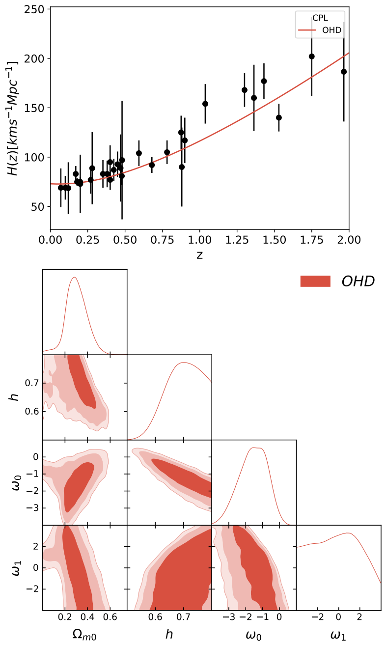
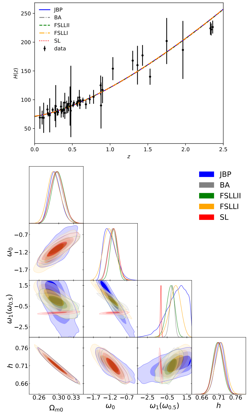
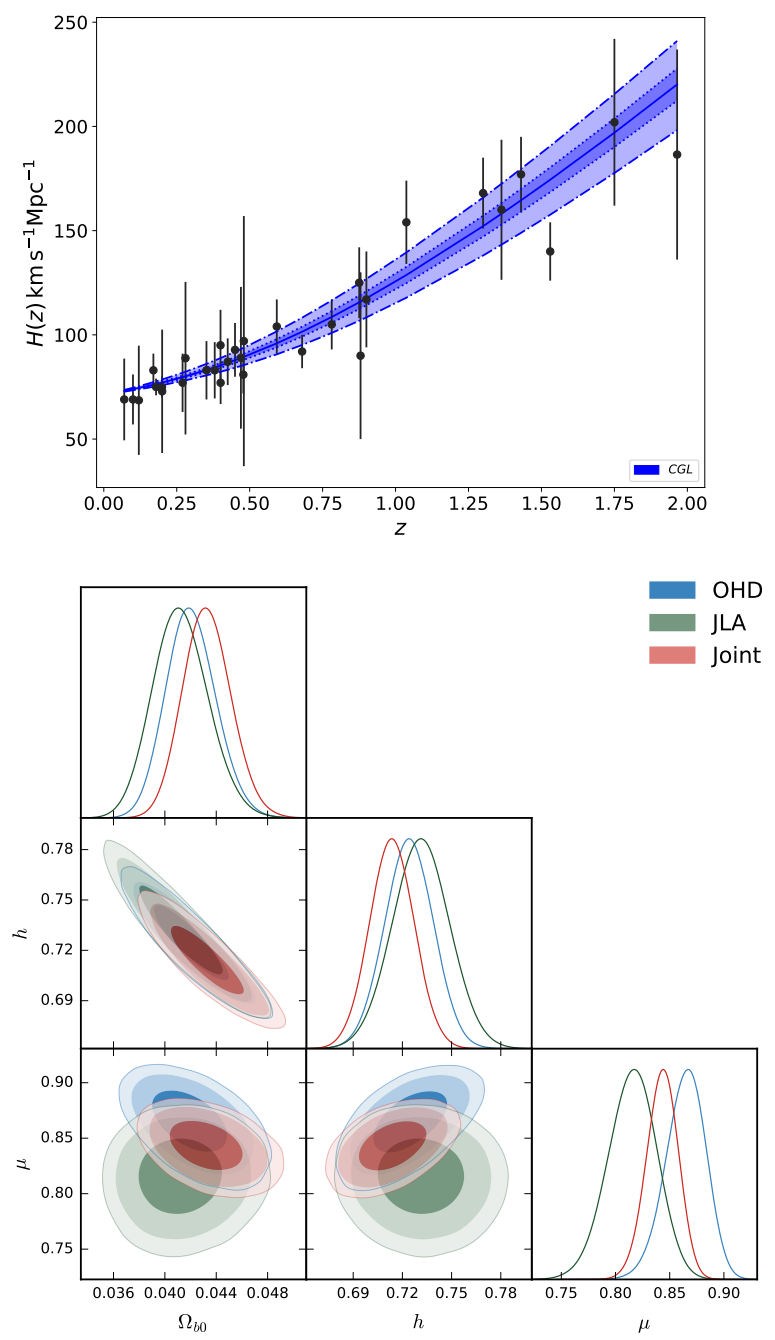
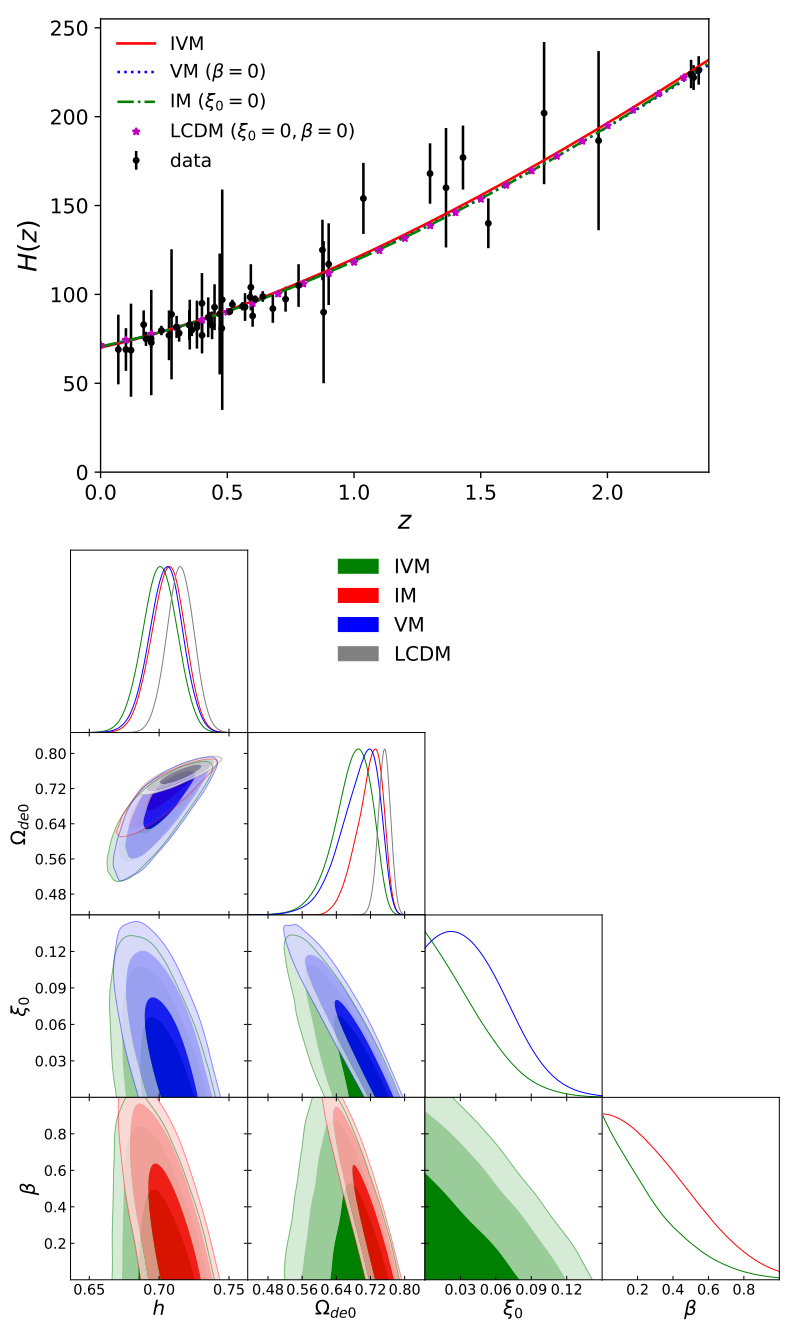
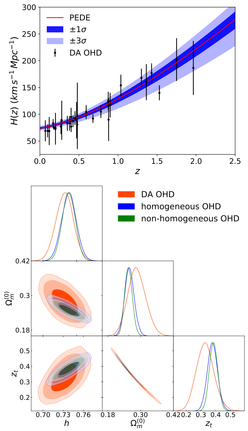
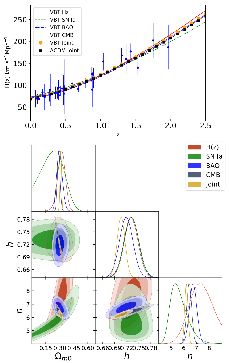
Table 1.
Mean values for the CDM parameters using the samples OHD, SNIa, CMB (Planck), and the joint of them.
Table 1.
Mean values for the CDM parameters using the samples OHD, SNIa, CMB (Planck), and the joint of them.
| Data | ||||
| OHD | ||||
| SNIa | ||||
| CMB | ||||
| Joint | ||||
Table 2.
Mean values for the , , and parameters using the joint analysis of OHD, CMB, and BAO data for the JBP, BA, FSLLI, FSLLII, and SL DE parameterizations (see [120]).
Table 2.
Mean values for the , , and parameters using the joint analysis of OHD, CMB, and BAO data for the JBP, BA, FSLLI, FSLLII, and SL DE parameterizations (see [120]).
| DE Parametrizations | |||||
|---|---|---|---|---|---|
| Model | |||||
| JBP | |||||
| BA | |||||
| FSLLI | |||||
| FSLLII | |||||
| SL | |||||
Table 3.
Mean values for the model parameters (, h, ) derived from OHD and SNIa measurements for a flat universe (see [131]).
Table 3.
Mean values for the model parameters (, h, ) derived from OHD and SNIa measurements for a flat universe (see [131]).
| Data Set | OHD | JLA | Joint |
|---|---|---|---|
| h | |||
| a | - | ||
| b | - | ||
| - | |||
| - |
Table 4.
Best fitting parameters of the polynomial model (see [134] for details).
Table 4.
Best fitting parameters of the polynomial model (see [134] for details).
| Data | n | h | ||||
|---|---|---|---|---|---|---|
| OHD | - | |||||
| SNIa | ||||||
| OHD+SNIa |
Table 5.
Best fitting parameters of the hyperbolic models (see [134] for details).
Table 5.
Best fitting parameters of the hyperbolic models (see [134] for details).
| Tanh Model | |||||
|---|---|---|---|---|---|
| Data | b | n | h | ||
| OHD | - | ||||
| SNIa | |||||
| OHD+SNIa | |||||
| Cosh Model | |||||
| Data | b | n | h | ||
| OHD | - | ||||
| SNIa | |||||
| OHD+SNIa | |||||
Table 6.
Best fitting values of the free model parameters (see [135] for details).
Table 6.
Best fitting values of the free model parameters (see [135] for details).
| Sample | h | |||||
|---|---|---|---|---|---|---|
| OHD | – | – | ||||
| SNIa | – | |||||
| SLS | – | – | ||||
| Joint | – | |||||
| OHD | – | |||||
| SNIa | ||||||
| SLS | – | |||||
| Joint | ||||||
Table 7.
Best fit values for the free parameters of IVM, IM, VM, and LCDM models using the OHD sample. The uncertainties are at (see [65] for details).
Table 7.
Best fit values for the free parameters of IVM, IM, VM, and LCDM models using the OHD sample. The uncertainties are at (see [65] for details).
| Model | h | ||||
|---|---|---|---|---|---|
| IVM | |||||
| IM | 0 | ||||
| VM | 0 | ||||
| LCDM | 0 | 0 |
Table 8.
Mean values of the free parameters for the PEDE model using homogeneous, non-homogeneous and DA OHD and a Gaussian prior on [32]. The last column shows the estimated redsfhit using the condition (see [39], for details). The uncertainties reported correspond to confidence level. In parenthesis are the best fit values when a flat prior on h is considered in the region .
| Sample | h | ||||
|---|---|---|---|---|---|
| PEDE | |||||
| homogeneous OHD | () | () | () | 0 | |
| non-homogeneous OHD | () | () | () | 0 | |
| DA OHD | () | () | () | 0 | |
Table 9.
Mean values of the free parameters for GEDE model using homogeneous, non-homogeneous and DA OHD and a Gaussian prior on [32]. The last column shows the estimated redsfhit using the condition (see [39] for details). The uncertainties reported correspond to confidence level. In parenthesis are the best fit values when a flat prior on h is considered in the region .
| Sample | h | ||||
|---|---|---|---|---|---|
| GEDE | |||||
| homogeneous OHD | () | () | () | () | () |
| non-homogeneous OHD | () | () | () | () | () |
| DA OHD | () | () | () | () | () |
Table 10.
Best fitting values of the free parameters for the constant brane tension model with the different samples used in this paper.
Table 10.
Best fitting values of the free parameters for the constant brane tension model with the different samples used in this paper.
| Sample | h | ||||
|---|---|---|---|---|---|
| OHD | <−0.88 | ||||
| BAO | <−9.52 | ||||
| SNIa | <−0.31 | ||||
| CMB | <−15.0 | ||||
| Joint | <−16.2 |
Table 11.
Best fitting values of the free parameters for the Variable Brane Tension model with the different samples used in this paper.
Table 11.
Best fitting values of the free parameters for the Variable Brane Tension model with the different samples used in this paper.
| Sample | h | n | eV | ||
|---|---|---|---|---|---|
| OHD | |||||
| BAO | |||||
| SNIa | |||||
| CMB | |||||
| Joint |
Table 12.
Mean values for the UG model parameters (h, ) and , derived from each data set and the joint analysis (see [97]).
Table 12.
Mean values for the UG model parameters (h, ) and , derived from each data set and the joint analysis (see [97]).
| Sample | h | ||
|---|---|---|---|
| OHD | |||
| SnIa | |||
| CMB | |||
| BAO | |||
| Joint |
Table 13.
Best fitting values of the free parameters for the EGB model with the different samples used in this paper (see [47] for details).
Table 13.
Best fitting values of the free parameters for the EGB model with the different samples used in this paper (see [47] for details).
| Sample | h | ||||
|---|---|---|---|---|---|
| OHD | – | ||||
| BAO | – | ||||
| SNIa | |||||
| SLS | – | ||||
| HIIG | – | ||||
| Joint |
Table 14.
Mean values for the OC and MPC parameters using the samples OHD (DA), SNIa (compressed JLA), and the joint analysis of these data sets. (see [66], for details).
Table 14.
Mean values for the OC and MPC parameters using the samples OHD (DA), SNIa (compressed JLA), and the joint analysis of these data sets. (see [66], for details).
| Orignal Cardassian | |||||
|---|---|---|---|---|---|
| Data | n | l | h | ||
| OHD (DA) | |||||
| SNIa | |||||
| Joint | |||||
| Modified polytropic Cardassian | |||||
| OHD (DA) | |||||
| SNIa | |||||
| Joint | |||||
Table 15.
Best fitting values of the h parameter for all the models presented.
| Model | h | Sample | Prior |
|---|---|---|---|
| wCDM | OHD, SNIa, CMB | Gaussian ( | |
| CPL | OHD | Flat [0.2,1.0] | |
| JBP | OHD, CMB, BAO | Gaussian () | |
| BA | OHD, CMB, BAO | Gaussian () | |
| FSLLI | OHD, CMB, BAO | Gaussian () | |
| FSLLII | OHD, CMB, BAO | Gaussian () | |
| SL | OHD, CMB, BAO | Gaussian () | |
| Chaplygin-Like Fluid | OHD, SNIa | Gaussian () | |
| Viscous (Polynomial) | OHD, SNIa | Gaussian () | |
| Viscous (Hyperbolic tanh) | OHD, SNIa | Gaussian () | |
| Viscous (Hyperbolic cosh) | OHD, SNIa | Gaussian () | |
| Viscous ( Constant) | OHD, SNIa, SLS | Gaussian () | |
| Viscous ( Polynomial) | OHD, SNIa, SLS | Gaussian () | |
| Interacting Viscous | OHD | Gaussian () | |
| PEDE | Homogeneous OHD | Gaussian () | |
| GEDE | Homogeneous OHD | Gaussian () | |
| CBT | BAO, SNIa, OHD, CMB | Gaussian () | |
| VBT | OHD, SNIa, BAO, BAO | Gaussian () | |
| UG | OHD, SNIa, CMB, BAO | Flat [0.2,1.0] | |
| EGB | SNIa, BAO, OHD, SLS, HIIG | Gaussian () | |
| Original Cardassian | SNIa, OHD | Flat [0,1] | |
| Modified Polytropic Cardassian | SNIa, OHD | Flat [0,1] |
Publisher’s Note: MDPI stays neutral with regard to jurisdictional claims in published maps and institutional affiliations. |
© 2021 by the authors. Licensee MDPI, Basel, Switzerland. This article is an open access article distributed under the terms and conditions of the Creative Commons Attribution (CC BY) license (https://creativecommons.org/licenses/by/4.0/).
Share and Cite
MDPI and ACS Style
Motta, V.; García-Aspeitia, M.A.; Hernández-Almada, A.; Magaña, J.; Verdugo, T. Taxonomy of Dark Energy Models. Universe 2021, 7, 163. https://0-doi-org.brum.beds.ac.uk/10.3390/universe7060163
AMA Style
Motta V, García-Aspeitia MA, Hernández-Almada A, Magaña J, Verdugo T. Taxonomy of Dark Energy Models. Universe. 2021; 7(6):163. https://0-doi-org.brum.beds.ac.uk/10.3390/universe7060163
Chicago/Turabian StyleMotta, Verónica, Miguel A. García-Aspeitia, Alberto Hernández-Almada, Juan Magaña, and Tomás Verdugo. 2021. "Taxonomy of Dark Energy Models" Universe 7, no. 6: 163. https://0-doi-org.brum.beds.ac.uk/10.3390/universe7060163
Note that from the first issue of 2016, this journal uses article numbers instead of page numbers. See further details here.