
Inclination Estimates from Off-Axis GRB Afterglow Modelling

 , , , , , , , , and
Abstract
:1. Introduction
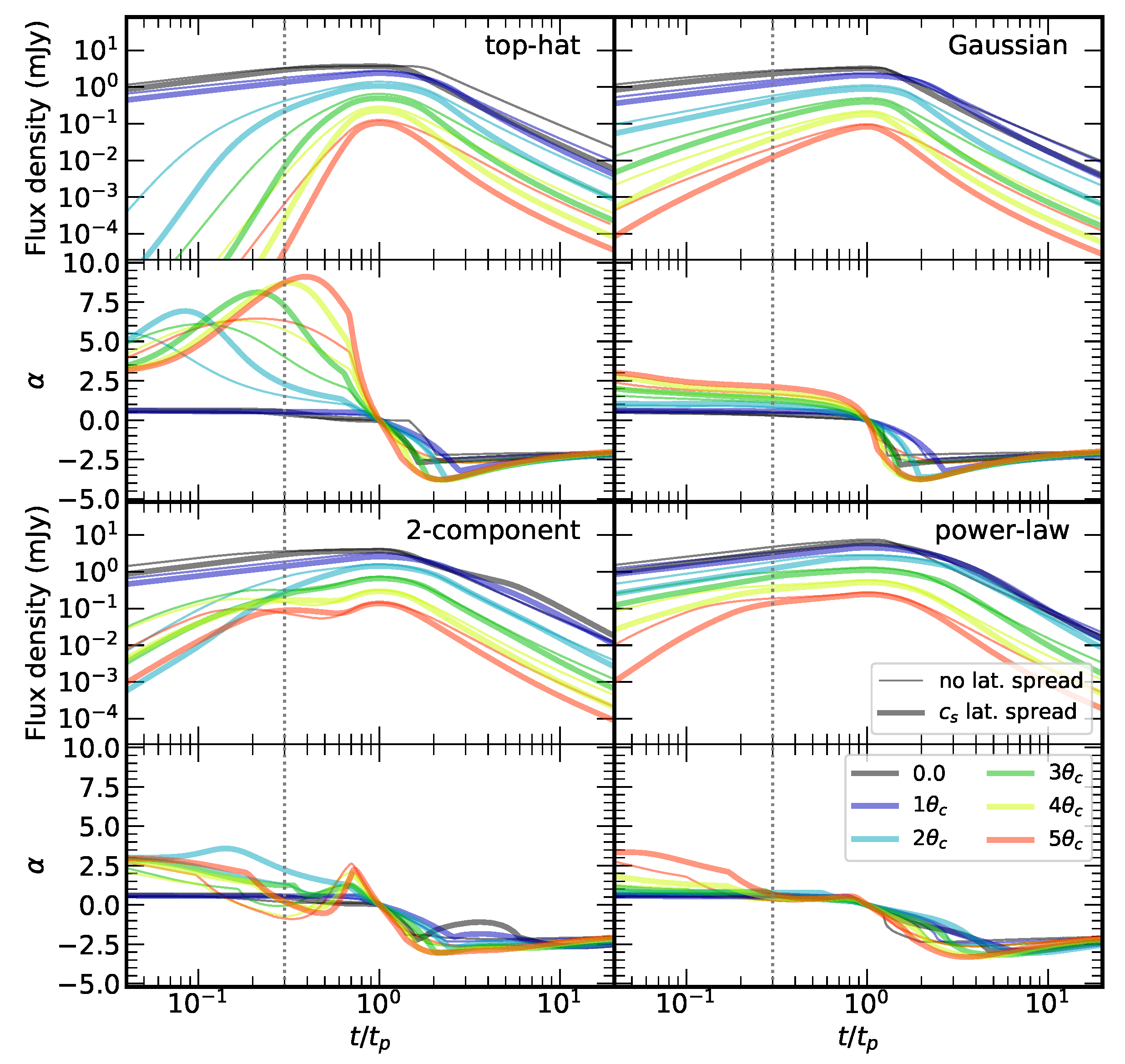
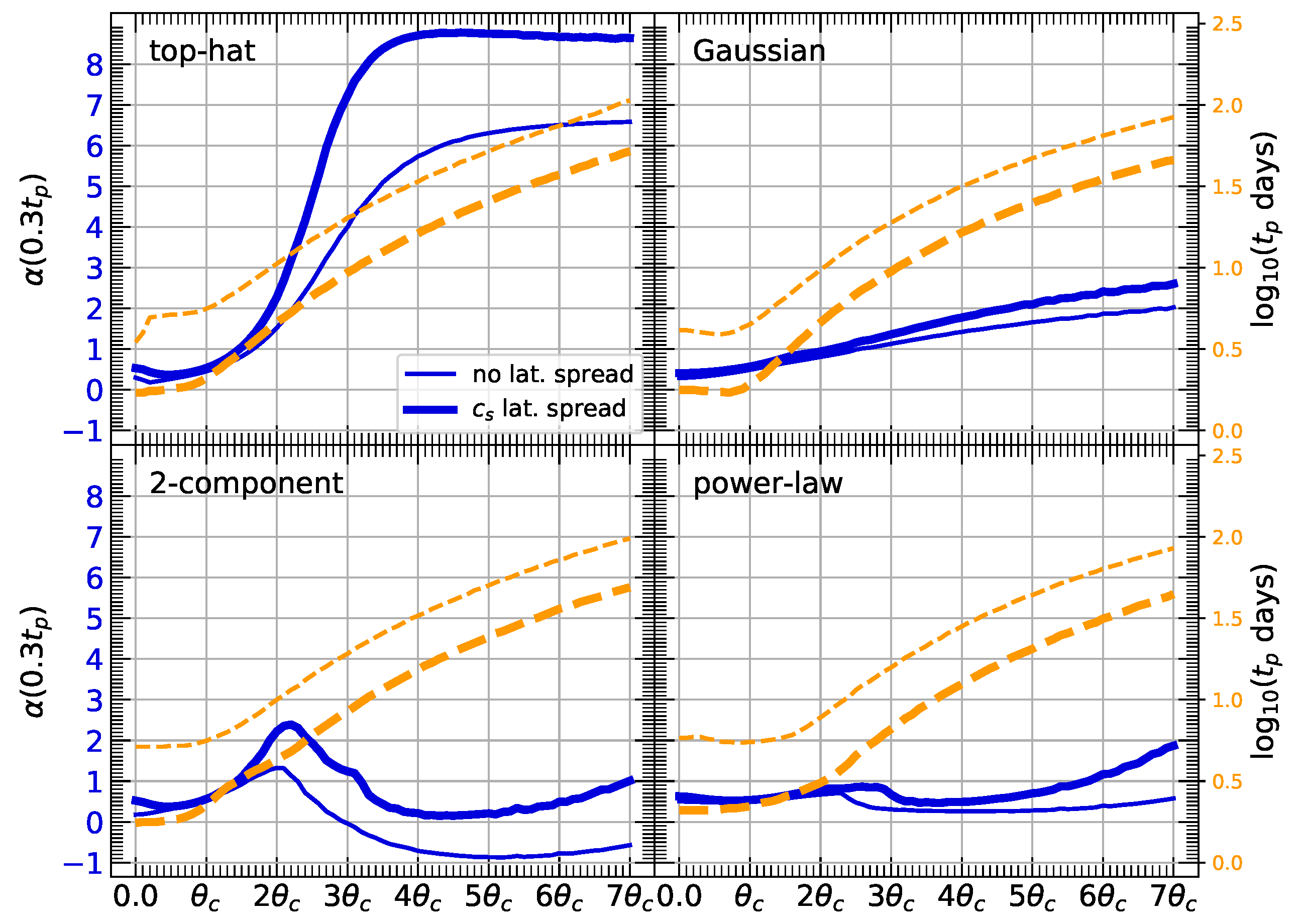
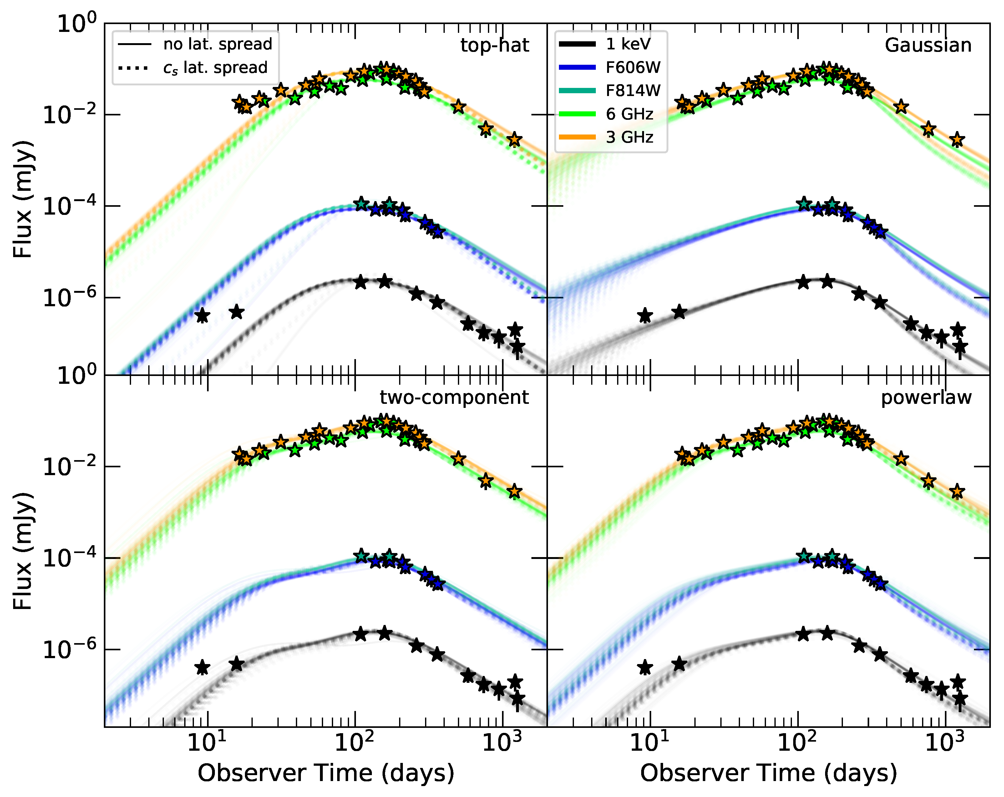
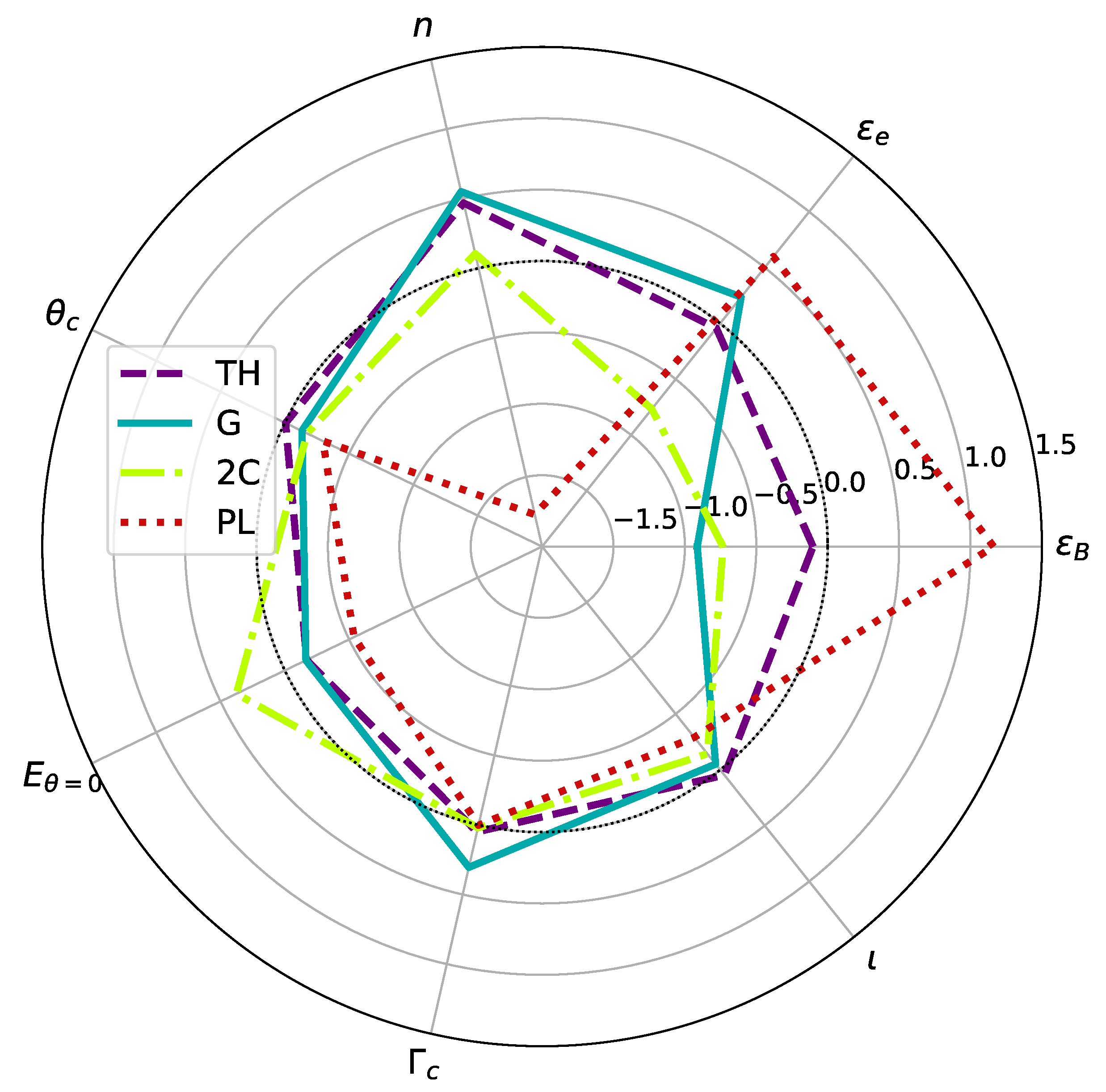
2. Method
- TH
- Top-hat: a uniform in isotropic-equivalent kinetic energy, E, and Lorentz factor, , with angle until a sharp edge at the jet opening angle, , where the energy goes to zero.
- G
- Gaussian: a jet profile described by a Gaussian function with , and .
- 2C
- Two-component: a top-hat jet surrounded by a wider uniform region of lower energy with , and .
- PL
- Powerlaw: a top-hat jet surrounded by a region where the energy and Lorentz factor declines with increasing angle as a powerlaw, , and .
3. Results
4. Discussion
5. Conclusions
Author Contributions
Funding
Institutional Review Board Statement
Informed Consent Statement
Data Availability Statement
Acknowledgments
Conflicts of Interest
Abbreviations
| GRB | Gamma ray burst |
| GW | Gravitational wave |
| EM | Electromagnetic |
| GW-EM | Gravitational waves and electromagnetic emission |
| TH | Top-hat |
| G | Gaussian |
| 2C | Two-component |
| PL | Powerlaw |
| MCMC | Markov chain monte carlo |
| w | With |
| wo | Without |
| VLBI | Very long baseline interferometry |
| GHz | Giga-Hertz |
| STFC | Science technology and facilities council |
| 1 |
References
- Nakar, E. The electromagnetic counterparts of compact binary mergers. Phys. Rev. 2020, 886, 1–84. [Google Scholar] [CrossRef]
- Lamb, G.P.; Kobayashi, S. Electromagnetic counterparts to structured jets from gravitational wave detected mergers. Mon. Not. R. Astron. Soc. 2017, 472, 4953–4964. [Google Scholar] [CrossRef]
- Lazzati, D.; Deich, A.; Morsony, B.J.; Workman, J.C. Off-axis emission of short γ-ray bursts and the detectability of electromagnetic counterparts of gravitational-wave-detected binary mergers. Mon. Not. R. Astron. Soc. 2017, 471, 1652–1661. [Google Scholar] [CrossRef] [Green Version]
- Jin, Z.P.; Li, X.; Wang, H.; Wang, Y.Z.; He, H.N.; Yuan, Q.; Zhang, F.W.; Zou, Y.C.; Fan, Y.Z.; Wei, D.M. Short GRBs: Opening Angles, Local Neutron Star Merger Rate, and Off-axis Events for GRB/GW Association. Astrophys. J. 2018, 857, 128. [Google Scholar] [CrossRef]
- Kathirgamaraju, A.; Barniol Duran, R.; Giannios, D. Off-axis short GRBs from structured jets as counterparts to GW events. Mon. Not. R. Astron. Soc. 2018, 473, L121–L125. [Google Scholar] [CrossRef]
- Wang, H.; Giannios, D. Multimessenger Parameter Estimation of GW170817: From Jet Structure to the Hubble Constant. Astrophys. J. 2021, 908, 200. [Google Scholar] [CrossRef]
- Hotokezaka, K.; Nakar, E.; Gottlieb, O.; Nissanke, S.; Masuda, K.; Hallinan, G.; Mooley, K.P.; Deller, A.T. A Hubble constant measurement from superluminal motion of the jet in GW170817. Nat. Astron. 2019, 3, 940–944. [Google Scholar] [CrossRef] [Green Version]
- Mastrogiovanni, S.; Duque, R.; Chassande-Mottin, E.; Daigne, F.; Mochkovitch, R. What role will binary neutron star merger afterglows play in multimessenger cosmology? arXiv 2020, arXiv:2012.12836. [Google Scholar]
- Van Eerten, H.; van der Horst, A.; MacFadyen, A. Gamma-Ray Burst Afterglow Broadband Fitting Based Directly on Hydrodynamics Simulations. Astrophys. J. 2012, 749, 44. [Google Scholar] [CrossRef] [Green Version]
- Granot, J.; Piran, T. On the lateral expansion of gamma-ray burst jets. Mon. Not. R. Astron. Soc. 2012, 421, 570–587. [Google Scholar] [CrossRef] [Green Version]
- Fernández, J.J.; Kobayashi, S.; Lamb, G.P. Determining the viewing angle of neutron star merger jets with VLBI radio images. arXiv 2021, arXiv:2101.05138. [Google Scholar]
- Huang, Y.F.; Gou, L.J.; Dai, Z.G.; Lu, T. Overall Evolution of Jetted Gamma-Ray Burst Ejecta. Astrophys. J. 2000, 543, 90–96. [Google Scholar] [CrossRef] [Green Version]
- Lamb, G.P.; Kann, D.A.; Fernández, J.J.; Mandel, I.; Levan, A.J.; Tanvir, N.R. GRB jet structure and the jet break. arXiv 2021, arXiv:2104.11099. [Google Scholar]
- Lamb, G.P.; Kobayashi, S. GRB 170817A as a jet counterpart to gravitational wave triggerGW 170817. Mon. Not. R. Astron. Soc. 2018, 478, 733–740. [Google Scholar] [CrossRef] [Green Version]
- Lamb, G.P.; Mandel, I.; Resmi, L. Late-time evolution of afterglows from off-axis neutron star mergers. Mon. Not. R. Astron. Soc. 2018, 481, 2581–2589. [Google Scholar] [CrossRef] [Green Version]
- Lyman, J.D.; Lamb, G.P.; Levan, A.J.; Mandel, I.; Tanvir, N.R.; Kobayashi, S.; Gompertz, B.; Hjorth, J.; Fruchter, A.S.; Kangas, T.; et al. The optical afterglow of the short gamma-ray burst associated with GW170817. Nat. Astron. 2018, 2, 751–754. [Google Scholar] [CrossRef]
- Lamb, G.P.; Lyman, J.D.; Levan, A.J.; Tanvir, N.R.; Kangas, T.; Fruchter, A.S.; Gompertz, B.; Hjorth, J.; Mandel, I.; Oates, S.R.; et al. The Optical Afterglow of GW170817 at One Year Post-merger. Astrophys. J. Lett. 2019, 870, L15. [Google Scholar] [CrossRef] [Green Version]
- Lamb, G.P.; Kobayashi, S. Reverse shocks in the relativistic outflows of gravitational wave-detected neutron star binary mergers. Mon. Not. R. Astron. Soc. 2019, 489, 1820–1827. [Google Scholar] [CrossRef]
- Lamb, G.P.; Levan, A.J.; Tanvir, N.R. GRB 170817A as a Refreshed Shock Afterglow Viewed Off-axis. Astrophys. J. 2020, 899, 105. [Google Scholar] [CrossRef]
- Richardson, L.F. IX. The approximate arithmetical solution by finite differences of physical problems involving differential equations, with an application to the stresses in a masonry dam. Philos. Trans. R. Soc. Lond. Ser. A Contain. Pap. Math. Phys. Character 1911, 210, 307–357. [Google Scholar]
- Troja, E.; O’Connor, B.; Ryan, G.; Piro, L.; Ricci, R.; Zhang, B.; Piran, T.; Bruni, G.; Cenko, S.B.; van Eerten, H. Accurate flux calibration of GW170817: Is the X-ray counterpart on the rise? arXiv 2021, arXiv:2104.13378. [Google Scholar]
- Balasubramanian, A.; Corsi, A.; Mooley, K.P.; Brightman, M.; Hallinan, G.; Hotokezaka, K.; Kaplan, D.L.; Lazzati, D.; Murphy, E.J. Continued Radio Observations of GW170817 3.5 yr Post-merger. Astrophys. J. Lett. 2021, 914, L20. [Google Scholar] [CrossRef]
- Makhathini, S.; Mooley, K.P.; Brightman, M.; Hotokezaka, K.; Nayana, A.; Intema, H.T.; Dobie, D.; Lenc, E.; Perley, D.A.; Fremling, C.; et al. The Panchromatic Afterglow of GW170817: The full uniform dataset, modeling, comparison with previous results and implications. arXiv 2020, arXiv:2006.02382. [Google Scholar]
- Fong, W.; Blanchard, P.K.; Alexander, K.D.; Strader, J.; Margutti, R.; Hajela, A.; Villar, V.A.; Wu, Y.; Ye, C.S.; Berger, E.; et al. The Optical Afterglow of GW170817: An Off-axis Structured Jet and Deep Constraints on a Globular Cluster Origin. Astrophys. J. Lett. 2019, 883, L1. [Google Scholar] [CrossRef] [Green Version]
- Troja, E.; Piro, L.; Ryan, G.; van Eerten, H.; Ricci, R.; Wieringa, M.H.; Lotti, S.; Sakamoto, T.; Cenko, S.B. The outflow structure of GW170817 from late-time broad-band observations. Mon. Not. R. Astron. Soc. 2018, 478, L18–L23. [Google Scholar] [CrossRef]
- Foreman-Mackey, D.; Hogg, D.W.; Lang, D.; Goodman, J. emcee: The MCMC Hammer. PASP 2013, 125, 306. [Google Scholar] [CrossRef] [Green Version]
- Gill, R.; Granot, J.; De Colle, F.; Urrutia, G. Numerical Simulations of an Initially Top-hat Jet and the Afterglow of GW170817/GRB170817A. Astrophys. J. 2019, 883, 15. [Google Scholar] [CrossRef] [Green Version]
- Lazzati, D.; Perna, R.; Morsony, B.J.; Lopez-Camara, D.; Cantiello, M.; Ciolfi, R.; Giacomazzo, B.; Workman, J.C. Late Time Afterglow Observations Reveal a Collimated Relativistic Jet in the Ejecta of the Binary Neutron Star Merger GW170817. Phys. Rev. Lett. 2018, 120, 241103. [Google Scholar] [CrossRef] [Green Version]
- Margutti, R.; Alexander, K.D.; Xie, X.; Sironi, L.; Metzger, B.D.; Kathirgamaraju, A.; Fong, W.; Blanchard, P.K.; Berger, E.; MacFadyen, A.; et al. The Binary Neutron Star Event LIGO/Virgo GW170817 160 Days after Merger: Synchrotron Emission across the Electromagnetic Spectrum. Astrophys. J. Lett. 2018, 856, L18. [Google Scholar] [CrossRef] [Green Version]
- Resmi, L.; Schulze, S.; Ishwara-Chandra, C.H.; Misra, K.; Buchner, J.; De Pasquale, M.; Sánchez-Ramírez, R.; Klose, S.; Kim, S.; Tanvir, N.R.; et al. Low-frequency View of GW170817/GRB 170817A with the Giant Metrewave Radio Telescope. Astrophys. J. 2018, 867, 57. [Google Scholar] [CrossRef] [Green Version]
- Nakar, E.; Piran, T. Afterglow Constraints on the Viewing Angle of Binary Neutron Star Mergers and Determination of the Hubble Constant. Astrophys. J. 2021, 909, 114. [Google Scholar] [CrossRef]
- Granot, J.; Sari, R. The Shape of Spectral Breaks in Gamma-Ray Burst Afterglows. Astrophys. J. 2002, 568, 820–829. [Google Scholar] [CrossRef] [Green Version]
- Gao, H.; Lei, W.H.; Zou, Y.C.; Wu, X.F.; Zhang, B. A complete reference of the analytical synchrotron external shock models of gamma-ray bursts. New Astron. Rev. 2013, 57, 141–190. [Google Scholar] [CrossRef] [Green Version]
- Resmi, L.; Zhang, B. Gamma-ray Burst Reverse Shock Emission in Early Radio Afterglows. Astrophys. J. 2016, 825, 48. [Google Scholar] [CrossRef] [Green Version]
- Ryan, G.; van Eerten, H.; Piro, L.; Troja, E. Gamma-Ray Burst Afterglows in the Multimessenger Era: Numerical Models and Closure Relations. Astrophys. J. 2020, 896, 166. [Google Scholar] [CrossRef]
- Ghirlanda, G.; Salafia, O.S.; Paragi, Z.; Giroletti, M.; Yang, J.; Marcote, B.; Blanchard, J.; Agudo, I.; An, T.; Bernardini, M.G.; et al. Compact radio emission indicates a structured jet was produced by a binary neutron star merger. Science 2019, 363, 968–971. [Google Scholar] [CrossRef] [Green Version]
- Mooley, K.P.; Deller, A.T.; Gottlieb, O.; Nakar, E.; Hallinan, G.; Bourke, S.; Frail, D.A.; Horesh, A.; Corsi, A.; Hotokezaka, K. Superluminal motion of a relativistic jet in the neutron-star merger GW170817. Nature 2018, 561, 355–359. [Google Scholar] [CrossRef]
- Salafia, O.S.; Barbieri, C.; Ascenzi, S.; Toffano, M. Gamma-ray burst jet propagation, development of angular structure, and the luminosity function. A&A 2020, 636, A105. [Google Scholar] [CrossRef]
- Murguia-Berthier, A.; Ramirez-Ruiz, E.; De Colle, F.; Janiuk, A.; Rosswog, S.; Lee, W.H. The Fate of the Merger Remnant in GW170817 and Its Imprint on the Jet Structure. Astrophys. J. 2021, 908, 152. [Google Scholar] [CrossRef]


| Units | [log cm] | [rad] | [log erg] | |||||
|---|---|---|---|---|---|---|---|---|
| Prior | – | – | –2 | – | 48–55 | 6–600 | – | |
| TH | wo | |||||||
| w | ||||||||
| G | wo | |||||||
| w | ||||||||
| 2C | wo | |||||||
| w | ||||||||
| PL | wo | |||||||
| w | ||||||||
Publisher’s Note: MDPI stays neutral with regard to jurisdictional claims in published maps and institutional affiliations. |
© 2021 by the authors. Licensee MDPI, Basel, Switzerland. This article is an open access article distributed under the terms and conditions of the Creative Commons Attribution (CC BY) license (https://creativecommons.org/licenses/by/4.0/).
Share and Cite
Lamb, G.P.; Fernández, J.J.; Hayes, F.; Kong, A.K.H.; Lin, E.-T.; Tanvir, N.R.; Hendry, M.; Heng, I.S.; Saha, S.; Veitch, J. Inclination Estimates from Off-Axis GRB Afterglow Modelling. Universe 2021, 7, 329. https://0-doi-org.brum.beds.ac.uk/10.3390/universe7090329
Lamb GP, Fernández JJ, Hayes F, Kong AKH, Lin E-T, Tanvir NR, Hendry M, Heng IS, Saha S, Veitch J. Inclination Estimates from Off-Axis GRB Afterglow Modelling. Universe. 2021; 7(9):329. https://0-doi-org.brum.beds.ac.uk/10.3390/universe7090329
Chicago/Turabian StyleLamb, Gavin P., Joseph J. Fernández, Fergus Hayes, Albert K. H. Kong, En-Tzu Lin, Nial R. Tanvir, Martin Hendry, Ik Siong Heng, Surojit Saha, and John Veitch. 2021. "Inclination Estimates from Off-Axis GRB Afterglow Modelling" Universe 7, no. 9: 329. https://0-doi-org.brum.beds.ac.uk/10.3390/universe7090329