Inflationary Implications of the Covariant Entropy Bound and the Swampland de Sitter Conjectures

Abstract

We present a proposal to relate the de Sitter conjecture (dSC) with the time dependence of fluxes via the covariant entropy bound (CEB). By assuming an early phase of accelerated expansion where the CEB is satisfied, we take into account a contribution from time-dependent flux compactification to the four-dimensional entropy which establishes a bound on the usual slow-roll parameters ${\eta }_H$ and ${ϵ}_H$. We also show an explicit calculation of entropy from a toroidal flux compactification, from a transition amplitude of time-dependent fluxes which allows us to determine the conditions on which the bounds on the slow-roll parameters are in agreement to the dSC.

1. Introduction

The Swampland program has reached great advances in the last few years in its pursuit of characterize those features distinguishing effective theories that can be consistently completed into a quantum gravity theory (Landscape) from those which do not (Swampland) [1,2,3,4]. The boundary between the Landscape and Swampland is usually defined by a series of bounds on quantities of the proper effective theory which, in turn, are expressed in terms of the Planck mass $M_p$. In the limit where gravity decouples, i.e., $M_p\to \infty$, the Swampland constraints vanish. A question to be answered is whether these boundaries can be traced back to some essential microscopic physics in the Quantum Gravity Theory, or accordingly, to some fundamental constraints in the 10-dimensional String Theory formulation.

Many different bounds have been proposed as Swampland conjectures, although it is expected that all of them are related in some way through more fundamental principles (see review [3] and lectures [4] for references). Some of them are based on solid grounds, such as the distance conjecture and the weak gravity conjecture, while others, as the de Sitter conjectures, were initially motivated by some empirical evidence based on string models [5,6], and appropriately refined into its final form in order to be compatible with some well known effective scenarios such as the Higgs potential [7] among others. The refined version of the conjecture was motivated by stability of de Sitter extrema [8], by cosmological arguments through the slow-roll parameter ${\eta }_V$ [9], as well as by entropy arguments together with the distance conjecture on the dS space [10]. Many logic and solid arguments have been followed in the literature [11,12,13,14,15,16,17,18,19,20] so far with the purpose to give stronger ground basis to this conjecture. A matter of particular interest to us is the series of arguments supporting the de Sitter conjecture (dSC) based on the laws of thermodynamics [21,22,23,24]. Relating the dSC to thermodynamic principles, such as a positive temperature phase and the concavity of the entropy functional, respectively, have also been considered in the literature. Furthermore, as stochastic effects become relevant, it is found by thermodynamic arguments that slow-roll conditions either violate the second law or the swampland dSC [25,26].

In its original form, the de Sitter conjecture states that

$$\begin{array}{c}\hfill \frac{|\nabla V|}{V}\ge c\mathrm{or}\frac{\min {\nabla }_i{\partial }_{j}V}{V}\le -c^{\prime },\end{array}$$

(1)

with c and $c^{\prime }$ positive constants of order one in Planck units and V the effective scalar field potential. In addition to the well known implication of discarding the existence of dS minima, dSC also have implications on single and multi-field inflationary scenarios [27,28] which have been proven to be a matter of great interest [29,30,31,32,33,34,35,36,37,38,39,40,41].

In this paper, we are interested in studying the implications of the CEB [42,43,44,45] on the inflationary slow-roll parameters. We shall show that a time dependence of entropy (which in turn we propose it comes from a time-dependent flux compactification) leads to the presence of bounds on ${\eta }_H$ and ${ϵ}_H$. Our goal is to determine if such bounds are related to the dSC inequalities.

However, it is important to emphasize that we are not generating an expanding (inflationary or not) four-dimensional Universe through fluxes. The source of an expanding Universe from a string theory point of view is beyond the scope of this paper. Our interest focuses on the compatibility of an inflationary Universe with the CEB1.

The paper is organized as follows. In Section 2, we briefly review some basics regarding the CEB and establish a relation between the change of entropy over time and the slow-roll parameter ${ϵ}_H$ Equation (9). In Section 3, we use this relation to study its implications on single field and multi-field inflationary scenarios. Our main result is that we are able to reproduce the inequalities of the dSC, as well as the mutual exclusion between them in terms of the time variation of entropy sourced from physics in extra dimensions, as well as the explicit form of the constants c and $c^{\prime }$ in terms of entropy and time derivatives of it. A simple example concerning a toroidal flux compactification is presented to show how fluxes contribute to the four-dimensional entropy. Finally, we discuss our conclusions and some final comments.

2. Covariant Entropy Bound and Inflation 2

The covariant entropy bound (CEB) is a well tested conjecture in many gravitationally scenarios, including cosmology [42,43,44,45]. Basically, it states that for a codimension 2 surface B, there exist at least two light-sheets L, defined as the codimension 1 null hypersurfaces orthogonal to B spanned by light-type trajectories terminating at a singularity or a caustic, with a negative expansion rate. These light-sheets can be future or past-directed. The general statement is that the entropy associated to the light-sheet $S\left(L\right[B\left]\right)$, at a given time, is bounded by the area A of the surface B as2

$$S\left(L\left[B\right]\right)\le \frac{A\left(B\right)}{4}.$$

(2)

In [10] the association of the CEB with an expanding de Sitter (dS) Universe establishes a bound for the entropy given by,

$$S\le \pi R_{AH}^2,$$

(3)

where $R_{AH}$ is the radius of the apparent horizon (AH). Appealing to the distance conjecture (DC), it is discussed the case in which entropy increases with the field moduli distance through the appearance of towers of massless modes $\varphi$. Since in a dS space $R_{AH}^2\sim 1/V$, where V is the scalar potential, the CEB implies that3

$${\partial }_{\varphi }S\le -\frac{{\partial }_{\varphi }V}{V^2}.$$

(4)

Due to the fact that the potential V decreases as the number of massless modes grows, ${\partial }_{\varphi }V<0$. By taking ${\partial }_{\varphi }S\sim c/V$, with c a number of order 1 in Planck units, the slow-roll parameter ${ϵ}_V$ acquires a bound given by

$$2{ϵ}_V=\frac{|{\partial }_{\varphi }{V|}^2}{{\left|V\right|}^2}\ge c^2.$$

(5)

As noticed in [9], ${ϵ}_V$ is not necessarily of order 1 if

$${\eta }_V\le -c^{\prime },$$

(6)

with $c^{\prime }$ another constant of order 1 in Planck Units. This was also concluded in [10] by constraining the scalar potential fluctuations to remain within the AH. In this context, the refined de Sitter conjecture (dSC) follows from the dependence of entropy, and of the apparent horizon radius, on the tower of massless modes.

In this work we are interested in a slightly different—but equivalent—approach by demanding that entropy and $R_{AH}$ increases as time runs, via an effective scalar field $\varphi$ derived from a string compactification with fluxes depending on time.

We now proceed to elaborate our proposal. In a flat 4-dimensional expanding Universe described by the Friedmann–Robertson–Walker (FRW) metric:

$$\begin{array}{c}\hfill d{s}_4^2=-d{t}^2+a^2\left(t\right)(d{r}^2+r^{2}d{\Omega }^2),\end{array}$$

(7)

It is possible to define the radius of the AH at a time t as $R_{AH}=1/H$, with H the Hubble constant defined as $H=\dot{a}/a$, where $\dot{a}$ denotes the time derivative with respect to the proper time t. As the Universe expands, the comoving Hubble radius $R_{AH}/a$ shrinks and the AH comoving area given by

$$A_{AH}=4\pi R_{AH}^2=\frac{4{\pi }^2}{H^2}$$

(8)

increases. Following [45], an infinitesimal variation of time helps us to rewrite the CEB in the form4.

$$\gamma \equiv \frac{H\dot{S}}{2\pi }\le {ϵ}_H,$$

(9)

with ${ϵ}_H=-\dot{H}/H^2$ the usual slow-roll inflationary parameter satisfying ${ϵ}_H\ll 1$, implying that ${\dot{\varphi }}^2$ and $\ddot{\varphi }$ are much smaller than V. Notice that according to our anzatz, as the AH radius increases we also expect an increase on entropy, thus our model is valid only for $\dot{S}>0$.

In the following we shall assume that a variation of entropy in time comes from extra dimensions within a string theory based scenario. In this context, we expect that entropy must be a function of the Hubble parameter H, time and other string parameters which we shall ignore to our present purpose.

3. Inflation and Effective Field Theory

Let us consider an N-field scenario. As shown in [57], it is more convenient to switch to the kinematic −Frenet–Serret− frame to compute the equations of motion of an effective theory in the presence of a scalar potential $V=V\left({\varphi }_a\right)$ with $a=1,\dots N$. See Appendix A for more details.

The equations of motion can be written in terms of the unitary tangential vector ${\widehat{e}}_1$, the normal ${\widehat{e}}_2$ and the $(N-2)$ binormal ${\widehat{e}}_i$, as

$$(\ddot{\varphi }+3H\dot{\varphi }+V_1){\widehat{e}}_1+(-\dot{\varphi }{\Omega }_1+V_2){\widehat{e}}_2+V_i{\widehat{e}}_i=0,$$

(10)

with $i=3,\dots ,N$, $\dot{\varphi }$ is the norm of the vector field $\overrightarrow{\dot{\varphi }}=({\dot{\varphi }}^1,\dots ,{\dot{\varphi }}^n)$ and ${\Omega }_1$ is the curvature defined as $D_t{\widehat{e}}_1=-{\Omega }_1{\widehat{e}}_2$. Since the Frenet–Serret frame $\{{\widehat{e}}_1,{\widehat{e}}_2,{\widehat{e}}_i\}$ is an orthonormal basis, we find that

$$\begin{array}{ccc}\hfill \ddot{\varphi }+3H\dot{\varphi }+V_1& =& 0,\hfill \end{array}$$

(11)

$$\begin{array}{ccc}\hfill -\dot{\varphi }{\Omega }_1+V_2& =& 0,\hfill \end{array}$$

(12)

$$\begin{array}{ccc}\hfill V_i& =& 0.\hfill \end{array}$$

(13)

Notice all projections of $\overrightarrow{\nabla }V$ along normal vectors ${\widehat{e}}_i$, denoted by $V_i$, vanish for $i=3,\dots ,n$, implying that we can focus only on the field trajectory on the osculating plane.

Now, together with the Einstein–Friedmann equation

$$\begin{array}{c}\hfill 3H^2=\frac{{\dot{\varphi }}^2}{2}+V,\end{array}$$

(14)

and by the usual definitions of the slow-roll parameters,

$$\begin{array}{c}\hfill {ϵ}_V\equiv \frac{1}{2}{\left(\frac{\overrightarrow{\nabla }V}{V}\right)}^2={\widetilde{ϵ}}_V+{\widehat{ϵ}}_V,\end{array}$$

(15)

with

$${\widetilde{ϵ}}_V=\frac{1}{2}{\left(\frac{V_1}{V}\right)}^2,{\widehat{ϵ}}_V=\frac{1}{2}{\left(\frac{V_2}{V}\right)}^2,$$

(16)

we can construct a relation between ${ϵ}_H$ and ${\widehat{ϵ}}_V$ given by

$${ϵ}_H^2-(6+\alpha ){ϵ}_H+9=0,$$

(17)

where

$$\begin{array}{c}\hfill \alpha =\frac{{\Omega }_1^2}{H^2{\widehat{ϵ}}_V}=\frac{2V^2}{H^2{\dot{\varphi }}^2},\end{array}$$

(18)

with ${\widehat{ϵ}}_V\ne 0$. Notice that $\alpha \to 0$ implies ${ϵ}_H\to 3$ for which an accelerated expansion—and therefore inflation—is ruled out. An almost zero $\alpha$ means two things: one is that the kinetic energy is much bigger than V; the second possibility involves ${\widehat{ϵ}}_V$ growing faster than the ratio ${\Omega }_1/H$.

By using ${ϵ}_H$ as a function of ${\widehat{ϵ}}_V$ from (17) we obtain from inequality (9)

$$\begin{array}{ccc}\hfill \gamma & \le & \left(3+\frac{\alpha }{2}\right)\pm \sqrt{{\left(3+\frac{\alpha }{2}\right)}^2-9}.\hfill \end{array}$$

(19)

For $\gamma \le 3+\frac{\alpha }{2}$ (otherwise ${ϵ}_H>1$) we can establish a bound for ${ϵ}_V$ as follows. From Equation (19) we have

$${\widehat{ϵ}}_V\ge \frac{{\Omega }_1^2}{H^2}\frac{\gamma }{{(\gamma -3)}^2}.$$

(20)

Then a lower bound for ${ϵ}_V$ follows in the form of

$$\begin{array}{ccc}\hfill \frac{1}{2}\frac{{|\nabla V|}^2}{{\left|V\right|}^2}& =& {\widetilde{ϵ}}_V+{\widehat{ϵ}}_V,\hfill \\ & \ge & {\widetilde{ϵ}}_V+\frac{{\Omega }_1^2}{H^2}\frac{\gamma }{{(\gamma -3)}^2},\hfill \end{array}$$

(21)

implying that

$$\begin{array}{ccc}\hfill \frac{{|\nabla V|}^2}{{\left|V\right|}^2}& \ge & 2{ϵ}_H+\frac{{\Omega }_1^2}{H^2}\frac{2\gamma }{{(\gamma -3)}^2},\hfill \end{array}$$

(22)

where according to our initial anzatz we have taken the slow-roll limit, ${ϵ}_H\sim {\widetilde{ϵ}}_V$.

Notice that for $\gamma \sim {ϵ}_H\ll 1$, the above expression reduces to

$${ϵ}_V\sim {ϵ}_H\left(1+\frac{{\Omega }_1^2}{9H^2}\right).$$

(23)

Therefore, in a multi-field scenario, inflation is allowed with ${ϵ}_V$ of order 1, while $\gamma <{ϵ}_H\ll 1$. This is precisely the statement by Achúcarro and Palma in [28]. A stringy example in which it is possible to fulfill the Swampland constraint in a multi-field scenario by considering fat inflations was studied in [58]. Observe that for single field inflation, i.e., with ${\Omega }_1=0$, expression (22) allows ${ϵ}_V$ to be smaller than 1.

3.1. Refined Swampland de Sitter Conjecture

Our initial anzatz assumes the validity of $\gamma \le {ϵ}_H\ll 1$. However, from Equation (22), a very small value for $\gamma$ opens up the possibility for ${ϵ}_V$ be smaller than $\mathcal{O}\left(1\right)$. It is then of interest to construct a bound for ${\eta }_H$, which according to the dSC, must be of the form ${\eta }_H<-c^{\prime }$. First of all, let us assume that $\gamma$ is defined in a way such that we can write

$$\begin{array}{c}\hfill \dot{\gamma }\le \mathcal{O}\left(1\right){\dot{ϵ}}_H.\end{array}$$

(24)

This is a reasonable assumption since $\gamma$ must be smaller than ${ϵ}_H$ during a finite time interval in which an exponential accelerated expansion occurs. Since we are assuming $\gamma /{ϵ}_H\le 1$, we can restrict to a time interval during which

$$\dot{\gamma }/\gamma \le {\dot{ϵ}}_H/{ϵ}_H.$$

(25)

According to [10] this means that fluctuations of the scalar potential must remain inside the AH. Actually this is equivalent to take a double time derivative on the CEB while preserving the inequality, i.e.,

$$\ddot{S}\le 2\pi \frac{d}{dt}\left(\frac{{ϵ}_H}{H}\right).$$

(26)

Hence, using the expression for ${\eta }_H$ in terms of the Hubble constant as ${\eta }_H=-\ddot{H}/\left(2H\dot{H}\right)$, expression (25) reduces to

$${\eta }_H\le -\frac{\ddot{S}}{4\pi {ϵ}_H}+\frac{3}{2}{ϵ}_H.$$

(27)

On the other hand, by taking the derivative of the Einstein–Friedmann equations of motion5, it is found that

$$\begin{array}{c}\hfill {\eta }_H+{ϵ}_H=\frac{D_t{V}_1}{3H^2\dot{\varphi }},\end{array}$$

(28)

which together with

$$\begin{array}{c}\hfill \frac{D_t{V}_1}{\dot{\varphi }}=Q_1-{\Omega }_1^2\end{array}$$

(29)

where $Q_1$ is a quadratic form given by $Q_1=V_{ab}{e}_1^a{e}_1^b$ with $e_1^a={\dot{\varphi }}^a/\dot{\varphi }$ (see Appendix A), it follows that

$$\begin{array}{c}\hfill {\eta }_V\approx \frac{{\lambda }_{min}-{\Omega }_1^2}{V}\le -\frac{1}{4\pi }\frac{\ddot{S}}{{ϵ}_H}+\frac{5}{2}{ϵ}_H.\\ \hfill \end{array}$$

(30)

In this last expression, we have used that under the condition of orthonormality ${\sum }_a{\left|e_1^a\right|}^2=1$, the quadratic form $Q_1$ has a minimum value given by the smallest eigenvalue ${\lambda }_{min}$ of the Hessian matrix $V_{ab}$ in the basis $\left\{e_i^a\right\}$, as well as that $3H^2\approx V$.

Notice the following:

• $\ddot{S}\le 0$ if, and only if, ${\eta }_V\ge \frac{5}{2}{ϵ}_H$. Therefore, ${\eta }_V<0$ only if $\ddot{S}>0$;
• For a single field effective theory, i.e., ${\Omega }_1=0$, ${\lambda }_{min}$ can be positive only if $\ddot{S}<10\pi {ϵ}_H^2$. Since ${ϵ}_H\ll 1$, $\ddot{S}$ can be a (less than one) positive number or a negative number. For $\ddot{S}\ge 10\pi {ϵ}_H^2$ the minimal squared mass is negative;
• For ${\Omega }_1\ne 0$, it is possible to have a negative ${\eta }_V$ of order 1 even though ${\lambda }_{min}$ is positive if ${\Omega }_1\gg 1$. On the other hand, ${\lambda }_{min}$ would be negative only if $\ddot{S}>\frac{4\pi {ϵ}_H{\Omega }_1^2}{V}$.

In summary, it is the profile of $\ddot{S}$ which would determine whether the dSC would be satisfied or not in both single and multi-field scenarios.

3.2. Lyth’s Bound and the Swampland Distance Conjecture

It has been found that, for a canonical single-field slow-roll model of inflation, generally the overall field displacement $\Delta \phi$ experienced by the inflation during the quasi-de Sitter phase must satisfy a lower bound, which is known as the Lyth bound [59]

$$\begin{array}{c}\hfill \Delta \varphi \simeq \sqrt{2{ϵ}_H}\Delta N,\end{array}$$

(31)

where $\Delta N$ is the effective number of e-folds during inflation needed to be at least 60. So, we can rewrite (31) as,

$$\begin{array}{c}\hfill \Delta \varphi \simeq \sqrt{2}·60\sqrt{{ϵ}_H}=\kappa \sqrt{{ϵ}_H},\end{array}$$

(32)

where $\kappa$ is a number of $\mathcal{O}\left(10\right)$. Hence, during inflation field displacement is expected to be of order 1 in Planck units, although larger orders have been considered in the literature and known as trans-Planckian distances. However, recently it has been conjectured (see [3,4] and references therein) that field displacements have an upper bound, probably connecting to other Swampland conjectures, as the Distance conjecture.

Now, in the case of multifield inflation, the field excursion $\Delta \varphi$ has an extra contribution coming from non-trivial angular motion ${\Omega }_1$ and entropy mass M [28],

$$\begin{array}{c}\hfill \Delta \varphi \gtrsim \kappa \sqrt{\frac{{ϵ}_H}{\beta }}\end{array}$$

(33)

where $\beta$ is a function depending on ${\Omega }_1$ and M. Now following [28], if the fluctuating mode crosses the horizon in the linear regime, i.e., if the condition $(1-c_s^2)H<c_{s}M$ is satisfied, then $\beta \simeq c_s$, where $c_s$ is the propagating speed of adiabatic perturbation also known as the speed of sound, given by

$$\begin{array}{c}\hfill c_s={\left(1+\frac{4{\Omega }_1^2}{M^2}\right)}^{-1/2}\end{array}$$

(34)

where $M^2$ is given by,

$$\begin{array}{c}\hfill M^2=Q_2+{ϵ}_H{H}^2\mathbb{R}-{\Omega }_1^2,\end{array}$$

(35)

with the quadratic form $Q_2$ given by

$$\begin{array}{cc}\hfill Q_2=& e_2^a{e}_2^b{V}_{ab},\hfill \end{array}$$

(36)

where $e_2^a$ are the normal unitary directions in the Frenet–Serret frame, and $\mathbb{R}={\mathbb{R}}_{abcd}{e}_1^a{e}_2^b{e}_1^c{e}_2^d$. Notice that, the maximum and minimum values of $Q_2$ are given by the eigenvalues of the Hessian matrix $V_{ab}$ denoted ${\lambda }_{\min }$ or ${\lambda }_{\max }$, with ${\mathbb{R}}_{abcd}$ and $\mathbb{R}$ the Riemann tensor and Ricci scalar of the scalar field manifold.

Hence the Lyth bound (33) can be written as,

$$\begin{array}{c}\hfill \Delta \varphi \ge \kappa \sqrt{{ϵ}_H}{\left(1+\frac{4{\Omega }_1^2}{M^2}\right)}^{1/4}=\kappa \sqrt{{ϵ}_H}{\left(1+\frac{4{\Omega }_1^2}{\lambda -{\Omega }_1^2+{ϵ}_H{H}^2\mathbb{R}}\right)}^{1/4},\end{array}$$

(37)

where $\lambda \in [{\lambda }_{min},{\lambda }_{max}]$.

Let us also comment on different scenarios, by considering the CEB (9),

• If $c_s\simeq 1$, it looks like the bound can be made even stronger than in (31). This is because $c_s=1$ implies that either ${\Omega }_1=0$−which holds for the case of a single field− or $M^2\gg {\Omega }_1^2$. For ${ϵ}_H\ll 1$ the last case implies that $\lambda$ cannot be negative, indicating that the second inequality of the dSC does not hold and that $\lambda \gg {\Omega }_1^2$. Additionally, for inflation to take place, we need $\gamma \ll 1$ which makes the bound for $\Delta \varphi$ stronger compared to the bound fixed by ${ϵ}_H$;
• If $c_s<1$, ${\Omega }_1$ cannot be zero. This case then applies to multi-field scenarios. Notice that the bound on $\Delta \varphi$ is now weaker than the bound for single field models (31) if $\lambda <{\Omega }_1^2$. As shown in [60], if $\Delta \varphi \ge 10$ in Planck units, there is still room to satisfy the dSC. So now we have to see under which conditions the ratio $\sqrt{\gamma /c_s}$ remains unaltered, allowing the dSC to be satisfied. If $\lambda -{\Omega }_1^2>0$ the bound can become stronger.

Summing up, we have presented an anzatz in which a contribution to entropy allegedly from string theory, leads us to the possibility to reproduce both inequalities in the dSC. We now proceed to consider a simple toy example in which the entropy contribution from a flux string scenario is computed.

3.3. Entropy from a Flux Compactification on $T^6/Z_2$

In this section, we shall present a very simple example in which we show that a contribution to the 4-dimensional entropy from string compactification is a possibility to be considered. Before explicitly describing our model, it is important to contextualize it within different scenarios already studied in the literature. The first thing to have in mind is that we are interested in models with an implicit time dependence.

A possible simple scenario may consist of an internal metric with a time-dependent warping factor. However, as shown in [61], those scenarios are in conflict with cosmological models with an inflationary stage. Concretely a single scalar field with a non-stabilized modulus constructed from a theory with extra dimensions is not compatible with inflation if null energy conditions (NEC) are fulfilled.

We shall take into account another option6, which has not been vastly explored in the literature by allowing the fluxes to depend on time during a quantum transition. For this, we start from a well-known scenario in which NS–NS and RR 3-form fluxes are turned on while fulfilling the usual constraints as tadpole cancellation, Bianchi identities, and Dirac quantization. Given a flux configuration specified by a specific set of RR and NS–NS fluxes some of the moduli are fixed at their specific vevs while the Kähler moduli remain a runaway direction. Therefore, in this case we have a single field inflationary scenario7.

Now, we allow the potential forms to behave as quantum fields in order to compute the transition amplitude of a given flux configuration into itself during a time interval. Throughout this transition, the fluxes can get any value, which does not necessarily obey any of the aforementioned restrictions inherent to the consistent stringy scenario (one can think about these fluxes as virtual ones). The amplitude is then given in terms of the associated path integral

$$\mathcal{Z}\sim \int \mathcal{D}\left[F\left(t\right)\right]e^{-i{\mathcal{S}}_{\mathrm{IIB}}\left(F\right)}$$

(38)

where $F\left(t\right)$ denotes all possible flux configurations in the type IIB action depending on time and $\left[\mathcal{D}\right(F\left)\right]$ denotes the Feynman’s measure along all possible trajectories for different flux configurations, modulo those which are equivalent by the same tadpole contribution.

In the following, we shall compute the partition function $\mathcal{Z}$ for a simple toy model and, in consequence, we shall compute the entropy contribution as a function of time, which, in turn, will lead us to estimate the value of $\dot{S}$ and $\ddot{S}$. In this context, we shall be able to test the possibility to obtain the dSC according to our initial anzatz, this is, by proposing that the source of the bounds come from time-dependent internal fluxes.

3.4. A Toy Model: Isotropic Toroidal Compactification with Fluxes in Type IIB

Our model consists on a compactification on an isotropic six-dimensional torus $T^6$ threaded by fluxes with an orientifold $O3$-plane. We are not considering the presence of $D3$-branes for which we are taking RR potential $C_4=0$8. We will follow the notation of [63] in this subsection.

Consider a factorizable torus $T^6=T^2\times T^2\times T^2$ with coordinates as in Figure 1, and let us take the ten-dimensional metric given by

$$\begin{array}{c}\hfill d{s}_{10}^2=d{s}_4^2+\sum _i{\left(d{y}^i\right)}^2,\end{array}$$

(39)

where $d{s}_4^2$ is the homogeneous and isotropic FRW metric (7). Since we are interested in computing an amplitude transition of a given flux configuration of N units of RR flux $F_3$ and M units of NS–NS flux $H_3$ which satisfy the supergravity equations of motion and the stringy constraints, we shall consider that during transition the fluxes are time dependent. Let us start by considering a specific example in which the closed string potentials $C_2$ and $B_2$ depending on time, are given by

$$C_2=f\left(t\right)N{y}^{6}d{y}^2\wedge d{y}^4,\mathrm{and}{B}_2=f\left(t\right)M{y}^{5}d{y}^1\wedge d{y}^3,$$

(40)

because the function $f\left(t\right)$ depends on time. The corresponding action in the string frame

$${\mathcal{A}}_{\mathrm{flux}}=-\frac{1}{2}\int d^{10}x\sqrt{-g_{10}}\left(F_3^2+e^{-2\varphi }{H}_3^2\right),$$

(41)

reduces to

$$\mathcal{A}=\frac{1}{2}\int d^{10}x{a}^3\left(t\right)\left[N^2(\dot{f}{\left(t\right)}^2{\left(y^6\right)}^2-f^2)+M^2{e}^{-2\varphi }(\dot{f}{\left(t\right)}^2{\left(y^5\right)}^2-f^2)\right]$$

(42)

where the 3-form fluxes are defined as

$$\begin{array}{ccc}\hfill F_3& =& N(\dot{f}{y}^{6}dt+fd{y}^6)\wedge d{y}^2\wedge d{y}^4,\hfill \\ \hfill H_3& =& M(\dot{f}{y}^{5}dt+fd{y}^5)\wedge d{y}^1\wedge d{y}^3,\hfill \end{array}$$

(43)

Since we are considering the isotropic case, we take all the internal coordinates $y_i$ on equal footing $\left(y\right)$, and the above integral can be written as

$${\mathcal{A}}_{\mathrm{flux}}=\frac{1}{2}\int d^{10}x{a}^3\left(t\right)(N^2+e^{-2\varphi }{M}^2)\left({\left(\dot{f}\left(t\right)\right)}^2{y}^2-f{\left(t\right)}^2\right),$$

(44)

which mimics the behavior of a harmonic oscillator in a compact space. Thus, the partition function related to the above action can be found explicitly. The first step is to integrate over the internal coordinates from 0 to $2\pi R$ and external space coordinate r from 0 to $r_{*}$, for some finite $r_{*}$ from which one obtains

$${\mathcal{A}}_{\mathrm{flux}}=-{\int }_0^{t_{*}}dtf\left(t\right)\widehat{D}f\left(t\right),$$

(45)

where

$$\begin{array}{ccc}\hfill \widehat{D}& =& \alpha \left(t\right)\left(\frac{d^2}{d{t}^2}+3H\frac{d}{dt}+{\omega }_0^2\right),\hfill \end{array}$$

(46)

with ${\omega }_0^2=3/{\left(2\pi R\right)}^2$ and

$$\alpha \left(t\right)=\frac{{\left(2\pi \right)}^9{R}^8{r}_{*}^3}{9}{a}^3\left(t\right)(N^2+e^{-2\varphi }{M}^2),$$

(47)

with the boundary condition $f\left(0\right)=f\left(t_{*}\right)$, which states that at time $t=0$ there is a given distribution of fluxes with N units of RR flux and M units of NS–NS flux. Between time 0 and $t_{*}$ this distribution of fluxes changes such that at time $t_{*}$, the original distribution of fluxes is recovered. It is important to notice that $\alpha \left(t\right)$ is finite due to the tadpole cancellation condition and the fact that the dilaton has been fixed by the fluxes9.

Therefore, the partition function can be given by:

$${\mathcal{Z}}_{(N,M)}(0,t_{*})=\int \mathcal{D}\left[f\left(t\right)\right]e^{-\frac{i}{2}{\int }_0^{t_{*}}dt\alpha \left(t\right)f\left(t\right)\widehat{D}f\left(t\right)},$$

(48)

which can be used to compute the transition amplitude between an initial flux configuration $(N,M)$ and the final one specified by the same flux configuration. After performing the integral of (48) (and replacing $t_{*}$ by t), and by taking the case in which ${\Omega }^2=\frac{9H^2}{4}-{\omega }_0^2<0$, one obtains

$${\mathcal{Z}}_{(N,M)}(0,t)={\left(\frac{-i\alpha \left(t\right)\Omega }{2\pi \sin (\Omega t)}\right)}^{1/2}.$$

(49)

Notice that, our model behaves like a harmonic oscillator with a time-dependent mass $\alpha \left(t\right)$. For ${\Omega }^2>0$ a similar expression is obtained by replacing $sin(\Omega t)$ by $sinh(\Omega t)$.

Let us concentrate on the first case. After using standard methods in Euclidean time, it is possible to compute the entropy $S\left(t\right)$ from ${\mathcal{Z}}_{(N,M)}$ which reads

$$S\left(t\right)=\frac{1}{2}log\left[-\frac{i}{2\pi }\alpha \left(t\right)\Omega \csc (\Omega t)\right]+\frac{1}{2}\left(\dot{\Omega }t+\Omega \right)t\cot (\Omega t)-\frac{t}{2}\left(\frac{\dot{\alpha }}{\alpha }+\frac{\dot{\Omega }}{\Omega }\right)$$

(50)

where

$$\frac{\dot{\alpha }}{\alpha }=3H,\mathrm{and}\frac{\dot{\Omega }}{\Omega }=\frac{9}{4}\frac{H\dot{H}}{{\Omega }^2}=-{\left(\frac{3H}{2\Omega }\right)}^{2}H{ϵ}_H,$$

(51)

while time variation of S is given by

$$\begin{array}{ccc}\hfill \dot{S}& =& -\frac{1}{2}{\left[\Lambda H{ϵ}_{H}t-1\right]}^2{\Omega }^{2}t{\csc }^2(\Omega t)\hfill \\ & & +\Lambda {ϵ}_{H}H\left[\frac{H}{2}\left(({ϵ}_H+2{\eta }_H)-\Lambda {ϵ}_H\right)t-1\right]\Omega t\cot (\Omega t)\hfill \\ & & +\frac{1}{2}\left[3{ϵ}_H+\Lambda {ϵ}_H(2\Lambda {ϵ}_H-{ϵ}_H-2{\eta }_H)\right]H^{2}t,\hfill \end{array}$$

(52)

where $\Lambda ={\left(\frac{3H}{2\Omega }\right)}^2$. Notice that entropy S and its derivatives with respect to time, $\dot{S}$ and $\ddot{S}$, are now functions of the slow-roll parameters ${\eta }_H$ and ${ϵ}_H$, for which the inequalities (9) and (27) implicitly depend on them.

In this case, the volume of the internal manifold is bounded as

$$R^6\sim \mathrm{Vol}\left(T^6\right)\lesssim \frac{1}{27{\pi }^6{H}^6}\sim R_{AH}^6,$$

(53)

implying that the AH radius is always greater than the size of the internal torus. This suggests that, if correct, the internal volume is smaller than the observable universe when inflation takes place. For the second case, with ${\Omega }^2>0$ we have that

$$R^6\sim \mathrm{Vol}\left(T^6\right)\gtrsim \frac{1}{27{\pi }^6{H}^6}\sim R_{AH}^6.$$

(54)

Notice that the above bounds for the internal volume do not imply a stabilization for the Kähler modulus, but only characterize the validity of our analysis: if the internal volume is too small, smaller than $R_{AH}^6$, we must take into account the case in which ${\Omega }^2<0$ and see if the flux contribution to entropy is important enough and conversely for an internal volume larger than $R_{AH}^6$.

Swampland Implications

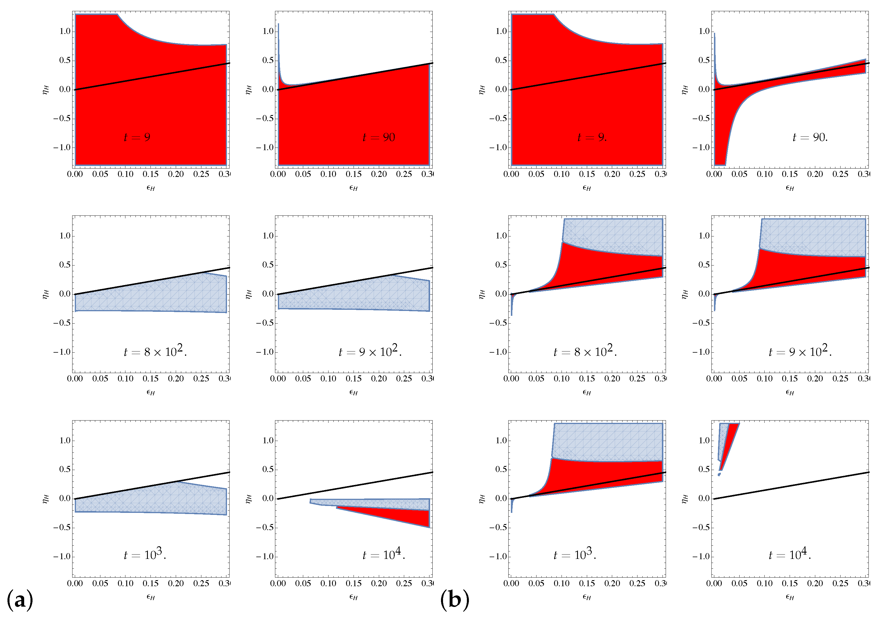
With the purpose to verify whether inequalities (9) and (27) (which we rewrite here for accessibility)

$$\begin{array}{cc}\hfill \dot{S}({ϵ}_H,{\eta }_H)& \le \frac{2\pi }{H}{ϵ}_H\hfill \\ \hfill \ddot{S}({ϵ}_H,{\eta }_H)& \le 4\pi {ϵ}_H(\frac{3}{2}{ϵ}_H-{\eta }_H),\hfill \end{array}$$

hold for positives10$\dot{S}$ and $\ddot{S}$, we present in Figure 2 the contour plots for selected times for which (9) and (27) are satisfied11. The red contours represent the regions where $\dot{S}<0$ whereas the blue ones are those for which $\dot{S}>0$.

As it is observed, there are conditions in time for which the inequalities are satisfied, but since our expressions for $\dot{S}$ and $\ddot{S}$ implicitly depend on ${\eta }_H$ and ${ϵ}_H$, we find that not always it is possible to find conditions for which $ϵ\ll 1$ and ${\eta }_H<0$. Specifically, we observe that,

• For ${\Omega }^2<0$, at late times, it is possible to fulfill the dSC with the constant $c^{\prime }$ of order 0.5 or less. This implies that, at least for this simple model, there is a contribution to the effective four-dimensional entropy from time-dependent fluxes which allows the dSC to be satisfied. For this to happen, the size of the AH radius must be larger than each of the torus radius. For initial times all the inequalities are satisfied only if $\dot{S}<0$. As time evolves the regions where all the inequalities are satisfied are reduced in size. It is interesting to note that for $t\gg 1$ the regions where all inequalities are satisfied exclude small values of ${\eta }_H$ for $ϵ<0.3$. In summary, this model is consistent with the RdS conjecture only for late times;
• For ${\Omega }^2>0$ we also find that at late times there are conditions for the inequalities to be fulfilled but with positive values for ${\eta }_H$ which are not in agreement with the dSC. However, this case implies that the radius of the AH is smaller than the internal torus. It is possible that this is not an available condition during inflation.

4. Conclusions and Final Comments

We have proposed a relation between the de Sitter conjecture (dSC) with the time dependence of fluxes through the covariant entropy bound (CEB). As an alternative of considering the appearance of towers of massless modes via the distance conjecture, we have focused on the possibility that a string time-dependent flux compactification contributes to entropy, such that the CEB also leads us to a bound on the slow-roll parameters of an expanding four-dimensional Universe.

For that we have assumed that ${ϵ}_H\ll 1$ and that −as a result of the CEB− the time variation of entropy is positive and precisely bounded by it (9). Under these assumptions, we look for conditions on which the entropy profile (as a function on time) determines a bound on the second slow-roll parameter ${\eta }_H$. We have performed this analysis in a single and multi-field inflationary scenarios. For the latter we have reproduced the result by Achúcarro and Palma in [28] by which it is possible to fulfill the first inequality of the dSC while allowing the small-roll parameter ${ϵ}_V$ to be of order one in Planck units. We also have constructed a bound for ${\eta }_V$ in terms of the second time derivative of entropy (27), and studied the implications on the Lyth’s bound were we have observed that in general the bound becomes stronger. It is important to notice that for a null variation on the entropy from extra dimensions, the bounds on ${ϵ}_V$ and ${\eta }_V$ allow them to have values much less than one. Whether the dSC can be fulfilled by non-zero contributions of $\dot{S}$ and $\ddot{S}$ or not, will be determined by a specific model.

Finally, in order to have a concrete example, we have presented a simple toy model where we have computed the contribution to entropy from a time dependent flux compactification on a six-dimensional isotropic torus. By treating fluxes as quantum fields, we have computed the transition amplitude of a given flux configuration fulfilling all constraints as the Tadpole cancellation condition, Bianchi identities, and Dirac quantization. As a result, there is an entropy contribution as a function of time. In this case, entropy S and its derivatives with respect to time, depend on H, ${ϵ}_H$ and ${\eta }_H$. We have plotted values for the slow-roll parameters for different values of time in order to test whether the dSC conjecture is fulfilled, meaning that if ${ϵ}_H\ll 1$ then ${\eta }_H<0$.

We have found that for the case in which the internal toroidal volume is smaller than $R_{AH}^6$, where $R_{AH}$ is the size of the apparent horizon during inflation, there are conditions to satisfy the dSC. Further study is required to consider more realistic scenarios in which a time dependence of fluxes can be considered.

References

1. Vafa, C. The String Landscape and the Swampland 2005. Available online: http://xxx.lanl.gov/abs/hep-th/0509212 (accessed on 30 October 2021).
2. Ooguri, H.; Vafa, C. On the Geometry of the String Landscape and the Swampland. Nucl. Phys. B 2007, 766, 21–33. [Google Scholar] [CrossRef] [Green Version]
3. Palti, E. The Swampland: Introduction and Review. Fortsch. Phys. 2019, 67, 1900037. [Google Scholar] [CrossRef] [Green Version]
4. van Beest, M.; Calderón-Infante, J.; Mirfendereski, D.; Valenzuela, I. Lectures on the Swampland Program in String Compactifications. arXiv 2021, arXiv:2102.01111. [Google Scholar]
5. Danielsson, U.H.; Van Riet, T. What if string theory has no de Sitter vacua? Int. J. Mod. Phys. D 2018, 27, 1830007. [Google Scholar] [CrossRef] [Green Version]
6. Obied, G.; Ooguri, H.; Spodyneiko, L.; Vafa, C. De Sitter Space and the Swampland. arXiv 2018, arXiv:1806.08362 [hep-th]. [Google Scholar]
7. Denef, F.; Hebecker, A.; Wrase, T. de Sitter swampland conjecture and the Higgs potential. Phys. Rev. D 2018, 98, 086004. [Google Scholar] [CrossRef] [Green Version]
8. Andriot, D. On the de Sitter swampland criterion. Phys. Lett. B 2018, 785, 570–573. [Google Scholar] [CrossRef]
9. Garg, S.K.; Krishnan, C. Bounds on Slow Roll and the de Sitter Swampland. J. High Energy Phys. 2019, 11, 75. [Google Scholar] [CrossRef] [Green Version]
10. Ooguri, H.; Palti, E.; Shiu, G.; Vafa, C. Distance and de Sitter Conjectures on the Swampland. Phys. Lett. B 2019, 788, 180–184. [Google Scholar] [CrossRef]
11. Andriot, D. New constraints on classical de Sitter: Flirting with the swampland. Fortsch. Phys. 2019, 67, 1800103. [Google Scholar] [CrossRef] [Green Version]
12. Conlon, J.P. The de Sitter swampland conjecture and supersymmetric AdS vacua. Int. J. Mod. Phys. A 2018, 33, 1850178. [Google Scholar] [CrossRef]
13. Dasgupta, K.; Emelin, M.; McDonough, E.; Tatar, R. Quantum Corrections and the de Sitter Swampland Conjecture. J. High Energy Phys. 2019, 1, 145. [Google Scholar] [CrossRef] [Green Version]
14. Andriot, D.; Roupec, C. Further refining the de Sitter swampland conjecture. Fortsch. Phys. 2019, 67, 1800105. [Google Scholar] [CrossRef] [Green Version]
15. Geng, H. Distance Conjecture and De-Sitter Quantum Gravity. Phys. Lett. B 2020, 803, 135327. [Google Scholar] [CrossRef]
16. Atli, U.; Guleryuz, O. A Solution to the de Sitter Swampland Conjecture versus Inflation Tension via Supergravity. JCAP 2021, 04, 27. [Google Scholar] [CrossRef]
17. Dasgupta, K.; Emelin, M.; Faruk, M.M.; Tatar, R. How a four-dimensional de Sitter solution remains outside the swampland. J. High Energy Phys. 2021, 7, 109. [Google Scholar] [CrossRef]
18. Blumenhagen, R.; Brinkmann, M.; Makridou, A. A Note on the dS Swampland Conjecture, Non-BPS Branes and K-Theory. Fortsch. Phys. 2019, 67, 1900068. [Google Scholar] [CrossRef]
19. Damian, C.; Loaiza-Brito, O. Some remarks on the dS conjecture, fluxes and K-theory in IIB toroidal compactifications. arXiv 2019, arXiv:hep-th/1906.08766. [Google Scholar]
20. Andriot, D.; Marconnet, P.; Wrase, T. Intricacies of classical de Sitter string backgrounds. Phys. Lett. B 2021, 812, 136015. [Google Scholar] [CrossRef]
21. Seo, M.S. Thermodynamic interpretation of the de Sitter swampland conjecture. Phys. Lett. B 2019, 797, 134904. [Google Scholar] [CrossRef]
22. Gong, J.O.; Seo, M.S. Instability of de Sitter space under thermal radiation in different vacua. arXiv 2020, arXiv:hep-th/2011.01794. [Google Scholar]
23. Blumenhagen, R.; Kneissl, C.; Makridou, A. De Sitter Quantum Breaking, Swampland Conjectures and Thermal Strings. arXiv 2020, arXiv:hep-th/2011.13956. [Google Scholar]
24. Kobakhidze, A. A brief remark on convexity of effective potentials and de Sitter Swampland conjectures. arXiv 2019, arXiv:physics.gen-ph/1901.08137. [Google Scholar]
25. Wang, Z.; Brandenberger, R.; Heisenberg, L. Eternal Inflation, Entropy Bounds and the Swampland. Eur. Phys. J. C 2020, 80, 864. [Google Scholar] [CrossRef]
26. Brahma, S.; Shandera, S. Stochastic eternal inflation is in the swampland. J. High Energy Phys. 2019, 11, 16. [Google Scholar] [CrossRef] [Green Version]
27. Agrawal, P.; Obied, G.; Steinhardt, P.J.; Vafa, C. On the Cosmological Implications of the String Swampland. Phys. Lett. B 2018, 784, 271–276. [Google Scholar] [CrossRef]
28. Achúcarro, A.; Palma, G.A. The string swampland constraints require multi-field inflation. J. Cosmol. Astropart. Phys. 2019, 2, 41. [Google Scholar] [CrossRef] [Green Version]
29. Heisenberg, L.; Bartelmann, M.; Brandenberger, R.; Refregier, A. Dark Energy in the Swampland. Phys. Rev. D 2018, 98, 123502. [Google Scholar] [CrossRef] [Green Version]
30. Heisenberg, L.; Bartelmann, M.; Brandenberger, R.; Refregier, A. Dark Energy in the Swampland II. Sci. China Phys. Mech. Astron. 2019, 62, 990421. [Google Scholar] [CrossRef]
31. Akrami, Y.; Kallosh, R.; Linde, A.; Vardanyan, V. The Landscape, the Swampland and the Era of Precision Cosmology. Fortsch. Phys. 2019, 67, 1800075. [Google Scholar] [CrossRef]
32. Wang, D. The multi-feature universe: Large parameter space cosmology and the swampland. Phys. Dark Univ. 2020, 28, 100545. [Google Scholar] [CrossRef] [Green Version]
33. Chiang, C.I.; Leedom, J.M.; Murayama, H. What does inflation say about dark energy given the swampland conjectures? Phys. Rev. D 2019, 100, 043505. [Google Scholar] [CrossRef] [Green Version]
34. Matsui, H.; Takahashi, F. Eternal Inflation and Swampland Conjectures. Phys. Rev. D 2019, 99, 023533. [Google Scholar] [CrossRef] [Green Version]
35. Schimmrigk, R. The Swampland Spectrum Conjecture in Inflation. arXiv 2018, arXiv:hep-th/1810.11699. [Google Scholar]
36. Agrawal, P.; Obied, G. Dark Energy and the Refined de Sitter Conjecture. J. High Energy Phys. 2019, 6, 103. [Google Scholar] [CrossRef] [Green Version]
37. Damian, C.; Loaiza-Brito, O. Two-Field Axion Inflation and the Swampland Constraint in the Flux-Scaling Scenario. Fortsch. Phys. 2019, 67, 1800072. [Google Scholar] [CrossRef]
38. Trivedi, O. Implications of single field inflation in general cosmological scenarios on the nature of dark energy given the swampland conjectures. arXiv 2020, arXiv:astro-ph.CO/2011.14316. [Google Scholar]
39. Trivedi, O. Swampland conjectures and single field inflation in modified cosmological scenarios. arXiv 2020, arXiv:2008.05474 [hep-th]. [Google Scholar]
40. Das, S.; Ramos, R.O. Runaway potentials in warm inflation satisfying the swampland conjectures. Phys. Rev. D 2020, 102, 103522. [Google Scholar] [CrossRef]
41. Brandenberger, R.; Kamali, V.; Ramos, R.O. Strengthening the de Sitter swampland conjecture in warm inflation. J. High Energy Phys. 2020, 8, 127. [Google Scholar] [CrossRef]
42. Bousso, R. The Holographic principle. Rev. Mod. Phys. 2002, 74, 825–874. [Google Scholar] [CrossRef] [Green Version]
43. Bousso, R. A covariant entropy conjecture. J. High Energy Phys. 1999, 1999, 4. [Google Scholar] [CrossRef] [Green Version]
44. Bousso, R.; Engelhardt, N. Generalized Second Law for Cosmology. Phys. Rev. D 2016, 93, 024025. [Google Scholar] [CrossRef] [Green Version]
45. Bousso, R.; Casini, H.; Fisher, Z.; Maldacena, J. Proof of a Quantum Bousso Bound. Phys. Rev. D 2014, 90, 044002. [Google Scholar] [CrossRef] [Green Version]
46. Grana, M. Flux compactifications in string theory: A Comprehensive review. Phys. Rept. 2006, 423, 91–158. [Google Scholar] [CrossRef] [Green Version]
47. Blumenhagen, R.; Valenzuela, I.; Wolf, F. The Swampland Conjecture and F-term Axion Monodromy Inflation. J. High Energy Phys. 2017, 2017, 145. [Google Scholar] [CrossRef] [Green Version]
48. Blumenhagen, R.; Damian, C.; Font, A.; Herschmann, D.; Sun, R. The Flux-Scaling Scenario: De Sitter Uplift and Axion Inflation. Fortsch. Phys. 2016, 64, 536–550. [Google Scholar] [CrossRef] [Green Version]
49. Blumenhagen, R.; Font, A.; Fuchs, M.; Herschmann, D.; Plauschinn, E.; Sekiguchi, Y.; Wolf, F. A Flux-Scaling Scenario for High-Scale Moduli Stabilization in String Theory. Nucl. Phys. B 2015, 897, 500–554. [Google Scholar] [CrossRef] [Green Version]
50. Blumenhagen, R.; Herschmann, D.; Plauschinn, E. The Challenge of Realizing F-term Axion Monodromy Inflation in String Theory. J. High Energy Phys. 2015, 1, 7. [Google Scholar] [CrossRef] [Green Version]
51. Cabo Bizet, N.; Damian, C.; Loaiza-Brito, O.; Peña, D.M. Leaving the Swampland: Non-geometric fluxes and the Distance Conjecture. J. High Energy Phys. 2019, 9, 123. [Google Scholar] [CrossRef] [Green Version]
52. Betzler, P.; Plauschinn, E. Type IIB flux vacua and tadpole cancellation. Fortsch. Phys. 2019, 67, 1900065. [Google Scholar] [CrossRef] [Green Version]
53. Sati, H.; Schreiber, U. Equivariant Cohomotopy implies orientifold tadpole cancellation. J. Geom. Phys. 2020, 156, 103775. [Google Scholar] [CrossRef]
54. Cabo Bizet, N.; Damian, C.; Loaiza-Brito, O.; Peña, D.K.M.; Montañez Barrera, J.A. Testing Swampland Conjectures with Machine Learning. Eur. Phys. J. C 2020, 80, 766. [Google Scholar] [CrossRef]
55. Plauschinn, E. Moduli Stabilization with Non-Geometric Fluxes—Comments on Tadpole Contributions and de-Sitter Vacua. Fortsch. Phys. 2021, 69, 2100003. [Google Scholar] [CrossRef]
56. Bena, I.; Blabäck, J.; Graña, M.; Lüst, S. The Tadpole Problem. arXiv 2020, arXiv:hep-th/2010.10519. [Google Scholar]
57. Pinol, L. Multifield inflation beyond Nfield = 2: Non-Gaussianities and single-field effective theory. arXiv 2020, arXiv:astro-ph.CO/2011.05930. [Google Scholar]
58. Chakraborty, D.; Chiovoloni, R.; Loaiza-Brito, O.; Niz, G.; Zavala, I. Fat inflatons, large turns and the η-problem. J. Cosmol. Astropart. Phys. 2020, 1, 20. [Google Scholar] [CrossRef] [Green Version]
59. Lyth, D.H. What would we learn by detecting a gravitational wave signal in the cosmic microwave background anisotropy? Phys. Rev. Lett. 1997, 78, 1861–1863. [Google Scholar] [CrossRef] [Green Version]
60. Scalisi, M.; Valenzuela, I. Swampland distance conjecture, inflation and α-attractors. J. High Energy Phys. 2019, 8, 160. [Google Scholar] [CrossRef] [Green Version]
61. Steinhardt, P.J.; Wesley, D. Dark Energy, Inflation and Extra Dimensions. Phys. Rev. D 2009, 79, 104026. [Google Scholar] [CrossRef] [Green Version]
62. Damian, C.; Loaiza-Brito, O. Meromorphic Flux Compactification. J. High Energy Phys. 2017, 4, 141. [Google Scholar] [CrossRef] [Green Version]
63. Kachru, S.; Schulz, M.B.; Trivedi, S. Moduli stabilization from fluxes in a simple IIB orientifold. J. High Energy Phys. 2003, 10, 7. [Google Scholar] [CrossRef]
64. Akrami, Y.; Arroja, F.; Ashdown, M.; Aumont, J.; Baccigalupi, C.; Ballardini, M.; Banday, A.J.; Barreiro, R.B.; Bartolo, N.; Basak, S.; et al. Planck 2018 results. X. Constraints on inflation. Astron. Astrophys. 2020, 641, A10. [Google Scholar] [CrossRef] [Green Version]
Figure 1. Coordinates of the compact space.
Universe 07 00423 g001
Figure 2. Plots for different times showing the values of η H and ϵ H for which inequalities (9) and (27) are fulfilled with S ¨ > 0 . Red regions are discarded since they are related to a negative value for S ˙ whereas blue regions are related to positive S ˙ . In both cases we take H = 2.5 × 10 3 [64]. (a) Ω 2 < 0 (with Ω 2 = 10 2 ), (b) Ω 2 > 0 (with Ω 2 = 3 × 10 4 ).
Universe 07 00423 g002
Publisher’s Note: MDPI stays neutral with regard to jurisdictional claims in published maps and institutional affiliations.