A Note on the Gravitoelectromagnetic Analogy

Abstract

We discuss the linear gravitoelectromagnetic approach used to solve Einstein’s equations in the weak-field and slow-motion approximation, which is a powerful tool to explain, by analogy with electromagnetism, several gravitational effects in the solar system, where the approximation holds true. In particular, we discuss the analogy, according to which Einstein’s equations can be written as Maxwell-like equations, and focus on the definition of the gravitoelectromagnetic fields in non-stationary conditions. Furthermore, we examine to what extent, starting from a given solution of Einstein’s equations, gravitoelectromagnetic fields can be used to describe the motion of test particles using a Lorentz-like force equation.

1. Introduction

Einstein’s theory of gravitation, General Relativity (GR), completely changed our view and understanding of space and time, as well as the interplay between them. For these reasons, soon after its publication, GR deeply influenced scientific and philosophical thought, even if only few and non-highly accurate observational evidences were available. As emphasised by Will [1], several events, pertaining to both the development of the theoretical framework and observations, contributed to establish the basis of experimental gravitation, starting from the beginning of the 1960s. At first, the great majority of the experimental tests were performed within the solar system; subsequently, observations involving sources outside the solar system were available; in the latter case, we often deal with extreme events producing huge perturbations in the fabric of space–time. On the contrary, in the solar system, the gravitational field is weak but, nonetheless, GR successfully predicts the existence of new phenomena, for which Newtonian gravity is inadequate.

Einstein’s equations in the solar system can be adequately solved in weak-field approximation (small masses, low velocities); in particular, these equations can be written in analogy with Maxwell’s equations for the electromagnetic fields, where the mass density and current play the role of charge density and current, respectively [2,3]. As a consequence, a gravitomagnetic field arises, due to mass currents; more generally, every theory that combines Newtonian gravity with Lorentz invariance predicts the existence of these gravitomagnetic effects. Interestingly enough, the existence of a magnetic-like part of the gravitational field was already suggested by Heaviside, at the end of 1800, on the basis of the similarity between Newton’s law of gravitation and Coulomb’s law of electrostatic force (see McDonald [4] and references therein). This analogy can be exploited to explain GR effects, in terms of electromagnetic ones; this is the case, for instance, of the famous Lense–Thirring gyroscope precession [5], which can be explained in analogy with the precession of a magnetic dipole in a magnetic field.

However, we must always remember that GR is a non-linear theory, so the use of the linear gravitoelectromagnetic (GEM) analogy has some limitations, which need to be emphasised. To this end, it is useful to remember that it is also possible to develop an exact gravitoelectromagnetic analogy in full GR (see, e.g., Cattaneo [6], Costa and Herdeiro [7], Mashhoon et al. [8], Ramos and Mashhoon [9], Costa and Natario [10], Chicone and Mashhoon [11], Rizzi and Ruggiero [12], Jantzen et al. [13], Lynden-Bell and Nouri-Zonoz [14] and also the recent publication by Costa and Natário [15]). The purpose of this paper is to discuss, in full detail, the linear GEM analogy and its limitations. In particular, in Section 2, we discuss, in some detail, the customary approach which, starting from Einstein’s equations in weak-field and slow-motion approximation, leads to the definition of the gravitoelectromagnetic fields. In Section 3, we consider the geodesic equation for a given solution of Einstein’s equations and discuss under which hypotheses it can be formally expressed, in terms of a Lorentz-like force equation for test masses; then, we focus on an application of this formalism to the spacetime of a plane gravitational wave. Discussion and conclusions are given, eventually, in Section 4.

2. Linear Gravitoelectromagnetic Form of Einstein Equations

Let us start from Einstein’s equations:

$$G_{\mu \nu }=\frac{8\pi G}{c^4}{T}_{\mu \nu }.$$

(1)

In the weak-field approximation, the gravitational field can be considered a perturbation of flat spacetime, described by the Minkowski tensor ${\eta }_{\mu \nu }$. 1 As a consequence, the metric tensor can be written in the form $g_{\mu \nu }={\eta }_{\mu \nu }+h_{\mu \nu }$, where $h_{\mu \nu }$ is a weak perturbation: $|h_{\mu \nu }|\ll 1$. If we introduce ${\overline{h}}_{\mu \nu }=h_{\mu \nu }-\frac{1}{2}{\eta }_{\mu \nu }h$, where $h=h_{\mu }^{\mu }$, Einstein’s Equations (1) become (see, e.g., Straumann [16]):

$$-\square {\overline{h}}_{\mu \nu }-{\eta }_{\mu \nu }{\overline{h}}_{\alpha \beta }^{,\alpha \beta }+{\overline{h}}_{\mu \alpha ,\nu }^{\alpha }+{\overline{h}}_{\nu \alpha ,\mu }^{\alpha }=\frac{16\pi G}{c^4}{T}_{\mu \nu }.$$

(2)

The gauge freedom can be exploited setting the Hilbert gauge condition:

$${\overline{h}}_{,\nu }^{\mu \nu }=0.$$

(3)

The above condition is also known as the Einstein, de Donder, Fock, or Lorentz gauge [17]; in particular, the latter name refers to the analogy with the correspondent condition used in electromagnetism (see below). Then, from (2), we get:

$$\square {\overline{h}}_{\mu \nu }=-\frac{16\pi G}{c^4}{T}_{\mu \nu },$$

(4)

Notice that the condition (3) can be always achieved by a gauge transformation; in fact, Einstein’s equations are invariant, with respect to the infinitesimal transformations:

$$h_{\mu \nu }\to h_{\mu \nu }+{\xi }_{\mu ,\nu }+{\xi }_{\nu ,\mu }$$

(5)

which, in terms of ${\overline{h}}_{\mu \nu }$, becomes:

$${\overline{h}}_{\mu \nu }\to {\overline{h}}_{\mu \nu }+{\xi }_{\mu ,\nu }+{\xi }_{\nu ,\mu }-{\eta }_{\mu \nu }{\xi }_{,\alpha }^{\alpha }$$

(6)

So, if ${\overline{h}}_{,\nu }^{\mu \nu }\ne 0$, it is sufficient to choose ${\xi }^{\mu }$ to be a solution of $\square {\xi }^{\mu }=-{\overline{h}}_{,\nu }^{\mu \nu }$.

Equation (4) is in clear analogy with Maxwell’s equations for the electromagnetic four-potential; so, they can be solved in the same way (see, e.g., Ruggiero and Tartaglia [2], Mashhoon [3], Mashhoon et al. [18], Mashhoon [19], and Padmanabhan [20]). In fact, neglecting the solution of the homogeneous wave equations associated with (4), the general solution is given, in terms of retarded potentials:

$${\overline{h}}_{\mu \nu }=\frac{4G}{c^4}{\int }_V\frac{T_{\mu \nu }(ct-|\mathbf{x}-{\mathbf{x}}^{\prime }|,{\mathbf{x}}^{\prime })}{|\mathbf{x}-{\mathbf{x}}^{\prime }|}{\mathrm{d}}^3{x}^{\prime },$$

(7)

where integration is extended to the volume V, containing the source. We may set $T^{00}={\rho }_{}{c}^2$ and $T^{0i}=c{j}_{}^i$, in terms of the mass density ${\rho }_{}$ and current $j_{}^i$ of the source, so that $j_{}^{\mu }=\left(c{\rho }_{},j_g^i\right)=\left(c{\rho }_{},{\mathbf{j}}_{}\right)$ is the mass-current four vector of the source. Since, in linear approximation, ${\displaystyle T_{,\nu }^{\mu \nu }=0}$, we obtain the continuity equation:

$$\frac{\partial \rho }{\partial t}+\nabla ·\mathbf{j}=0$$

(8)

If we assume that the source consists of a finite distribution of slowly moving matter, with $\left|\mathbf{v}\right|\ll c$, then $T_{ij}\simeq \rho v_i{v}_j+p{\delta }_{ij}$, where p is the pressure; from (7), we see that ${\overline{h}}_{ij}=O\left(c^{-4}\right)$, and in the linear GEM approach, we neglect in the metric tensor terms that are $O\left(c^{-4}\right)$.

Consequently, from (7), we get:

$${\overline{h}}_{00}=\frac{4G}{c^2}{\int }_V\frac{\rho (ct-|\mathbf{x}-{\mathbf{x}}^{\prime }|,{\mathbf{x}}^{\prime })}{|\mathbf{x}-{\mathbf{x}}^{\prime }|}{\mathrm{d}}^3{x}^{\prime },$$

(9)

$${\overline{h}}_{0i}=-\frac{4G}{c^3}{\int }_V\frac{j^i(ct-|\mathbf{x}-{\mathbf{x}}^{\prime }|,{\mathbf{x}}^{\prime })}{|\mathbf{x}-{\mathbf{x}}^{\prime }|}{\mathrm{d}}^3{x}^{\prime }.$$

(10)

The other components of ${\overline{h}}_{\mu \nu }$ are zero at the given approximation level.

In analogy with the corresponding solutions of electromagnetism, it is possible to introduce the gravitoelectromagnetic potentials, namely the gravitoelectric ${\Phi }_{}$ and gravitomagnetic $A_{}^i$ potentials are defined by:

$${\overline{h}}_{00}\doteq 4\frac{{\Phi }_{}}{c^2},{\overline{h}}_{0i}=-2\frac{A_i}{c^2},$$

(11)

which, taking into account Equations (9) and (10), take the form:

$$\Phi =G{\int }_V\frac{\rho (ct-|\mathbf{x}-{\mathbf{x}}^{\prime }|,{\mathbf{x}}^{\prime })}{|\mathbf{x}-{\mathbf{x}}^{\prime }|}{\mathrm{d}}^3{x}^{\prime },$$

(12)

$$A_i=\frac{2G}{c}{\int }_V\frac{j^i(ct-|\mathbf{x}-{\mathbf{x}}^{\prime }|,{\mathbf{x}}^{\prime })}{|\mathbf{x}-{\mathbf{x}}^{\prime }|}{\mathrm{d}}^3{x}^{\prime }.$$

(13)

Eventually, the spacetime metric, describing the solutions of Einstein’s equation in weak-field approximation, is written in the form [2,3]:

$$\mathrm{d}{s}^2=-c^2\left(1-2\frac{\Phi }{c^2}\right)\mathrm{d}{t}^2-\frac{4}{c}{A}_i\mathrm{d}{x}^i\mathrm{d}t+\left(1+2\frac{\Phi }{c^2}\right){\delta }_{ij}\mathrm{d}{x}^i\mathrm{d}{x}^j.$$

(14)

Now that we have defined the gravitoelectromagnetic potentials, it is possible to reconsider the Hilbert gauge condition (3) and express it, in terms of ${\Phi }_{}$ and $A_{}^i$. From (3), we obtain, indeed, two conditions; setting $\mu =0$, we get:

$${\overline{h}}_{,0}^{00}+{\overline{h}}_{,i}^{0i}=0\to \frac{1}{c}\frac{\partial \Phi }{\partial t}+\frac{1}{2}\nabla ·\mathbf{A}=0,$$

(15)

which is the same as the Lorenz gauge condition for electromagnetic fields. If we consider the space part ($\mu =i$) of the gauge condition (3), we obtain:

$${\overline{h}}_{,0}^{i0}+{\overline{h}}_{,j}^{ij}=0\to \frac{2}{c^3}\frac{\partial A^i}{\partial t}+{\overline{h}}_{,j}^{ij}=0.$$

(16)

Indeed, even if the terms ${\overline{h}}_{ij}$ are not displayed in the metric (14) for being $O\left(c^{-4}\right)$, they are not necessarily exactly zero. As a consequence, Equation (16) does not imply a time-independent gravitomagnetic potential $\mathbf{A}$.

The issue of the time-independence of the gravitomagnetic potential has been discussed in several papers in the past, still with no general agreement. For instance, Bakopoulos and Kanti [21] explicitly considered ${\overline{h}}_{ij}=0$; hence, from (16), they deduced ${\displaystyle \frac{\partial \mathbf{A}}{\partial t}=0}$, while Harris [22] maintained that ${\displaystyle \frac{\partial \mathbf{A}}{\partial t}=O\left(c^{-2}\right)}$. Similar conclusions about the time independence of the gravitomagnetic field were obtained by Clark and Tucker [23]. For further insights on this topic, we refer to the papers by Costa and Herdeiro [7] and Pascual-Sanchez [24].

According to the approach used by Mashhoon [3], Mashhoon et al. [18], Mashhoon [19], and Ruggiero and Tartaglia [2], the gravitoelectric $\mathbf{E}$ and gravitomagnetic $\mathbf{B}$ fields are defined by:

$$\mathbf{E}=-\nabla \Phi -\frac{1}{2c}\frac{\partial \mathbf{A}}{\partial t},\mathbf{B}=\nabla \wedge \mathbf{A},$$

(17)

and both fields can be time-dependent. In addition, taking Einstein’s Equation (4) into account, we may write the equations for the gravitoelectromagnetic fields in the form:

$$\begin{array}{ccc}\hfill \nabla ·\mathbf{E}& =& 4\pi G\rho ,\hfill \end{array}$$

(18)

$$\begin{array}{ccc}\hfill \nabla \wedge \mathbf{E}& =& -\frac{1}{c}\frac{\partial }{\partial t}\left(\frac{\mathbf{B}}{2}\right),\hfill \end{array}$$

(19)

$$\begin{array}{ccc}\hfill \nabla ·\left(\frac{\mathbf{B}}{2}\right)& =& 0,\hfill \end{array}$$

(20)

$$\begin{array}{ccc}\hfill \nabla \wedge \left(\frac{\mathbf{B}}{2}\right)& =& \frac{4\pi G}{c}\mathbf{j}+\frac{1}{c}\frac{\partial \mathbf{E}}{\partial t}.\hfill \end{array}$$

(21)

In particular, from Equations (18) and (21) the continuity Equation (8) is obtained. We notice the factor $\frac{1}{2}$ near the gravitomagnetic field $\mathbf{B}$, with respect to the original Maxwell’s equations for the electromagnetic fields. This is due to the tensorial character of the gravitational field in GR (see Mashhoon et al. [18]).

It is interesting to point out that if we apply a different gauge condition we obtain different equations for the gravitoelectric and gravitomagnetic fields, as discussed, for instance, by Costa and Natario [10], Bertschinger [25], Damour et al. [26], Carroll [27].

We want to emphasise here an important point: The definition (17) of the gravitoelectric field does not agree with the corresponding one:

$$\mathbf{E}=-\nabla \Phi -\frac{2}{c}\frac{\partial \mathbf{A}}{\partial t},$$

(22)

which we are going to obtain in Section 3, writing the geodesic equation in weak-field and slow-motion approximation. Actually, if we use the definition (22), the source’s equations for the gravitoelectromagnetic fields are modified. As emphasized by Costa and Natario [10], it is not possible to obtain a one-to-one gravitoelectromagnetic analogy both for the geodesic equation and field equations, since, in any case, non-Maxwellian terms appear. Using the definition (22), a different form of the induction law (19) is obtained, which is the same as the one obtained by Bini et al. [28], starting from the gravitoelectromagnetic force acting on a test particle (see next section).

3. Gravitoelectromagnetic Description of the Motion of Test Masses

Let us suppose that the spacetime metric is written in a quite general form:

$$d{s}^2=g_{00}{c}^{2}d{t}^2+2g_{0i}cdtd{x}^i+g_{ij}d{x}^{i}d{x}^j.$$

(23)

By setting:

$$\frac{\Phi }{c^2}=\frac{g_{00}+1}{2}\frac{\Psi }{c^2}=\frac{g_{ij}-1}{2}\frac{A_i}{c^2}=-\frac{g_{0i}}{2}$$

where $|\frac{\Phi }{c^2}|\ll 1$, $|\frac{\Psi }{c^2}|\ll 1$, $|\frac{A_i}{c^2}|\ll 1$, the above metric can be written in the form:

$$\mathrm{d}{s}^2=-c^2\left(1-2\frac{\Phi }{c^2}\right)\mathrm{d}{t}^2-\frac{4}{c}{A}_i\mathrm{d}{x}^i\mathrm{d}t+\left(1+2\frac{\Psi }{c^2}\right){\delta }_{ij}\mathrm{d}{x}^i\mathrm{d}{x}^j,$$

(24)

We do not require that the starting metric (23) be obtained by solving Einstein’s equations in weak-field approximation. In other words, we assume that a given solution of the field equations can be written in this form, and it represents a small perturbation of flat spacetime. In particular, the gravitoelectromagnetic potentials can be time-dependent. The relation between ${\Phi }_{}$ and $A_{}^i$ and the sources can, of course, be obtained by writing the field Equation (2). For instance, this approach was used by Bini et al. [28]; the authors start from a spacetime, in the form (24), assume that the gravitomagnetic potential describes the field of a source whose angular momentum changes with time, and calculate effective sources for the spacetime metric.

Let us start from the line element (24) and calculate the geodesic equation up to linear order in $\beta =\mathbf{v}/c$. From:

$${\frac{{\mathrm{d}}^{2}x}{\mathrm{d}{\tau }^2}}^{\mu }+{\Gamma }_{\alpha \beta }^{\mu }\frac{\mathrm{d}{x}^{\alpha }}{\mathrm{d}\tau }\frac{\mathrm{d}{x}^{\beta }}{\mathrm{d}\tau }=0,$$

(25)

we obtain for the space components:

$$\frac{\mathrm{d}{v}^i}{\mathrm{d}t}=\frac{\partial \Phi }{\partial x^i}-2{(\mathbf{\beta }\times \mathbf{B})}_i+2\frac{\partial A_i}{c\partial t}-{\beta }^i\frac{\partial \left(2\Psi +\Phi \right)}{c\partial t}$$

(26)

(see, e.g., Costa and Natario [10], as well as Bini et al. [28], where the case $\Phi =\Psi$ is considered). Then, if we define the gravitoelectromagnetic fields as:

$$\mathbf{B}=\nabla \wedge \mathbf{A},\mathbf{E}=-\nabla \Phi -\frac{2}{c}\frac{\partial \mathbf{A}}{\partial t},$$

(27)

and the above Equation (26) becomes:

$$\frac{\mathrm{d}{v}^i}{\mathrm{d}t}=-E^i-2{(\mathbf{\beta }\times \mathbf{B})}_i+\frac{2}{c}\frac{\partial A_i}{\partial t}-{\beta }^i\frac{\partial \left(2\Psi +\Phi \right)}{c\partial t}.$$

(28)

As a consequence, it is not warranted that the geodesic equation takes a Lorentz-like form if the fields are not static, due to the presence of the last term in (28). In order to evaluate its impact, we need to compare it with the gravitomagnetic terms ${\displaystyle 2{(\mathbf{\beta }\times \mathbf{B})}_i}$ and ${\displaystyle \frac{2}{c}\frac{\partial A_i}{\partial t}}$. As discussed, for instance, by Thorne and Hartle [29] and Costa and Natário [15], the gravitomagnetic field can be originated by the translation of a source and its spin. In particular, the order of magnitude of the gravitomagnetic field, due to the translation of a source with mass M moving with speed $v_s$, at distance r, is:

$$\left|B_{\mathrm{trans}}\right|\simeq \frac{M{v}_s}{c{r}^2}.$$

(29)

As for the gravitomagnetic field of a spinning source, with angular momentum $\mathbf{S}$, radius R, and peripheral speed $v_{rot}$, we have:

$$\left|B_{\mathrm{spin}}\right|\simeq \frac{S}{c{r}^3}\simeq \frac{M{v}_{rot}R}{c{r}^3}.$$

(30)

Hence, we see that:

$${\left|\mathbf{\beta }\times \mathbf{B}\right|}_{\mathrm{trans}}\simeq \frac{Mv{v}_s}{c^2{r}^2},{\left|\mathbf{\beta }\times \mathbf{B}\right|}_{\mathrm{spin}}\simeq \frac{Mv{v}_{rot}R}{c^2{r}^3}.$$

(31)

For a source like the Earth, the spin contribution is much lower than the translational one, since, typically, $R\ll r$ and $v_{rot}\ll v_s$. We can do similar estimates for the time variation of the vector potential $\mathbf{A}$, and we obtain:

$${\left|\frac{\partial A_i}{c\partial t}\right|}_{\mathrm{trans}}\simeq \frac{M{v}_s^2}{c^2{r}^2},{\left|\frac{\partial A_i}{c\partial t}\right|}_{\mathrm{spin}}\simeq \frac{M{v}_s{v}_{rot}R}{c^2{r}^3}.$$

(32)

As for the last term in (28), we have:

$$\left|{\beta }^i\frac{\partial \left(2\Psi +\Phi \right)}{c\partial t}\right|\simeq \frac{Mv{v}_s}{c^2{r}^2}.$$

(33)

Accordingly, we see that the latter contribution is of the same order as of the translational contribution in (31). It can be neglected, if we assume that the source is at rest or, keeping the spin contribution, when $r{v}_s\ll v_{rot}R$. In addition, we see that, even for a source at rest, in general, the term ${\displaystyle \frac{2}{c}\frac{\partial A_i}{\partial t}}$ cannot be neglected.

The interaction of test masses with the gravitational field can be studied using a variational principle $\delta \int Ldt=0$, starting from the Lagrangian $L=-mcds/dt$, which, according to the Equation (24), is given by:

$$L=-m{c}^2{\left[1-\frac{v^2}{c^2}-\frac{2}{c^2}\left(1+\frac{v^2}{c^2}\right)\Phi +\frac{4}{c^3}{v}_i{A}^i\right]}^{1/2},$$

(34)

which, up to linear order in $\Phi$ and $\mathbf{A}$, and taking the lowest order terms $\mathbf{v}/c$ multiplying the gravitoelectromagnetic potentials, we obtain:

$$\mathcal{L}=-m{c}^2{\left(1-\frac{v^2}{c^2}\right)}^{1/2}+m\Phi -\frac{2m}{c}{v}_i{A}^i.$$

(35)

The term added to the free-particle Lagrangian, ${\displaystyle m\Phi -\frac{2m}{c}{v}_i{A}^i}$, describes the interaction of the test particle with the field. Again, we see that the gravitomagnetic charge is twice the gravitoelectric one. Furthermore, we see that the canonical momentum $\mathbf{P}=\partial L/\partial \mathbf{v}$ is given by ${\displaystyle \mathbf{P}=m\mathbf{v}-\frac{2m}{c}\mathbf{A}}$.

As we are going to show, the geodesic equation takes the form of a Lorentz-like equation when we use Fermi coordinates. The latter are defined starting from the world-line of an observer, and they allow us to show that what an observer measurement depends both on the background field, where she/he is moving. Fermi coordinates are important in the measurement process because they have a concrete meaning, since they are the coordinates an observer would naturally use to make space and time measurements in the vicinity of her/his world-line. This is particularly relevant when dealing with gravitational waves. They are usually studied in the transverse traceless (TT) gauge coordinates (see Flanagan and Hughes [30]), which do not have a physical meaning. An approach to the study of gravitational waves using Fermi coordinates is discussed in Ruggiero [31]. More in general, Fermi coordinates allow us to define a gravitoelectromagnetic analogy in full GR, on the basis of the properties of the Riemann curvature tensor [3,7,8,9,10,11]. In particular, using Fermi coordinates $(cT,X,Y,Z)$, for geodesic observers. The spacetime metric can be written (see, e.g., Ruggiero and Ortolan [32] and references therein) in the form given by Equation (24), with:

$$\begin{array}{ccc}\hfill \Phi (T,X^i)& =& -\frac{c^2}{2}{R}_{0i0j}\left(T\right)X^i{X}^j,\hfill \end{array}$$

(36)

$$\begin{array}{ccc}\hfill A_i^{}(T,X^i)& =& \frac{c^2}{3}{R}_{0jik}\left(T\right)X^j{X}^k,\hfill \end{array}$$

(37)

$$\begin{array}{ccc}\hfill {\Psi }_{ij}(T,X^i)& =& -\frac{2c^2}{3}{R}_{ikjl}\left(T\right)X^k{X}^l.\hfill \end{array}$$

(38)

Notice that $R_{\alpha \beta \gamma \delta }=R_{\alpha \beta \gamma \delta }\left(T\right)$ is the Riemann curvature tensor, evaluated along the reference geodesic, where $X^i=0$, and it depends on T only, which is the observer’s proper time. Then, keeping only terms to first order in $X^i$, we obtain the following expression for the gravitoelectromagnetic fields:

$$E_i^{}(T,X^i)=c^2{R}_{0i0j}\left(T\right)X^j,$$

(39)

and

$$B_i^{}(T,X^i)=-\frac{c^2}{2}{ϵ}_{ijk}{R}_{0l}^{jk}\left(T\right)X^l.$$

(40)

In this case, the third term in Equation (28) vanishes, as it is second order in $X^i$, and the geodesic equation takes the form:

$$m\frac{\mathrm{d}\mathbf{V}}{\mathrm{d}t}=-m\mathbf{E}-2m\frac{\mathbf{V}}{c}\times \mathbf{B}.$$

(41)

Notice that, in this case, $\mathbf{V}$ is the relative velocity, with respect to a test particle on the reference world-line.

As we discussed in our previous papers, Ruggiero and Ortolan [32] and Ruggiero [31], this approach can be applied to the study of the spacetime around a world-line of an observer in the field of a plane gravitational wave. Fermi coordinates were first applied, by Bini et al. [33], to the study of a plane gravitational wave. In particular, if we consider a plane gravitational wave solution, propagating along the x axis with frequency $\omega$, the line element in TT coordinates is given by:

$$d{s}^2=-c^{2}d{t}^2+d{x}^2+(1-h^{+})d{y}^2+(1+h^{+})d{z}^2-2h_{\times }dydz,$$

(42)

where

$$h^{+}=A^{+}sin\left(\omega t-kx\right),h^{\times }=A^{\times }cos\left(\omega t-kx\right).$$

(43)

In the above formulae $A^{+},A^{\times }$ are the amplitude of the wave in the two polarization states, while k is the wave number. Starting from these definitions, and taking into account the fact that, in weak field approximation (up to linear order in the flat spacetime perturbations $h_{\mu \nu }$), the Riemann tensor is invariant, with respect to coordinate transformations, from the definition of the gravitoelectromagnetic fields (39) and (40), we obtain the following expressions in Fermi coordinates:

$$\begin{array}{ccc}\hfill E_X^{}& =& 0,\hfill \end{array}$$

(44)

$$\begin{array}{ccc}\hfill E_Y^{}& =& -\frac{{\omega }^2}{2}\left[A^{+}sin\left(\omega T\right)Y+A^{\times }cos\left(\omega T\right)Z\right],\hfill \end{array}$$

(45)

$$\begin{array}{ccc}\hfill E_Z^{}& =& -\frac{{\omega }^2}{2}\left[A^{\times }cos\left(\omega T\right)Y-A^{+}sin\left(\omega T\right)Z\right],\hfill \end{array}$$

(46)

$$\begin{array}{ccc}\hfill B_X^{}& =& 0,\hfill \end{array}$$

(47)

$$\begin{array}{ccc}\hfill B_Y^{}& =& -\frac{{\omega }^2}{2}\left[-A^{\times }cos\left(\omega T\right)Y+A^{+}sin\left(\omega T\right)Z\right],\hfill \end{array}$$

(48)

$$\begin{array}{ccc}\hfill B_Z^{}& =& -\frac{{\omega }^2}{2}\left[A^{+}sin\left(\omega T\right)Y+A^{\times }cos\left(\omega T\right)Z\right].\hfill \end{array}$$

(49)

Notice that the above expressions and, in particular, the gravitomagnetic field, are explicitly time-dependent.

Using this formalism, it is possible to describe a new example of the action of the gravitomagnetic field of a wave on a moving test mass, determined by the time-dependent gravitomagnetic field. We suppose that a particle is moving on the $YZ$ plane, and hence, orthogonally to the propagation direction of the wave. Since the gravitomagnetic force is ${\mathbf{F}}^B=-2m\frac{\mathbf{V}}{c}\times \mathbf{B}$, the only component of this force is in the X direction. To fix the ideas, let us suppose that, before the passage of the wave, the particle is moving with constant speed $V_0$, along the trajectory:

$$X\left(T\right)=0,Y\left(T\right)=0,Z\left(T\right)=V_{0}T.$$

(50)

Also, we suppose that $A^{\times }=0$. Notice that we neglect the effects of the gravitoelectric field, which are confined to the $YZ$ plane. As a consequence, the only significant equation of motion turns out to be:

$$\begin{array}{ccc}\hfill \frac{{\mathrm{d}}^{2}X}{\mathrm{d}{T}^2}& =& -\frac{V_0^2}{c}{\omega }^2{A}^{+}\left[sin\left(\omega T\right)T\right],\hfill \end{array}$$

(51)

Taking into account the initial conditions, we obtain the following solution:

$$X\left(T\right)=-\frac{V_0^2}{c}{A}^{+}\left[-sin\left(\omega T\right)T+\frac{2}{\omega }\left(1-cos\left(\omega T\right)\right)\right].$$

(52)

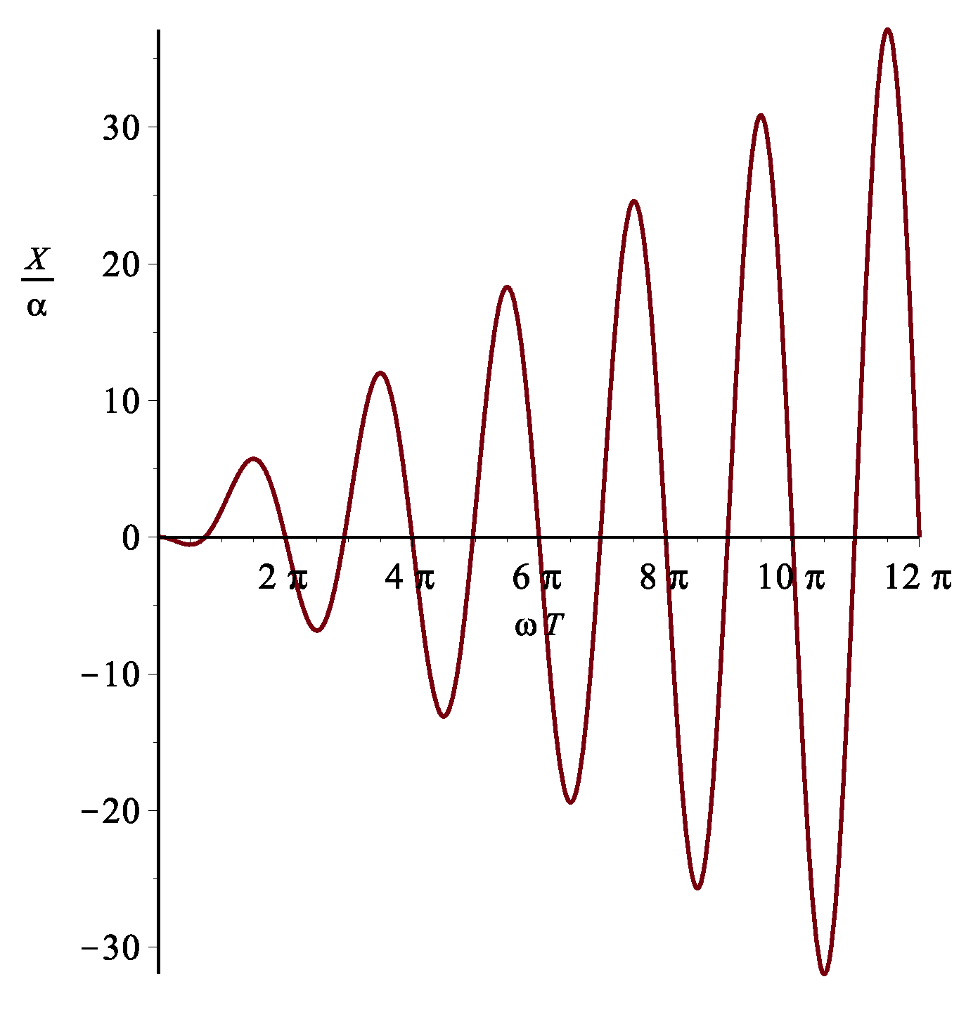
We see that the passage of the wave provokes a motion of the particle out of the $YZ$ plane. The same qualitative result can be obtained for an arbitrary direction of the particle in the $YZ$ plane and considering the other polarization. A sketch of the motion induced by the wave is in Figure 1. The oscillations have increasing amplitude, but they are physically limited, since they are present only during the passage of the wave. It is interesting to point out that the effects that are measured by current intereferometers are on the $YZ$ plane, which is orthogonal to the wave propagation direction, since they are provoked by the gravitoelectric part of the wave field. On the other hand, this is effect (like other ones considered in Ruggiero and Ortolan [32], Ruggiero and Ortolan [34]) is purely gravitomagnetic. As we have seen, it is simply described using this gravitoelectromagnetic approach, but it would be more complicated to understand in the framework of the TT gauge coordinates that are usually employed to describe gravitational waves.

4. Discussion and Conclusions

Many observational tests of general relativity are performed in the so-called weak-field and slow-motion approximation. In other words, the gravitational field can be dealt with as a perturbation of flat spacetime and, moreover, both the sources and test masses have slow speed, compared to the speed of light. In this framework, Einstein’s equations and their solutions can be written in analogy with electromagnetism, and a linear gravitoelectromagnetic formalism can be used. In solving Einstein’s equations, in this approximation, the Hilbert gauge condition is often used. We pointed out that, even if in the solutions for the metric tensor we neglect terms that are $O\left(c^{-4}\right)$, the gravitomagnetic potential and field are not necessarily stationary. Different choices of the gauge conditions lead to a different form for the Maxwell-like equations for the gravitoelectromagnetic fields.

In addition, we considered a general solution of Einstein’s equations that can be written, in terms of a gravitelectric and gravitomagnetic potentials, and used the linear gravitoelectromagnetic analogy to study the motion of test masses. In particular, we discussed under which hypotheses the space components of the geodesic equation have a Lorentz-like form, and showed that this is possible when the sources of the gravitational field are at rest or are very slowly moving. If this is not the case, an extra non Maxwellian-like term is present. This is not surprising. In fact, general relativity and electromagnetism are obviously different theories, and the fact that, in given conditions, there is a similarity, cannot be used to say that gravitation in the weak-field limit is completely analogous to electromagnetism. Moreover, we showed that we recover the Lorentz-like form for the geodesic equation in the framework of Fermi coordinates, to first order in the displacements from the reference world-line. As an application, we used this formalism to study the motion of test masses in the field of a gravitational wave, and showed that, in doing so, purely gravitomagnetic effects arise that are more complicated to understand, in the framework of transverse traceless coordinates, which are often used to study gravitational waves.

We believe that what we have discussed in this note can be useful both to better understand the limitations of the gravitoelectromagnetic analogy and exploit its capability to simplify the description of gravitational phenomena, in its range of applicability.

References

- Will, C.M. Theory and Experiment in Gravitational Physics; Cambridge University Press: Cambridge, UK, 2018. [Google Scholar]
- Ruggiero, M.L.; Tartaglia, A. Gravitomagnetic effects. Nuovo Cim. 2002, B117, 743–768. [Google Scholar]
- Mashhoon, B. Gravitoelectromagnetism: A Brief review. In The Measurement of Gravitomagnetism: A Challenging Enterprise; Iorio, L., Ed.; Nova Science: New York, NY, USA, 2003. [Google Scholar]
- McDonald, K.T. Answer to Question #49. Why c for gravitational waves? Am. J. Phys. 1997, 65, 591–592. [Google Scholar]
- Iorio, L.; Lichtenegger, H.I.M.; Ruggiero, M.L.; Corda, C. Phenomenology of the Lense-Thirring effect in the Solar System. Astrophys. Space Sci. 2011, 331, 351–395. [Google Scholar] [CrossRef] [Green Version]
- Cattaneo, C. General relativity: Relative standard mass, momentum, energy and gravitational field in a general system of reference. Il Nuovo Cimento (1955–1965) 1958, 10, 318–337. [Google Scholar] [CrossRef]
- Costa, L.F.O.; Herdeiro, C.A. Gravitoelectromagnetic analogy based on tidal tensors. Phys. Rev. D 2008, 78, 024021. [Google Scholar] [CrossRef] [Green Version]
- Mashhoon, B.; McClune, J.C.; Quevedo, H. Gravitational superenergy tensor. Phys. Lett. A 1997, 231, 47–51. [Google Scholar] [CrossRef] [Green Version]
- Ramos, J.; Mashhoon, B. Helicity-rotation-gravity coupling for gravitational waves. Phys. Rev. D Part. Fields Gravit. Cosmol. 2006, 73, 084003. [Google Scholar] [CrossRef] [Green Version]
- Costa, L.F.O.; Natario, J. Gravito-electromagnetic analogies. Gen. Rel. Grav. 2014, 46, 1792. [Google Scholar] [CrossRef] [Green Version]
- Chicone, C.; Mashhoon, B. The generalized Jacobi equation. Class. Quantum Gravity 2002, 19, 4231. [Google Scholar] [CrossRef] [Green Version]
- Rizzi, G.; Ruggiero, M.L. The relativistic Sagnac effect: Two derivations. In Relativity in Rotating Frames; Rizzi, G., Ruggiero, M.L., Eds.; Springer: Berlin/Heidelberg, Germany, 2004; pp. 179–220. [Google Scholar]
- Jantzen, R.T.; Carini, P.; Bini, D. The many faces of gravitoelectromagnetism. Ann. Phys. 1992, 215, 1–50. [Google Scholar] [CrossRef] [Green Version]
- Lynden-Bell, D.; Nouri-Zonoz, M. Classical monopoles: Newton, NUT space, gravomagnetic lensing, and atomic spectra. Rev. Mod. Phys. 1998, 70, 427. [Google Scholar] [CrossRef] [Green Version]
- Costa, L.F.O.; Natário, J. Frame-Dragging: Meaning, Myths, and Misconceptions. Universe 2021, 7, 388. [Google Scholar] [CrossRef]
- Straumann, N. General Relativity, With Applications to Astrophysics; Springer: Berlin/Heidelberg, Germany, 2013. [Google Scholar]
- Carroll, S.M. Lecture notes on general relativity. arXiv 1997, arXiv:gr-qc/9712019. [Google Scholar]
- Mashhoon, B.; Gronwald, F.; Lichtenegger, H.I.M. Gravitomagnetism and the Clock Effect. In Gyros, Clocks, Interferometers...: Testing Relativistic Graviy in Space; Springer: Berlin/Heidelberg, Germany, 2001; pp. 83–108. [Google Scholar]
- Mashhoon, B. Gravitational couplings of intrinsic spin. Class. Quantum Gravity 2000, 17, 2399–2409. [Google Scholar] [CrossRef] [Green Version]
- Padmanabhan, T. Gravitation: Foundations and Frontiers; Cambridge University Press: Cambridge, UK, 2010. [Google Scholar]
- Bakopoulos, A.; Kanti, P. From GEM to electromagnetism. Gen. Relativ. Gravit. 2014, 46, 1742. [Google Scholar] [CrossRef] [Green Version]
- Harris, E.G. Analogy between general relativity and electromagnetism for slowly moving particles in weak gravitational fields. Am. J. Phys. 1991, 59, 421–425. [Google Scholar] [CrossRef]
- Clark, S.J.; Tucker, R.W. Gauge symmetry and gravito-electromagnetism. Class. Quantum Gravity 2000, 17, 4125. [Google Scholar] [CrossRef] [Green Version]
- Pascual-Sanchez, J.F. The Harmonic gauge condition in the gravitomagnetic equations. Nuovo Cim. B 2000, 115, 725–732. [Google Scholar]
- Bertschinger, E. Cosmological dynamics: Course 1. In Les Houches Summer School on Cosmology and Large Scale Structure (Session 60); Cornell University: Ithaca, NY, USA, 1993; pp. 273–348. [Google Scholar]
- Damour, T.; Soffel, M.; Xu, C. General-relativistic celestial mechanics. I. Method and definition of reference systems. Phys. Rev. D 1991, 43, 3273. [Google Scholar] [CrossRef]
- Carroll, S.M. Spacetime and Geometry; Cambridge University Press: Cambridge, UK, 2019. [Google Scholar]
- Bini, D.; Cherubini, C.; Chicone, C.; Mashhoon, B. Gravitational induction. Class. Quantum Gravity 2008, 25, 225014. [Google Scholar] [CrossRef]
- Thorne, K.S.; Hartle, J.B. Laws of motion and precession for black holes and other bodies. Phys. Rev. D 1985, 31, 1815. [Google Scholar] [CrossRef] [Green Version]
- Flanagan, E.E.; Hughes, S.A. The basics of gravitational wave theory. New J. Phys. 2005, 7, 204. [Google Scholar] [CrossRef]
- Ruggiero, M.L. Gravitational waves physics using Fermi coordinates: A new teaching perspective. Am. J. Phys. 2021, 89, 639. [Google Scholar] [CrossRef]
- Ruggiero, M.L.; Ortolan, A. Gravito-electromagnetic approach for the space-time of a plane gravitational wave. J. Phys. Commun. 2020, 4, 055013. [Google Scholar] [CrossRef]
- Bini, D.; Geralico, A.; Ortolan, A. Deviation and precession effects in the field of a weak gravitational wave. Phys. Rev. D 2017, 95, 104044. [Google Scholar] [CrossRef] [Green Version]
- Ruggiero, M.L.; Ortolan, A. Gravitomagnetic resonance in the field of a gravitational wave. Phys. Rev. D 2020, 102, 101501. [Google Scholar] [CrossRef]
Figure 1.
The behavior of the particle coordinate parallel to the wave propagation direction; we set .
Publisher’s Note: MDPI stays neutral with regard to jurisdictional claims in published maps and institutional affiliations. |
© 2021 by the author. Licensee MDPI, Basel, Switzerland. This article is an open access article distributed under the terms and conditions of the Creative Commons Attribution (CC BY) license (https://creativecommons.org/licenses/by/4.0/).
Share and Cite
MDPI and ACS Style
Ruggiero, M.L. A Note on the Gravitoelectromagnetic Analogy. Universe 2021, 7, 451. https://0-doi-org.brum.beds.ac.uk/10.3390/universe7110451
AMA Style
Ruggiero ML. A Note on the Gravitoelectromagnetic Analogy. Universe. 2021; 7(11):451. https://0-doi-org.brum.beds.ac.uk/10.3390/universe7110451
Chicago/Turabian StyleRuggiero, Matteo Luca. 2021. "A Note on the Gravitoelectromagnetic Analogy" Universe 7, no. 11: 451. https://0-doi-org.brum.beds.ac.uk/10.3390/universe7110451
Note that from the first issue of 2016, this journal uses article numbers instead of page numbers. See further details here.