
Modeling of Magnetospheres of Terrestrial Exoplanets in the Habitable Zone around G-Type Stars


Skobeltsyn Institute of Nuclear Physics (SINP MSU), Federal State Budget Educational Institution of Higher Education M.V. Lomonosov Moscow State University, 1(2), Leninskie Gory, GSP-1, 119991 Moscow, Russia
*
Author to whom correspondence should be addressed.
Universe 2022, 8(4), 231; https://0-doi-org.brum.beds.ac.uk/10.3390/universe8040231
Submission received: 27 February 2022
/
Revised: 30 March 2022
/
Accepted: 6 April 2022
/
Published: 8 April 2022
(This article belongs to the Special Issue Planetary Plasma Environment)
Abstract
:Using a paraboloid model of an Earth-like exoplanetary magnetospheric magnetic field, developed from a model of the Earth, we investigate the magnetospheric structure of planets located in the habitable zone around G-type stars. Different directions of the stellar wind magnetic field are considered and the corresponding variations in the magnetospheric structure are obtained. It is shown that the exoplanetary environment significantly depends on stellar wind magnetic field orientation and that the parameters of magnetospheric current systems depend on the distance to the stand-off magnetopause point.
1. Introduction
Exoplanetary atmospheres are controlled by the stellar winds and the radiation from their host stars. Stellar winds have existed since the beginning of stellar evolution [1]. The interaction of stellar winds and their magnetic fields with exoplanets is very important for the possibility of life on planets. As a first step in this study, exoplanets from habitable zones (HZ) are considered. In the habitable zone, it is assumed that water can exist on the surface in liquid form. To maintain this condition in particular, a stable atmosphere is needed. The boundaries of the HZ are determined by loss of water and by condensation. We pay attention to the exoplanetary magnetic field, which is very important for the atmosphere and the existence of life. The planetary magnetic field protects the atmosphere from erosion with strong stellar winds. The influence of the stellar wind magnetic field on an exoplanet’s environment was considered, in particular, by Belenkaya et al. [2] and Khodachenko et al. [3].
Stellar winds interacting with exoplanets modify their environment. The cavity around exoplanets, in which the planetary magnetic field prevails over the stellar wind magnetic field and determines plasma behavior, is called the magnetosphere. The boundary of the magnetosphere is the magnetopause. The pressure from stellar wind compresses the magnetopause forward, and an extended magnetotail appears on the opposite side. The interaction of stellar wind with the planetary magnetosphere leads to the formation of magnetospheric current systems, the magnetic field of which contributes to the total magnetospheric field.
Stellar winds have been studied in a series of papers. For example, MacLeod and Oklopčić [4] modeled the interaction between planetary and stellar winds. Cassinelli [5] reviewed theories of stellar winds from luminous stars of early and late types. High-velocity stellar winds from super-giant stars (type O and B) were detected. Vink [6] noted that massive stars are a danger to nearby exoplanets because their stellar winds bring a lot of mass and energy. Johnstone et al. [7] estimate that stellar wind properties for main sequence stars have masses close to that of the sun.
The magnetic field of stellar wind plays a main role in planetary–star interaction (or IMF—interplanetary magnetic field). Unfortunately, at present, our knowledge of magnetized stellar winds is insufficient. Most of this knowledge comes from solar wind study. It is for this reason that research on exoplanets regarding solar-like stars is very active. For example, Reda et al. [8] considered the correlation of solar wind variability with the sun’s activity during five solar cycles. The authors noted that this study is important, not only for the solar system, but also for other solar-type stars in their interactions between the stellar wind and exoplanets. The analogy of stellar wind from sun-type stars with solar wind was used by Nichols and Milan [9] in their study of auroral radio emission due to the stellar wind–exoplanet’s magnetosphere interaction. In the work [10], using 3D MHD models, the authors calculated the Earth’s magnetospheric stand-off distance during the sun’s evolution along the main sequence, dependent on the decreasing solar rotation speed. G-class stars of the Hertzprung–Russell diagram, to which the sun belongs, are yellow with surface temperatures of 5 × 10³–6 × 10³ K. They are X-ray sources. Their spectra contain characteristic lines of iron, sodium, calcium, magnesium, and titanium. Their masses in solar masses are from 0.8 to 1.04, and their sizes are from 0.96 to 1.15 sun radii. The main term in the stellar wind pressure for G stars is the ram pressure, while for M stars it is the magnetic pressure [11,12]. Magnetic field perturbations in stellar wind affect planetary aurora, atmospheres, radio emission, reconstruct the magnetosphere, and can modify the HZ [13,14,15,16,17,18,19,20].
The aim of the paper is to develop the paraboloid model of the terrestrial-like planetary magnetosphere in the habitable zone around a sun-type star. The influence of the stellar wind magnetic field on exoplanetary magnetospheres is of decisive importance. Using a paraboloid magnetospheric exoplanetary model, we show how this effect is realized. Section 2 describes the paraboloid model of the exoplanet’s magnetospheric magnetic field. Numerical results are presented in Section 3. Section 4 contains conclusions.
2. Model Description
The paraboloid magnetospheric magnetic field model was developed based on the terrestrial model by Alexeev [21]. This model includes its own planetary magnetic field, the fields of magnetospheric current systems: the magnetotail and the magnetopause. The partially penetrated magnetic field from the stellar wind is also considered. The coefficient of IMF penetration into the magnetosphere, k, is not known. It may be taken ~0.2, as it is on Earth (for a detailed discussion of this issue, see [22]). The IMF value was arbitrarily chosen to be 100 nT.
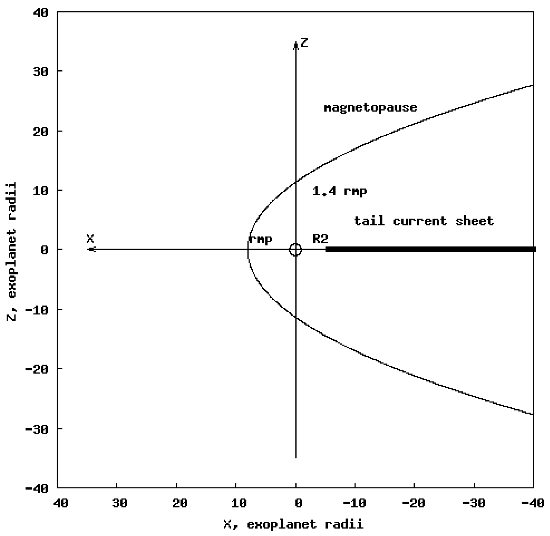
In the model, the shape of the magnetopause is a paraboloid of revolution:
x/rmp = 1 − (y2 + z2)/2rmp2.
The calculations are carried out in the stellar-magnetospheric coordinate system, where the X axis is directed from the planet’s center to the star; the Z axis is perpendicular to X in the plane containing the X and the planetary dipole axes; Y points to dusk perpendicular to X and Z. Here, we ignore the tilt angle between Z and the magnetic dipole axis; rmp is the planetocentric distance to the nose of the magnetopause. In the terminator plane a magnetopause cross-section radius is equal to (2)1/2 rmp or at x = 0 and y = 0, z = 1.4 rmp (see Figure 1).
The axisymmetric shape of the magnetopause is probably due to the symmetry of the supersonic flow around a blunt obstacle (the magnetosphere). Since we do not know the conditions on the fictitious exoplanet, only a very rough model can be used. For this reason, we did not take into account the possible asymmetry of the magnetopause shape associated with the magnetospheric magnetic field asymmetry and assumed an axisymmetric shape for the magnetopause. Experimental data confirm this assumption for Earth [23], Jupiter [24], and Mercury [25].
The planetary magnetic field is a dipole with a value B0 ~3.1 × 10⁴ nT at the equator (as on Earth). The magnetopause current shields all magnetospheric magnetic field sources. The protection of an exoplanet works better if the magnetospheric scale (which is the stand-off distance at the magnetopause, rmp) is much larger than the exobase height [3].
The magnetotail current system consists of cross currents in the equatorial neutral sheet and closure currents at the magnetopause. The distance from the planetary center to the inner edge of the magnetotail current sheet is R2. The magnetic field of the tail current system there is characterized by the parameter Bt. This parameter linearly depends on the flux in the tail lobe Flobe = Btπrmp2/2 [26].
A detailed description of magnetospheric current systems calculated in the paraboloid magnetic field model is given, for example, in Belenkaya et al. [27] for Jupiter and Alexeev et al. [28] for Mercury. The main model parameters used here are: (1) the magnetopause stand-off distance from the exoplanet center, rmp; (2) distance from the exoplanet center to the inner edge of the tail current sheet, R2; (3) magnetic field of the tail current system at the inner edge of the tail current sheet, Bt; (4) components of the stellar wind magnetic field vector (IMF) in the stellar-magnetospheric coordinate system; (5) coefficient of IMF penetration into the magnetosphere, k, chosen equal to 0.2; (6) the magnetic field at the exoplanet equator, B0 and (7) the radius of the exoplanet, Rpl.
The total dipole field plus magnetopause screened current field is considered as curl-free inside the magnetosphere (between the exoplanet and the magnetopause). The scalar potential of the magnetic field of the magnetopause current in the parabolic coordinates was calculated using Bessel functions of the first kind and modified Bessel functions with a singularity at the origin. This is the solution of the Laplace equation for the Neumann problem using integral representations.
The magnetic field of the tail current system is considered as a combination of two parts: the field from the cross-tail current in the infinitely thin current sheet and the field from the closure currents at the magnetopause. For calculations in parabolic coordinates, the magnetic field components were expanded into a mathematical series using Bessel functions of the first kind, modified Bessel functions with singularity at the origin, and the modified Bessel functions without singularity in the magnetosphere.
3. Numerical Results
The equation for rmp for solar type stars can be obtained from the equality of the ram stellar wind pressure Psw and the magnetospheric magnetic field pressure Bm2/2μ0, if we assume that, as for the Earth, the plasma pressure in the exoplanet’s magnetosphere is low.
Psw = Bm2/2μ0
Here, μ0 is the magnetic permeability of the vacuum.
See et al. [20] considered the non-spherical shape of the magnetopause by introducing the coefficient f0~1.16 in the right side of Equation (1). Here, we neglect it, because the value of the planetary dipole is known with a large degree of uncertainty, and this would be an overshoot. For this reason, in the rough estimation, we also do not take into account the Chapmen–Ferroro currents, which increase the magnetospheric magnetic field at the stand-off magnetopause point by 2.4 times. Thus, at the stand-off point Bm = B0Rpl3/rmp3, where B0 is magnetic field at the planet’s equator and Rpl is the exoplanet’s radius.
where Mpl is the exoplanet’s magnetic moment.
Psw = (B0Rpl3/rmp3)2/2μ0.
2μ0Psw = (B0Rpl3/rmp3)2 or 2μ0Pswrmp6 = B02Rpl6 = Mpl2
rmp = [B02Rpl6/(2μ0Psw)]1/6.
See et al. [20] studied 124 sun-like stars with exoplanets in the HZ zone. Their masses were from 0.8 to 1.4 solar masses. The authors suggested that around them in the HZ there are fictitious exoplanets with the same masses, sizes, and magnetic fields as those of the Earth. They determined the ram stellar wind pressure, which allows the formation of magnetospheres comparable in size to the Earth’s. The Parker [29] and Cranmer and Saar [30] models for the stellar wind and star’s mass loss rate, respectively, were used. See et al. [20] calculated the distance from the planet’s center to the front point of the magnetopause rmp. For the selected 10 stars, they determined that rmp for fictitious Earth-type exoplanets were from 8 to 16 RE, where RE is the Earth’s radius RE = 6400 km. Following See et al. [20] we take the magnetic dipole field of a fictitious terrestrial exoplanet equal to the Earth’s with a magnetic moment ME = 3.1 × 10⁴ nT·RE3. Here, we determine the paraboloid magnetospheric magnetic field model parameters for both values of rmp (8 and 16 Rpl).
Following See et al. [20], we consider the minimum and maximum values of rmp for 10 selected fictitious planets around solar-like stars and determine the corresponding Psw from Equation (2). We can determine the magnetic field in the tail lobes Blobe from the equality of Psw-th to the Blobe2/2μ0, where Psw-th is the thermal stellar wind pressure. Since we do not know exactly the stellar wind parameters, we replace Psw-th here by Psw, which is indeed much larger than Psw-th. This will lead to a compression of the tail diameter, which, in some sense, compensates for its anomalous increase in the paraboloid model. The magnetic flux in the tail lobe equals to Flobe = BlobeSlobe, where Slobe = (π/2)Rlobe2. We suppose that Rlobe = 1.4 rmp; Rlobe2 = (1.4)2 rmp2 = 1.96 rmp2 ~2 rmp2.
Flobe = BlobeSlobe = Blobe(π/2) Rlobe2 = πBlobe rmp2
Psw = Blobe2/2μ0.
Blobe2 = 2μ0 Psw.
Flobe = π (2μ0 Psw)1/2 rmp2
The parameter Bt determines the magnetic field at the inner edge of the magnetotail current sheet located at a distance from the planet’s center R2. We assume that
as on Earth. From Johnson et al. [26], for a tail current with zero thickness in the paraboloid model, we obtain:
R2 = 0.7 rmp,
Flobe = 0.5Btπrmp2
Bt = 2Flobe/(πrmp2)
Using Equation (4) we receive:
Bt = 2Flobe/(πrmp2) = 2π(2μ0Psw)1/2 rmp2/(πrmp2) = 2((B0Rpl3/rmp3)2)1/2 = 2B0Rpl3/rmp3
Bt = 2B0Rpl3/rmp3
From Equations (7) and (9) we receive from the selected values of rmp:
- (a)
- rmp = 8RER2 = 0.7 rmp = 5.6 RplBt = 2B0Rpl3/rmp3 = 2B0/83 = 2 × 3.1 × 104 nT/83 = 6.2 × 10⁴ nT/512 = 620 × 102 nT/512 = 121 nT
- (b)
- rmp = 16 RER2 = 0.7 rmp = 11.2 RplBt = 2B0Rpl3/rmp3 = 620 × 102 nT/163 = 620 × 102 nT/4096 = 15 nT.
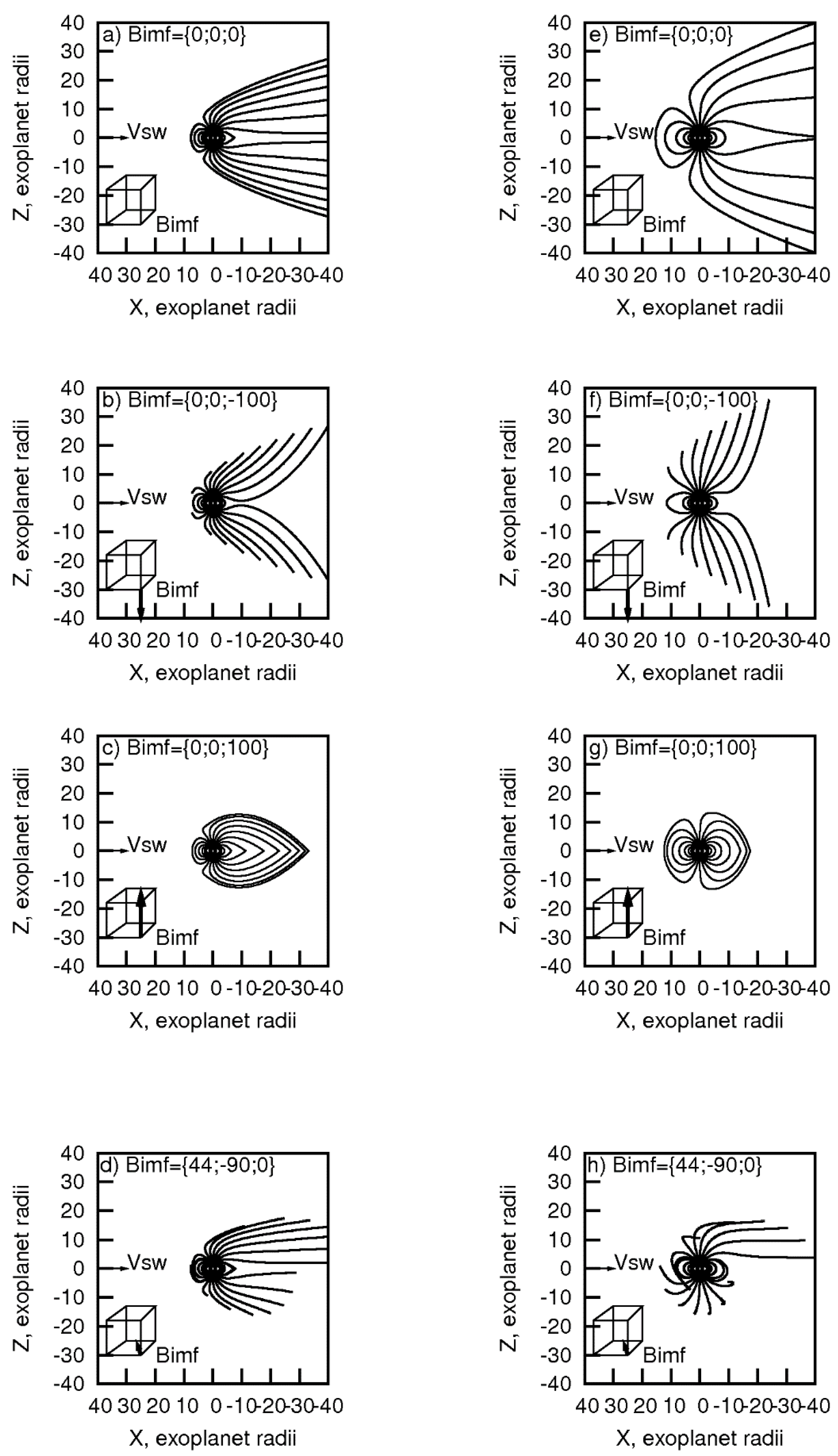
Thus, the stand-off distance rmp is determined by the stellar wind dynamic pressure and the magnetospheric magnetic field, the main input to which gives the planetary dipole in the case of an Earth-like exoplanet around a G-type star. Parameter R2 is taken to be proportional to rmp with a coefficient of ~0.7. Bt depends on the planetary dipole moment Mpl = B0Rpl3 and rmp. Following See et al. [20], we took the rmp values, which they found; the other parameters turned out to be determined by the above equations. Figure 2 presents the results of the calculations.
Figure 2 shows how IMF modifies the magnetospheric magnetic field structure, and how it changes dependent on the rmp value. The structure of the magnetic field when changing the distance to the front point of the magnetopause, rmp, does not change in a similar way due to the non-linear dependence of Bt (the magnetic field of the tail current system at the inner edge of the neutral current sheet) on this parameter.
As the magnetosphere is expended (rmp is greater), the value of the parameter Bt, which determines the magnetic field of the tail current system, decreases, and the influence of the tail becomes smaller. For this case, the high IMF strength ~100 nT (relative to Earth’s environment), which controls the magnetospheric structure, becomes more noticeable. Figure 2b,f show that when the stellar wind magnetic field is parallel to the planetary dipole axis, the tail length for small rmp is ~40 Rpl, while for large rmp it is ~25 Rpl. When the IMF is antiparallel to the dipole of an exoplanet (Figure 2c,g), we have a closed magnetosphere without open field lines, which is located for rmp = 8 Rpl from 8 to −34 Rpl, and for rmp = 16 Rpl from 16 to −20 Rpl. When IMF = 0 (Figure 2a,e), we have open field lines that do not intersect the magnetopause but travel to the distant tail. For strong azimuthal and radial IMF, we see in Figure 2d,h significant asymmetry between the northern and southern hemispheres, which increases for the expanded magnetosphere. These results are new, despite the fact that the effects connected with the stand-off distance for Earth have been studied in many papers [31,32,33,34,35].
4. Conclusions
In this paper, we considered Earth-like exoplanets in the HZ around solar-type stars using a paraboloid model of the magnetospheric magnetic field. Two sets of parameters were considered, corresponding to the minimum and maximum values of the magnetopause stand-off distance determined by See et al. [20] for ten selected fictitious terrestrial planets around sun-type stars. We have considered the influence of the stellar wind magnetic field of different orientations on the magnetospheric magnetic field structure. For this, a paraboloid model of the magnetospheric magnetic field was used. It turns out that the magnetospheric structure significantly depends not only on the orientation of the IMF, but also on the stand-off distance rmp, since all the parameters that determine magnetospheric current systems are controlled by it. Particularly sensitive to rmp is the magnetic field of the tail current system at the inner edge of the neutral current sheet, Bt, which is inversely proportional to rmp3.
For zero stellar wind magnetic field, open field lines do not intersect magnetopause but travel to the distant tail. For IMF antiparallel to the exoplanet’s dipole, the closed magnetosphere without open field lines arises. For the considered stellar wind magnetic field strength ~100 nT, the size of such closed magnetosphere is from 8 to −34 Rpl for rmp = 8 Rpl and from 16 to −20 Rpl for rmp = 16 Rpl. For IMF parallel to the exoplanet’s dipole, the tail length for rmp = 8 Rpl is ~40 Rpl, while for rmp = 16 Rpl it is ~25 Rpl. For strong azimuthal and/or radial IMF, the significant asymmetry between the northern and southern hemispheres arises, which increases for the expanded magnetosphere.
A decrease in the Bt value with the growth of rmp leads to significant reconstruction of the magnetospheric magnetic field. Such a situation was not considered in detail for Earth, despite that the variations in rmp are similar according to the work of Pudovkin et al. [36], for example, who stated that the experimental data suggest the change in the Earth’s stand-off distance from 6.6 to 13.7 terrestrial radii.
Moreover, we consider the stellar wind magnetic field with the value of 100 nT, which does not exist on Earth. It is shown that the influence of such a strong stellar wind magnetic field on the magnetospheric structure increases with the growth of rmp.
Author Contributions
Conceptualization, E.S.B. and I.I.A.; methodology, E.S.B., I.I.A., M.S.B.; software, I.I.A., M.S.B.; validation, I.I.A.; formal analysis, E.S.B., I.I.A., M.S.B.; investigation, E.S.B., I.I.A.; writing—original draft preparation, E.S.B.; writing—review and editing, E.S.B., I.I.A.; visualization, M.S.B.; supervision, E.S.B.; project administration, E.S.B.; All authors have read and agreed to the published version of the manuscript.
Funding
This research received no external funding.
Institutional Review Board Statement
Not applicable.
Informed Consent Statement
Not applicable.
Data Availability Statement
Not applicable.
Acknowledgments
Authors acknowledge the support of Ministry of Science and Higher Education of the Russian Federation under the grant 075-15-2020-780 (N13.1902.21.0039).
Conflicts of Interest
The authors declare no conflict of interest.
References
- Wood, B.E. Astrospheres and solar-like stellar winds. Living Rev. Sol. Phys. 2004, 1, 2. [Google Scholar] [CrossRef] [PubMed] [Green Version]
- Belenkaya, E.; Alexeev, I.; Khodachenko, M.; Panchenko, M.; Blokhina, M. Stellar wind magnetic field influence on the exoplanet’s magnetosphere. In Proceedings of the European Planetary Science Congress, Rome, Italy, 19–24 September 2010; EPSC Abstracts. Volume 5, p. EPSC2010-72. [Google Scholar]
- Khodachenko, M.L.; Sasunov, Y.; Arkhypov, O.; Alekseev, I.; Belenkaya, E.; Lammer, H.; Kislyakova, K.; Odert, P.; Leitzinger, M.; GЁudel, M. Stellar CME activity and its possible influence on exoplanets’ environments: Importance of magnetospheric protection. In Nature of Prominences and Their Role in Space Weather Proceedings IAU Symposium No. 300; Schmieder, B., Malherbe, J.-M., Wu, S.T., Eds.; Cambridge University Press: Cambridge, UK, 2013. [Google Scholar] [CrossRef] [Green Version]
- McLeod, M.; Oklopčić, A. Stellar wind confinement of evaporating exoplanet Atmospheres and its signatures in 1083 nm observations. Astrophys. J. 2022, 926, 226. [Google Scholar] [CrossRef]
- Cassinelli, J.P. Stellar winds. Ann. Rev. Astron. Astrophys. 1979, 17, 275–308. [Google Scholar] [CrossRef]
- Vink, J.S. The theory of stellar winds. arXiv 2011, arXiv:1112.0952. [Google Scholar] [CrossRef]
- Johnstone, C.P.; Güdel, M.; Lüftinger, T.; Toth, G.; Brott, I. Stellar winds on the main-sequence I. Wind model. Astron. Astrophys. 2015, 577, A27. [Google Scholar] [CrossRef] [Green Version]
- Reda, R.; Giovannelli, L.; Alberti, T.; Berrilli, F.; Bertello, L.; del Moro, D.; di Mauro, M.P.; Giobbi, P.; Penza, V. The exoplanetary magnetosphere extension in Sun-like stars based on the solar wind—Solar UV relation. arXiv 2022, arXiv:2203.01554. [Google Scholar] [CrossRef]
- Nichols, J.D.; Milan, S.E. Stellar wind–magnetosphere interaction at exoplanets: Computations of auroral radio powers. Mon. Not. R. Astron. Soc. 2016, 461, 2353–2366. [Google Scholar] [CrossRef] [Green Version]
- Carolan, S.; Vidotto, A.A.; Loesch, C.; Coogan, P. The evolution of Earth’s magnetosphere during the solar main sequence. Mon. Not. R. Astron. Soc. 2019, 489, 5784–5801. [Google Scholar] [CrossRef] [Green Version]
- Zarka, P.; Treumann, R.A.; Ryabov, B.P.; Ryabov, V.B. Magnetically-Driven Planetary Radio Emissions and Application to Extrasolar Planets. Astrophys. Space Sci. 2001, 277, 293–300. [Google Scholar] [CrossRef]
- Zarka, P. Plasma interactions of exoplanets with their parent star and associated radio emissions. Planet. Space Sci. 2007, 55, 598–617. [Google Scholar] [CrossRef]
- Cowley, S.W.H. Asymmetry effects associated with the X component of the IMF in a magnetically open magnetosphere. Planet. Space Sci. 1981, 29, 809–818. [Google Scholar] [CrossRef]
- Cowley, S.W.H.; Morelli, J.P.; Lockwood, M. Dependence of convective flows and particle precipitation in the high-latitude dayside ionosphere on the x and y components of the interplanetary magnetic field. J. Geophys. Res. 1991, 96, 5557–5564. [Google Scholar] [CrossRef] [Green Version]
- Liou, K.; Newell, P.T.; Sibeck, D.G.; Meng, C.-I.; Brittnacher, M.; Parks, G. Observation of IMF and seasonal effects in the location of auroral substorm onset. J. Geophys. Res. 2001, 106, 5799–5810. [Google Scholar] [CrossRef] [Green Version]
- Shue, J.-H.; Newell, P.T.; Liou, K.; Meng, C.-I. Influence of interplanetary magnetic field on global auroral patterns. J. Geophys. Res. 2001, 106, 5913–5926. [Google Scholar] [CrossRef] [Green Version]
- Peng, Z.; Wang, C.; Hu, Y.Q.; Kan, J.R.; Yang, Y.F. Simulations of observed auroral brightening caused by solar wind dynamic pressure enhancements under different interplanetary magnetic field conditions. J. Geophys. Res. 2011, 116, A06217. [Google Scholar] [CrossRef] [Green Version]
- Hu, Z.-J.; Yang, H.-G.; Han, D.-S.; Huang, D.-H.; Zhang, B.-C.; Hu, H.-Q.; Liu, R.-Y. Dayside auroral emissions controlled by IMF: A survey for dayside auroral excitation at 557.7 and 630.0 nm in Ny-Ǻlesund, Svalbard. J. Geophys. Res. 2012, 117, A02201. [Google Scholar] [CrossRef] [Green Version]
- Yang, Y.F.; Lu, J.Y.; Wang, J.-S.; Peng, Z.; Zhou, L. Influence of interplanetary magnetic field and solar windon auroral brightness in different regions. J. Geophys. Res. Space Phys. 2013, 118, 209–217. [Google Scholar] [CrossRef]
- See, V.; Jardine, M.; Vidotto, A.A.; Petit, P.; Marsden, S.C.; Jeffers, S.V.; de Nascimento, J.D., Jr. The effects of stellar winds on the magnetospheres and potential habitability of exoplanets. Astron. Astrophys. 2014, 570, A99. [Google Scholar] [CrossRef] [Green Version]
- Alexeev, I.I.; Belenkaya, E.S.; Kalegaev, V.V.; Lyutov, Y.G. Electric fields and field-aligned current generation in the magnetosphere. J. Geophys. Res. 1993, 98, 4041–4051. [Google Scholar] [CrossRef]
- Alexeev, I.I. The penetration of interplanetary magnetic and electric fields into the magnetosphere. J. Geomag. Geoelectr. 1986, 38, 1199–1221. [Google Scholar] [CrossRef] [Green Version]
- Shue, J.-H.; Song, P.; Russell, C.T.; Chao, J.K.; Yang, Y.-H. Toward predicting the position of the magnetopause within geosynchronous orbit. J. Geophys. Res. 2000, 105, 2641–2656. [Google Scholar] [CrossRef]
- Joy, S.P.; Kivelson, M.G.; Walker, R.J.; Khurana, K.K.; Russell, C.T.; Ogino, T. Probabilistic models of the Jovian magnetopause and bow shock locations. J. Geophys. Res. 2002, 107, 1309. [Google Scholar] [CrossRef] [Green Version]
- Winslow, R.; Anderson, B.; Johnson, C.; Slavin, J.A.; Korth, H.; Purucker, M.E.; Baker, D.N.; Solomon, S.C. Mercury’s magnetopause and bow shock from MESSENGER Magnetometer observations. J. Geophys. Res. 2013, 118, 5. [Google Scholar] [CrossRef]
- Johnson, C.L.; Purucker, M.E.; Korth, H.; Anderson, B.J.; Winslow, R.M.; al Asad, M.M.H.; Slavin, J.A.; Alexeev, I.I.; Phillips, R.J.; Zuber, M.T.; et al. MESSENGER observations of Mercury’s magnetic field structure. J. Geophys. Res. 2012, 117, E00L14. [Google Scholar] [CrossRef]
- Belenkaya, E.S.; Bobrovnikov, S.Y.; Alexeev, I.I.; Kalegaev, V.V.; Cowley, S.W.H. A model of Jupiter’s magnetospheric magnetic field with variable magnetopause flaring. Planet. Space Sci. 2005, 53, 863–872. [Google Scholar] [CrossRef]
- Alexeev, I.I.; Belenkaya, E.S.; Slavin, J.A.; Korth, H.; Anderson, B.J.; Baker, D.N.; Boardsen, S.A.; Johnson, C.L.; Purucker, M.E.; Sarantos, M.; et al. Mercury’s magnetospheric magnetic field after the first two MESSENGER flybys. Icarus 2010, 209, 23–29. [Google Scholar] [CrossRef]
- Parker, E.N. Dynamics of the interplanetary gas and magnetic fields. Astrophys. J. 1958, 664–676. [Google Scholar] [CrossRef]
- Cranmer, S.R.; Saar, S.H. Testing a predictive theoretical model for the mass lost rate of cool stars. Astrophys. J. 2011, 741, 54. [Google Scholar] [CrossRef]
- Schield, M.A. Pressure balance between solar wind and magnetosphere. J. Geophys. Res. 1969, 74, 1275–1286. [Google Scholar] [CrossRef]
- Sibeck, D.G.; Lopez, R.E.; Roelof, E.C. Solar wind control of the magnetopause shape, location, and motion. J. Geophys. Res. 1991, 96, 5489–5495. [Google Scholar] [CrossRef]
- Shue, J.-H.; Chen, Y.-S.; Hsieh, W.-C.; Nowada, M.; Lee, B.S.; Song, P.; Russell, C.T.; Angelopoulos, V.; Glassmeier, K.H.; McFadden, J.P.; et al. Uneven compression levels of Earth’s magnetic fields by shocked solar wind. J. Geophys. Res. 2011, 116, A02203. [Google Scholar] [CrossRef] [Green Version]
- Samsonov, A.A.; Gordeev, E.; Tsyganenko, N.A.; Šafránková, J.; Němeček, Z.; Šimůnek, J.; Sibeck, D.G.; Tóth, G.; Merkin, V.G.; Raeder, J. Do we know the actual magnetopause position for typical solar wind conditions? J. Geophys. Res. 2016, 121, 6493–6508. [Google Scholar] [CrossRef] [Green Version]
- Samsonov, A.A.; Bogdanova, Y.V.; Branduardi-Raymont, G.; Sibeck, D.G.; Toth, G. Is the relation between the solarwind dynamic pressure and the magnetopause standoff distance so straightforward? Geophys. Res. Lett. 2020, 47, e2019GL086474. [Google Scholar] [CrossRef]
- Pudovkin, M.I.; Besser, B.P.; Zaitseva, S.A. Magnetopause stand-off distance in dependence on the magnetosheath and solar wind parameters. Ann. Geophys. 1998, 16, 388–396. [Google Scholar] [CrossRef]
Figure 1.
The scheme illustrates used parameters in the paraboloid model.

Figure 2.
The figure shows variations of magnetospheric magnetic field structure for rmp = 8 Rpl, R2 = 5.6 Rpl, Bt = 121 nT (left column; subfigures (a–d)) and rmp = 16 Rpl, R2 = 11.2 Rpl, Bt = 15 nT (right column; subfigures (e–h)) for different orientations of the stellar wind magnetic field (IMF). The components of the IMF are given for each image. The coefficient of IMF penetration k = 0.2. Magnetic field lines projected on the plane XZ are plotted. Vector Vsw marks the average stellar wind velocity.

Publisher’s Note: MDPI stays neutral with regard to jurisdictional claims in published maps and institutional affiliations. |
© 2022 by the authors. Licensee MDPI, Basel, Switzerland. This article is an open access article distributed under the terms and conditions of the Creative Commons Attribution (CC BY) license (https://creativecommons.org/licenses/by/4.0/).
Share and Cite
MDPI and ACS Style
Belenkaya, E.S.; Alexeev, I.I.; Blokhina, M.S. Modeling of Magnetospheres of Terrestrial Exoplanets in the Habitable Zone around G-Type Stars. Universe 2022, 8, 231. https://0-doi-org.brum.beds.ac.uk/10.3390/universe8040231
AMA Style
Belenkaya ES, Alexeev II, Blokhina MS. Modeling of Magnetospheres of Terrestrial Exoplanets in the Habitable Zone around G-Type Stars. Universe. 2022; 8(4):231. https://0-doi-org.brum.beds.ac.uk/10.3390/universe8040231
Chicago/Turabian StyleBelenkaya, Elena S., Igor I. Alexeev, and Marina S. Blokhina. 2022. "Modeling of Magnetospheres of Terrestrial Exoplanets in the Habitable Zone around G-Type Stars" Universe 8, no. 4: 231. https://0-doi-org.brum.beds.ac.uk/10.3390/universe8040231
Note that from the first issue of 2016, this journal uses article numbers instead of page numbers. See further details here.