A Mesofractal Model of Interstellar Cloudiness

Abstract

The interstellar medium (ISM), serving as a background for the propagation of cosmic rays (CRs) and other information carriers, has a complex ragged structure. Being chaotically scattered over interstellar space, together with the magnetic field perturbations frozen in them, CRs are connected with each other by a network of magnetic field lines creating long-range correlations of a power-law type, similar to those observed in the spatial distribution of galaxies. These lines solving interstellar transfer problems require the choice of an ISM model, adequately and concisely representing their statistical properties. This article discusses one such model, the Uchaikin–Zolotarev model: a four-parameter approximation of the power spectrum spatial correlations, derived from the generalized Ornstein–Zernike equation. The numerical analysis confirmed that this approximation satisfactorily agrees with the numerical data obtained in the quasi-linear model of plasma turbulence.

1. Introduction

Starlight, cosmic rays, and other observed messengers bring us information about distant parts of the Universe. Passing through the interstellar galactic medium, the charged component of cosmic rays (CRs) experiences the influence of the interstellar medium (ISM) and loses some information about the sources. In order to restore this, one should take into account the influence of the ISM on the information, carried through it from CR sources. The main property of the ISM is its turbulence thanks to which the initial idea arose about the similarity of the cosmic rays’ motion to Brownian motion and describing it in terms of the ordinary diffusion process. However, Brownian motion takes place in a homogeneous uncorrelated medium, whereas the ISM is not such a medium: the turbulent magnetic fields penetrating it create spatially correlated structures. They are reflected in the framework of the quasi-linear theory, called below the wave model. It takes into account the turbulence influence, assuming that it is uniform, isotropic, and has Kolmogorov’s power spectrum (see, e.g., [1]). The mathematical way of constructing a turbulent medium in the frame of this approach runs through the expansion of the field into the plane waves with random amplitudes and phases and involves the perturbation theory. We call this scheme the wave model. The visual image of such a medium in this case is represented by a set of random magnetic field lines surrounded by spiral trajectories of CR charged particles.

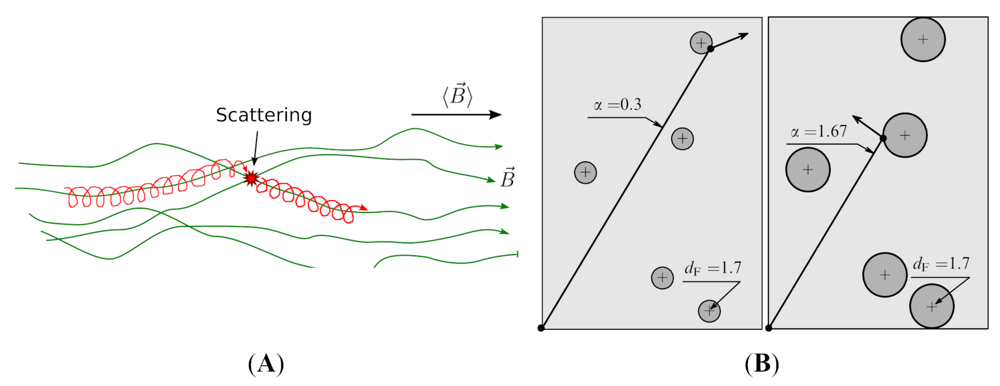
However, astronomical observations reveal some other patterns in the ISM: it has an “island” and cloudy character, and cloud densities, as Fermi noted in [2], can be as much as tens and hundreds of times higher than the average ISM density. At the same time, the magnetic fields “frozen” in CRs, together with gravitational forces create long-range correlations of a power-law type, similar to those observed in the spatial distribution of galaxies. Despite the obvious difference between the visual images of these two models, they have one important property: the similarity of the statistical description at different scales. Astrophysicists F. Combes [3,4], A. Dudorov [5], J. Scalo [6], and A. Baryshev [7,8] paid attention to this similarity, which is determined as fractality or the multiscale hierarchy of the ISM. The visual patterns of both models are sketched in Figure 1.

However, this analysis was accompanied by the use of only one attribute of turbulence in its simplest form $k^n$, known in astrophysics as the Harrison–Zeldovich spectrum.

Our previous studies showed that this may be a rather rough tool, which does not confidently distinguish between samples even within statistically homogeneous groups of galactic surveys in [9]. At the same time, using the four-parameter UZ ansatz has been well proven in the spatial galaxy distribution (SGD) problem. Inspired by this successful application, we decided to implement the comparative statistical analysis of the ISM and SGD by using the four-parameter UZ ansatz. Moreover, the first part of the program (SGD analysis) can be considered as complete, and what remained for us to do was to execute the second part of the program (ISM analysis). This topic is the subject of the present work.

Unlike the wave ISM model based on the system of MHD differential equations including the Navier–Stokes equation, the mesofractal cloud model underlies the generalized Ornstein–Zernike integral equation. Nevertheless, both models reveal a specific property of symmetry, called fractality. Mathematical aspects of this approach were presented in works [10,11]; some modeling algorithms were given in [12,13,14]; the results of its successful application to the statistics of the spatial distribution of galaxies were shown in [15,16]. Based on the Lévy-stable theory, V. Uchaikin and V. Zolotarev suggested a new ansatz for fitting fractal properties of random point systems, occupying an intermediate place between the class of homogeneous media and the class of fractals.

Figure 2, obtained by direct Monte Carlo simulations according to the algorithm, elaborated in [14], demonstrates the main property of the mesofractal: at small scales, it looks the same as a pure fractal (a monofractal with a fractional dimension); at large scales, it appears as a uniform Poisson distribution. Our recent investigations [9], related to the galaxy power spectrum in the Universe, confirmed the robustness and efficiency of the new approximation of random fractal-like structures.

The purpose of this work was to test this approach as applied to the interstellar medium, the properties of which determine the fluxes of cosmic rays and other information carriers in the Galaxy.

2. ISM Turbulence: The Wave Model

The key feature of the ISM is its turbulence. Turbulence means the chaotic motions in a fluid leading to the diffusion of matter and the dissipation of kinetic energy. Because of its chaotic nature, turbulence can only be studied and modeled in terms of statistical quantities. The motion of molecular and dust flows is controlled on average by the Navier–Stokes equations. They introduce non-locality, remaining a characteristic feature of the non-local cosmic ray theory [17].

The important (in the sense of a collective variable approach) concept of the power spectrum was introduced by Kolmogorov in 1941 [18]. This theory assumes the non-linear wave–wave interaction that results in the energy cascade through smaller scales. The presence of charged particles transmutes the ISM into plasmas. Compressible plasmas play a significant role in the formation of a hierarchy of density structures, viewed as dense cores nested in less-dense regions, which are in turn embedded in low-density regions, and so on. Such a hierarchical structure was described by von Weizsäcker in [1] as:

$$\frac{{\rho }_{\nu }}{{\rho }_{\nu -1}}={\left(\frac{l_{\nu }}{l_{\nu -1}}\right)}^{-3\alpha },$$

where ${\rho }_{\nu }$ represents the average density of a structure at hierarchical level $\nu$ at a length scale l and $\alpha$ the compressibility degree, assumed to be the same at each level. The dimensionality of the system is $3-3\alpha$, and the average mass within each substructure must follow the relation $M_l\propto l^{3-3\alpha }$. Currently, such structures are called fractals. One can think that this is the main reason for which the transport equations for cosmic rays in a turbulent ISM are expressed through the fractional operators (for details, see [19]).

The classical way of solving a system of differential equations describing continuum flows’ behavior is based on the representation of their solution in the form of a superposition of plane harmonic waves. The boundary conditions determined by the problem statement form the spectra of wave vectors, thereby discretizing the initially continuous system. Associated with the original coordinate system, the phase space takes the form of cells (lattices, grids), thereby provoking the transition from continuous functions differentiable along the continuum to their discrete approximation and difference schemes for their solutions. See, for instance, [20], where the magnetohydrodynamic (MHD) equations were solved in Cartesian geometry (x-y plane) over a region with dimensions $x_{max}\times y_{max}$. The simulation began with the fluid consisting of a uniform flow in the positive x-direction with a given speed and a turbulent density. The density fluctuations were generated in this calculation by the composition of a few two-dimensional Kolmogorov-like power-law spectra of the form:

$$G\left(k\right)\propto \frac{1}{1+{\left(bk\right)}^{\gamma }},$$

(1)

where k is the magnitude of the wavevector, b is the turbulence coherence length, and $\gamma$ is a spectral index. The turbulence was generated by summing over a large number of discrete wave modes. The authors chose the conditions in such a way that the maximum wavelength was $5b$ and the minimum wavelength was $0.005b$. The grid-cell size was of the smallest wavelength of the system. The coherence scale of the turbulent fluctuations, b, determined the scale of these simulations since MHD has no intrinsic scale.

3. An Alternative Model—The Cloud Model

Traditionally, converting a continuous image of the irregular nonhomogeneous medium, obtained using a telescope or MHD calculation, into a point set more suited for statistical processing is performed by the peak methods, or the density level. The natural localized inhomogeneities of the ISM make the problem easier to solve. The molecular clouds (MCs) are a fundamental ingredient of galaxies: they are the channels that transform the diffuse gas into stars and play an essential role both in the understanding of the dynamic process and its statistical description [21].

The first interpretation of the interstellar medium in terms of a set of localized formations randomly scattered in space was given in the pioneering work of E. Fermi concerning the origin of cosmic rays [2]. He assumed that the interstellar space of the galaxy is occupied by matter at extremely low density, about one atom per ${\mathrm{cm}}^3$, However, it is not uniformly distributed, but there are condensations where the density may be as much as ten- or a hundred-times as large, which extend to average dimensions of the order of 10 pc. Such relatively dense clouds occupy approximately 5% of the interstellar space.

In [22], the ISM was treated as a set of giant molecular clouds (GMCs) scattered in space. On the assumption that they are randomly (i.e., uniformly) distributed in the gas disc, each has a radius $R=20$ pc, and all the clouds combined occupy a fraction $f=3\times {10}^{-3}$ of the gas-disc volume. The article ended with a remark to which the authors draw special attention: “one has to be cautious about using a steady-state approximation and neglecting space fluctuations”. This remark can be considered as a hint about the Poissonian statistics of the medium, because the spatial correlations are neglected. However, astrophysical observations demonstrate not only the crucial role of the correlations, but their long-tail inverse power type.

The cloud-studded structure of the ISM can be considered as an important argument in favor of the model of random distributions of localized objects in comparison with the model of harmonic waves with random amplitudes and phases. It makes the general picture of the system more visual in the physical sense and more operational in the statistical relation.

4. Fractal Dust

Characterizing the position of each object by an isolated point and postulating the self-similarity of their spatial distribution (confirmed by numerous astronomical observations), we arrive at a simple and convenient model, introduced by Benoit Mandelbrot and called by him fractal dust [23]. The prototype of this concept was the spatial distribution of galaxies: observational data showed whichever galaxy we choose as the origin, the number of its neighbors in a ball of radius R grows with the radius increasing as $F{R}^D$, where the exponent $D\in (1,2)$ is called the fractal dimension, and the factor F was initially considered a random variable. In a more rigorous approach, developed by Peebles in [24], this property was formulated as $\langle N\left(R\right)\rangle =A{R}^D$, where $A=\langle F\rangle$ is now a deterministic constant, the value of which depends on the family of galaxies included in the sample.

The Mandelbrot idea, that the observed correlations of the power type can be provided by organizing random walks with rectilinear segments of random length, distributed according to a power law, has been highly fruitful (see [3,8,24,25]), but such a construction violated the symmetry principle: the starting point differed in its environment from other nodes of this trajectory. This question was solved in [12] by constructing a symmetric (in the statistical sense) trajectory starting from the same point and imitating both parts (the past and the future) of a single trajectory. The set of its nodes forms, by Mandelbrot’s definition, a pure fractal, possessing the same statistical property around each point. As for the application to the Universe, Mandelbrot wrote in [26]: “The Universe is a self-similar fractal only up to a crossover scale that satisfies $0<R_{cross}<\infty$, and the crossover between the fractal and the homogeneous ranges occurs very sharply. That is, there is no transient range of significant width, whose structure would require additional parameters in order to be specified”.

The mesofractal model covers both regions: of small scales and of large scales. The first one was considered in the papers [10,11,15]. There, the structure function method was used, allowing the investigation of small-scale turbulence by using the first terms of the Ornstein–Zernike equation solution in the Neumann series, showing quite satisfactory results. Coming to larger scales, we apply an alternative approach—the power spectrum representation, covering in compact form all other terms of the Neumann series. These calculations were specially performed to answer remarks on the quasi-linear turbulence model. As one can see from the two new pictures (Figure 1), the UZ approximation gives very close results to quasi-linear theory [20] as well. Moreover, instead of sharp artificial truncations at inertial domain boundaries, we observe more smooth transitions through the crossovers. These results were included in the new version of the paper.

5. The Mesofractal Model

Such a system was theoretically built and investigated by V. Uchaikin et al. in [10,13,16,27] and called, for short, the mesofractal. This term was offered instead of “fractal with turnover to homogeneity”, mostly for the sake of brevity. A mesofractal differs from a fractal in that as you zoom in, it looks more and more uniform. At the same time, the homogeneity property of the fractal is preserved, which boils down to the fact that this effect is equally manifested in all areas of this mesofractal. Wherever we choose the center of the sphere, the number of points inside it, with increasing radius, first grows according to the fractal law and then according to the law of a homogeneous medium. The construction of such a model is carried out in the following order. First, a homogeneous Poisson distribution is modeled. This set of points is a seed set of initial nodes of independent Markov chains. The first generation is formed by a set of shifts of these points by independent random vectors distributed according to the isotropic Lévy–Feldheim law with a characteristic exponent $\alpha$. The convolutions of these distributions, due to their property, reproduce the distributions of the same family, but with a changed (increased) length scale, which ensures the asymptotical power behavior of the correlation functions. The second-generation of nodes arises from the first in the same way. Of course, if the bare distribution is homogeneous and unlimited, then any generation will be the same, and the average value of the density, together with its highest moments, will turn to infinity. However, if we introduce a small probability of breaking the trajectories at each node, the average number of nodes on the trajectory will become finite, and at the same time, the density of the number of nodes in space will also become finite, while the declared properties of the mesofractal will also appear.

6. The Uchaikin–Zolotarev Power Spectrum and Ornstein–Zernike Equation

The key role in the MC arrangement simulation procedure belongs to the Uchaikin–Zolotarev (UZ) approximation of the power spectrum:

$$P_{UZ}\left(k\right)=A\frac{e^{-{\left(bk\right)}^{\alpha }}}{1-c{e}^{-{\left(bk\right)}^{\alpha }}},$$

(2)

where k is a wave-vector modulus, A is a normalizing constant, b is a length scale, $c\in (0,1]$, and $\alpha \in (0,2]$.

In order to understand what sort of information about the structure can be extracted from Equation (2), we return for a minute to the article [11], where this model was introduced. The function $exp\{-{\left(bk\right)}^{\alpha }\}$ is a characteristic function of the Lévy–Feldheim 3D isotropic stable distribution, describing here random paths between consecutive clouds placed in space. The sequence of them forms a chain — the broken line, the nodes of which indicate the positions of magnetic clouds scattering cosmic rays. Each such chain starts from an initial point, the set of which composes a uniform Poisson ensemble of independent random points. These chains are mutually independent and not infinite: each of them can break at the next node with probability $1-c$. The average concentration of seed nodes is $n_0$ (included in the normalizing parameter A), and the concentration of all nodes (the average number of clouds per unit volume) is $n=n_0/(1-c)$. Note, that b is, in order of magnitude, the distance between successive clouds in the trajectory (not mixing with the nearest neighbors). The details of this theory may be found in [10].

The power spectrum (2) admits a clear interpretation of the procedure described in terms of the Ornstein–Zernike (OZ) equation, applied, however, not to molecules, but to interstellar clouds. Really, the UZ spectrum obeys the equation [10]:

$$P\left(k\right)=A{e}^{-{\left(bk\right)}^{\alpha }}+c{e}^{-{\left(bk\right)}^{\alpha }}P\left(k\right),$$

(3)

in the coordinate space having the form of the two-point correlation function:

$$\xi \left(\mathbf{x}\right)=A{b}^{-3}p(\mathbf{x}/b;\alpha )+c{b}^{-3}\int p(\mathbf{x}/b)\xi (\mathbf{x}-{\mathbf{x}}^{\prime })d{\mathbf{x}}^{\prime },$$

(4)

where $p(\mathbf{x};\alpha )$ is a three-dimensional stable Lévy–Feldheim distribution (with characteristic function $\exp \{-{\left|\mathbf{k}\right|}^{\alpha }\}$) [10].

This is the Fredholm integral equation of the second kind known in statistical hydromechanics as the Ornstein–Zernike (OZ) equation for the pair correlation function describing the correlation properties of a homogeneous isotropic liquid. The OZ equation expresses the idea that the total correlation between particles (in our case, between clumps) arises primarily from the direct correlation effect, but with a correction arising from higher-order effects that bring in more and more additional clumps. This leads to the interpretation of direct correlation as the correlation effect between just two objects in a homogeneous background density.

7. The OZ Equation Interpretation

Following Stell’s paper [28], we recall the main points of derivation (4). Stell considered a simple, homogeneous fluid of some localized objects (in our case, clouds) with a mean number density (concentration) $\rho$. The radial distribution function $g\left(r\right)$ (where $r=\left|{\mathbf{x}}_1-{\mathbf{x}}_2\right|$) expresses the extent to which the density is modified by correlations; so if there is an object at position ${\mathbf{x}}_1$, the density at ${\mathbf{x}}_2$ will be $\rho g\left(\right|{\mathbf{x}}_1-{\mathbf{x}}_2\left|\right)\equiv \rho g_{12}$. At a long range, the correlations die out, so $g\left(r\right)\to 1$ as $r\to \infty$. The shifted quantity $\xi =g-1$ (the total correlation function) and is related to the direct correlation function $c_{12}$ via the OZ equation:

$${\xi }_{12}=c_{12}+\rho \int d{\mathbf{x}}_3{c}_{13}{\xi }_{32}.$$

(5)

It expresses the idea that the total correlation between particles arises primarily from the direct correlation effect, but with a correction arising from higher-order effects that bring in more and more additional particles. This leads to the interpretation of the direct correlation as the correlation effect between just two particles (in our terminology, objects) in a homogeneous background density.

With this in mind, the OZ equation can be “derived” based on the following physical arguments:

• Assume there is an object at position ${\mathbf{x}}_1$;
• The direct correlation effect modifies the density at ${\mathbf{x}}_2$ by an amount $\rho c_{12}$;
• The density at ${\mathbf{x}}_3$ is modified as well, by an amount $\rho c_{13}$;
• This fluctuation at ${\mathbf{x}}_3$ has an additional effect on the density at ${\mathbf{x}}_2$, with magnitude $\rho c_{13}\rho c_{32}$;
• Object 3 can be anywhere, and after integrating over ${\mathbf{x}}_3$ and canceling one power of $\rho$, one obtains:

  $${\xi }_{12}\approx c_{12}+\rho \int d{\mathbf{x}}_3{c}_{13}{c}_{32};$$

  (6)
• The entire argument can be repeated with more intermediate particles, giving the infinite series:

  $${\xi }_{12}=c_{12}+\rho \int d{\mathbf{x}}_3{c}_{13}{c}_{32}+{\rho }^2\int d{\mathbf{x}}_3{c}_{13}\int d{\mathbf{x}}_4{c}_{34}{c}_{42}\cdots ;$$

  (7)
• Finally, this series can be summed by a simple substitution to give the OZ equation.

Matching UZ approximations with known MHD-calculated or experimentally observed data allows finding numerical values of the material parameters listed above. In our previous work [9], we tested this procedure on galactic catalogs and obtained good results. This inspired us to extend this approach to the interstellar analysis.

Let us note that for $c=1$ and small b, the UZ formula becomes the Harrison–Zeldovich (HZ) spectrum:

$$P_{HZ}\left(k\right)={\left(bk\right)}^{-\alpha },\alpha <3,$$

(8)

corresponding to a pure fractal (mono-fractal) structure. Furthermore, when $b\to \infty$, the exponential functions vanish, and we obtain the spectrum corresponding to the homogeneous Poisson distribution. Applying to the right side of the spectrum (2) the formula for the sum of a geometric progression and taking into account that $exp\left\{-n{\left(bk\right)}^{\alpha }\right\}$ are the characteristic functions of isotropic definitions of a fractal type, we see that the mesofractal can be considered as a special case of the multifractal dust with a discrete dimensionality spectrum containing only two values, $D=\alpha$ and $D=3$, and may called for this reason bifractal [29].

8. Mesofractal Modeling

The Monte Carlo simulation of a mesofractal system with given parameters includes the following steps:

• A homogeneous Poisson ensemble of random points is constructed in three-dimensional space;
• Each of them is taken as a seed node for the implementation of a 3D Markov chain with a characteristic function of a random transition vector $exp\{-{\left(bk\right)}^{\alpha }\}$, corresponding to the 3D isotropic Lévy–Feldheim distribution;
• With probability $1-c$, the trajectory terminates at this point; otherwise, it continues its motion according to the same rules.

As a result, we obtain a set of correlated points with the average concentration $n=n_0/(1-c)$, where $n_0$ is the concentration of the seed nodes.

In our preceding work [9], we started modeling mesofractals. Part of the results of this work is presented in Figure 3 and Figure 4. Despite the presence of some statistical errors, it may with certainty be asserted that the difference between the UZ approximation of the power spectrum and the observational data from catalogs indicated in the captions under pictures does not go beyond the statistical error of the latter.

Such an approximation requires us to pick up values for four parameters A, b, c, and $\alpha$ in $P\left({\widehat{k}}_i\right)=P({\widehat{k}}_i;A,b,c,\alpha )$ by minimizing some estimation function. The most general idea is to use the mean-squared error:

$$\mathrm{MSE}=\frac{1}{n}\sum _i{(P({\widehat{k}}_i;A,b,c,\alpha )-{\widehat{P}}_i)}^2,$$

(9)

where $\widehat{k}$ is experimental magnitude of wavevector and $\widehat{P}$ is experimental power spectra value.

After some simple calculations, it can be seen that argument A in fact is not a predictor because of its role as a multiplicator. Therefore, for any given set $(b,c,\alpha )$, there is only one value of $A_{\mathrm{MSE}}$ where the minimum of $\mathrm{MSE}$ is achieved. Therefore, we can calculate this argument to simplify the approximation.

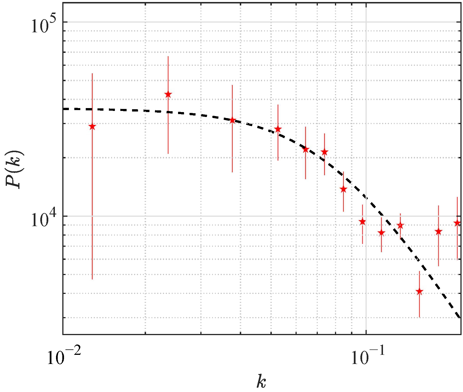
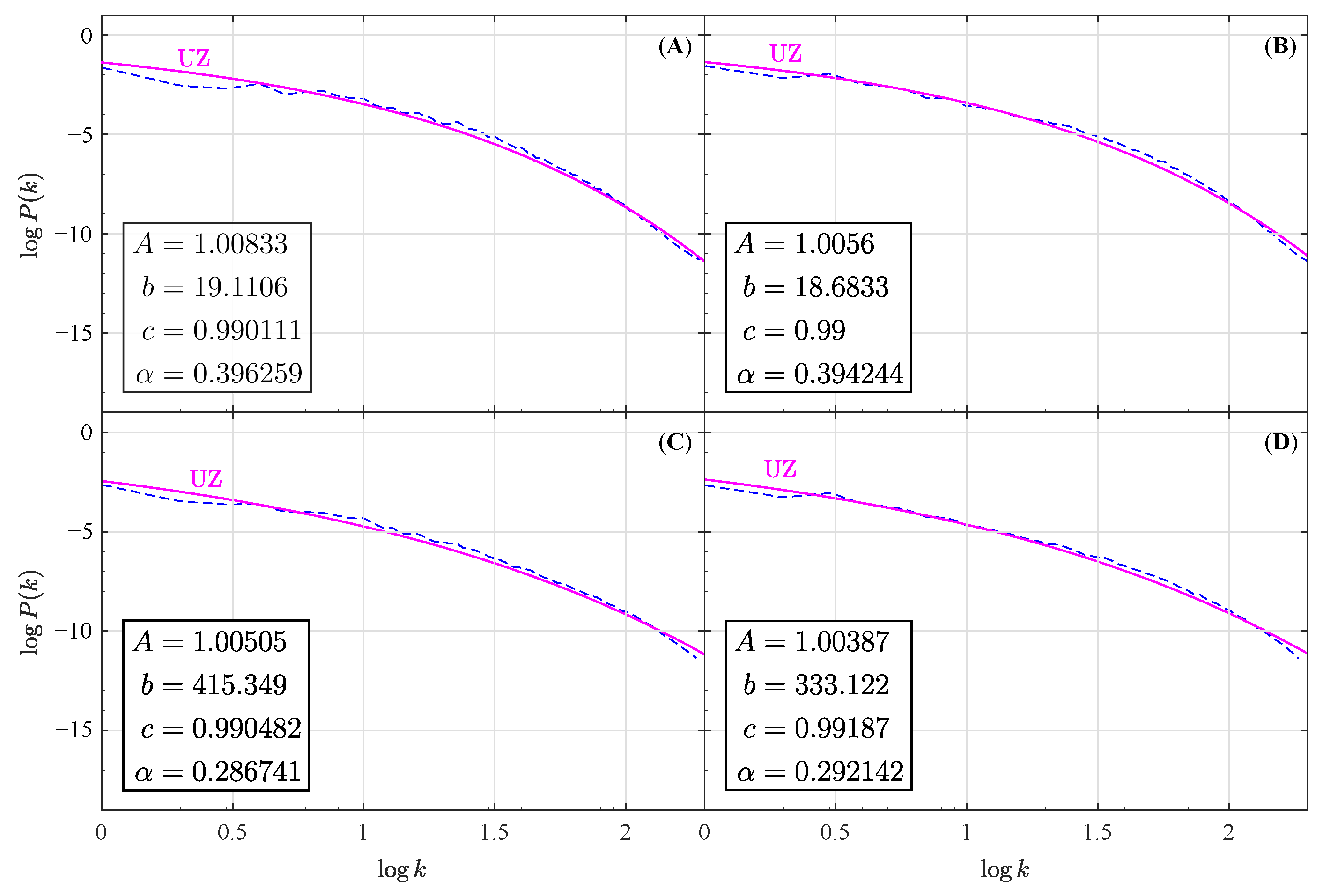
Figure 5 shows the relation to the ISM power spectra of the numerically generated three-dimensional MHD-turbulence by using the MHD code [32] and varying the input values for the sonic and Alfvénic Mach numbers that were presented in [33]. Figure 5A relates to the power spectra line with a greater Alfvénic-Mach number and the thick case of varying abundances; Figure 5B is the same with a lower Alfvénic-Mach number and the thick case; Figure 5C is the same with a greater Alfvénic-Mach number and the normal case; Figure 5D is same with a greater Alfvénic-Mach number and the normal case. This time, the quality of the UZ approximation is more than satisfactory.

9. Conclusions

In its mathematical essence, a cloud model of a medium differs from a smooth (wave) one in its discreteness, remaining in this respect similar to a lattice model, which, however, has a special property—the stochasticity in the nodes’ spatial arrangement. In particular, such a model was used in the works [22,34] and described in the book [35].

Here are its main positions:

(1) Involving the cloud model in the consideration of CR diffusion and the fragmentation problem, the authors of [22] indicated the strong ISM clumping as a significant factor influencing these processes, but completely ignored the cloud correlations, assuming that the averaged diffusion equation may be written (in conventional notation) as:

$$-\nabla \langle D\nabla N\rangle +v\sigma \langle nN\rangle =\langle Q\rangle ,$$

(10)

where $\langle ...\rangle$ means averaging over a statistical ensemble, which is assumed to be the Poissonian ensemble (no other indications given) [22]. This seems to be the most controversial assumption of this model, since numerous observational data point to a hierarchical type of inhomogeneity, being inconsistent with a uniform Poisson distribution.

The theoretical basis for the simulation of the random point distributions with power-type spatial correlations was developed in [11], and some technical details can be found in [15] (see also [10], Chapter 8). Chapter 5 in [17] contains the validation of the replacement in the CR diffusion equation:

$$-\nabla \langle D\nabla N\rangle \mapsto -K_{\alpha }{(-\Delta )}^{\alpha /2}$$

(11)

when coming from Poissonian to the Lévy–Feldheim statistical ensemble for the cloud distribution of the ISM. The most intriguing information about the fractional Laplacian and other fractional analysis operators can be found in the two-volume handbook [19]. A time-dependent version of the fractional modification of the CR transport equation was introduced in [36] and extensively analyzed by L. Dorman in his encyclopedic monograph on cosmic rays [37];

(2) More information can be obtained from the structure function, calculated for the mesofractal medium (Figure 6). The structure function shows the conditional density of objects (in this case, molecular clouds) at a distance r from a randomly selected object. It can be seen that the nearest neighbors are distributed according to the fractal law, while the distribution of distant neighbors decreases according to the exponential law. As the point of mode change (crossover), the point of intersection of two asymptotes is chosen, the coordinate of which is determined by the formula:

$$r_0=b{A}_0^{1/(3-\alpha )}.$$

(12)

In the mesofractal terminology1, a sphere of radius $r_0$ separates the fractal and uniform phases, but from a probabilistic point of view, it separates the correlated medium contained inside the sphere from the uncorrelated medium, consisting of objects independently located relative to each other. The free path distribution in the fractal phase has a power-law form and in a uniform phase follows the exponential law.

Applying Equation (12) to the case presented in Figure 5A, we calculated $r_0\approx 20\mathrm{pc}$ and plot the result in Figure 6. By order of magnitude, this value does not conflict with the common representation [2,5,22];

(3) The conclusion, following our calculations, concerns F. Combes’ assumption [3] regarding the similarity of the distribution of galaxies in the Universe and interstellar clouds in the Galaxy. Now, we can say that the similarity takes place not only in a qualitative fractal (that is, due to the coincidence of fractal dimensions) sense, but is also quantitatively characterized by a common structural four-parameter spectral function, directly related to the Ornstein–Zernike equation—one of the most important equations of statistical mechanics;

(4) The authors of [38] combined new Parkes telescope observations of neutral hydrogen (Hı) in the Small Magellanic Cloud (SMC) with an Australia Telescope Compact Array (ATCA) aperture synthesis mosaic to obtain a set of images sensitive to all angular (spatial) scales between 98 arcsec (30 pc) and 48 arcsec (4 kpc). The spatial power spectrum closely obeys the relation $P\left(k\right)\propto k^{-\gamma }$, with $\gamma \approx 3$. The authors’ interpretation was that the interstellar medium (ISM) of the SMC is fractal in nature, consisting of a hierarchy of Hı cloud structures created, for example, by homogeneous turbulence. The projected fractal dimension of $D_p\approx 1.5$ is similar to the values obtained by other authors for molecular clouds in the Galaxy in the size range of $0.05÷100$ pc. Such a model is consistent with a low space-filling factor for the neutral gas, and the image of it is shown on Figure 7A. Figure 7B shows an image of an ISM fragment containing three distinct clusters of molecular clouds. It is worth emphasizing that their formation itself was in no way provoked by the computer code, which built independent random trajectories from independent random segments. The appearance of clusters against the background of a uniform Poisson field of seed nodes is a consequence of the statistical feature of Lévy walks. Nevertheless, on both pairs of drawings, some common features are visible, not the sizes and arrangements of similar parts, but some commonality of their configurations.

Figure 8 shows a similar situation, but for the galaxies, not for clouds. On the left side, there are $B{z}^{\prime }K$ images of the central 1 Mpc region of clusters spanning the redshift range of detections. This is an image from the cluster catalog extracted from the UKIRT Infrared Deep Sky Survey (UKIDSS) Early Data Release [39,40].

Comparing Figure 2 from [9] with Figure 1 from [41], we see, that not just galaxies, but molecular clouds and young stars are characterized by the spatial distribution, relating to the UZ power spectrum and, as a result, revealing its mesofractal structure. This, in particular, means that the CR-transport process, following at small scales an anomalous diffusion model, turns into the normal diffusion at large scales.

We supposed that the results demonstrated in the paper unequivocally give positive answers to the first two questions. The amazing similarity observed between such different scales and the material composition as the Galaxy and the Universe, of course, has a physical explanation, but such a reproduction of the structures described by non-local models can hardly be considered an ordinary phenomenon.

References

- von Weizsäcker, C.F. The Evolution of Galaxies and Stars. Astrophys. J. 1951, 114, 165. [Google Scholar] [CrossRef]
- Fermi, E. On the Origin of the Cosmic Radiation. Phys. Rev. 1949, 75, 1169–1174. [Google Scholar] [CrossRef]
- Combes, F. Fractal Structures Driven by Self-gravity: Molecular Clouds and the Universe. Celest. Mech. Dyn. Astron. 1998, 72, 91–127. [Google Scholar] [CrossRef] [Green Version]
- Combes, F. Astrophysical fractals: Interstellar medium and galaxies. Adv. Ser. Astrophys. Cosmol. 2000, 10, 143–172. [Google Scholar] [CrossRef] [Green Version]
- Dudorov, A.E. Properties of the hierarchy of interstellar magnetic clouds. Sov. Astron. 1991, 35, 342. [Google Scholar]
- Scalo, J.M. Fragmentation and Hierarchical Structure in the Interstellar Medium; University of Arizona Press: Tucson, AZ, USA, 1985. [Google Scholar]
- Baryshev, Y.; Sylos Labini, F.; Montuori, M.; Pietronero, L. Facts and ideas in modern cosmology. Vistas Astron. 1994, 38, 419–500. [Google Scholar] [CrossRef] [Green Version]
- Baryshev, Y.; Teerikorpi, P.; Mandelbrot, B. Discovery of Cosmic Fractals; World Scientific: Singapore, 2002. [Google Scholar] [CrossRef]
- Uchaikin, V.V.; Litvinov, V.A.; Kozhemyakina, E.V.; Kozhemyakin, I.I. A Random Walk Model for Spatial Galaxy Distribution. Mathematics 2021, 9, 98. [Google Scholar] [CrossRef]
- Uchaikin, V.V.; Zolotarev, V.M. Chance and Stability: Stable Distributions and Their Applications; Walter de Gruyter: Berlin, Germany, 1999. [Google Scholar]
- Uchaikin, V.V.; Gusarov, G.G. Lévy flight applied to random media problems. J. Math. Phys. 1997, 38, 2453–2464. [Google Scholar] [CrossRef]
- Uchaikin, V.; Korobko, D.; Gismyatov, I. Modified Mandelbrot algorithm for stochastic analysis of a fractal-type distribution of galaxies. Russ. Phys. J. 1997, 40, 711–716. [Google Scholar] [CrossRef]
- Uchaikin, V.; Gismjatov, I.; Gusarov, G.; Svetukhin, V. Paired Lévy-Mandelbrot Trajectory as a Homogeneous Fractal. Int. J. Bifurc. Chaos 1998, 8, 965–984. [Google Scholar] [CrossRef]
- Uchaikin, V.V.; Saenko, V.V. Simulation of Random Vectors with Isotropic Fractional Stable Distributions and Calculation of Their Probability Density Functions. J. Math. Sci. 2002, 112, 4211–4228. [Google Scholar] [CrossRef]
- Uchaikin, V. Mathematical modeling of the distribution of galaxies in the universe. J. Math. Sci. 1997, 84, 1175–1178. [Google Scholar] [CrossRef]
- Uchaikin, V. If the Universe were a Lévy-Mandelbrot fractal. Gravit. Cosmol. 2004, 10, 5–24. [Google Scholar]
- Uchaikin, V.; Sibatov, R. Fractional Kinetics in Space; World Scientific: Singapore, 2018. [Google Scholar] [CrossRef]
- Kolmogorov, A. The local structure of turbulence in incompressible viscous fluid for very large Reynolds’ numbers. Akad. Nauk SSSR Dokl. 1941, 30, 301–305. [Google Scholar]
- Uchaikin, V.V. Fractional Derivatives for Physicists and Engineers; Nonlinear Physical Science; Springer: Berlin/Heidelberg, Germany, 2013. [Google Scholar] [CrossRef] [Green Version]
- Giacalone, J.; Jokipii, J.R. The Transport of Cosmic Rays across a Turbulent Magnetic Field. Astrophys. J. 1999, 520, 204–214. [Google Scholar] [CrossRef]
- Ballesteros-Paredes, J.; André, P.; Hennebelle, P.; Klessen, R.; Kruijssen, D.; Chevance, M.; Nakamura, F.; Adamo, A.; Vázquez-Semadeni, E. From Diffuse Gas to Dense Molecular Cloud Cores. Space Sci. Rev. 2020, 216, 76. [Google Scholar] [CrossRef]
- Osborne, J.L.; Ptuskin, V.S. Cosmic rays in the inner galaxy and the diffusion properties of the interstellar medium. Sov. Astron. Lett. 1987, 13, 413. [Google Scholar] [CrossRef] [Green Version]
- Mandelbrot, B.B. The Fractal Geometry of Nature; W.H. Freeman: San Francisco, CA, USA, 1982. [Google Scholar]
- Peebles, P. The Large-Scale Structure of the Universe; Princeton Series in Physics; Princeton University Press: Princeton, NJ, USA, 1980. [Google Scholar]
- Borgani, S. Scaling in the Universe. Phys. Rep. 1995, 251, 1–152. [Google Scholar] [CrossRef]
- Mandelbrot, B.B. The Fractal Range of the Distribution of Galaxies, Crossover to Homogeneity, and Multifractals. In Large Scale Structure and Motions in the Universe, Proceedings of the International Meeting, Trieste, Italy, 6–9 April 1988; Mezzetti, M., Giuricin, G., Mardirossian, F., Ramella, M., Eds.; Springer: Dordrecht, The Netherlands, 1989; pp. 259–279. [Google Scholar] [CrossRef]
- Uchaikin, V.V. The mesofractal universe driven by Rayleigh-Lévy walks. Gen. Relativ. Gravit. 2004, 36, 1689–1717. [Google Scholar] [CrossRef]
- Stell, G. Statistical mechanics applied to random-media problems. Lect. Appl. Math. 1991, 27, 109–137. [Google Scholar]
- Frisch, U. Turbulence: The Legacy of A.N. Kolmogorov; Cambridge University Press: Cambridge, UK, 1995. [Google Scholar] [CrossRef]
- Percival, W.J.; Baugh, C.M.; Bland-Hawthorn, J.; Bridges, T.; Cannon, R.; Cole, S.; Colless, M.; Collins, C.; Couch, W.; Dalton, G.; et al. The 2dF Galaxy Redshift Survey: The power spectrum and the matter content of the Universe. Mon. Not. R. Astron. Soc. 2001, 327, 1297–1306. [Google Scholar] [CrossRef]
- Percival, W.J.; Burkey, D.; Heavens, A.; Taylor, A.; Cole, S.; Peacock, J.A.; Baugh, C.M.; Bland-Hawthorn, J.; Bridges, T.; Cannon, R.; et al. The 2dF Galaxy Redshift Survey: Spherical harmonics analysis of fluctuations in the final catalog. Mon. Not. R. Astron. Soc. 2004, 353, 1201–1218. [Google Scholar] [CrossRef] [Green Version]
- Cho, J.; Lazarian, A. Compressible magnetohydrodynamic turbulence: Mode coupling, scaling relations, anisotropy, viscosity-damped regime and astrophysical implications. Mon. Not. R. Astron. Soc. 2003, 345, 325–339. [Google Scholar] [CrossRef] [Green Version]
- Burkhart, B.; Lazarian, A.; Ossenkopf, V.; Stutzki, J. The turbulence power spectrum in optically thick interstellar clouds. Astrophys. J. 2013, 771, 123. [Google Scholar] [CrossRef] [Green Version]
- Ptuskin, V.S.; Soutoul, A. Cosmic rays in the cloudy interstellar medium—Production of secondary nuclei. Astron. Astrophys. 1990, 237, 445–453. [Google Scholar]
- Berezinskii, V.S.; Bulanov, S.V.; Dogiel, V.A.; Ptuskin, V.S. Astrophysics of Cosmic Rays; North Holland: Amsterdam, The Netherlands, 1990. [Google Scholar]
- Lagutin, A.; Nikulin, Y.; Uchaikin, V. The “knee” in the primary cosmic ray spectrum as consequence of the anomalous diffusion of the particles in the fractal interstellar medium. Nucl. Phys. B-Proc. Suppl. 2001, 97, 267–270. [Google Scholar] [CrossRef]
- Dorman, L. Cosmic Ray Interactions, Propagation, and Acceleration in Space Plasmas; Springer: Dordrecht, The Netherlands, 2006; Volume 339. [Google Scholar] [CrossRef] [Green Version]
- Stanimirović, S.; Staveley-Smith, L.; Dickey, J.M.; Sault, R.J.; Snowden, S.L. The large-scale Hıstructure of the Small Magellanic Cloud. Mon. Not. R. Astron. Soc. 1999, 302, 417–436. [Google Scholar] [CrossRef]
- Lawrence, A.; Warren, S.J.; Almaini, O.; Edge, A.C.; Hambly, N.C.; Jameson, R.F.; Lucas, P.; Casali, M.; Adamson, A.; Dye, S.; et al. The UKIRT Infrared Deep Sky Survey (UKIDSS). Mon. Not. R. Astron. Soc. 2007, 379, 1599–1617. [Google Scholar] [CrossRef] [Green Version]
- van Breukelen, C.; Clewley, L.; Bonfield, D.G.; Rawlings, S.; Jarvis, M.J.; Barr, J.M.; Foucaud, S.; Almaini, O.; Cirasuolo, M.; Dalton, G.; et al. Galaxy clusters at 0.6 < z < 1.4 in the UKIDSS Ultra Deep Survey Early Data Release. Mon. Not. R. Astron. Soc. Lett. 2006, 373, L26–L30. [Google Scholar] [CrossRef] [Green Version]
- Kraus, A.L.; Hillenbrand, L.A. Spatial Distributions of Young Stars. Astrophys. J. 2008, 686, L111. [Google Scholar] [CrossRef] [Green Version]
Figure 1.
Qualitative sketches of CR particle trajectories in two different models. (A)—in the wave model; (B)—in the cloud model ( are free path distribution indices, are clouds diameters).
Figure 2.
Fractal (a), mesofractal (b), and uniform Poisson set (c) (Monte Carlo simulations).
Figure 3.
2dFGRS galaxy power spectrum [30] (dots) and its UZ approximation (dashed line) with A = 586.21, b = 1.22808, c = 0.99, α = 1.53515. Adapted with permissions from IOP Publishing [30]. Copyright 2001 IOP Publishing.
Figure 4.
Same as in Figure 3 for data from [31] with A = 35.9332, b = 0.882462, c = 0.999, α = 2.58324. Adapted with permissions from IOP Publishing [31]. Copyright 2004 IOP Publishing.
Figure 5.
Power spectra approximations of ISM data. The blue dashed lines are simulated power spectra from [33]: (A) is the energy spectrum generated MHD simulation with a lower Alfvénic-Mach number and the thick case of varying abundances; (B) is the same with a greater Alfvénic-Mach number and the thick case of varying abundances; (C) is the same with a lower Alfvénic-Mach number and the normal case of varying abundances; (D) is the same with a greater Alfvénic-Mach number and the normal case of varying abundances. The purple lines are the Uchaikin–Zolotarev (UZ) spectrum approximated by function (2). The values of A, b, c, and in the corners are the parameters for the UZ-spectrum (2). Adapted with permissions from Ref. [33]. Copyright 2013 IOP Publishing.
Figure 6.
Structure function with the parameters from Figure 5A. The dashed-dotted line corresponds to the fractal phase of the mesofractal with fractal dimension . The dashed line corresponds to the uniform phase having an exponential distribution. Crossover point is is defined by the intersection of two asymptotes.
Figure 7.
(A) is a Hı image of the Small Magellanic Cloud ([38] Figure 1). Adapted with permissions from Ref. [38]. Copyright 1999 Oxford Journals. (B) is the pattern, by Monte Carlo simulations, with the UZ ansatz for parameters , , . Full circles are the seed node positions of the Markov chains.
Figure 8.
(A) is the image of the central 1 Mpc region of galaxy clusters spanning the redshift range of detections in [40]. Adapted with permissions from Ref. [40]. Copyright 2006 Oxford Journals. (B) is the pattern by Monte Carlo simulations with the UZ ansatz. Full circles are the seed node positions of the Markov chains.
Publisher’s Note: MDPI stays neutral with regard to jurisdictional claims in published maps and institutional affiliations. |
© 2022 by the authors. Licensee MDPI, Basel, Switzerland. This article is an open access article distributed under the terms and conditions of the Creative Commons Attribution (CC BY) license (https://creativecommons.org/licenses/by/4.0/).
Share and Cite
MDPI and ACS Style
Uchaikin, V.V.; Kozhemyakin, I.I. A Mesofractal Model of Interstellar Cloudiness. Universe 2022, 8, 249. https://0-doi-org.brum.beds.ac.uk/10.3390/universe8050249
AMA Style
Uchaikin VV, Kozhemyakin II. A Mesofractal Model of Interstellar Cloudiness. Universe. 2022; 8(5):249. https://0-doi-org.brum.beds.ac.uk/10.3390/universe8050249
Chicago/Turabian StyleUchaikin, Vladimir V., and Ilya I. Kozhemyakin. 2022. "A Mesofractal Model of Interstellar Cloudiness" Universe 8, no. 5: 249. https://0-doi-org.brum.beds.ac.uk/10.3390/universe8050249
Note that from the first issue of 2016, this journal uses article numbers instead of page numbers. See further details here.