Author Contributions
D.D.: conceptualization, supervision, validation, review and editing. G.R.: conceptualization, supervision, validation, review and editing. E.D.: methodology, validation, data curation, review and editing. A.Q.: conceptualization, supervision, validation, review and editing. D.M.: conceptualization, supervision, validation, review and editing. F.A.: formal analysis, data curation, software, writing—original draft, writing—review and editing. All authors have read and agreed to the published version of the manuscript.
Figure 1.
Front roll center variation characteristic.
Figure 1.
Front roll center variation characteristic.
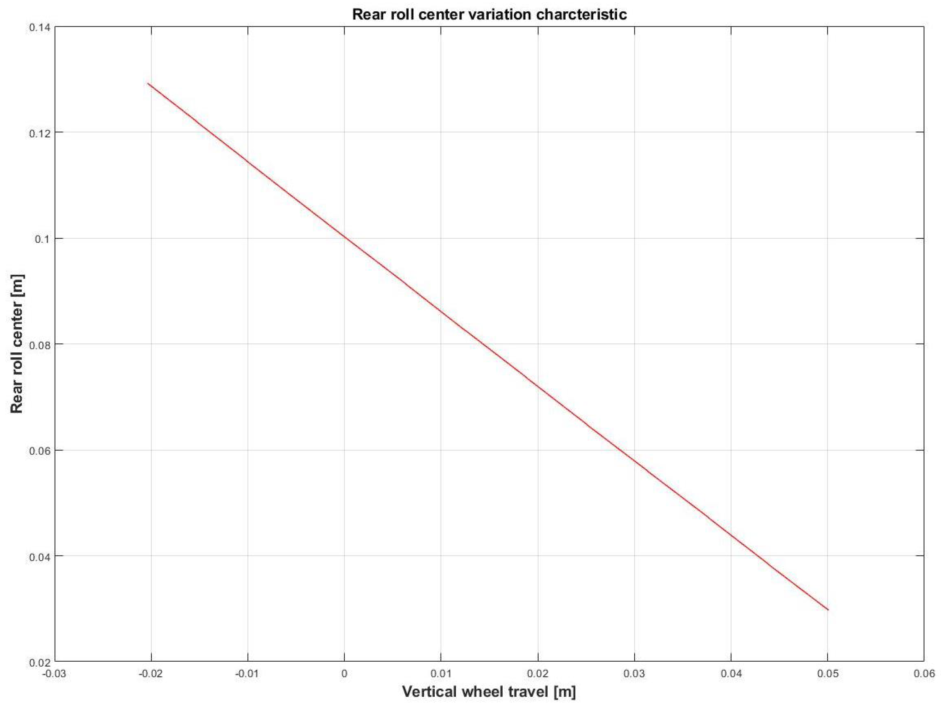
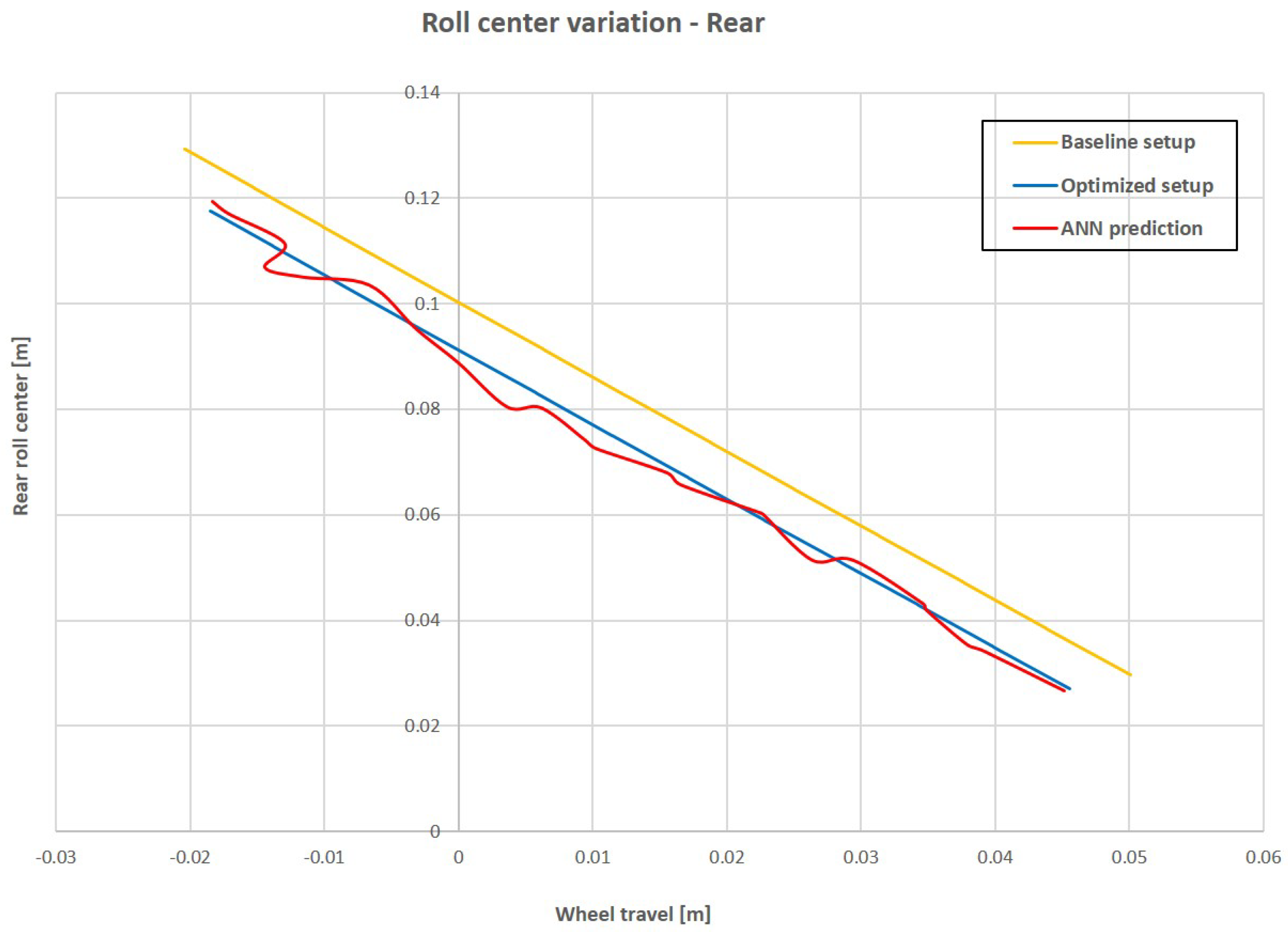
Figure 2.
Rear roll center variation characteristic.
Figure 2.
Rear roll center variation characteristic.
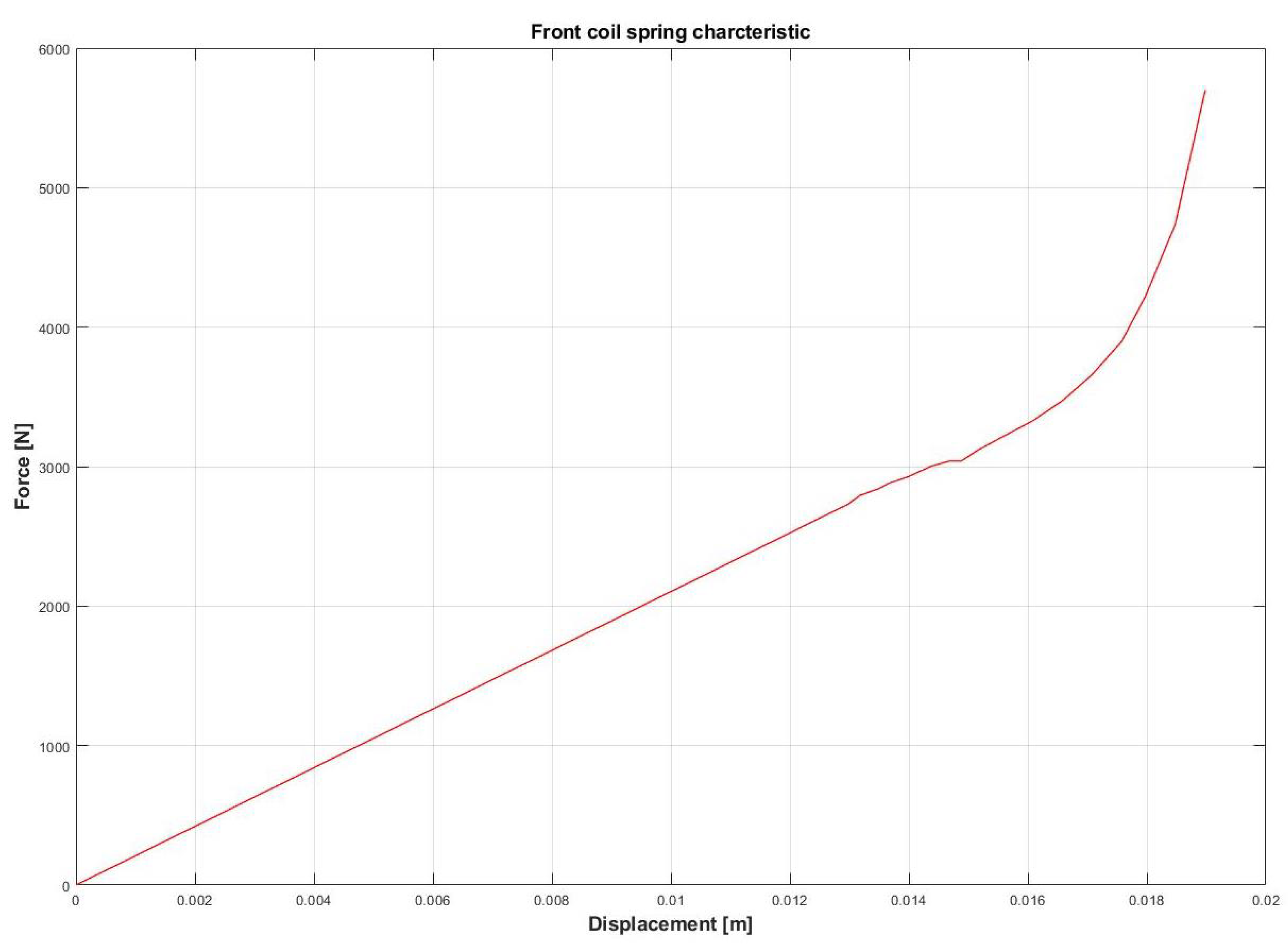
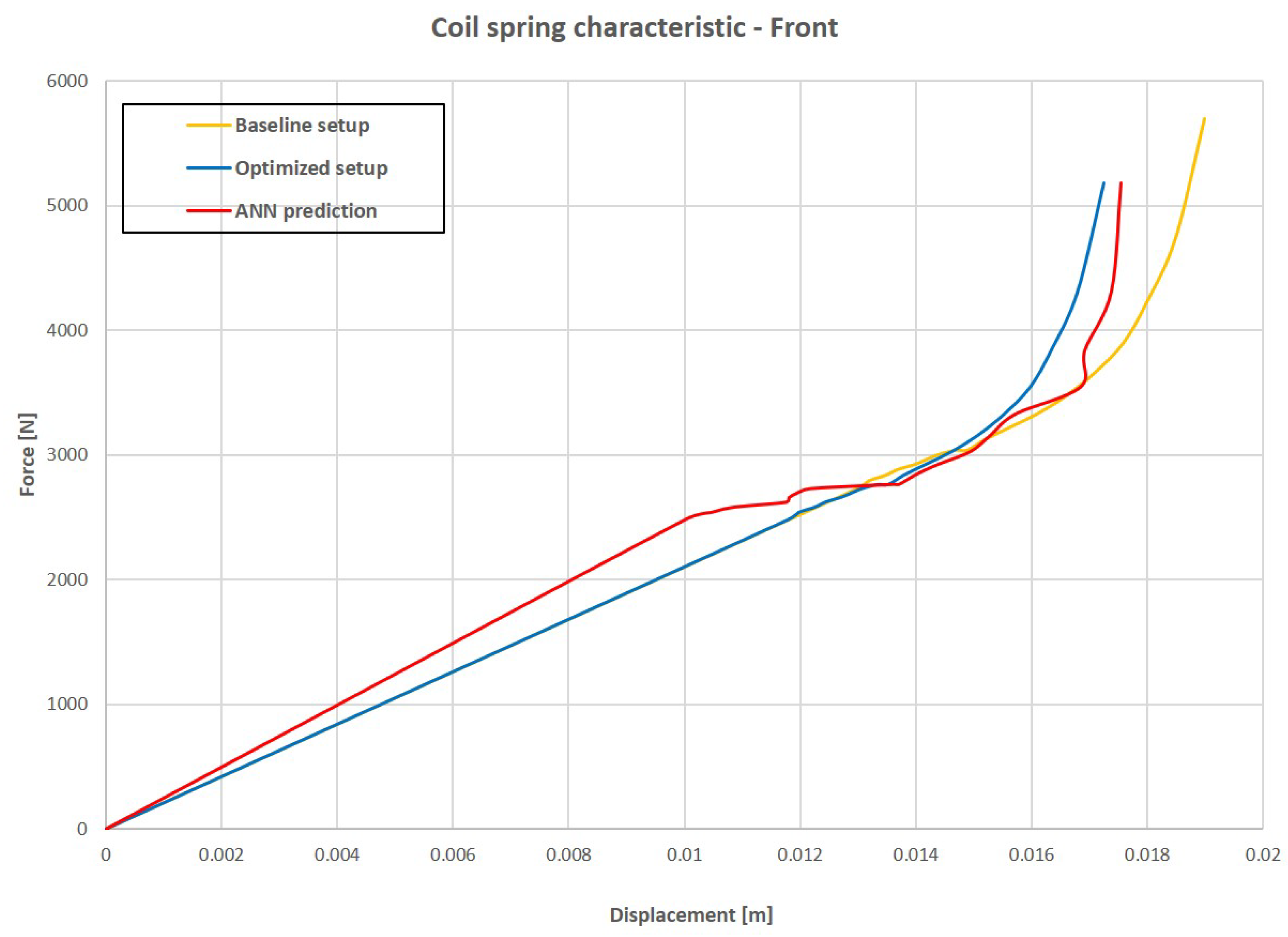
Figure 3.
Front coil spring characteristic.
Figure 3.
Front coil spring characteristic.
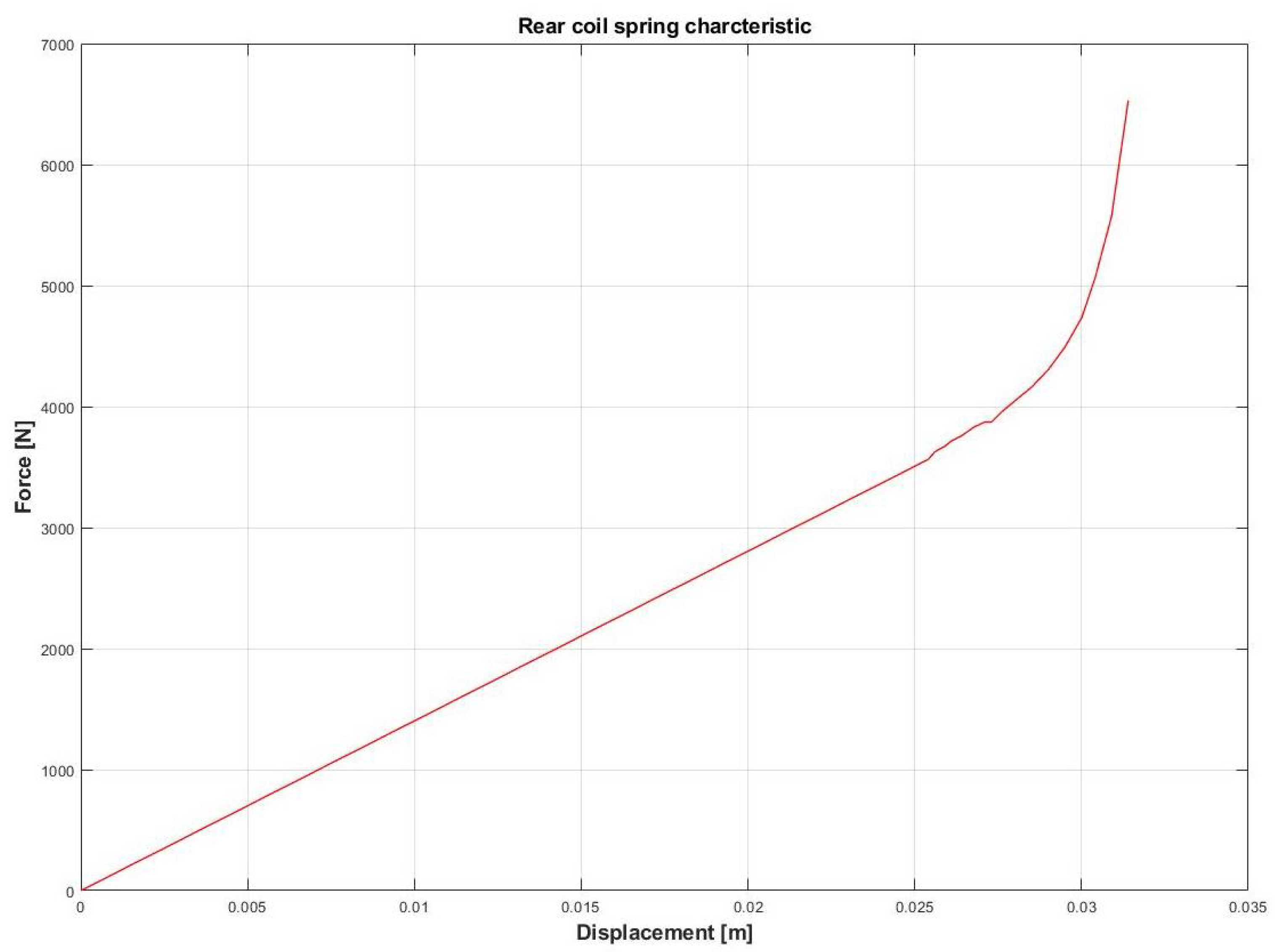
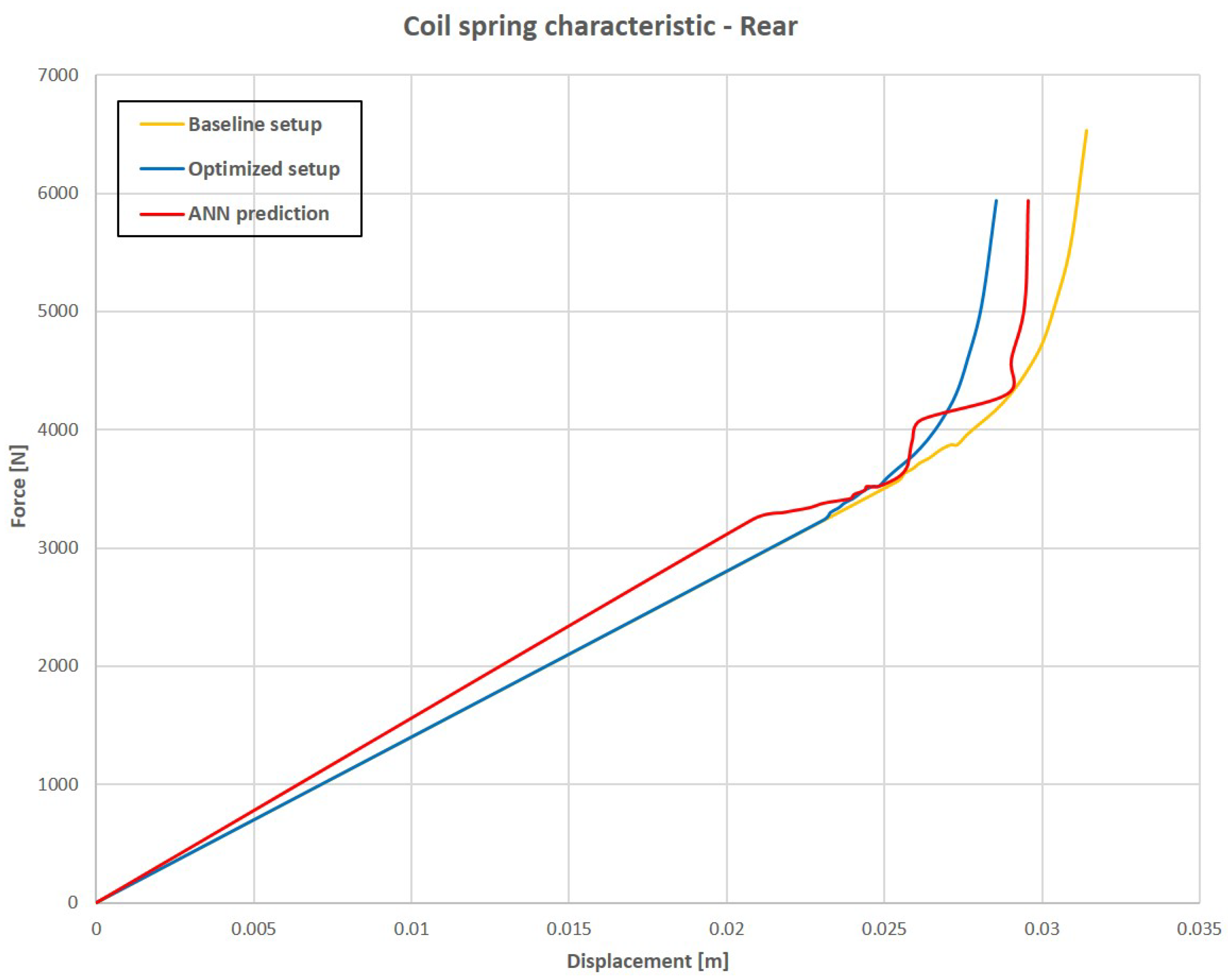
Figure 4.
Rear coil spring characteristic.
Figure 4.
Rear coil spring characteristic.
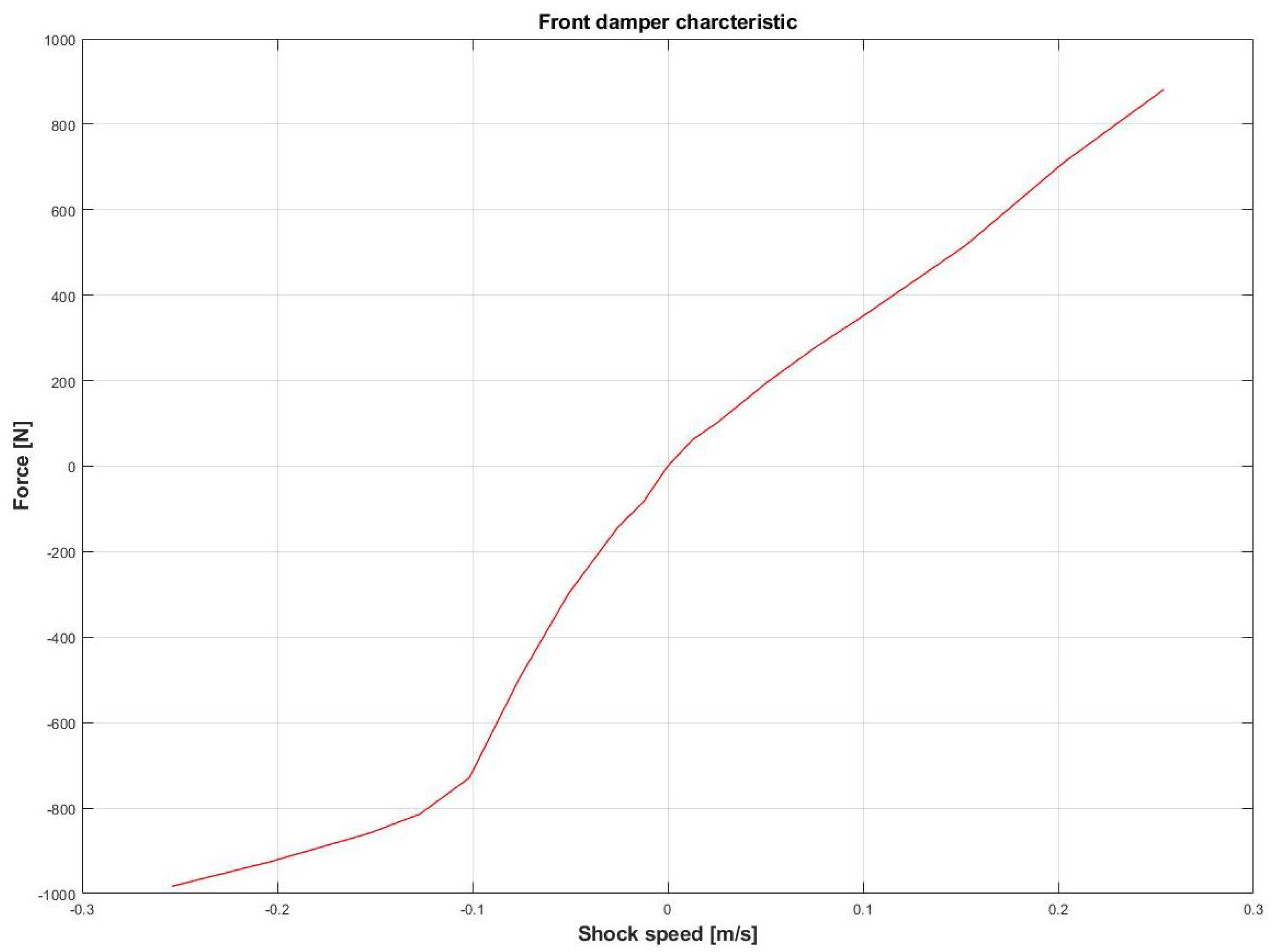
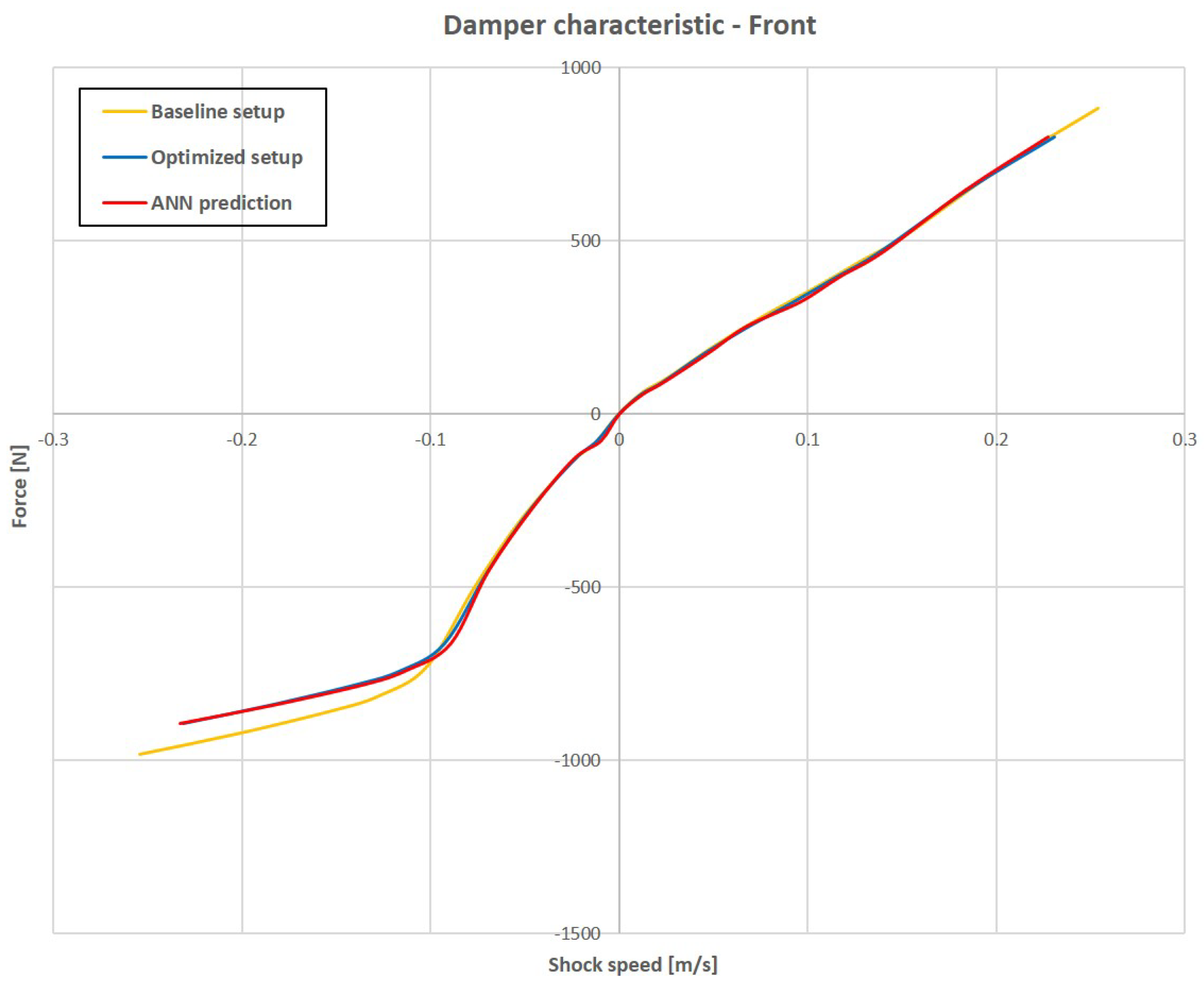
Figure 5.
Front damper characteristic.
Figure 5.
Front damper characteristic.
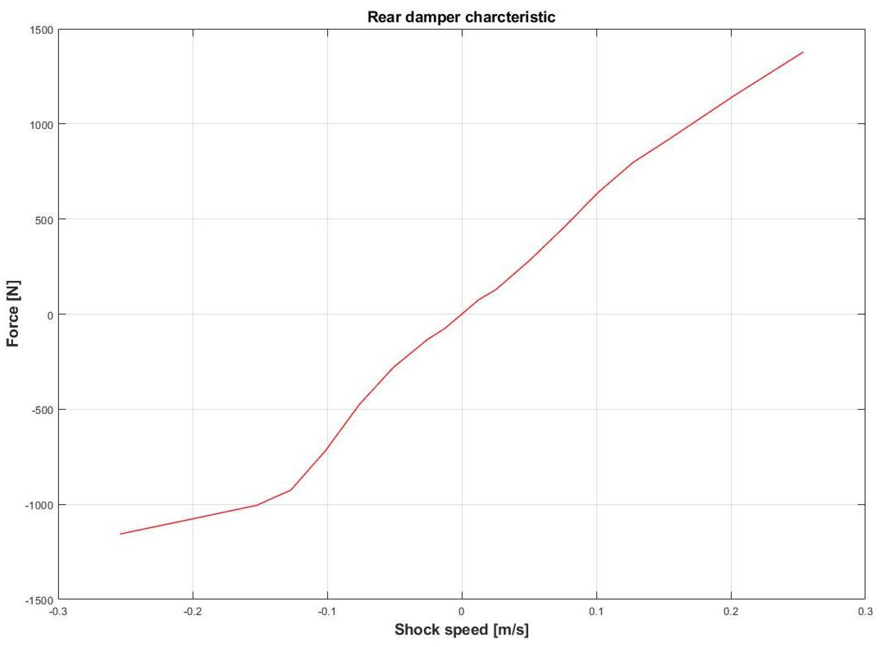
Figure 6.
Rear damper characteristic.
Figure 6.
Rear damper characteristic.
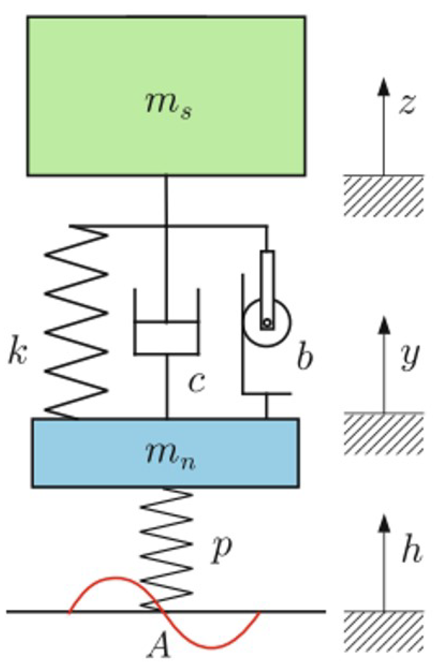
Figure 7.
Quarter Car model.
Figure 7.
Quarter Car model.
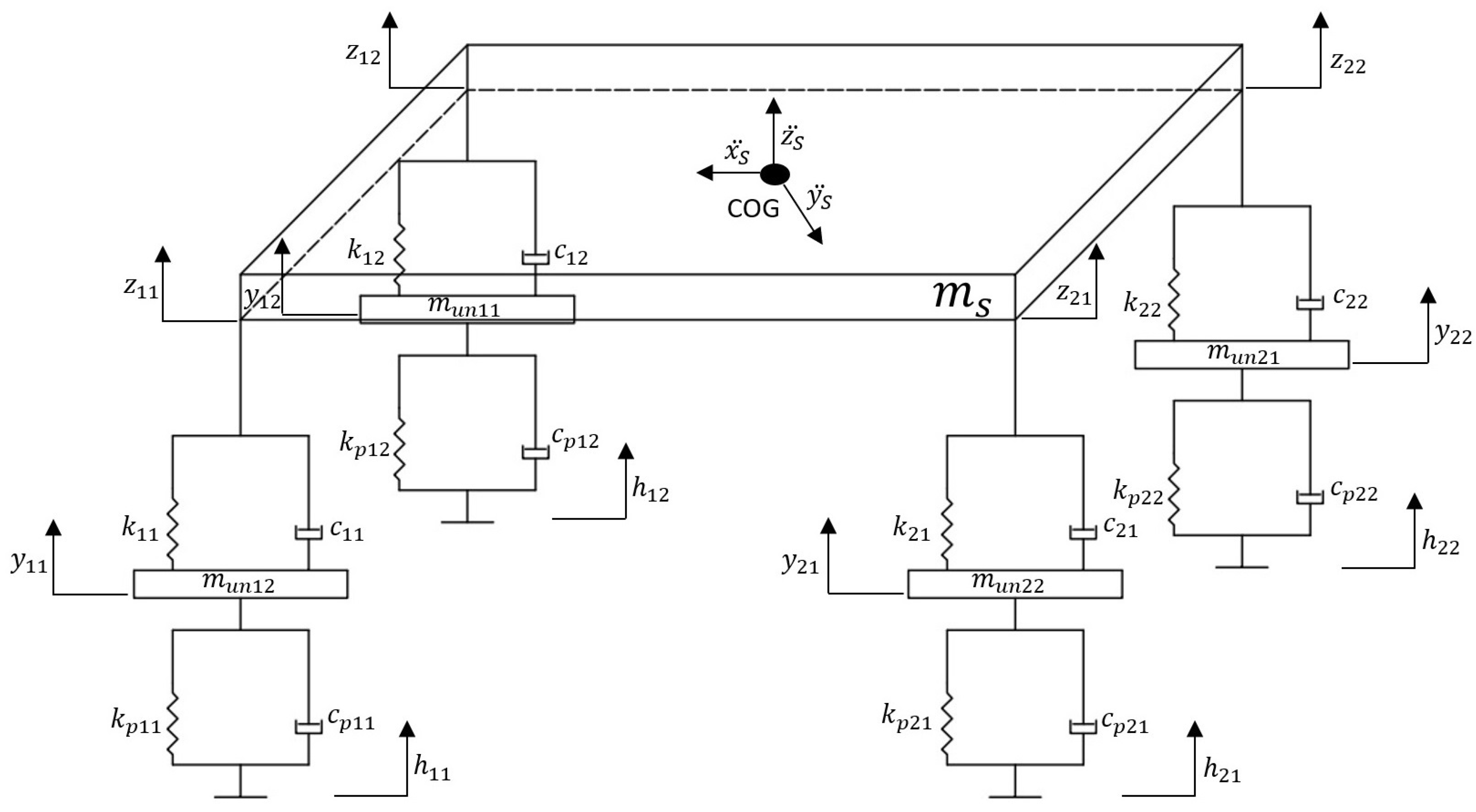
Figure 8.
7-DOF mathematical model.
Figure 8.
7-DOF mathematical model.
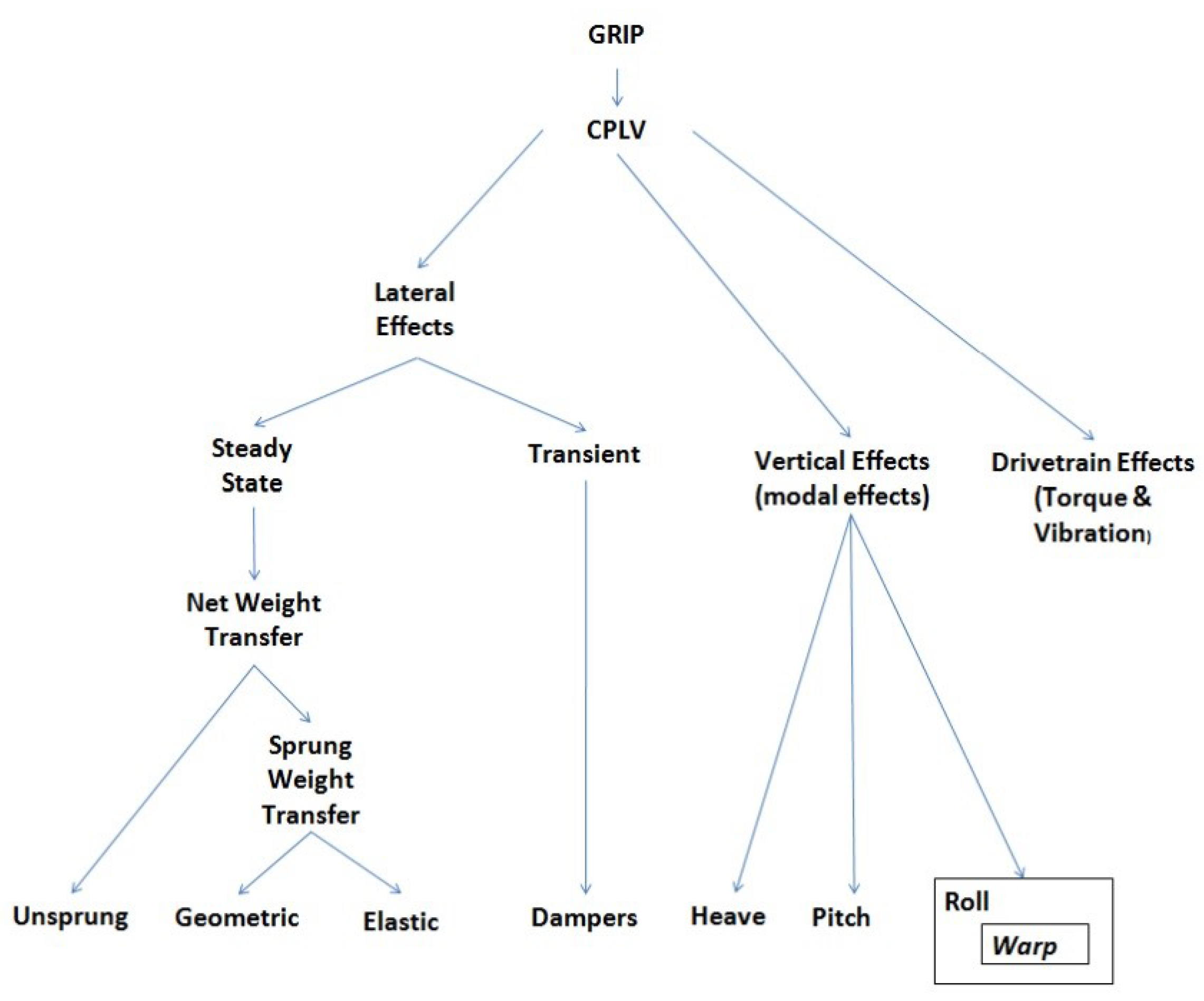
Figure 9.
The performance of the vehicle is related to the grip between road and tire. Improving the grip means decreasing the CPLV, which depends on weight transfer and body movements of roll, pitch and heave.
Figure 9.
The performance of the vehicle is related to the grip between road and tire. Improving the grip means decreasing the CPLV, which depends on weight transfer and body movements of roll, pitch and heave.
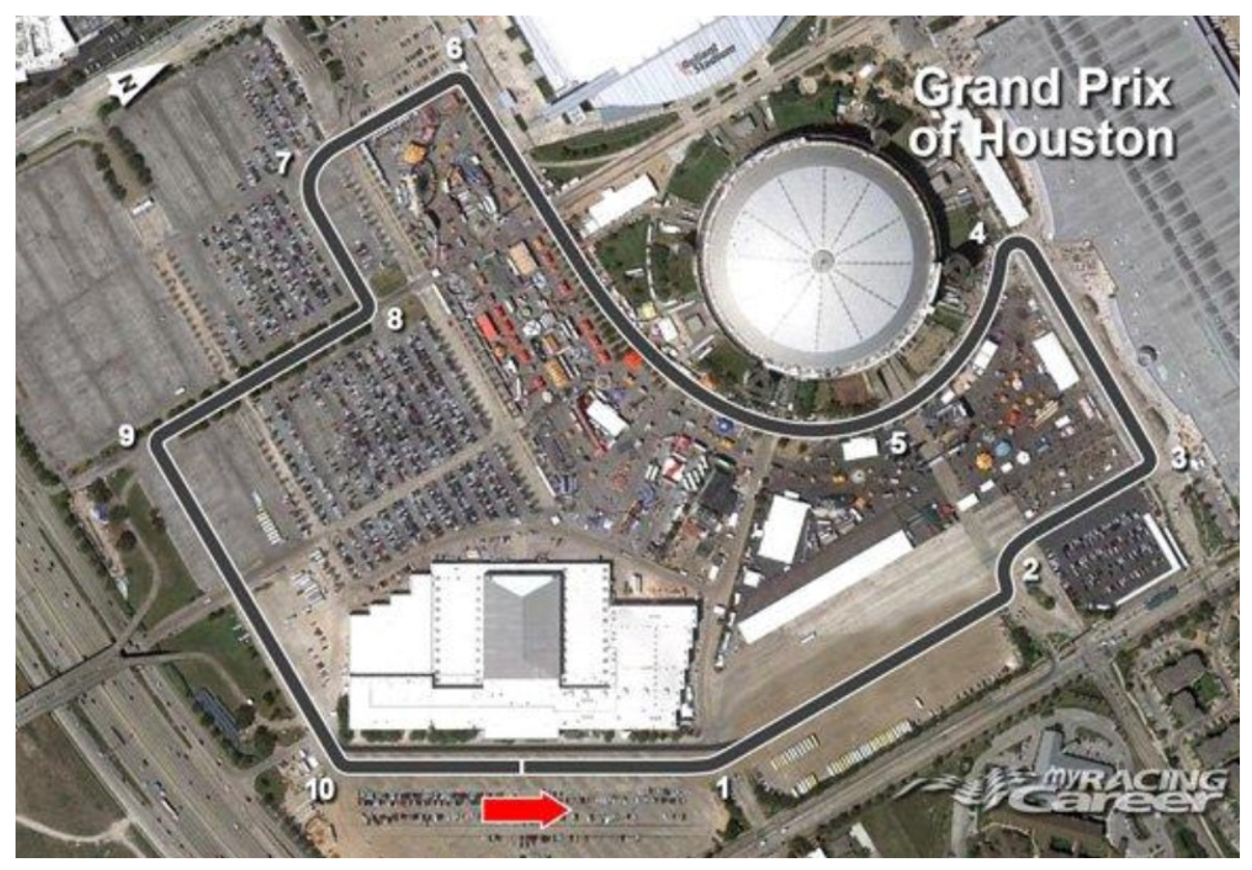
Figure 10.
Houston circuit in Texas, USA.
Figure 10.
Houston circuit in Texas, USA.
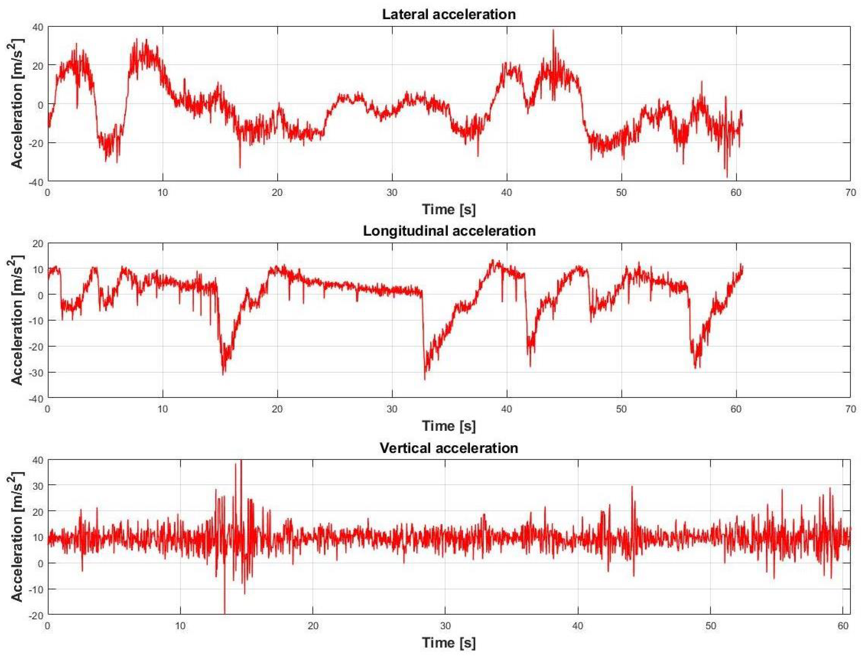
Figure 11.
Lateral, longitudinal and vertical acceleration vs. time.
Figure 11.
Lateral, longitudinal and vertical acceleration vs. time.
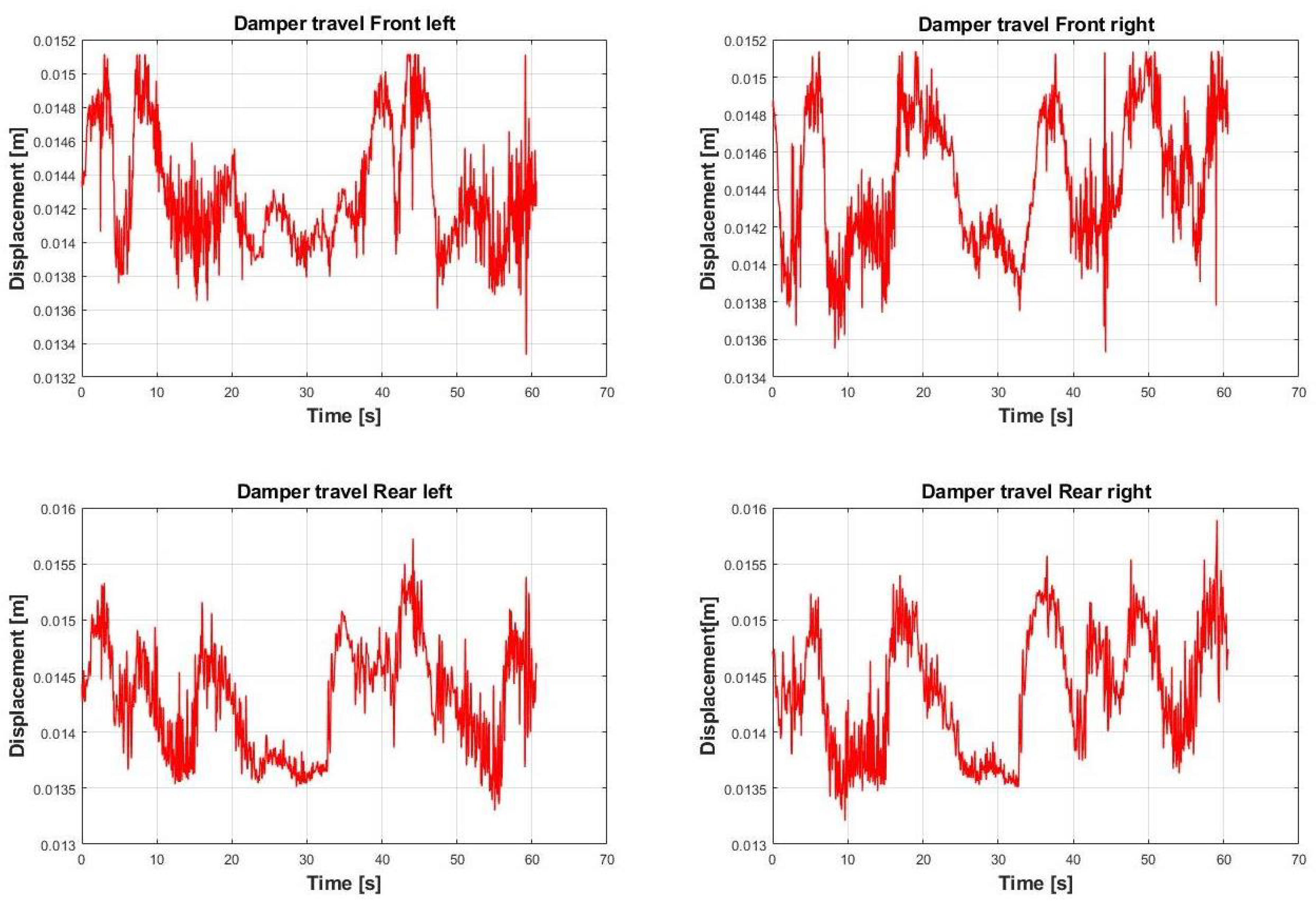
Figure 12.
Damper travels vs. time.
Figure 12.
Damper travels vs. time.
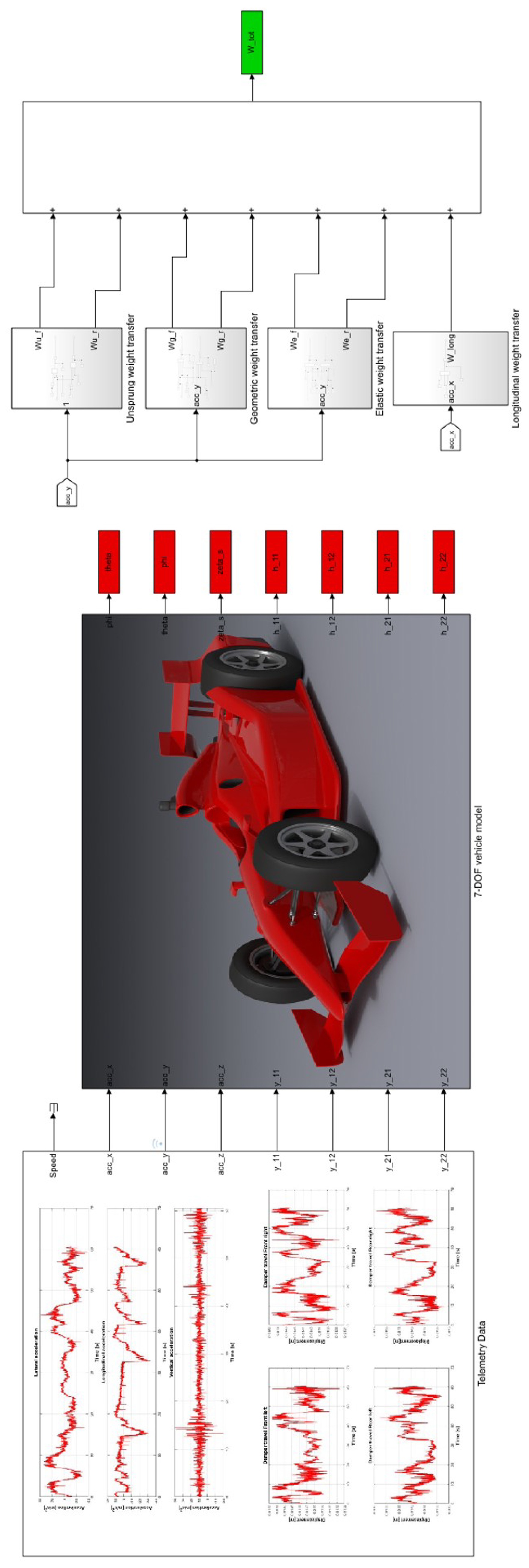
Figure 13.
Simulink model of an IndyCar. Red blocks are the outputs of the model, and the green block is the total weight transfer.
Figure 13.
Simulink model of an IndyCar. Red blocks are the outputs of the model, and the green block is the total weight transfer.
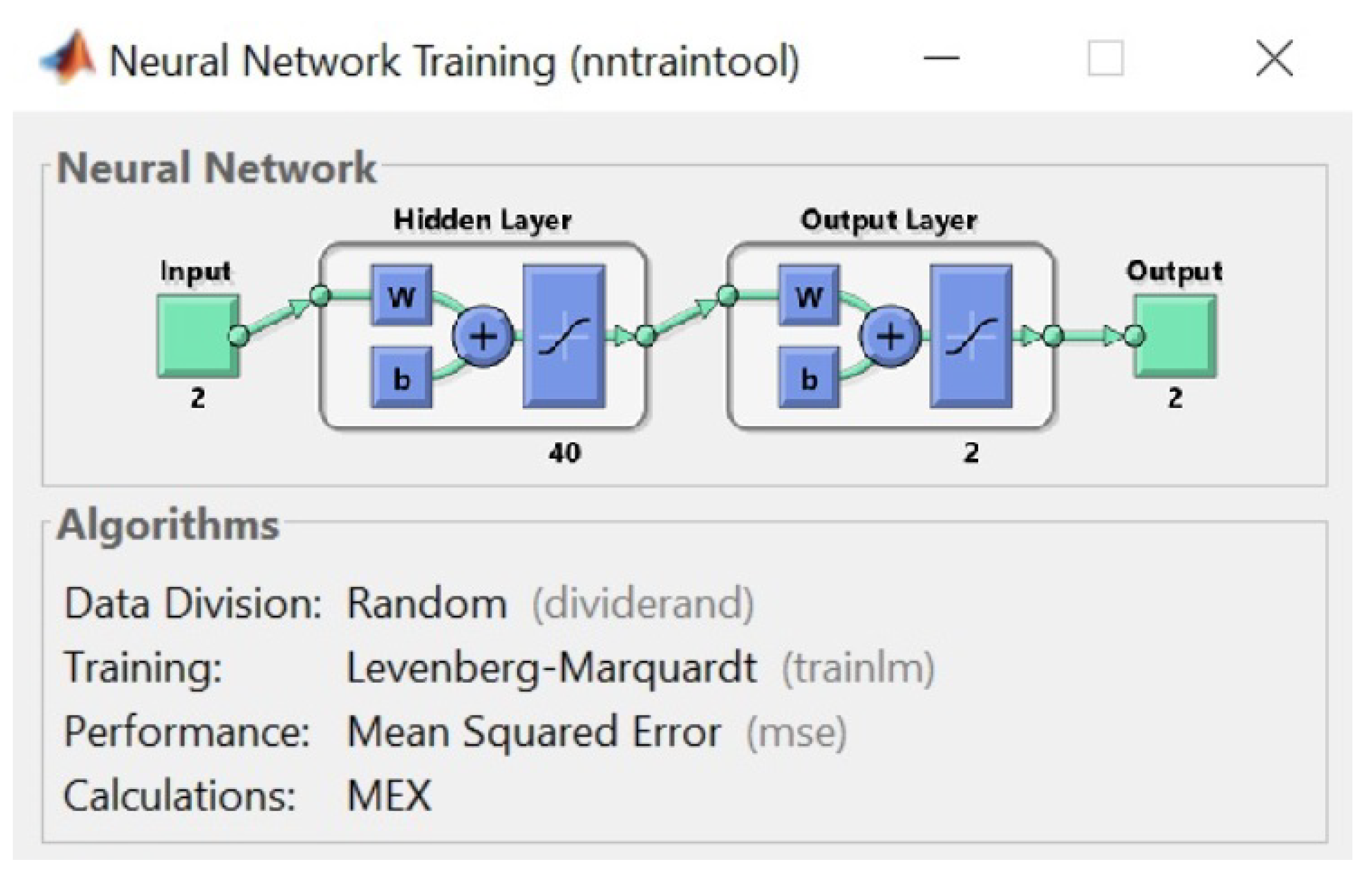
Figure 14.
ANN topology for the Quarter Car model optimization. Input layer contains suspension travel and tire deflection population. The output layer contains the designated variables of the optimization, spring rate and damping rate. The hidden layer contains the artificial neurons.
Figure 14.
ANN topology for the Quarter Car model optimization. Input layer contains suspension travel and tire deflection population. The output layer contains the designated variables of the optimization, spring rate and damping rate. The hidden layer contains the artificial neurons.
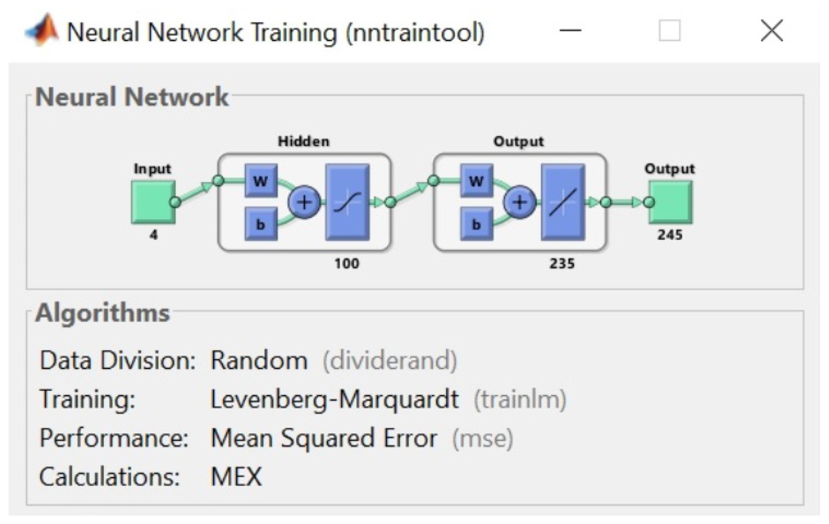
Figure 15.
The ANN topology for the 7-DOF model optimization. The input layer contains the variable to optimize: roll angle, pitch angle, sprung mass vertical travel and total weight transfer. The output layer contains the vectors of the designated variables of the optimization. The hidden layer contains the artificial neuron.
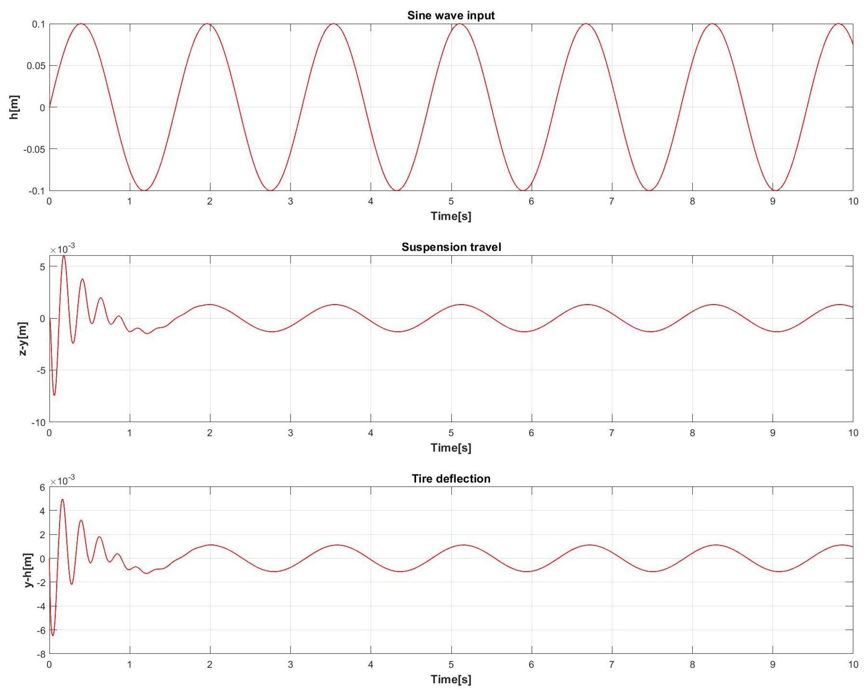
Figure 16.
Quarter Car model response in terms of suspension travel and tire deflection to a sine wave input of 0.1 m of amplitude for a 10 s simulation time.
Figure 16.
Quarter Car model response in terms of suspension travel and tire deflection to a sine wave input of 0.1 m of amplitude for a 10 s simulation time.
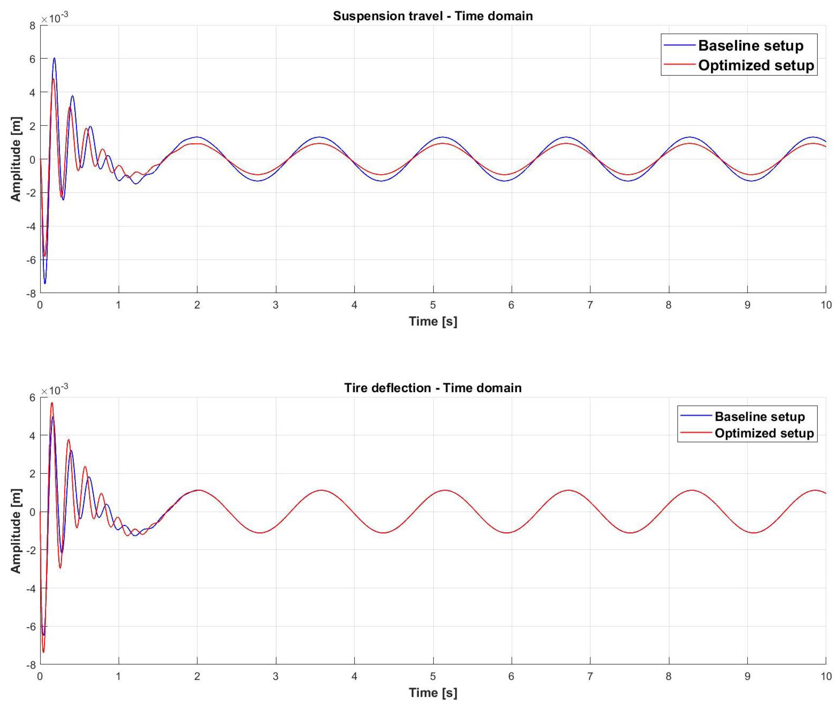
Figure 17.
Comparison between baseline setup and optimized setup. The optimized setup is able to reduce the amplitude of suspension travel and tire deflection in the time domain.
Figure 17.
Comparison between baseline setup and optimized setup. The optimized setup is able to reduce the amplitude of suspension travel and tire deflection in the time domain.
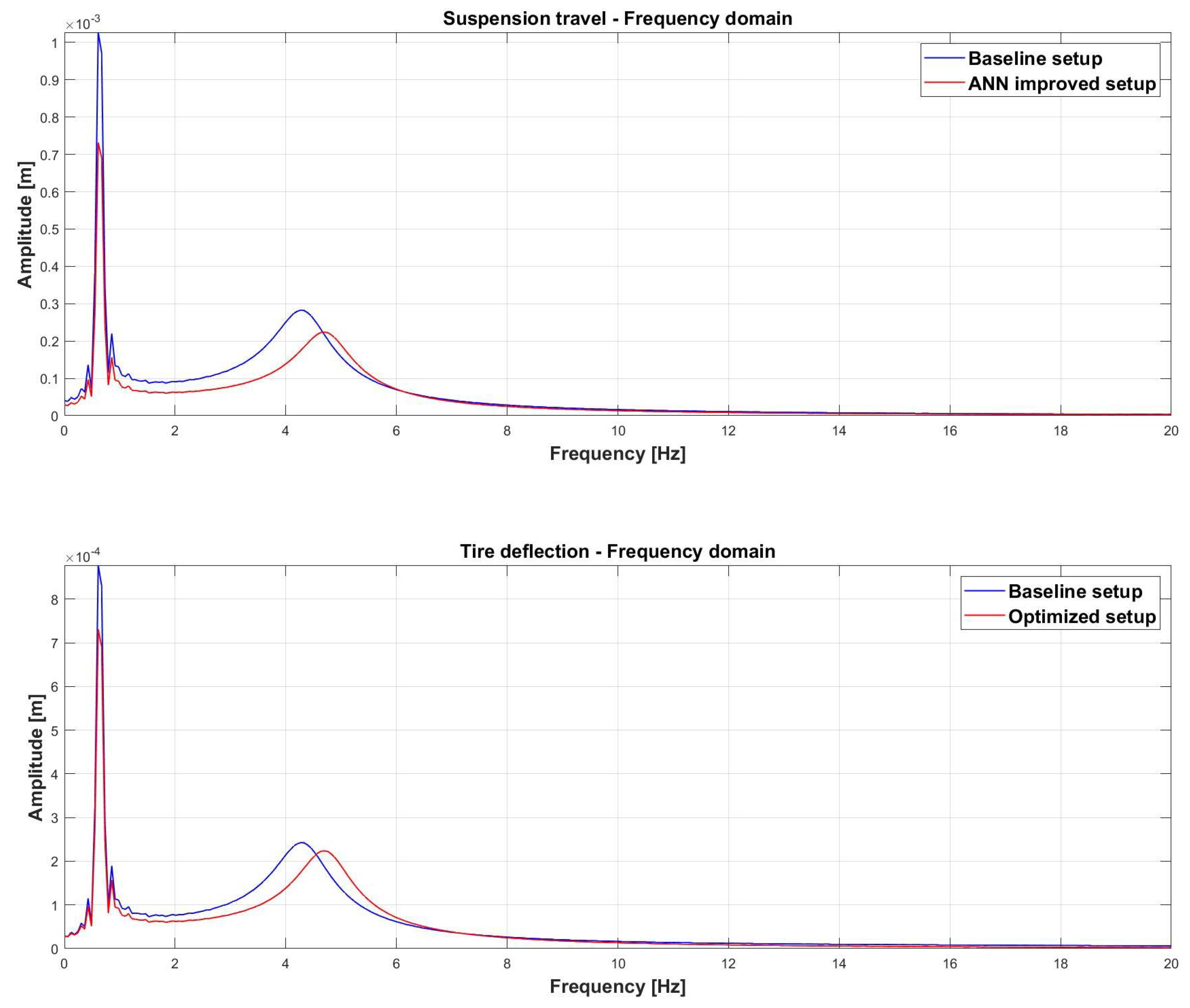
Figure 18.
Comparison between the baseline setup and optimized setup. The optimized setup is able to reduce the resonance peak amplitude of suspension travel and tire deflection in the frequency domain.
Figure 18.
Comparison between the baseline setup and optimized setup. The optimized setup is able to reduce the resonance peak amplitude of suspension travel and tire deflection in the frequency domain.
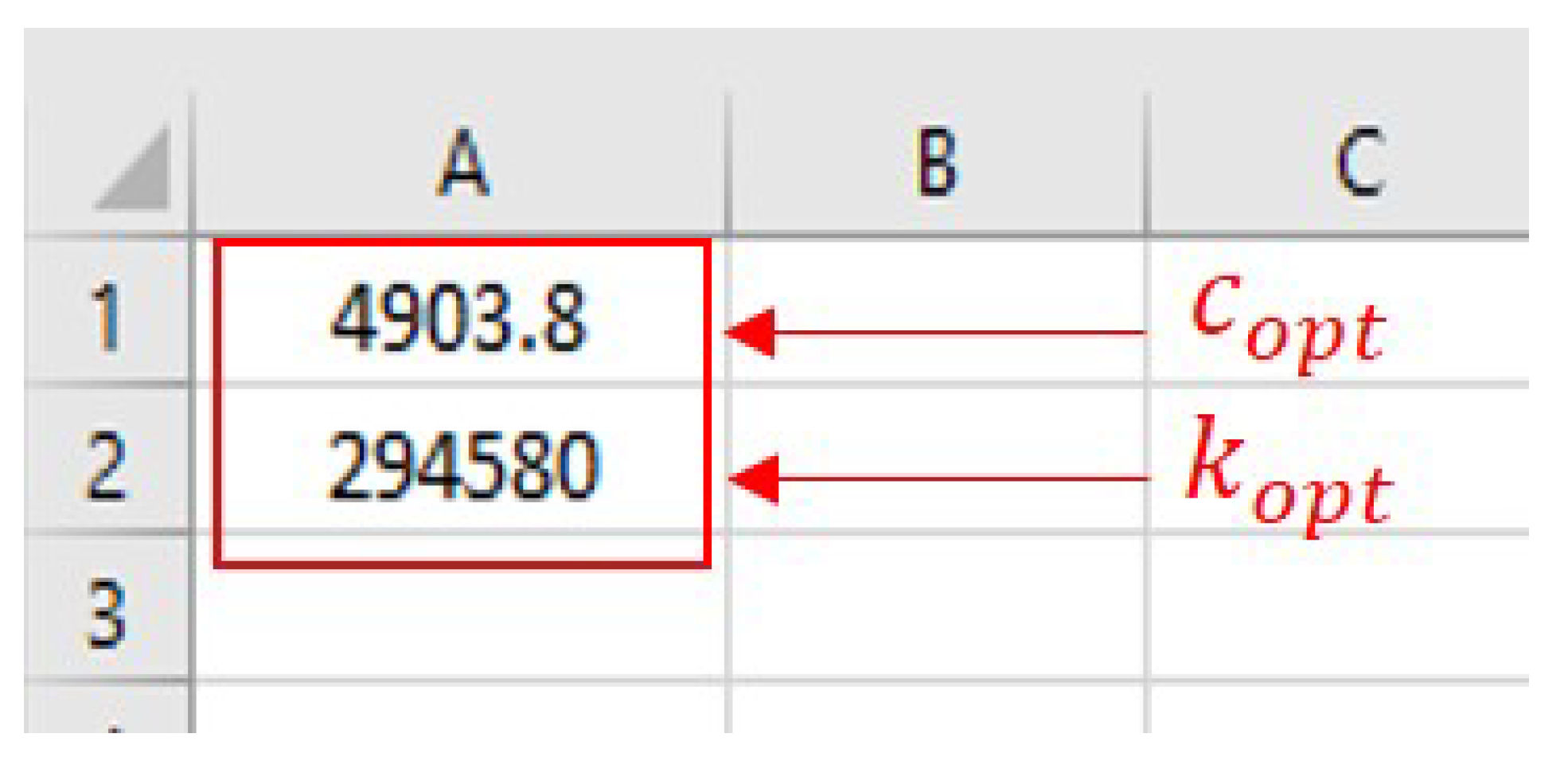
Figure 19.
Output vector of the neural network.
Figure 19.
Output vector of the neural network.
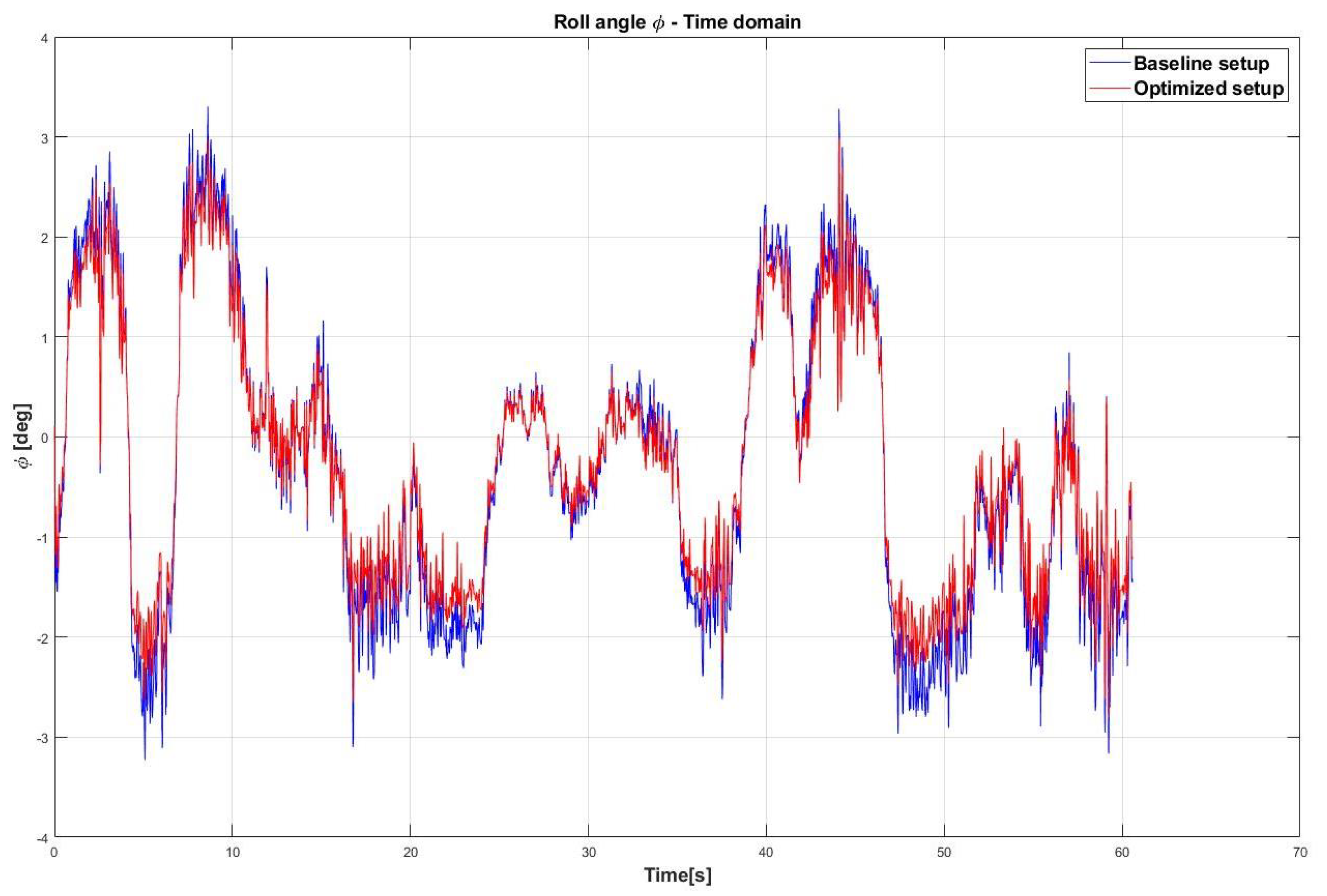
Figure 20.
Comparison between the baseline provided setup and improved setup for the roll angle trend in the time domain.
Figure 20.
Comparison between the baseline provided setup and improved setup for the roll angle trend in the time domain.
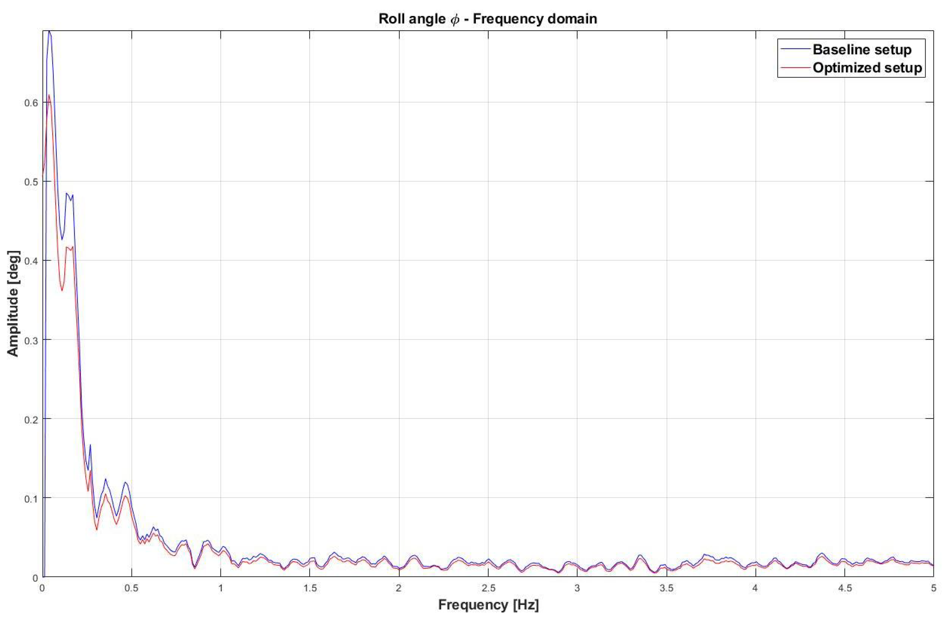
Figure 21.
Comparison between the baseline provided setup and improved setup for the roll angle trend in the frequency domain.
Figure 21.
Comparison between the baseline provided setup and improved setup for the roll angle trend in the frequency domain.
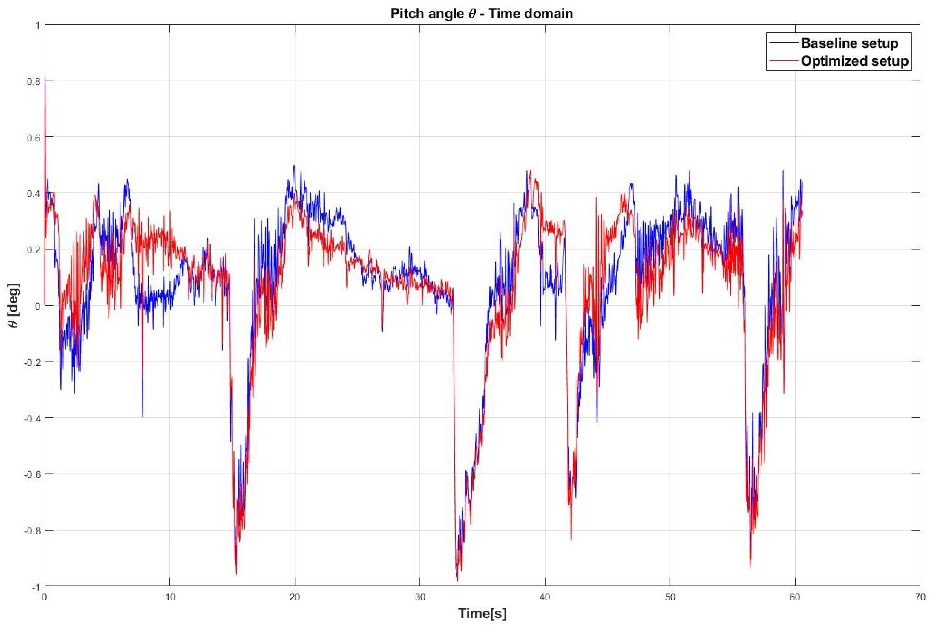
Figure 22.
Comparison between the baseline provided setup and improved setup for the pitch angle trend in the time domain.
Figure 22.
Comparison between the baseline provided setup and improved setup for the pitch angle trend in the time domain.
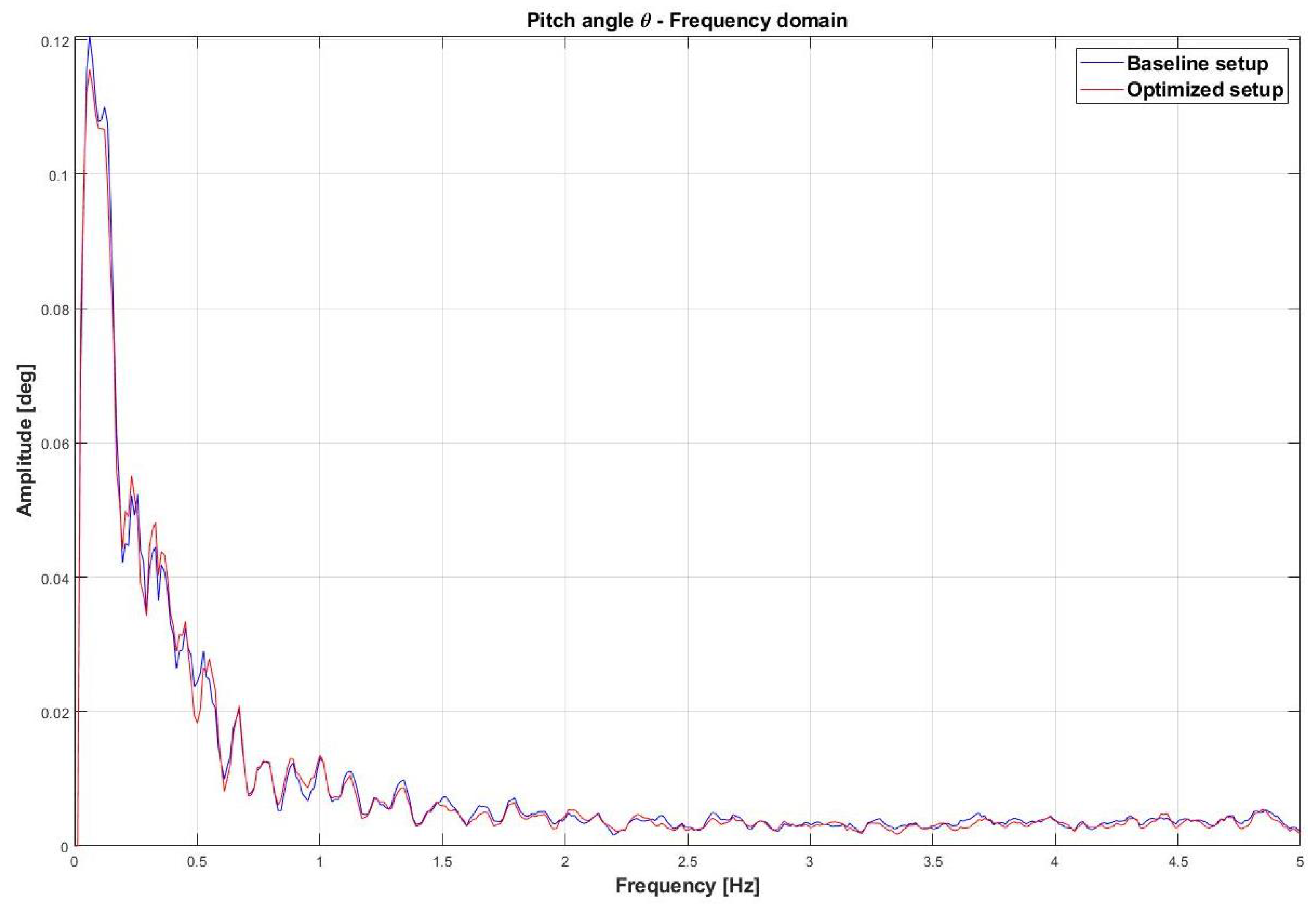
Figure 23.
Comparison between the baseline provided setup and improved setup for the pitch angle trend in the frequency domain.
Figure 23.
Comparison between the baseline provided setup and improved setup for the pitch angle trend in the frequency domain.
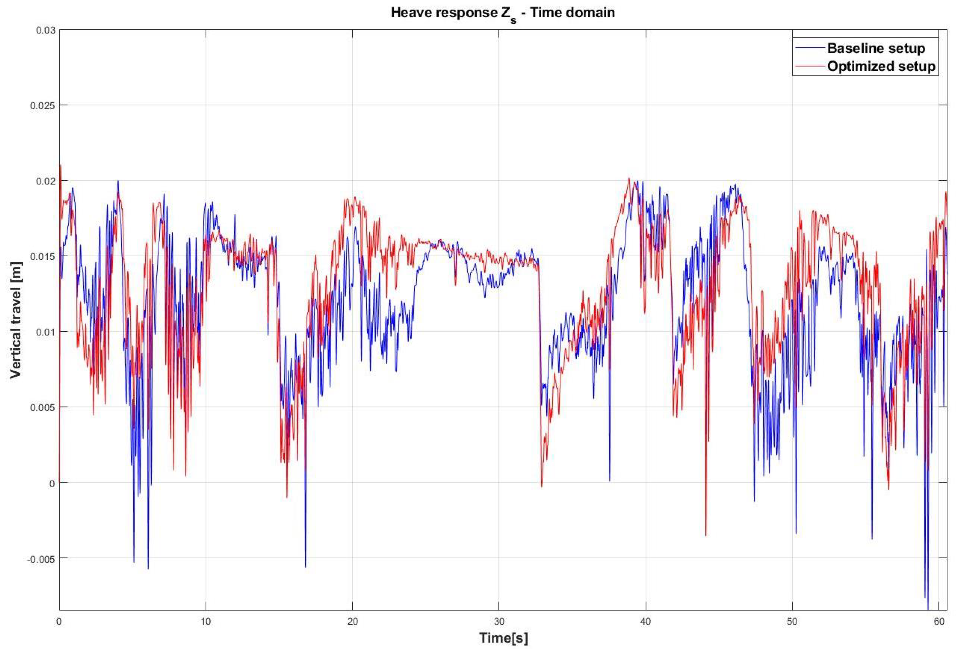
Figure 24.
Comparison between the baseline provided setup and improved setup for heave response of the car in the time domain.
Figure 24.
Comparison between the baseline provided setup and improved setup for heave response of the car in the time domain.
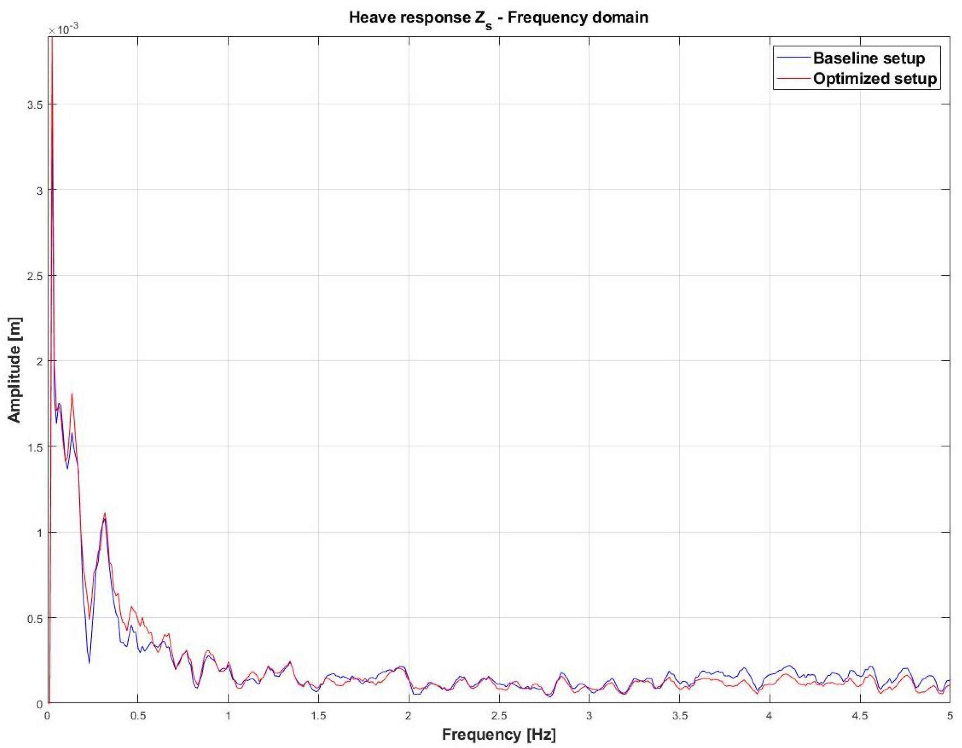
Figure 25.
Comparison between the baseline provided setup and improved setup for the heave response of the car in the frequency domain.
Figure 25.
Comparison between the baseline provided setup and improved setup for the heave response of the car in the frequency domain.
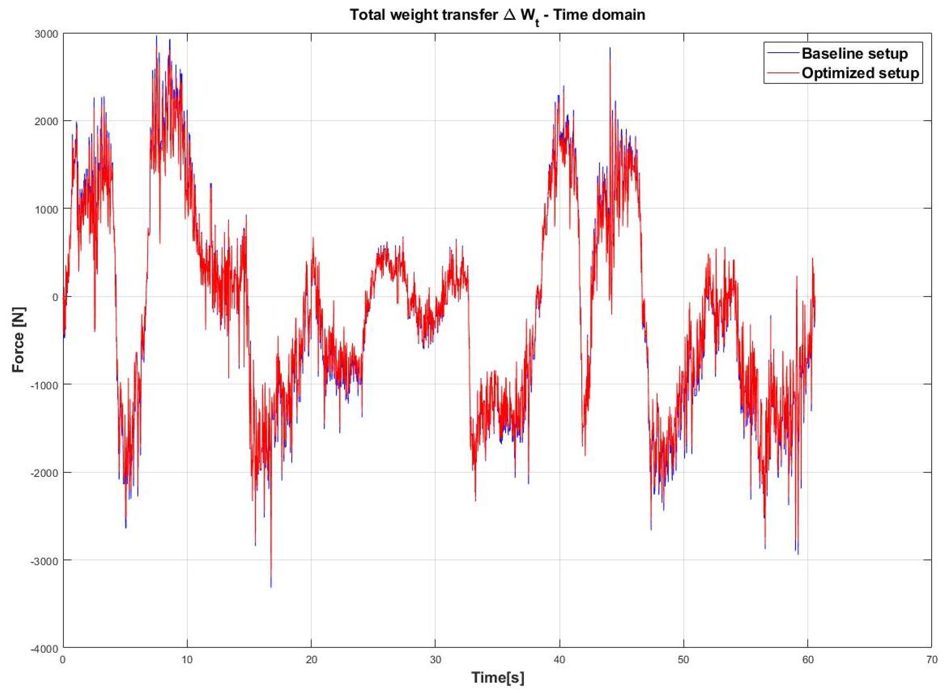
Figure 26.
Comparison between the baseline provided setup and improved setup for the total weight transfer of the car in the time domain.
Figure 26.
Comparison between the baseline provided setup and improved setup for the total weight transfer of the car in the time domain.
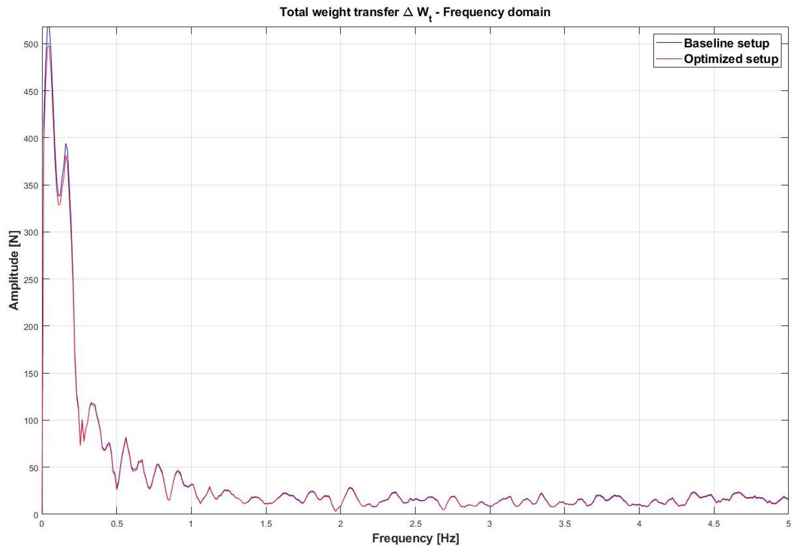
Figure 27.
Comparison between the baseline provided setup and improved setup for the total weight transfer of the car in the frequency domain.
Figure 27.
Comparison between the baseline provided setup and improved setup for the total weight transfer of the car in the frequency domain.
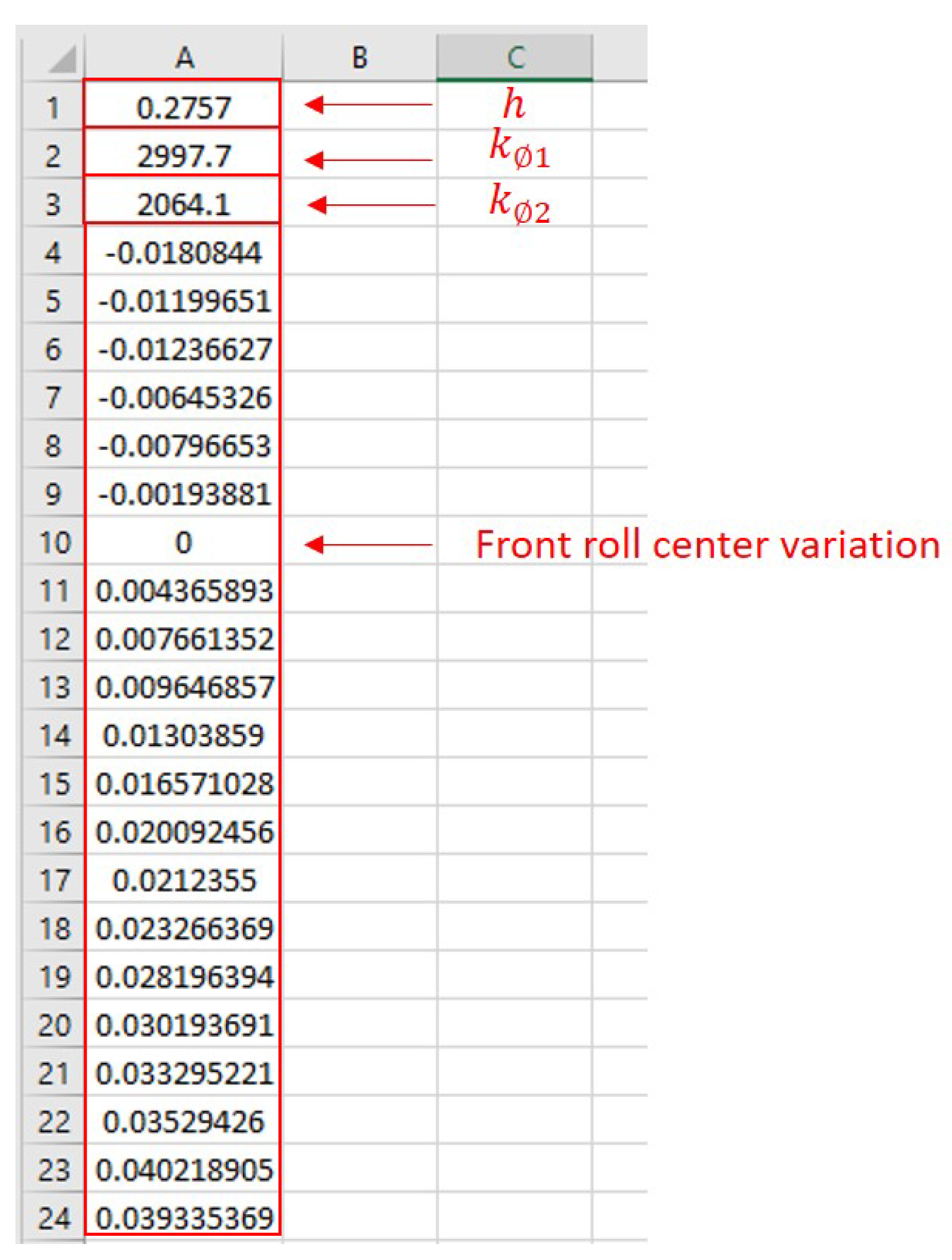
Figure 28.
Output vector of the neural network.
Figure 28.
Output vector of the neural network.
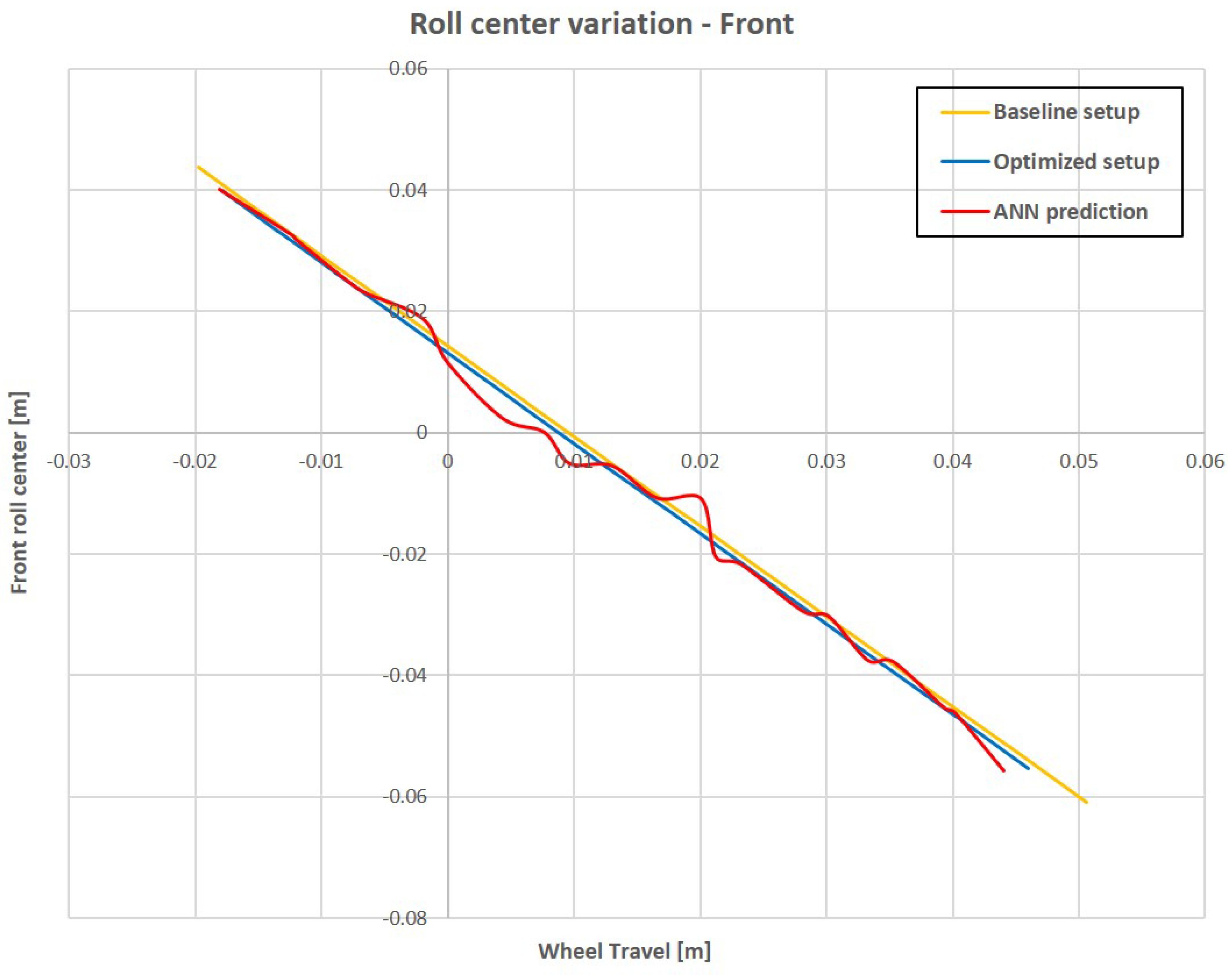
Figure 29.
Front roll center variation comparison.
Figure 29.
Front roll center variation comparison.
Figure 30.
Rear roll center variation comparison.
Figure 30.
Rear roll center variation comparison.
Figure 31.
Front spring characteristic comparison.
Figure 31.
Front spring characteristic comparison.
Figure 32.
Rear spring characteristic comparison.
Figure 32.
Rear spring characteristic comparison.
Figure 33.
Front damper characteristic comparison.
Figure 33.
Front damper characteristic comparison.
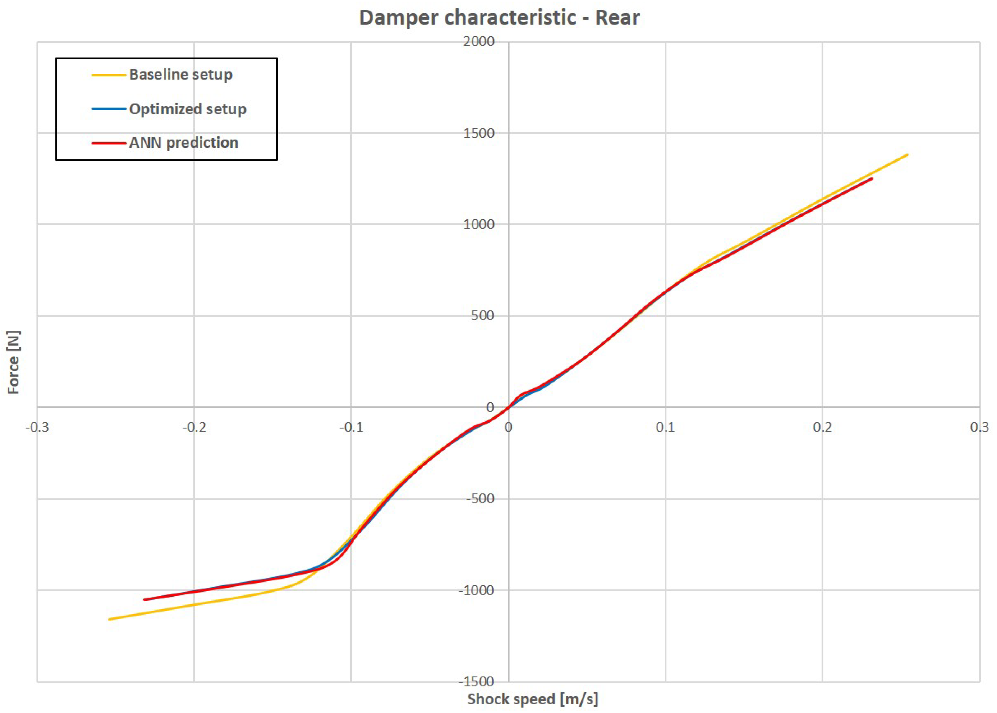
Figure 34.
Rear damper characteristic comparison.
Figure 34.
Rear damper characteristic comparison.
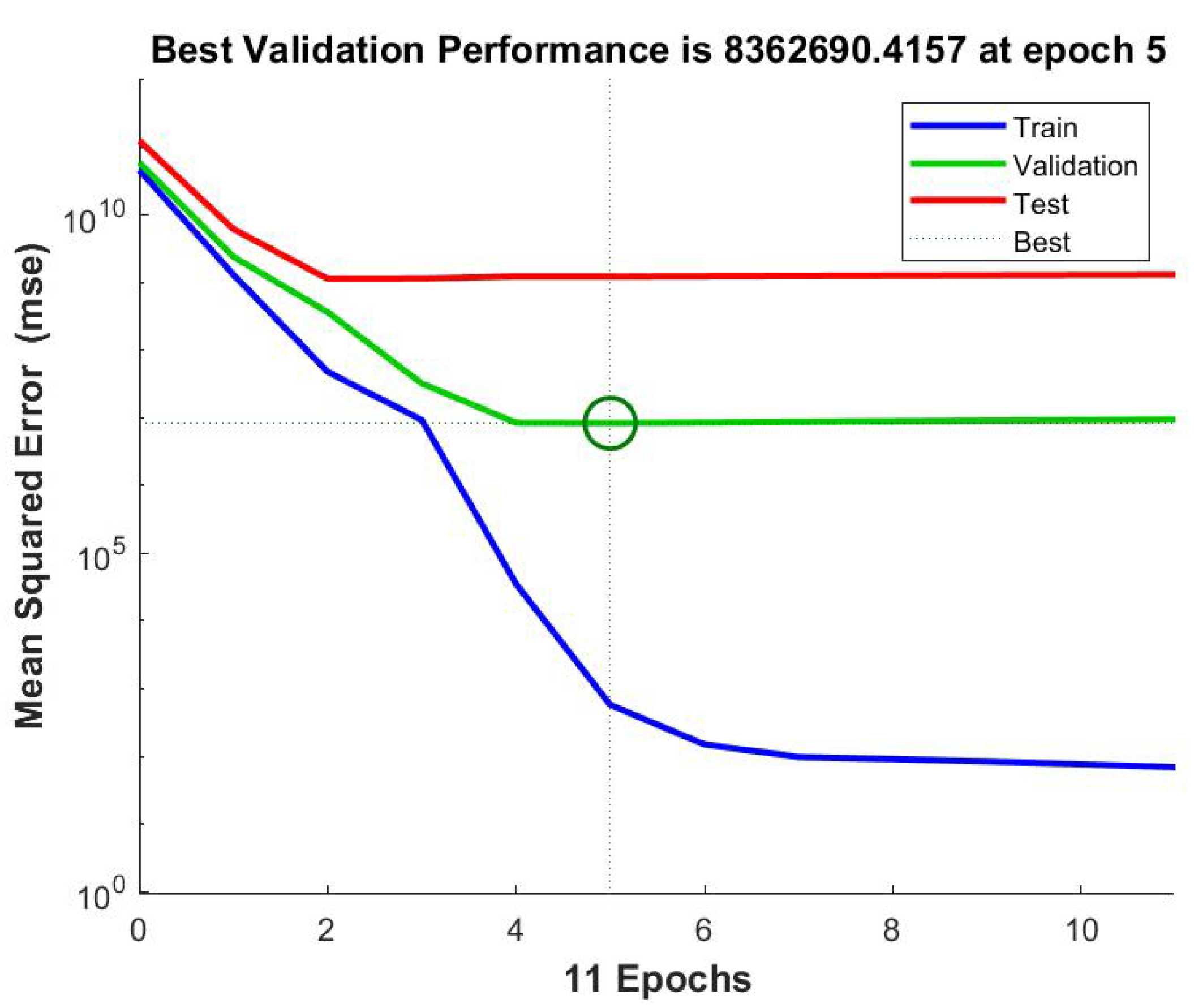
Figure 35.
Correlation coefficient R between target data and output data for training, validation and test and mean squared error for the best validation performance.
Figure 35.
Correlation coefficient R between target data and output data for training, validation and test and mean squared error for the best validation performance.
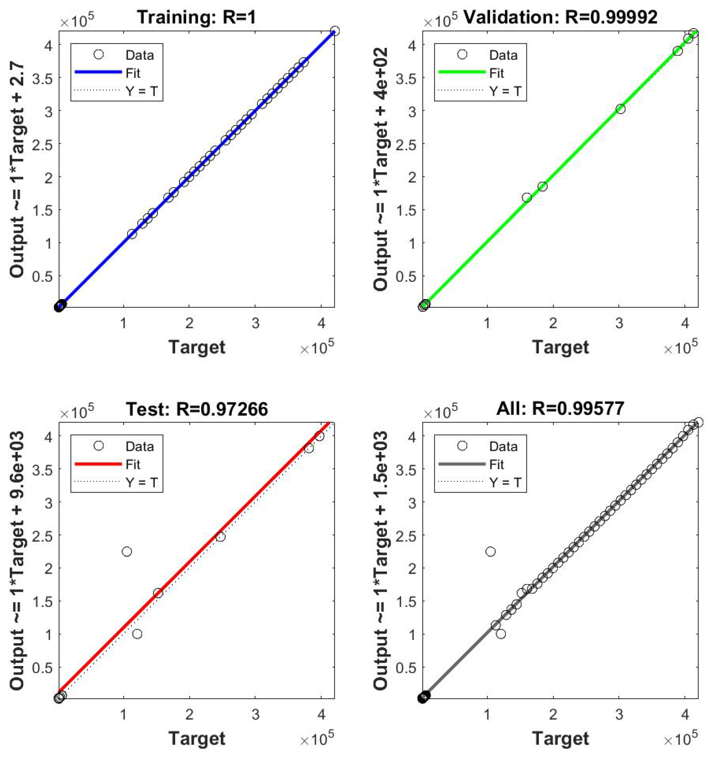
Figure 36.
Correlation coefficient R between target data and output data for training, validation and test and mean squared error for the best validation performance.
Figure 36.
Correlation coefficient R between target data and output data for training, validation and test and mean squared error for the best validation performance.
Table 1.
IndyCar parameters.
Table 1.
IndyCar parameters.
| Variable | Value |
|---|
| Wheelbase l | 3.084 m |
| Front wheelbase | 1.8 m |
| Rear wheelbase | 1.248 m |
| Front track width | 1.7 m |
| Rear track width | 1.58 m |
| Center of gravity height h | 0.30 m |
| Pitch center height b | 0.15 m |
| Vehicle mass m | 673.44 kg |
| Front tire mass | 29.4 kg |
| Rear tire mass | 33.7 kg |
| x-axis inertia | 120 kgm |
| y-axis inertia | 854.34 kgm |
| Front tire stiffness | 294,737 N/m |
| Rear tire stiffness | 276,174 N/m |
| Tire damping | 2000 Ns/m |
| Front dynamic tire radius | 0.66 m |
| Rear dynamic tire radius | 0.7 m |
| Front anti-roll bar ground stiffness | 24,525 N/m |
| Rear anti-roll bar ground stiffness | 26,487 N/m |
| Front roll stiffness | 3297.5 Nm/deg |
| Rear roll stiffness | 2270.5 Nm/deg |
| Front damper motion ratio | 0.994 |
| Rear damper motion ratio | 1.298 |
| Front spring motion ratio | 0.8 |
| Rear spring motion ratio | 0.9 |
| Front anti-roll bar motion ratio | 1.70 |
| Rear anti-roll bar motion ratio | 1.70 |
Table 2.
Parameters chosen for the baseline setup.
Table 2.
Parameters chosen for the baseline setup.
| Variable | Value |
|---|
| Center of gravity height h | 0.30 m |
| Front roll stiffness | 3297.5 Nm/deg |
| Rear roll stiffness | 2270.5 Nm/deg |
Table 3.
Output of the 7-DOF model.
Table 3.
Output of the 7-DOF model.
| Variable | Unit |
|---|
| Roll angle | deg |
| Pitch angle | deg |
| Sprung mass vertical travel | m |
| Front left wheel/road contact point displacement | m |
| Front right wheel/road contact point displacement | m |
| Rear left wheel/road contact point displacement | m |
| Rear right wheel/road contact point displacement | m |
Table 4.
Comparison between the baseline, optimized and predicted ANN setup.
Table 4.
Comparison between the baseline, optimized and predicted ANN setup.
| Parameter | Baseline Setup | Optimized Setup | Predicted ANN Setup |
|---|
| k | 210,412.92 N/m | 294,580 N/m | 294,580 N/m |
| c | 3503 Ns/m | 4904 Ns/m | 4903.8 Ns/m |
Table 5.
Comparison between the baseline, optimized and predicted ANN setup.
Table 5.
Comparison between the baseline, optimized and predicted ANN setup.
| Parameter | Baseline Setup | Optimized Setup | Predicted ANN Setup |
|---|
| h | 0.3 m | 0.2727 m | 0.2757 N/m |
| 3297.5 Nm/deg roll | 2997.7 Nm/deg roll | 2997.7 Nm/deg roll |
| 2270.5 Nm/deg roll | 2064.1 Nm/deg roll | 2064.1 Nm/deg roll |


 ,
, 


