Case Report

Using a Genetic Algorithm with a Mathematical Programming Solver to Optimize a Real Water Distribution System

by
Beatriz Martínez-Bahena
1,
Marco Antonio Cruz-Chávez
1,*,
Erika Yesenia Ávila-Melgar
1,
Martín H. Cruz-Rosales
2 and
Rafael Rivera-Lopez
3
1
Research Center in Engineering and Applied Sciences, Autonomous University of Morelos State (UAEM), Avenida Universidad 1001 Colonia Chamilpa, C.P. 62209 Cuernavaca, Morelos, Mexico
2
Faculty of Accounting, Administration & Informatics, UAEM, Avenida Universidad 1001 Colonia Chamilpa, C.P. 62209 Cuernavaca, Morelos, Mexico
3
Technological Institute of Veracruz, Miguel Ángel de Quevedo 2779, Formando Hogar, 91860 Veracruz, Veracruz, Mexico
*
Author to whom correspondence should be addressed.
Submission received: 28 July 2018 / Revised: 12 September 2018 / Accepted: 14 September 2018 / Published: 24 September 2018
(This article belongs to the Section Hydraulics and Hydrodynamics)

Abstract

:
This research proposes a genetic algorithm that provides a solution to the problem of deficient distribution of drinking water via the current hydraulic network in the neighborhood “Fraccionamiento Real Montecasino” (FRM), in Huitzilac, Morelos, Mexico. The proposed solution is the addition of new elements to the FRM network. The new elements include storage tanks, pipes, and pressure-reducing valves. To evaluate the constraint satisfaction model of mass and energy conservation, the hydraulic EPANET solver (HES) is used with an optimization model to minimize the total cost of changes in the network (new pipes, tanks, and valves). A genetic algorithm was used to evaluate the optimization model. The analysis of the results obtained by the genetic algorithm for the FRM network shows that adequate and balanced pressures were obtained by means of small modifications to the existing network, which entailed minimal costs. Simulations were performed for an extended period, which means that the pressure was obtained by simulation with HSE at one-hour intervals, during the algorithm execution, to verify adequate pressure at a specific point in the system, or to make corrections to ensure proper distribution, this with the aim of having a final optimized network design.

1. Introduction

Water distribution networks (WDNs) are among the most important issues facing society. Without water, humans cannot survive. Therefore, it is of great interest to have water distribution networks that satisfy the needs of users and do not cause economic loss. Water distribution networks play an important role in improving the standard of living in a community, public trades, and industries.
Water distribution is a problem that has been addressed from different aspects: design, operation, rehabilitation, and maintenance. To date, most research has been focused on network design but not on network operation. The operation in a water network is an important issue. An appropriate network design contributes to the network performance but it does not guarantee the efficient distribution. The efficient distribution is closely related to the network operation. Nowadays, network operation is very important because it ensures that the users of the network have just the necessary water, avoiding deficiencies, wastages, and water leakages, among others. So, the water distribution problem involves a network that aims to adequately distribute water. The water network contains hydraulic elements such as pipes, pumps, valves, and supply sources (reservoirs or tanks). The pipes allow water to be drawn from the supply sources to the points of consumption (homes, shops, industries, and fire hydrant irrigation). Supply sources are external sources or sinks for a system; they can be wells, rivers, streams, or connections to other systems. Valves enable adequate control of the pressure in a system. Pumps raise the water from the surface or underground sources to treatment plants, storage, or directly to the distribution system [1,2].
According to computational complexity theory, the water distribution design problem is classified as an NP-Complete problem [3]. It is a complex problem because the computational effort grows exponentially as the instance size increases. In order to solve these kinds of problems, it is necessary to use optimization methods related to the classification of the problem’s complexity [4], such as metaheuristics. Metaheuristics are defined as a high-level strategy which is applied to combinatorial problems with the goal of improving the local optimum. This guides the search process and facilitates the discovery of good solutions. These approximation methods are designed for combinatorial optimization problems in polynomial time. Metaheuristics provide a general framework for creating new hybrid algorithms, combining different concepts derived from artificial intelligence, biological evolution, and statistical mechanisms [5].
For more than three decades, optimization methods and models have been implemented to find the optimal design of water distribution networks, with the aim of having an impact on economic improvement, social benefits and reduction in energy consumption [6]. The problem of designing water distribution networks has been studied by several researchers. The first works about water networks considered it as a linear problem [6,7]. Afterwards, in some works, the problem was considered as a non-linear problem [8,9]. Additionally, the problem has been formulated as a multi-objective problem [10,11,12]. In order to solve the problem, different theoretical optimization methods have been proposed. Some of the employed methods to address the water network problem are mathematical programming [13,14,15], evolutionary techniques such as genetic algorithms [16,17,18,19,20,21,22], and ant colony optimization [23]. Other researchers have implemented real models to improve existing networks, with the objective of finding the best location for control valves in order to obtain adequate pressures and avoid water loss due to leakage in the water distribution systems [24,25,26,27,28]. The problem of the water network has been classified in Classic and Modern stages according to its characteristics and methods of solution, as can be seen in more detail [29]. Many methods have been proposed for solving optimization problems and acceptable results have been achieved to solve theoretical instances. For real instances, heuristics, such as evolutionary algorithms, promise good solutions in limited computing time. Evolutionary algorithms represent a broad class of problem-solving methodologies. Genetic algorithms are very popular and one of the most commonly used methods to solve optimization problems. They were initially proposed by Holland [30]. These algorithms are based on the way in which species evolve and adapt to their environment for survival, according to the principle of natural selection proposed by Charles Darwin [31]. Many of the presented methods to address the water distribution design problem have solved it successfully. However, it is important to mention that, in most cases, the water problem has only been solved for theoretical benchmarks.
This work presents a genetic algorithm that provides a solution to correct the deficiency in the real drinking water distribution network called “Fraccionamiento Real Montecasino” (FRM, Figure 1). This network is located in Huitzilac, Morelos. The hydraulic network is installed at 2250 m above sea level. FRM is a looped network. It has 364 pipes, 350 nodes, 6 tanks, and 1 reservoir. In this network, there are no valves to adequately control the pressure. Gravity is used to supply water to consumers. The FRM network was created approximately twenty years ago. Initially, the network satisfied the hydric user requirements. Through time, due to population growth, more users have been added to the network. Currently, the design of the network is considered inappropriate because most of the users do not receive an acceptable supply service and they have to obtain this indispensable service through other methods. To solve the problem, the addition of new elements to the FRM network is proposed. These elements are storage tanks, new pipelines and pressure-reducing valves. In order to evaluate the hydraulic constraints, one of the best known hydraulic water distribution modeling toolkits, commonly accepted in the scientific community, is used: EPANET solver [1]. Although there are different commercial software and free-ware available on the market for designing and optimizing a variety of water distribution networks [32,33], they are generally used for specific benchmarks, and most of them are theoretical. In previous works, [29,30,31,32,33,34], real networks have been solved by using evolutionary algorithms and EPANET solver, with excellent results. These networks were not modified by adding elements but they were redesigned by modifying the existing network components. In this work, the novel algorithm finds the best solution for the FRM real network instance (which has a previously defined design) by adding new elements with the lowest possible cost to obtain good performance of the network.
Hybridization of the genetic algorithm was performed with EPANET solver. So, the genetic algorithm, here designed, interacts with EPANET solver to evaluate hydraulic constraints. EPANET solver has been employed in a great number of works worldwide [1]. It can be said that the genetic algorithm, here proposed, is a tool used to evaluate the optimization model, which minimizes the cost of new elements added to the system. The viability of a solution obtained by the genetic algorithm is validated by EPANET solver.
Simulations are performed by EPANET for the best solutions obtained by the genetic algorithm. The simulations were performed for an extended period, which means changes to the status of control elements (on/off) and pipes (open/closed) can be made, based on the pressure or water levels at sensing nodes. Therefore, pressure nodes of the network were obtained by simulation with the Hydraulic EPANET Solver in the FRM, at the beginning and during the execution of the algorithm, at one-hour intervals to verify adequate pressure at a specific point in the system or to make corrections to ensure proper distribution.
The present work is organized as follows. Section 2 provides an explanation of the water distribution problem. Section 3 describes the solution methodology proposed in this work: an optimization model, a constraint satisfaction model, and a genetic algorithm. Section 4 shows the obtained experimental results based on the FRM water distribution network. Finally, in Section 5, the conclusions are explained.

2. Water Distribution Problem (Case Study)

The water distribution problem can be represented by graph theory. A graph is denoted as G = ( V , A ) , where V is a set of vertices or nodes and A is a set of edges or arcs. There are different types of graphs. Non-directed graphs have two directions, and directed graphs have only one direction [36]. Figure 1 shows the graph of the FRM network, which is a directed graph because the water flows in one direction. In this graph, the nodes represent supply sources (reservoirs, tanks) or points of consumption (homes, shops, industries, etc.). They are represented by different symbols depending on whether nodes are sources or points of consumption (Table 1). The edges represent the connecting elements such as pipes, valves, and pumps. Each edge has an associated cost which can be the cost of the pipe diameter, the flow velocity in the pipes, the length of a pipe, the cost of the valve, the cost of the pump or another parameter. This representation is important because it is exactly the input parameter that EPANET solver needs to find the hydraulic characteristics of the network, such as pressures, and velocities, among others.
Table 1 shows the symbolic representation of the elements in a network. Some symbols are presented in the original FRM network (Figure 1), such as tanks, reservoirs, consumption points, and pipes. Pumps and valves are not represented in the graph because they do not exist in the current FRM network.
Table 2 summarizes the main elements of the FRM network. There are 364 pipes with a diameter of 22.7 to 101.6 mm. The minimum pressure requirement is 10 mca (meters for water column) and the maximum pressure requirement is 60 mca. The standard demand (pro-capita amount) is the amount of water needed for each node of the FRM network.
To analyze the FRM network, a hydraulic simulation was performed by using EPANET solver. EPANET is a free software that facilitates the analysis of hydraulic behavior in water distribution systems. It was developed by the Environmental Protection Agency (EPA) [1]. It is a tool that can be used in both Windows and Linux environments. It has been used by several researchers [25,26,27,28,29,37], who have worked with water distribution network problems. EPANET calculates the friction loss in pipes using the formulas introduced by Darcy–Weisbach, Manning, and Hazen–Williams [1]. It allows the user to simulate systems of any size. The Hazen–Williams formula is more commonly used for water flows while the Darcy–Weisbach formula is more commonly used for other liquids. So, in this work, the Hazen–Williams formula was used. The roughness coefficient value is set as 125 because the pipes are made of galvanized iron. Additionally, it can be used for new or used pipes [38]. Finally, this parameter was set with this value based on the observation that the results of the optimization model were affected by it. This meant pressure and velocities were lower when this value increased. EPANET tracks the flow rate for each pipe, the pressure at each node, and the water level in the tanks over a period of time. Figure 2 presents the pressures obtained at each node over a period of 72 h. The results show that there are several nodes with pressures that do not reach the minimum pressure requirements. A total of approximately 24 nodes have negative pressure, which indicates that water does not reach the nodes. Even when negative pressures are hydraulically impossible, EPANET mathematically obtains them and gives them as a result of an inappropriate performance of the network, due to it having the lowest or no pressures. At the other extreme, excess pressure could lead to problems of pipe ruptures, thus leading to water leaks and economic loss [35]. This was the first test, and it was carried out by using the initial design of the FRM instance, previously described.
In order to find a solution (water supply for all users), the existing hydraulic network, FRM, must be redesigned. For this specific network, changing the diameter of the pipes is not a feasible solution because it is too expensive. Additionally, it is important to mention that the objective of this work is to use the same network and make the smallest possible number of changes on it. The rebuilding process would involve excavating buried pipeline throughout the network, which probably means a new redesigned network, with economic and time costs that are higher than the resulting costs of just adding some elements. One solution, here proposed, is adding new storage tanks, and considering new pressure-reducing valves (PRVs), pipes, or pumps. To add the pumps, pipes, or PRVs to the existing hydraulic network, an optimum configuration must be obtained. This new configuration must be generated with the lowest possible cost. An optimization model is proposed, which takes into account the problem representation and the network. The objective of the model is to find the minimum number of necessary additional tanks, valves, and pipes to be added. In order to ensure efficient operation of the hydraulic network, an attempt is made to minimize the cost of the necessary modifications.

3. Solution Methodology

3.1. Optimization Model

In this work, an optimization model is proposed. This model is composed of an objective function and a set of constraints, which allow suitable functioning in a water distribution system.
min   C ( P , T , V ) = T = 1 n T i = 1 n d j = 1 p C i L i j X i j T + T = 1 n T C T Y T + V = 1 n V J = 1 n P C V K V J
Subject to
i = 1 n d j = 1 p X i j T = 1                                     T
d m i n d i j d m a x
X i j T { 0 , 1 }
Y T { 0 , 1 }
K V J { 0 , 1 }
Equation (1) represents the objective function. It attempts to minimize the total cost of the changes made in the network: the cost, C i , of the new pipes, tanks, C T , and valves, C V , where n T is the number of tanks, n d is the number of diameters, p is the number of pipes for the new tanks, n V is the number of valves, and n P is the number of pipes to insert into the new valve. L i j is the length of each pipe j with diameter i . In this work, the costs of new components were calculated based on commercial costs from the year 2015 [39]. Constraint (2) indicates that pipe diameters are on the list of commercial diameters. For each pipe segment, only one diameter is used. Constraint (3) ensures that the chosen diameter is included on the list of available commercial diameters; it indicates that the diameter i of the pipe j , d i j , is greater than the required minimum diameter d m i n and lower than the maximum diameter d m a x . Constraint (4) indicates whether a diameter is being used or not. For example, if X i j T = 1, the diameter is being used. If the diameter is not being used, then X i j T = 0. It should be noted that the network may have repeated diameters. Constraint (5) indicates that a tank is selected if Y T = 1, otherwise Y T = 0. The tanks can have different characteristics such as diameter, initial water level, maximum water level and minimum water level. Constraint (6) indicates whether a valve V is inserted into a pipe J . If a valve is inserted into the pipe, then K V J = 1, otherwise, K V J = 0. The valves can have different characteristics such as valve setting and diameter.

3.2. Constraint Satisfaction Model

A constraint satisfaction model is presented [35], in which a set of hydraulic constraints must be met in order to obtain proper system functioning by satisfying the needs of the users.
i Q i n i Q o u t = Q e
c h f = c E p
H m i n H i H m a x
Equation (7) represents the physical law of mass conservation, where the sum of the flow entering and leaving a node must be equal to zero. The constraint indicates that the flow that enters a node, Q i n , minus the flow that leaves a node, Q o u t , is equivalent to the demand Q e . Equation (8) represents the law of energy conservation. It indicates that the sum of the frictional energy losses h f in any circuit c must be equal to either zero or the power energy, E p , supplied by a pump. Constraint (9) refers to the minimum and maximum pressure requirements that satisfy water users, while guaranteeing appropriate network operation. The constraint necessitates that the pressure at a node H i be greater than the required minimum pressure H m i n and lower than the maximum pressure H m a x . The pressures are defined according to the characteristics of the FRM network problem.

3.3. Solution Strategy

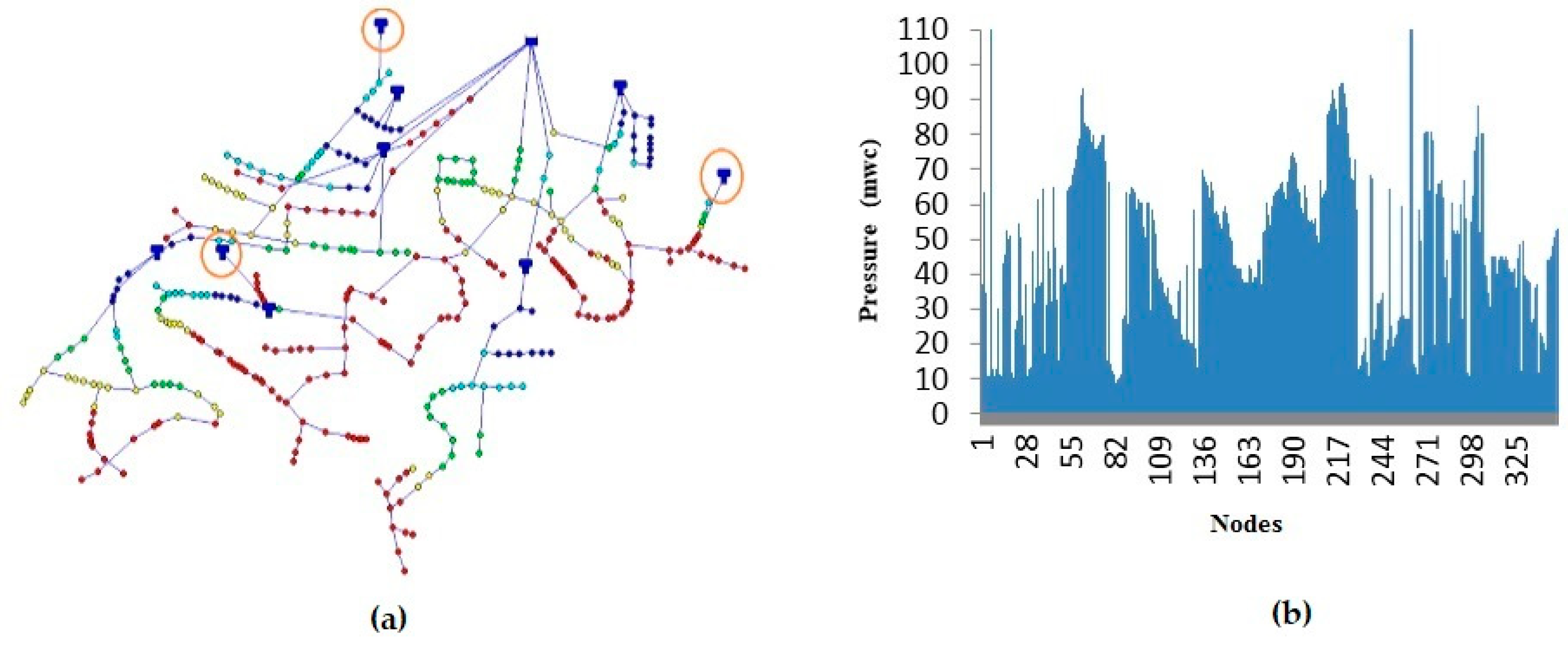
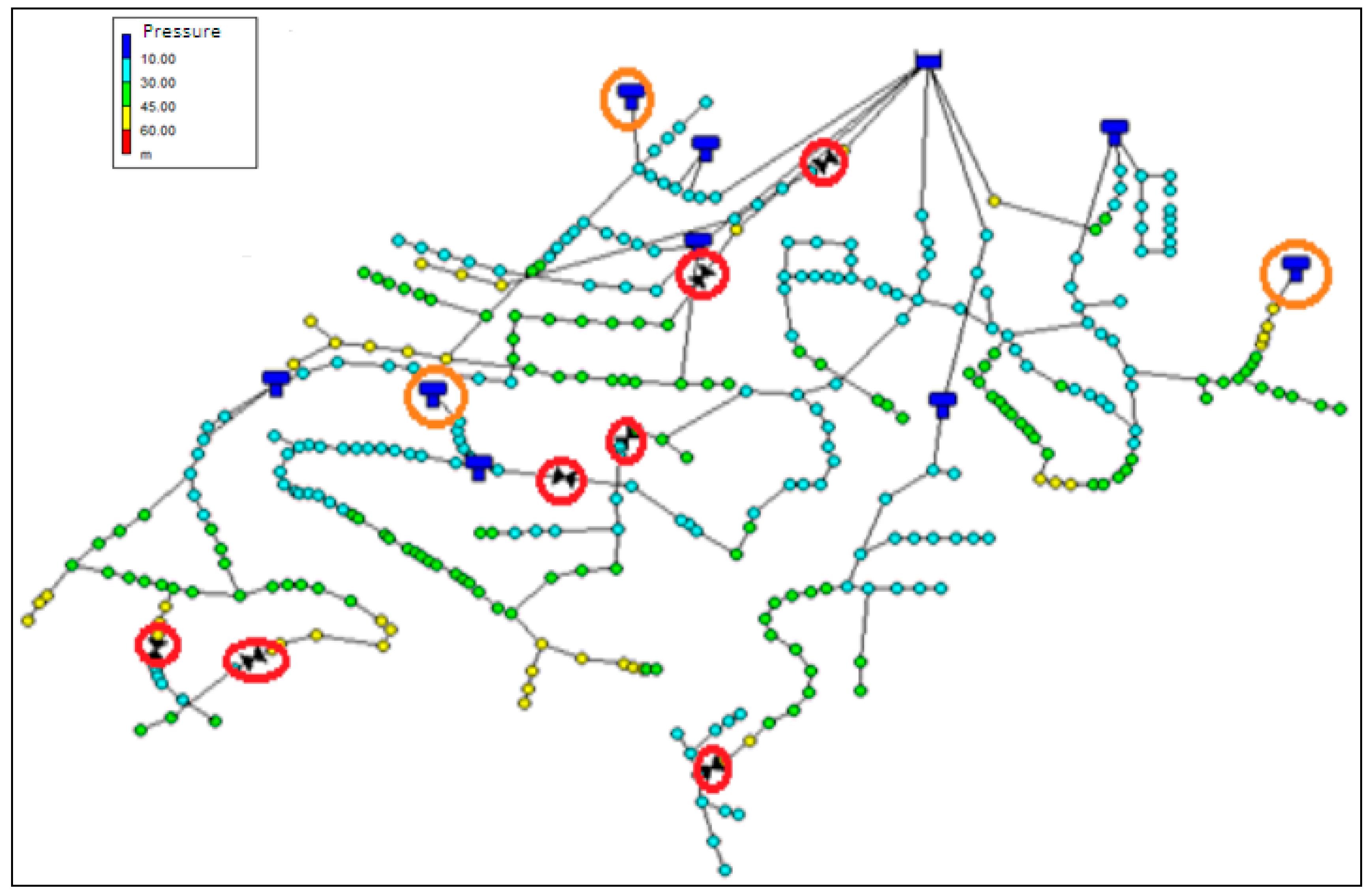
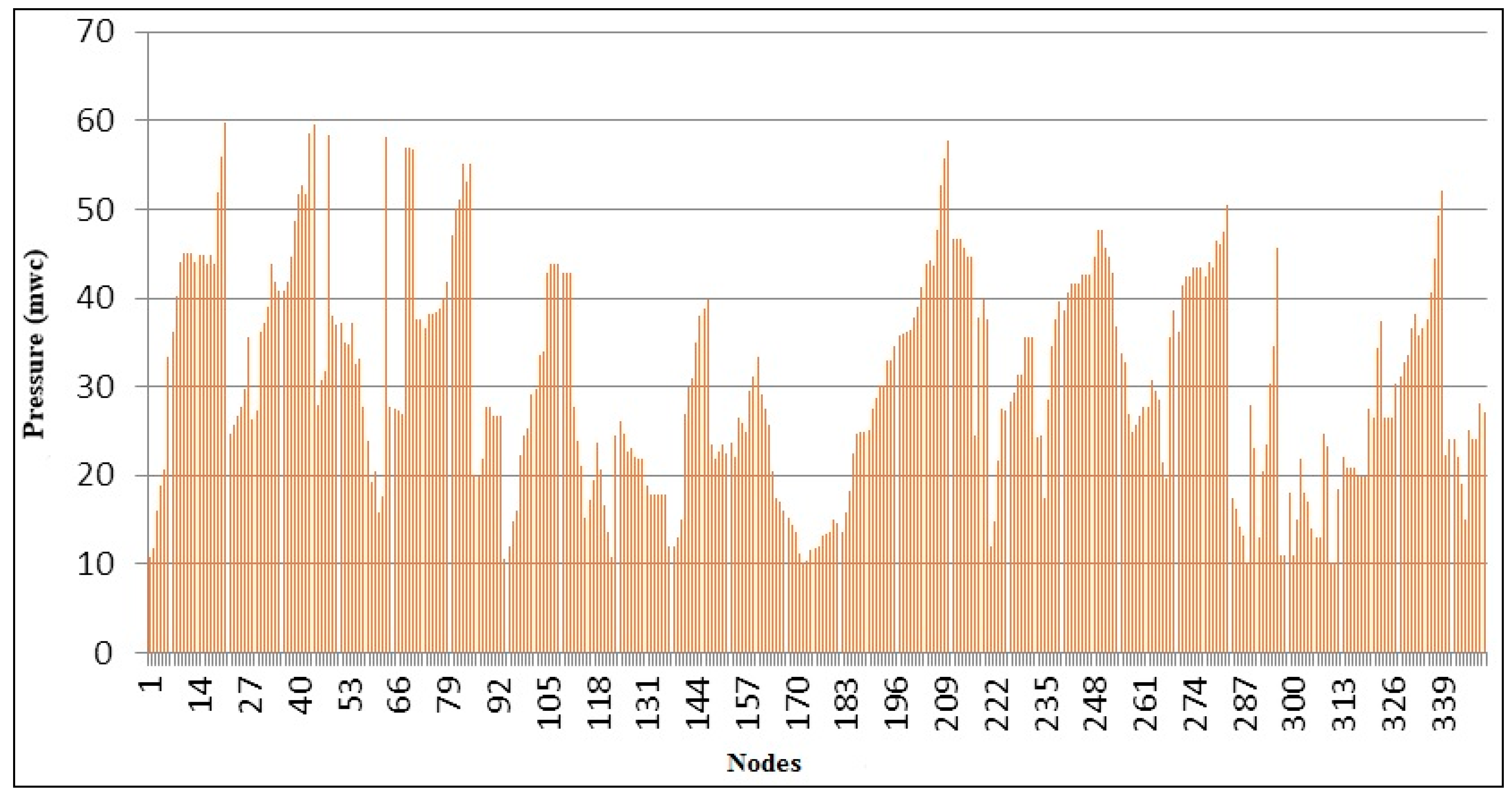
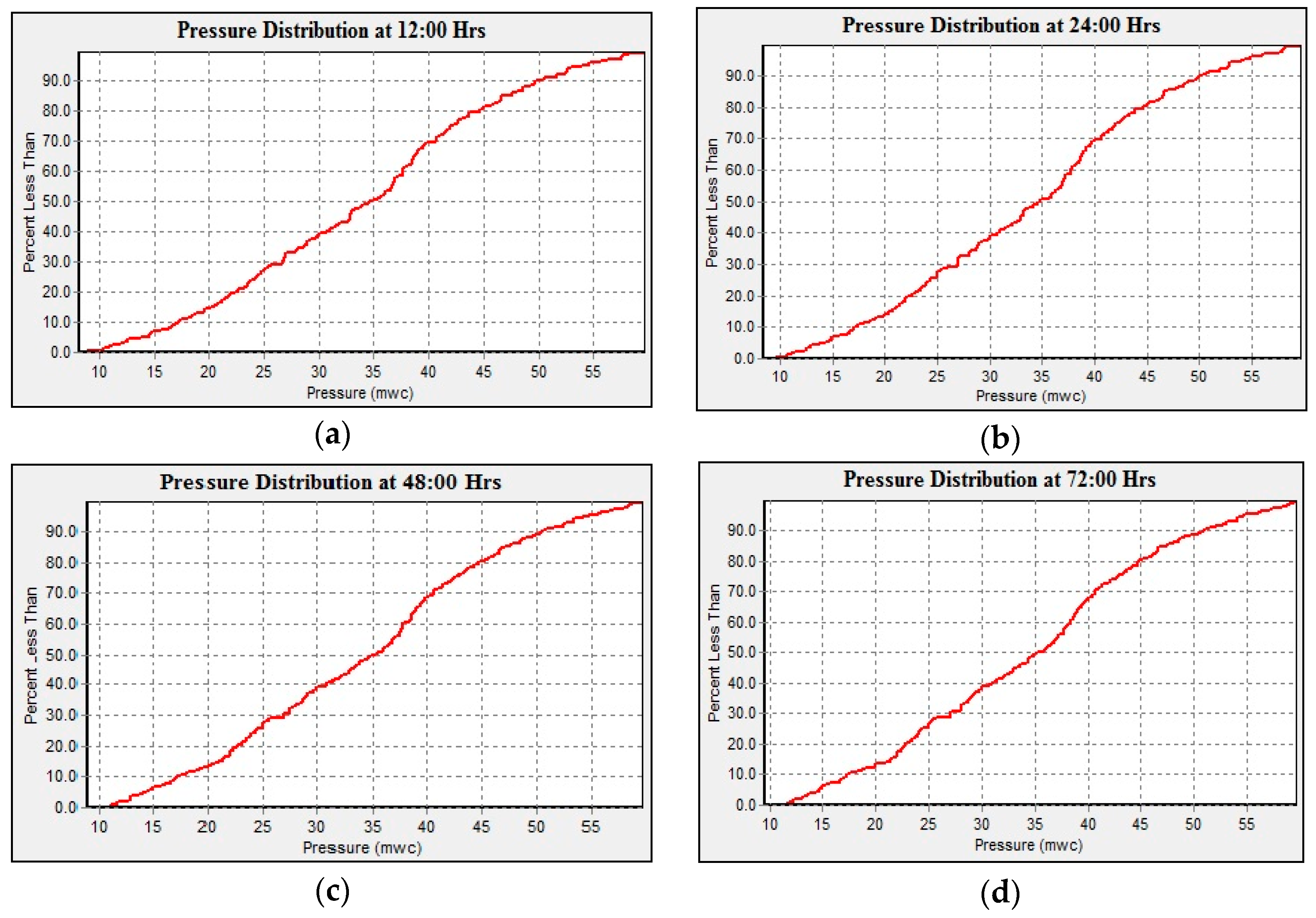
  • Add new storage tanks with appropriate characteristics at points in the network where the minimum pressure is not reached. The benefit of implementing storage tanks with gravity water distribution is that it reduces or eliminates the number of necessary pumps, thus reducing the energy costs. The main purpose of this work is to increase the pressure in the water distribution system. In order to do this, the coordinates of the possible tank locations are determined according to the topography of the network. It would not be possible to add a tank where there is an existing building, or to install a pipe in an area considered risky. The process of choosing the candidate positions for inserting an element (tank, pipe, PRV) includes first checking points where pressure is not reached and then verifying the feasibility of adding the element. For proper system operation, it is necessary to establish the required characteristics for the new storage tanks such as diameter, volume (m3), maximum level, minimum level, and initial level. Figure 3 shows the results obtained from the simulation performed during a 72-h period in EPANET solver. Three storage tanks with different characteristics were added (Figure 3a). Pressure increased at nodes that did not reach the required minimum pressure (Figure 3b). For the solution to be feasible, the maximum pressure requirements must be considered. The graph shows high pressures at several points in the network (red vertices, Figure 3a); therefore, the solution is unfeasible [35].
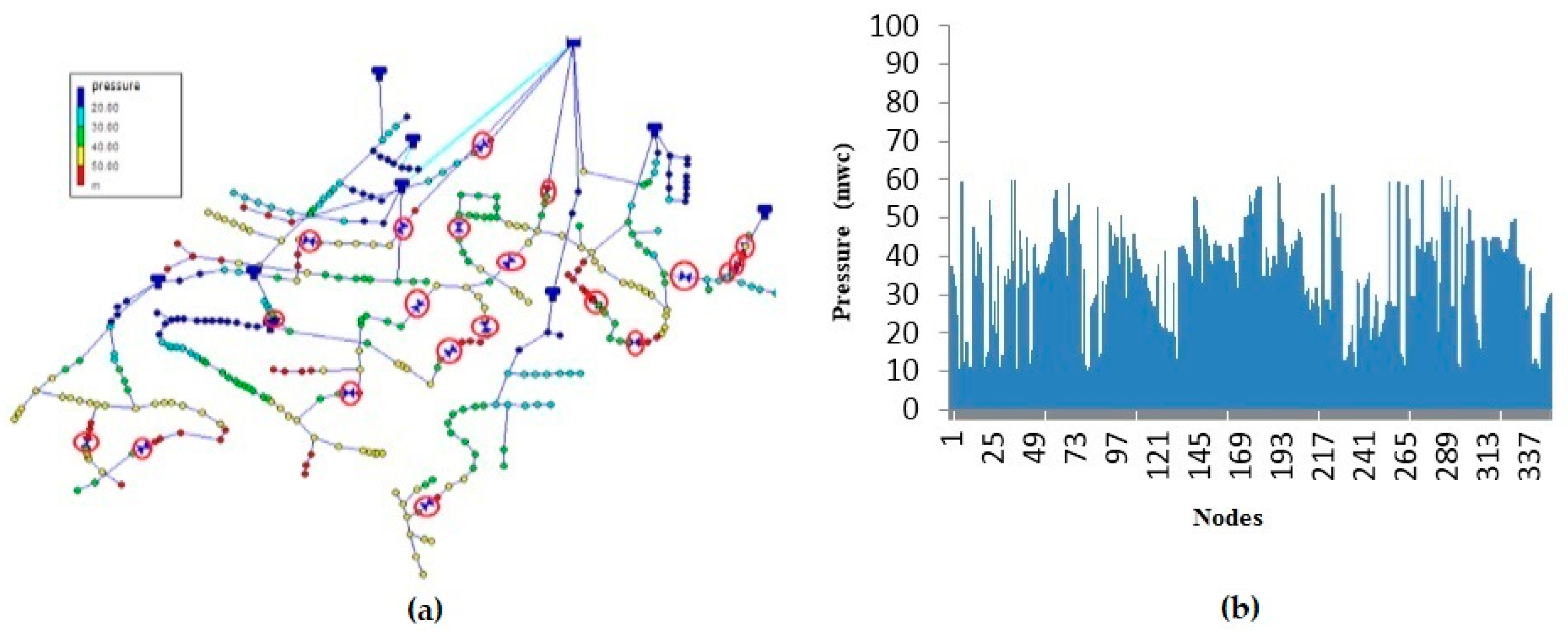
  • Add a pressure-reducing valve (PRV), which allows the pressure to be reduced if it is very high. This ensures balanced service to the community and avoids constant pipe breaks. The problem of finding the optimal valve location in a system has been studied for years by different authors [24,25,26,27,28,40,41] in order to improve water distribution while minimizing operation costs. When a valve is added, an economic cost is generated. As more valves are added to the system, the cost increases. This work adopts the idea of [42], which suggests adding valves only in the pipes that connect nodes with pressures greater than the maximum limit. It is important to mention that each pipe is considered as a candidate for valve insertion. However, inserting a valve into the pipes that connect nodes without high pressure can decrease the pressure too much, or even create negative pressure. The solution would no longer reach the minimum pressure required, and it would therefore be unfeasible. To insert the valves, a few points are considered [43]. The direction of the valve must be the same as the direction of the original water flow in the selected pipe. In addition, the diameter of the valve must be the same as the diameter (22.7–101.6) of the chosen pipe. The pressure setting in the range of 10–60 mca is determined to perform the most realistic simulation possible. Figure 4 shows the results of adding pressure-regulating valves. Twenty-two valves were added (Figure 4a). As a result, the nodes met the maximum pressure requirements (Figure 4b). Therefore, the solution is feasible because it satisfies the constraints of the model.
    The proposed solution strategy obtains feasible solutions according to the constraint satisfaction model. It is also necessary to employ the optimization model in order to reduce the costs of modifications made to the FRM network. In this work, a genetic algorithm is implemented, since good results have been obtained with genetic algorithms in other investigations of water distribution systems [25,26,27,32].

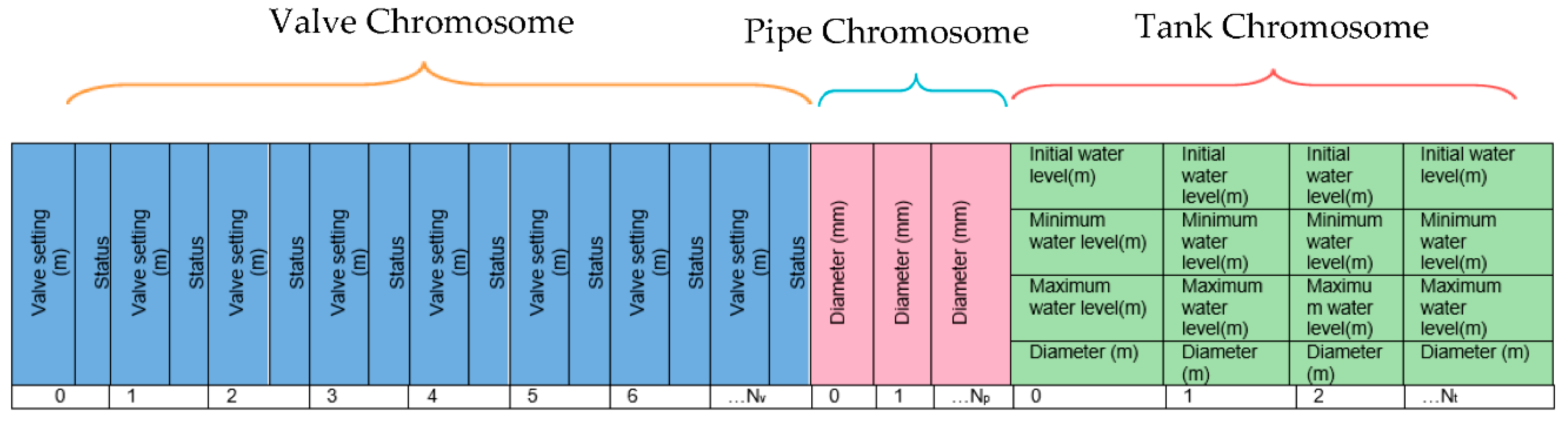
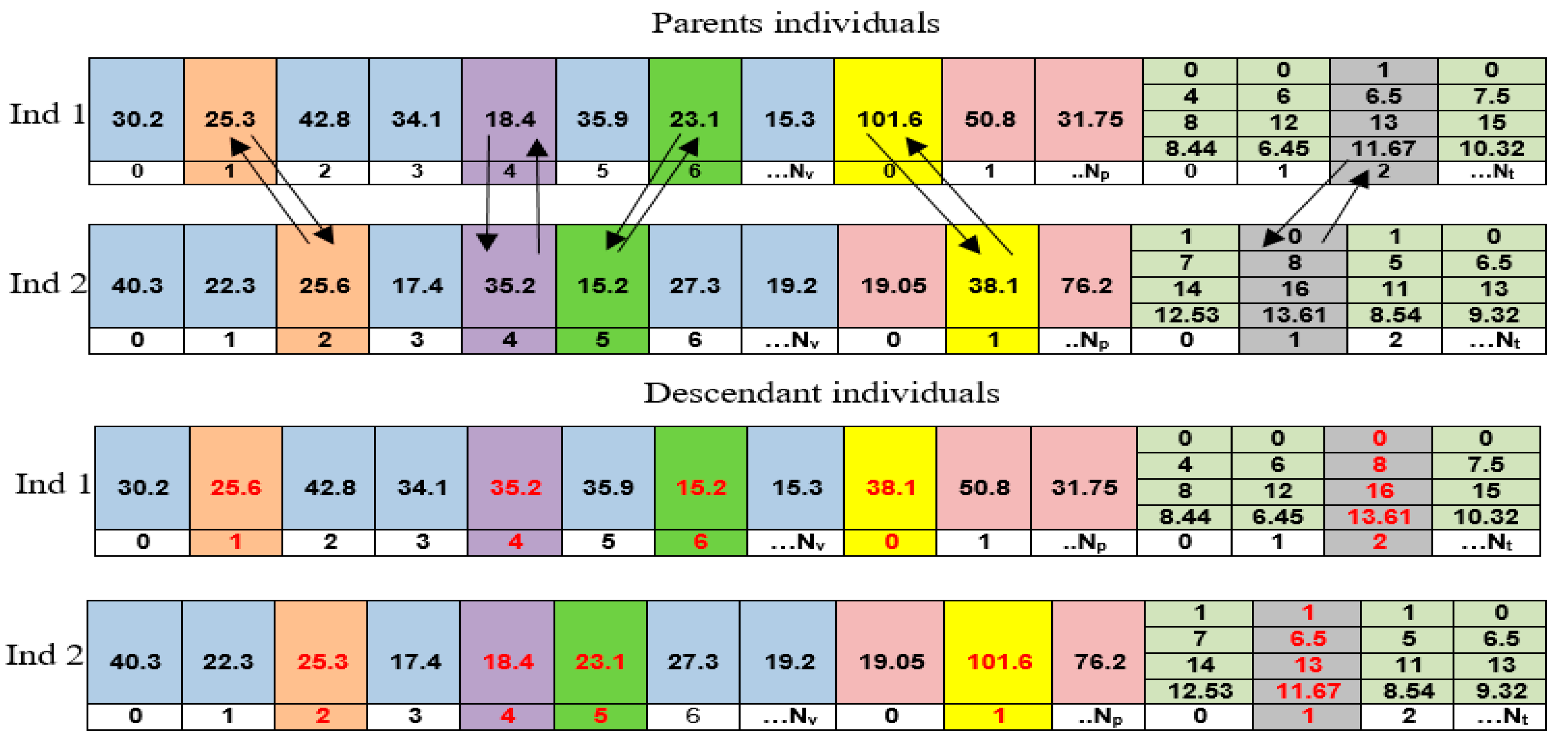
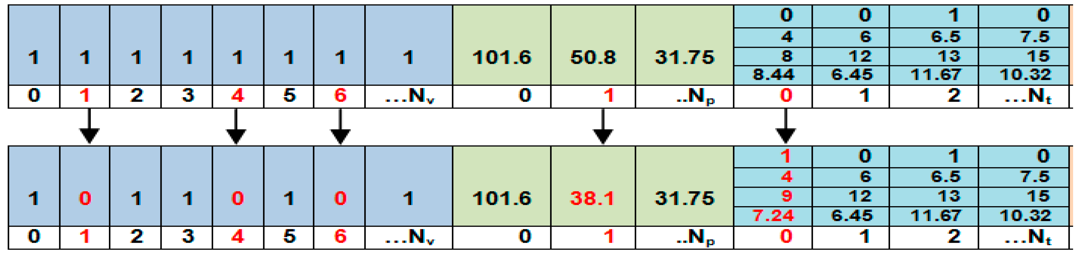
3.4. Genetic Algorithm

Genetic algorithms (GAs) were invented by Holland [30] and introduced by Goldberg [44] as evolutionary type algorithms. GAs are adaptive methods that have been widely used to solve search and optimization problems. These algorithms are based on the genetic process of living organisms. Over generations, populations evolve according to the principles of natural selection and survival of the fittest individual. This theory was proposed by Charles Darwin [31].
Representation of individuals. A solution for the FRM network is represented as an individual, consisting of several chromosomes. A chromosome is a set of genes. A gene represents a value of the solution. The individual, for the FRM network, is coded as a string of binary, real, and real or integer values. Figure 5 shows the graphical representation of an individual. It has three chromosomes (valve, pipe, and tank). The valve chromosome is a gene with two attributes: ‘valve setting’ and ‘status’.
The attribute ‘valve setting’ is defined by the valve closure percentage which is converted to a head loss coefficient. This attribute is set as a real value. The ‘status’ attribute has a binary value. It is used to indicate the existence of a valve in a pipe. Hence, if there were a valve in the pipe, the assigned value would be 1; otherwise, the assigned value would be 0. This value of ‘status’ attribute is assigned based on the information of the existing network. For the FRM individual, this value is 0 because it does not have any valve.
For the pipe chromosome, the value of the gene is the diameter of the pipe and it is taken from a list of eight available commercial diameters, defined prior to the optimization run (12.7, 19.05, 25.4, 31.75, 38.1, 50.8, 78.2, and 101.6, in millimeters). Finally, the tank chromosome is made up of four genes: initial water level ((minimum level + maximum level)/2), minimum water level (1 m), maximum water level (15 m) and diameter. The gene values for each chromosome were coded randomly according to a range of values obtained after an analysis of the parameters of the FRM network.
Feasible initial population. The evaluation of the population is critical because it determines whether an individual has the appropriate characteristics to be part of the population. The feasibility of each individual is determined with respect to the constraint satisfaction model. The model is evaluated by using EPANET solver to verify compliance with the law of conservation of mass at each node, the law of conservation of energy in each circuit, and the necessary pressures at each node for the water distribution system to function correctly. For the FRM network, a feasible solution is considered if each node has a minimum pressure of 10 mca and a maximum pressure of 60 mca.
The crossover operator consists of exchanging the characteristics of two parents to generate two offspring. In this work, a new crossover operator is proposed called genetic interchange between individuals (GIBI). Figure 6 presents an example of the behavior of the GIBI operator. For the valve chromosome, a valve position is chosen randomly. The crossing operation was carried out in the operation configuration through the ‘valve setting’ attribute. The attribute ‘status’ keeps its original value due to valves not moving to another pipe and they are also not removed from the pipes.
Having two individuals, the crossover operation is as follows: for the first individual, the Positions are 1, 4, and 6. Likewise, for the second individual, the Positions are 2, 4, and 5. The gene exchange (valve setting) is performed between {{1, 2}, {4, 4} and {6, 5}}. The process continues until a specified number of exchanges is realized. This specified number is randomly determined as a function of the total number of valves. For the pipeline chromosome, the pipeline position is selected. For example, Position 0 is selected for the first parent, and Position 1 for the second parent. The value of the diameter is exchanged, until a specified number of exchanges has been performed. This number is randomly determined as a function of the total number of pipes. Similarly, for the tank chromosome, a tank position is randomly chosen for each individual. For example, 0 is chosen for the first individual and 1 for the second individual. The genes are exchanged (initial water level, minimum water level, maximum water level, and diameter), until a specific number of exchanges has been performed. The number of exchanges is randomly determined as a function of the total number of tanks.
Mutation operator. The proposed mutation operator makes small random alterations in the genes of a percentage of individuals. Figure 7 shows an example of the mutation operator’s procedure. First, an individual is randomly selected from the population. Then, a position (which corresponds to a valve) on the valve chromosome is randomly chosen. For example, Position 1, 4, or 6 could be chosen, and the value 1 could be changed by 0. This means that the valve would be removed from the pipe, therefore the setting of the valve would not be modified. In other words, it means that a slight alteration is made in the ‘status’ attribute. The values of the valve setting and tank parameters have been defined prior to the optimization run. The pipe chromosome determines the new pipe that connects new tanks with other elements in the network. A position is randomly chosen, for example, Pipe 1. A diameter is also randomly chosen from the list of commercial diameters. In this case, the diameter 50.8 was changed by 38.1. For the tank chromosome, a tank is randomly chosen, for example, tank 0. Its characteristics (initial level, minimum level, maximum level, and diameter) are randomly modified. The ranges of the parameters for the tanks, the diameters of the pipes and the valve setting are input data for the optimization algorithm. These values were obtained according to a field analysis of the FRM network.
Algorithm 1 shows the genetic algorithm. First, the algorithm initializes the input parameters, such as crossover probability ( P c ) , mutation probability ( P m u t ) , population size ( T p o b ) , number of generations ( N g ) , average of selection ( P s ) , and average of mutation ( P m ) . The termination criterion of the algorithm was set as 100 generations. This value was enough to reach an asymptotically low value of the objective function. It meant that the convergence of the algorithm was generally reached before 100th generation, so this value was assigned as the termination criterion, as a result of a tuning process. The instance data is loaded and the initial configuration is created. The values used in the initial configuration depend on the sensitivity analysis that was performed for the input parameters. The algorithm then generates a random initial population of individuals (Line 5). The feasibility of individuals in the population is evaluated using the EPANET functions in Linux platforms [29]. The fitness value is evaluated for each individual (Line 7). Individuals evolve over generations due to three operators: selection, crossing, and mutation. A tournament selection method is used (Line 12) in which the most suitable individuals are selected. The selected parents are then recombined to form offspring individuals who inherit the characteristics of their parents, using the GIBI crossover operator (line 13). A probability factor ( P c ) , determines whether the crossing is carried out or not. After the crossing, the feasibility of the individuals is evaluated using EPANET. Later, the mutation is performed on a percentage of individuals ( P m ) , of the total population (Line 15). After the mutation, the feasibility of the individuals is evaluated again. The feasible individuals (Line 17) are added to the new population until the population size ( T p o b ) is obtained. The fitness of the new population is evaluated (Line 20). The new population replaces the previous one, and the generation number ( N g ) increases (Line 22).
Algorithm 1 shows the genetic algorithm.
Algorithm 1. Genetic algorithm
1: Parameters (Pc, Pmut, Tpob, Ng, Ps, Pm); // Initialize input parameters
2: DataLoad(); // Load instance data
3: InitialConfiguration(); // Generate initial configuration
4: G = 0; // Number of steps
5: PopulationGenerate (P); // Initial population
6: Feasibility Evaluation (P); // Evaluation with EPANET
7: FitnessEvaluate (P); // Population evaluation (fitness = (P, T, V))
8: while G < Ng do
9:            P′ = 0; // Initialize population P
10:         Individual_best (BestIND, P); // Save the best individual
11:         while Ninds<<Tpob do
12:                     Selection (P, p1, p2); // Select parents p1, p2 of population P
13:                     {h1, h2} = crossover (p1, p2, Pc); // crossover of the parents p1, p2
14:                     FeasibilityEvaluation (h1, h2); // Evaluation with EPANET
15:                     Mutation (h1, h2, Pmut); // Mutation of descendants h1, h2
16:                     FeasibilityEvaluation (h1, h2); // Evaluation with EPANET
17:                     IndividualsAdd (P′, h1, h2); // Insert the descendants h1, h2 into the population P
18:                     Ninds+ = 2;
19:         end while
20:         FitnessEvaluate (P); // Population evaluation (fitness = (P, T, V))
21:         PopulationReplacement (P, P′);
22:         G+ = 1; //Increase of generation number
23: end while

4. Experimental Results

The experimental tests of the algorithm were performed using the equipment in the Optimization Laboratory, located in the Center for Research in Engineering and Applied Sciences at the UAEM. For each experimental trial, 30 executions of the genetic algorithm were carried out to find feasible solutions.

Crossing Probability

A straightforward statistical analysis evaluates the behavior of the algorithm during use for the evaluated instance. A real case instance is evaluated in this work. After performing the sensitivity analysis and determining the control parameters, 30 runs were performed for the instance with a population size of 1000 individuals, 40% selection percentage, 30% mutation percentage, 100 generations, 0.3 mutation probability, and 0.7 crossover probability. Table 3 presents the best solution found with respect to the objective function. It also shows the worst solution, the average of the 30 executions and their standard deviation. This information indicates how dispersed the solutions are with respect to the mean.
The best cost obtained due to tanks was 237,150, valves were 4700 and pump was 2650 of the FRM. The best cost of the FRM network was 251,850. In this best cost scenario, three storage tanks, three pipes, and seven pressure-reducing valves would have to be added. The complete data summary of the network solution is presented in Table 4.
The optimum location of the valves, the proper configuration of the storage tanks and the suitable diameters for the pipes allow the FRM water distribution network to improve. Using the symbols presented in Table 1, Figure 8 shows the pipes where a PRV is added in order to control pressure throughout the system. Three tanks and three pipes were also added in different sections of the network. According to the color scale, which shows pressure, Figure 9 indicates that all nodes meet the minimum and maximum pressure requirements.
This configuration is adequate to obtain the lowest possible cost while achieving a feasible solution because it considers the pressure constraints. Figure 9 shows the pressure obtained at each node. This indicates an acceptable network performance since the pressures are adequate; all nodes reached the minimum pressure required defined as 10 mca. Additionally, pressures are lower than the maximum pressure required, defined as 60 mca, for the FRM network.
Table 5, Table 6 and Table 7 show the characteristics of the elements added to the FRM network. These are the characteristics for the best solution found by the algorithm with a cost of 251,850 (currency units). Three tanks with different characteristics have been added (Table 5). Tank 1006 has a diameter of 14.09 m, a maximum level of 13 m, and an initial level of 6.50 m. Building a tank 13 m in height and 14.09 m in diameter would imply a very robust construction that supports the hydrostatic pressure in the walls of the tank. This would raise the material and labor costs. An alternative solution is the construction of four tanks of width, length, and height of 10 × 10 × 13 m, respectively. In this way, the pressure in the walls would be considerably reduced and the capacity of the tank, in liters, would be the same. It is important to note that the height is the same, so the required pressures must be reached. In the proposed solution, three new pipes were added (Table 6), which connect each of the tanks with the rest of the network. For example, Pipe 366 is connected to Tank 1007 at Node 279. The pipe length is 260 m with a diameter of 76 mm. With respect to pressure-reducing valves (PRVs) (Table 7), the optimal solution is seven valves with different parameters. For example, Valve 2 connects Node 44 to Node 45, with a diameter of 38.10 mm and valve setting of 26.22 m. Valve 6 connects Node 222 to Node 223, with a diameter of 76.20 mm and valve setting of 27.49 m.
Based on the best solution provided by the algorithm, the distribution network was tested for an extended period of 72 h. At this point, the pressure requirements were verified again, with EPANET solver, to guarantee that the required pressure at nodes was actually reached. There was an increase in pressure at some points. At Node 44, the pressure shows an increase at 23:00. Node 21 shows an increase at 9:00. With this solution, a pressure decrease was observed in only two nodes. For these nodes, the last modification on the network was done. It was solved by adding two valves and one pump. After the modifications, the hydraulic values kept constant. Figure 10 shows the distribution of pressure in different periods of time. Figure 10a shows at 12, Figure 10b shows at 24, Figure 10c shows at 48 and Figure 10d shows at 72. The pressure was properly maintained, according to the minimum and maximum pressure requirements. Even when a temporal pattern for the demand in the extended period simulation was not used in this work, the main objective has been fulfilled: having an acceptable pressure for all the networks users. The daily water demand will be posteriorly regulated by means of a pumping technique that will be used to automatically fill up the tank, from a specific source, as required. Pump scheduling optimization [45] can be used to guarantee that the users will have the service every time they need it.
In previous works [29], the evolutionary algorithm has been hybridized with EPANET solver with good results. Additionally, different theoretical benchmarks have been solved with excellent results, comparing them with other research results found in literature. In this work, the genetic algorithm with new features is focused exclusively on solving the practical real-life FRM instance.

5. Conclusions

The implemented solution methodology successfully allowed the genetic algorithm, here designed, to find a feasible solution for the FRM real water network. The solution complied with the constraint satisfaction model; the changes made to the network, by adding new elements, made it operable. Additionally, the redesign of this specific network, by means of the optimization model, helped to reduce monetary and time costs. The solution obtained by the genetic algorithm for the FRM network shows that adequate pressures can be obtained by means of small modifications to the network. Hence, a good water supply in the FRM network is achieved, with appropriate pressures registered on each network node.
This paper proposed the use of EPANET solver to comply with the restrictions of mass and energy conservation and an optimization model was solved by a genetic algorithm to find the least cost redesign solution. The proposed method found a new way to re-design hydraulic systems by adding the smallest possible number of necessary elements to the water network.
The results of the analysis of the genetic algorithm, here developed, can provide a feasible solution for the problem of deficient distribution in the FRM network, by just adding some new elements. Hence, the genetic algorithm can be considered as a potential tool for redesigning existing networks that do not operate properly. In conclusion, it can be said that the designed algorithm contributes by finding a solution to correct the FRM network’s deficient performance.
In future works, new tests of the genetic algorithm will be carried out to redesign new networks defined in literature benchmarks. Additionally, a temporal pattern for the demands in the extended period simulation will be considered. Finally, a pumping technique will be used to automatically fill up the tank up as required, from a specific source, with the main goal of providing good service to the users of the water network.

Author Contributions

M.A.C.-C. was involved in the conceptualization and methodology; E.Y.Á.-M. was involved in formal analysis and methodology; M.H.C.-R. and R.R.-L. were involved in the investigation; B.M.-B. was involved in software and validation. All authors approved the final version of the paper.

Funding

This work is supported by the National Advisory of Science and Technology, (CONACYT). www.conacyt.gob.mx.

Data Availability

Readers can access the data of the instance that is resolved in this work in the following link: http://www2.ciicap.uaem.mx/mcruz/real_case_instance/.

Conflicts of Interest

The authors declare that there are no conflicting interest regarding the publication of this paper.

References

  1. Rossman, L.A. EPANET 2 Use’s Manual; National Risk Management Research Laboratory Office of Research and Development, U.S. Environmental Protection: Cincinnati, OH, USA, 2000.
  2. National Water Comission. Manual of Drinking Water, Sewerage and Sanitation, 2007th ed.; National Water Comission: Mexico City, Mexico, 2007. [Google Scholar]
  3. Gupta, I.; Bassin, J.K.; Gupta, A.; Khanna, P. Optimization of water distribution system. Environ. Softw. 2000, 8, 101–113. [Google Scholar] [CrossRef]
  4. Papadimitriou, C.H.; Steiglitz, K. Combinatorial Optimization. Algorithms and Complexity; Dover Publications, Inc.: New York, NY, USA, 1998. [Google Scholar]
  5. Osman, I.H.; Kelly, J.P. Meta-Heuristics: Theory and Applications; Kluwer Academic Publishers: New York, NY, USA, 1996. [Google Scholar]
  6. Alperovits, E.; Shamir, U. Design of optimal water distribution systems. Water Resour. Res. 1977, 13, 885–900. [Google Scholar] [CrossRef]
  7. Shamir, U. Optimal Design and Operation of Water Distribution Systems. Water Resour. Res. 1974, 10, 27–36. [Google Scholar] [CrossRef]
  8. Savic, D.A.; Walters, G.A. Genetic Algorithms for Least-Cost Design of Water. J. Water Resour. Plan. Manag. 1997, 123, 67–77. [Google Scholar] [CrossRef]
  9. Montesinos, P.; Garcia Guzman, A.; Ayuso, J.L. Water Distribution Network Optimization Using a Modified Genetic Algorithm. Water Resour. Res. 1999, 35, 3467–3473. [Google Scholar] [CrossRef]
  10. Reca, J.; Martínez, J.; Gil, C.; Baños, R. Application of Several Meta-Heuristic Techniques to the Optimization of Real Looped Water Distribution Networks. Water Resour. Manag. 2008, 22, 1367–1379. [Google Scholar] [CrossRef]
  11. Kurek, W.; Ostfeld, A. Multi-objective optimization of water quality, pumps operation, and storage sizing of water distribution systems. J. Environ. Manag. 2013, 115, 189–197. [Google Scholar] [CrossRef] [PubMed]
  12. Ostfeld, A.; Oliker, N.; Salomons, E. Multiobjective Optimization for Least Cost Design and Resiliency of Water Distribution Systems. J. Water Resour. Plan. Manag. 2014, 140, 401–437. [Google Scholar] [CrossRef]
  13. Liu, Y.; Duan, H.; Feng, X. The Design of Water-reusing Network with a Hybrid Structure Through Mathematical Programming. Chin. J. Chem. Eng. 2008, 16, 1–10. [Google Scholar] [CrossRef]
  14. D’Ambrosio, C.; Lodi, A.; Wiese, S.; Bragalli, C. Mathematical programming techniques in water network optimization. Eur. J. Oper. Res. 2015, 243, 774–788. [Google Scholar] [CrossRef]
  15. Pecci, F.; Abraham, E.; Stoianov, I. Mathematical Programming Methods for Pressure Management in Water Distribution Systems. Procedia Eng. 2015, 119, 937–946. [Google Scholar] [CrossRef]
  16. Weickgenannt, M.; Kapelan, Z.; Blokker, M.; Savic, D.A. Risk-Based Sensor Placement for Contaminant Detection in Water Distribution Systems. J. Water Resour. Plan. Manag. 2010, 136, 629–636. [Google Scholar] [CrossRef]
  17. Artina, S.; Bragalli, C.; Erbacci, G.; Marchi, A.; Rivi, M. Contribution of parallel NSGA-II in optimal design of water distribution networks. J. Hydroinformat. 2014, 14, 310–323. [Google Scholar] [CrossRef]
  18. Van Dijk, M.; Van Vuuren, S.; Van Zyl, J. Optimising water distribution systems using a weighted penalty in a genetic algorithm. Water SA 2008, 34, 537–548. [Google Scholar]
  19. Zhang, H.; Huang, T.-L.; He, W.-J. Application of Heuristic Genetic Algorithm for Optimal Layout of Flow Measurement Stations in Water Distribution Networks. In Proceedings of the Fifth International Conference on Natural Computation, Tianjin, China, 14–16 August 2009; Volume 4, pp. 140–143. [Google Scholar] [CrossRef]
  20. Shu, S.; Zhang, D. Calibrating water distribution system model automatically by genetic algorithms. In Proceedings of the International Conference on Intelligent Computing and Integrated Systems, Guilin, China, 22–24 October 2010; Volume 1, pp. 16–19. [Google Scholar] [CrossRef]
  21. Vasan, A.; Simonovic, S.P. Optimization of Water Distribution Network Design Using Differential Evolution. J. Water Resour. Plan. Manag. 2010, 136, 279–287. [Google Scholar] [CrossRef]
  22. Chang, J.; Bai, T.; Huang, Q.; Yang, D. Optimization of Water Resources Utilization by PSO-GA. Water Resour. Manag. 2013, 27, 3525–3540. [Google Scholar] [CrossRef]
  23. Tong, L.; Han, G.; Qiao, J. Design of Water Distribution Network via Ant Colony Optimization. In Proceedings of the 2nd International Conference on Intelligent Control and Information, Harbin, China, 25–28 July 2011; pp. 366–370. [Google Scholar]
  24. Reis, L.F.R.; Porto, R.M.; Chaudhrf, F.H. Optimal location of control valves in pipe networks by genetic algorithm. J. Water Resour. Plan. Manag. 1997, 123, 317–326. [Google Scholar] [CrossRef]
  25. Araujo, L.S.; Ramos, H.; Coelho, S.T. Pressure Control for Leakage Minimisation in Water Distribution Systems Management. Water Resour. Manag. 2006, 20, 133–149. [Google Scholar] [CrossRef]
  26. Cattafi, M.; Gavanelli, M.; Nonato, M.; Alvisi, S.; Franchini, M. Optimal placement of valves in a water distribution network with CLP(FD). Theory Pract. Log. Program. 2011, 11, 731–747. [Google Scholar] [CrossRef] [Green Version]
  27. Dai, P.D.; Li, P. Optimal Localization of Pressure Reducing Valves in Water Distribution Systems by a Reformulation Approach. Water Resour. Manag. 2014, 28, 3057–3074. [Google Scholar] [CrossRef]
  28. Ali, M.E. Knowledge-Based Optimization Model for Control Valve Locations in Water Distribution Networks. J. Water Resour. Plan. Manag. 2015, 141, 1–7. [Google Scholar] [CrossRef]
  29. Ávila-Melgar, E.Y.; Cruz-Chávez, M.A.; Martínez-Bahena, B. General Methodology for Using EPANET as an Optimization Element in Evolutionary Algorithms in a Grid Computing Environment to Water Distribution Network Design. J. Water Sci. Technol. Water Supply 2016, 17, 1–13. [Google Scholar] [CrossRef]
  30. Holland, J.H. Adaptation in Natural and Artificial Systems; MIT Press: Cambridge, MA, USA, 1975. [Google Scholar]
  31. Darwin, C. On the Origins of Species by Means of Natural Selection; Murray: London, UK, 1859; p. 247. [Google Scholar]
  32. Sonaje, N.P. A review of modeling and application of water distribution networks (WDN) softwares. Int. J. Tech. Res. Appl. 2015, 3, 174–178. [Google Scholar]
  33. Adedoja, O.S.; Hamam, Y.; Khalaf, B.; Sadiku, R. Towards Development of an Optimization Model to Identify Contamination Source in a Water Distribution Network. Water 2018, 10, 579. [Google Scholar] [CrossRef]
  34. Cruz-Chávez, M.A.; Ávila-Melgar, É.Y.; Cruz-Rosales, M.H.; Martínez-Bahena, B.; Flores-Sánchez, G. Search Space Analysis for the Combined Mathematical Model (Linear and Nonlinear) of the Water Distribution Network Design Problem. In Artificial Intelligence and Soft Computing; Rutkowski, L., Korytkowski, M., Scherer, R., Tadeusiewicz, R., Zadeh, L.A., Zurada, J.M., Eds.; ICAISC 2014; Lecture Notes in Computer Science; Springer International Publishing: Zug, Switzerland, 2014; Volume 8467, pp. 347–359. [Google Scholar]
  35. Martínez-Bahena, B.; Cruz-Chávez, M.A.; Peralta-Abarca, J.C.; Juárez-Chávez, J.Y.; Ortíz-Huerta, A.; Moreno-Bernal, P. Analysis of a Town’s Water Distribution System. In Proceedings of the 2014 International Conference on Mechatronics, Electronics and Automotive Engieering, Cuernavaca, Mexico, 18–21 November 2014; pp. 206–211. [Google Scholar]
  36. Korte, B.; Vygen, J. Combinatorial Optimization Theory and Algorithms. In Series Algorithms and Combinatorics, 4th ed.; Springer: Berlin/Heidelberg, Germany, 2008; Volume 21. [Google Scholar]
  37. Mariappan, V.E.N. Water Demand Analysis of Municipal Water Supply Using EPANET Software. Int. J. Appl. Bioeng. 2011, 5, 9–19. [Google Scholar]
  38. Sotelo, G. Hidráulica de Canales. Primera Edición; Depertamento de Publicaciones de la Facultad de Ingeniería, UNAM: Ciudad de Mexico, Mexico, 2002. [Google Scholar]
  39. URREA Tecnología para Vivir el Agua. Available online: http://gruposar.com.mx/wp-content/uploads/2015/06/LP_Valvulas_2015.pdf (accessed on 15 June 2015).
  40. Nicolini, M.; Zovatto, L. Optimal Location and Control of Pressure Reducing Valves in Water Networks. J. Water Resour. Plan. Manag. 2009, 135, 178–187. [Google Scholar] [CrossRef]
  41. Wright, R.; Abraham, E.; Parpas, P.; Stoianov, I. Optimized Control of Pressure Reducing Valves in Water Distribution Networks with Dynamic Topology. Procedia Eng. 2015, 119, 1003–1011. [Google Scholar] [CrossRef]
  42. Liberatore, S.; Sechi, G.M. Location and calibration of valves in water distribution networks using a scatter-search meta-heuristic approach. Water Resour. Manag. 2009, 23, 1479–1495. [Google Scholar] [CrossRef]
  43. Hurtado-Guzmán, V.H. Genetic Algorithms and EPANET 2.0 for Optimum Location of Pressure Reducing Valves in Potable Water Distribution Networks. Bachelor’s Thesis, UNAM, Mexico City, Mexico, 2009. Available online: http://www.ptolomeo.unam.mx:8080/xmlui/bitstream/handle/132.248.52.100/1153/Tesis.pdf?sequence=1 (accessed on 20 August 2018).
  44. Goldberg, D.E. Genetic Algorithms in Search, Optimization, and Machine Learning; Addison Wesley Longman Publishing Co., Inc.: Boston, MA, USA, 1989; ISBN 0201157675. [Google Scholar]
  45. Candelieri, A.; Perego, R.; Archetti, F. Bayesian optimization of pump operations in water distribution systems. J. Glob. Optim. 2018, 71, 213–235. [Google Scholar] [CrossRef] [Green Version]
Figure 1. Graphical representation of the Fraccionamiento Real Montecasino (FRM) hydraulic network [35].
Water 10 01318 g001
Figure 2. Pressures at the FRM network nodes [35].
Water 10 01318 g002
Figure 3. Pressures for each node after adding new tanks (unfeasible solution). (a) New storage tanks added (b) Pressure distribution.
Water 10 01318 g003
Figure 4. Pressures for each node after adding new tanks and PRVs (feasible solution). (a) New PRVs added (b) Pressure distribution.
Water 10 01318 g004
Figure 5. Representation of an individual from the FRM network.
Water 10 01318 g005
Figure 6. Crossover operator procedure (GIBI).
Water 10 01318 g006
Figure 7. Mutation operator procedure.
Water 10 01318 g007
Figure 8. Hydraulic simulation of the best solution.
Water 10 01318 g008
Figure 9. Pressure in each node of the best solution.
Water 10 01318 g009
Figure 10. Pressure distribution at different times.
Water 10 01318 g010
Table 1. Symbolic representation of a network.
SymbolRepresentation
Water 10 01318 i001Storage tank
Water 10 01318 i002Reservoir (river, lake, well, etc.)
Water 10 01318 i003Point of consumption (housing, shops, industries, etc.)
Water 10 01318 i004Valve
Water 10 01318 i005Pump
Water 10 01318 i006Pipe
Table 2. Summary of the FRM network.
PipesNodesTanksReservoirsStandard Demand (LPS)Minimum Pressure (mca)Maximum Pressure (mca)Pipe Diameters (mm)
364350610.003106022.7–101.6
Table 3. Results of the cost of the FRM network using the genetic algorithm
ParameterCost (Currency Units)
Worst295,975
Mean281,618
Best251,850
Mean ± Standard deviation281,618 ± 7883
Median279,987
Table 4. Summary of the data for the best solution found for the FRM network
PipesNodesTanksReservoirsValvesStandard Demand (LPS)Minimum Pressure (mca)Maximum Pressure (mca)Pipe Diameters (mm)
3673509170.003106022.7–101.6
Table 5. New tanks added to the FRM network.
ID_TankElevation (m)Initial Level (m)Minimum Level (m)Maximum Level (m)Diameter (m)
100624126.501.5013.0014.09
100724254.001.008.007.90
100823294.501.009.0012.66
Table 6. New pipes added to the FRM network.
ID_PipeStart NodeEnd NodeLength (m)Diameter (mm)
3651006120250.00101.00
3661007279260.0076.00
3671008168180.0050.00
Table 7. New PRVs added to the FRM network.
ID_ValveStart NodeEnd NodeDiameter (mm)Valve Setting
1212238.1030.00
2444538.1026.22
3484950.8028.28
4636419.0518.84
516416550.8027.86
622222376.2027.49
733934031.7026.22

