Daily Water Quality Forecast of the South-To-North Water Diversion Project of China Based on the Cuckoo Search-Back Propagation Neural Network

Abstract

Water quality forecast is a critical part of water security management. Spatiotemporal and multifactorial variations make water quality very complex and changeable. In this article, a novel model, which was based on back propagation neural network that was optimized by the Cuckoo Search algorithm (hereafter CS-BP model), was applied to forecast daily water quality of the Middle Route of South-to-North Water Diversion Project of China. Nine water quality indicators, including conductivity, chlorophyll content, dissolved oxygen, dissolved organic matter, pH, permanganate index, turbidity, total nitrogen, and water temperature were the predictand. Seven external environmental factors, including air temperature, five particulate matter (PM2.5), rainfall, sunshine duration, water flow, wind velocity, and water vapor pressure were the default predictors. A data pre-processing method was applied to select pertinent predictors. The results show that the CS-BP model has the best forecast accuracy, with the Mean Absolute Percentage Errors (MAPE) of 0.004%–0.33%, and the lowest Root Mean Square Error (RMSE) of each water quality indicator in comparison with traditional Back Propagation (BP) model, General Regression Neural Network model and Particle Swarm Optimization-Back Propagation model under default data proportion, 150:38 (training data: testing data). When training data reduced from 150 to 140, and from 140 to 130, the CS-BP model still produced the best forecasts, with the MAPEs of 0.014%–0.057% and 0.004%–1.154%, respectively. The results show that the CS-BP model can be an effective tool in daily water quality forecast with limited observed data. The improvement of the Cuckoo Search algorithm such as calculation speed, the forecast errors reduction of the CS-BP model, and the large-scale impacts such as land management on different water quality indicators, will be the focus of future research.

1. Introduction

Water pollution and deteriorating water quality have become serious threats to humans and the ecosystem [1]. A report from the United Nations in 2018 revealed that more than 1 billion people in developing countries have had to drink unsafe water every day in the past decade, and China accounts for 280 million people [2]. The demand of human societies for water environmental protection water quality improvement is increasing day by day. For instance, according to the strictest water resources management system of China, the water quality compliance rate of important water functional areas of China needs to reach more than 95% in 2030 [3]. The research on establishing efficient and accurate water quality forecast models has become a hotspot of water environmental science in recent years [4]. Water quality forecast models are mathematical models that describe the processes of transport and fate of physical, chemical and biological water bodies, the internal laws and relationships of pollutants or water quality indicators with mathematical methods [5]. Many models and methods have previously been applied to forecast water quality in previous research [6]. According to different theoretical bases, these models can be divided into the mechanism model and non-mechanism model [7].

The mechanism models were also called the classical water quality forecast models, which were established using the motion equation, the continuity equation, and the energy equation of the hydrodynamics. In previous research, various mechanism models have been built and applied in different cases [8]. It is believed that mechanism models can describe the processes of transport and the fate of physical, chemical and biological water quality indicators or pollutants in water bodies more clearly than the non-mechanism model. However, the models always require more reliable and observed data to determine. In addition, the variations of water quality indicators pollutants are affected by many factors with strong nonlinear and uncertainty characteristics. Therefore, mechanism models are always limited in some complex water bodies [9].

The non-mechanism models mainly use some data mining methods to set up different mathematical models to forecast water quality indicators or the transport and fate of some pollutants. Many water quality forecast cases proved that using non-mechanism models, such as Artificial Neural Network (ANN) [10], grey prediction model [11] and support vector machine [12] can have good forecast performance under the conditions of complex or unstable boundary conditions and limited observation data. As a part of the application of machine learning and artificial intelligence, the research on using ANN models for water quality forecasting is a hotspot in water quality modeling. Compared with mechanism models, the advantage of the ANN models is that they do not require a large number of basic parameters of rivers or canals to determine, and the processes of modeling and forecasting of those models were simpler and faster than mechanism models [13]. Many methods have also been proposed to improve the forecast accuracy and discuss the impacts of ANN models in water quality forecast. Forecasting of water quality is still challenging, and further research is still required.

The main objective of this research is to study the application of the ANN models that are optimized by the Cuckoo Search algorithm to forecast the water quality of the Middle Route (MR) of the South-North Water Diversion Project of China (SNWDPC) in an operation period, 2013. The forecast accuracy of water quality indicators of the SNWDPC MR was the main problem. In this article, the back propagation neural network that optimized by the Cuckoo Search algorithm (CS-BP) has been compared with three different models (i.e., the traditional BP model, the General Regression Neural Network model, and the Particle Swarm Optimization-Back Propagation) during a temporary operation period of the SNWDPC MR. The remaining sections of this paper are organized as follows: Section 2 presents relevant literature. Section 3 introduces the methodology and the CS-BP model. The data description, data pre-processing method, and simulation setting are presented in Section 4. Section 5 shows forecast results and the discussion of this study. The conclusion is presented in Section 6.

2. Literature Review

In this article, the mechanism models and the non-mechanism models of water quality forecast, the application of Back Propagation Neural Network in water quality forecast, and the Cuckoo Search algorithm are considered. The relevant literature is reviewed below.

2.1. The Mechanism Models of Water Quality Forecast

The “mechanism models” were also called the classical water quality forecast models, which were based on the theory of Law of Energy Conservation and the Law of Mass Conservation. The mechanism models were established using the motion equation, the continuity equation and the energy equation of the hydrodynamics. The one-dimensional steady-state oxygen balance model which was established by H Streeter and E Phelps is regarded as the earliest water quality model that has been widely applied to dissolved oxygen calculation in many study cases [14]. The United States Environmental Protection Agency (USEPA) established a series of QUAL models that can be used to forecast many water quality indicators such as dissolved oxygen, chlorophyll content, and ammonia nitrogen [15]. The Water Quality Analysis Simulation Program (WASP) model was proposed by the USEPA that can simulate the processes of steady and unsteady water quality and forecast various natural and man-made pollution in rivers, lakes, reservoirs, estuaries and other water bodies [16]. The Mike model system was developed by the Danish Hydrodynamic Research and Calculation (DHI) that can forecast various water quality indicators such as total nitrogen, total phosphorus, and dissolved oxygen under different types of hydrodynamic conditions [17]. In recent years, many new water quality models have been proposed that combined the “5S” technology (remote sensing technology, expert system, global positioning system, geographic information system (GIS) and 3D analysis visualization technology ) with water quality models, such as the Better Assessment Science Integrating Point and Non-point Sources (BASINS) model system and Watershed Analysis Risk Management Framework (WARMF) model, to discuss the large-scale basin and land management impacts on water quality [18]. In addition to these developed models mentioned above, other mechanism models have also been proposed for specific research cases [19]. The mechanism models of water quality forecast are applicable to simulate and forecast various water quality indicators and pollutants in different water bodies such as rivers, lakes and estuaries. With sufficient observed data, reasonable assumptions and stable boundary conditions, the forecast results of mechanism models are ideal. However, different water quality indicators have strong non-linear characteristics due to the influence of various factors such as physics, chemistry, biology, meteorology and hydraulics, some weaknesses of mechanism models still limit their application such as data dependence, versatility limitations.

The boundary conditions of each section of the MR were complex and changeable, in addition, the parameters of the MR cannot be monitored and updated by a third-party research group in real time, all these limitations make the forecast accuracy of the mechanism models would be reduced greatly in the SNWDPC MR. In this article, we mainly study on the application of the CS-BP model that as a non-mechanism model under a complex and changeable condition with limited observed data, the mechanism modeling will be studied in further research.

2.2. The Non-Mechanism Models of Water Quality Forecast

The non-mechanism models were based on mathematical statistics or other mathematical methods such as data mining technology to set up different mathematical models to forecast water quality indicators or the pollutants in water bodies [20]. Many non-mechanism models have been proposed to overcome the difficulty of forecast modeling in complex water quality systems in the past decade, including the artificial neural network models, grey prediction models, and support vector machine, etc. [21]. The ANN models were most widely used in many water quality forecast cases due to their capability of dealing with complex information, adaptability and learning ability. Khalil applied an ANN model to forecast the dissolved oxygen, biological oxygen demand, and chemical oxygen demand in the Nile Delta, the results were more accurate than the Linear Regression Models [22]. Nasir found that using ANN combined with sensitivity analysis methods for surface water quality forecast would be more effective than mechanism models in the Juru River, Malaysia [23]. Grey prediction models take the system with incomplete information as a research object, and study the system change rule through analyzing original data. Zhong used a GM(1,1) model to forecast pH, dissolved oxygen in Tien Lake, China, and the results showed that the model can improve the water quality forecast precision in a natural water body [24]. The support vector machine models have great advantages in solving the problems of limited samples, non-linearity, and high-dimensional pattern recognition. Zhang proposed a method that combined support vector machine with the wavelet neural network to forecast water quality indicators in Miyun reservoir in Beijing, China, the forecast results indicated that the model can be applied to water quality forecasting effectively [25]. Wang constructed a hybrid model using a support vector machine and particle swarm optimization to forecast river water quality; the results showed that the model can achieve a better forecast performance than traditional BP [26].

The advantage of the non-mechanical models is that it can make full use of the relationship between monitoring data and predicted objects, and has a simpler and clearer modeling process. In this article, we mainly discussed the ANN model and its application in water quality forecast.

2.3. The Back Propagation Neural Network of Water Quality Forecast

Back Propagation Neural Network (hereafter BP) is a typical kind of ANN with strong capability to handle complex data information and relationship, such as the sustainable availability of crop residues from the field [27], and soil quality [28]. Many BP models have been applied to solve various water quality forecast cases [29]. Ding applied BP for water quality forecast in Qiantang River, China, and the results showed that the forecast accuracy can be improved more effectively than the one-dimension water quality models [30]. Yan proposed an improved BP model for dissolved oxygen forecasting, the results showed that the forecast data could fit the real monitored data very well [31]. Tian constructed a BP model to forecast the ammonia nitrogen, dissolved oxygen in a reservoir, and the forecast accuracy and reliability were satisfactory [32]. However, due to random initial parameters and complex topology structure, traditional BP models have some intrinsic drawbacks such as calculation instability and low convergence efficiency, which will reduce the forecast accuracy of the models. Numerous different evolutionary algorithms have been proposed to overcome the computational instability and low convergence problem of traditional BP, such as the Genetic Algorithm [33], the Particle Swarm Optimization [34] and the Artificial Bee Colony [35]. Although using some original optimization algorithms can improve the calculation speed and accuracy of the BP to some extent, there still various drawbacks in some of the original evolutionary algorithms, such as complex coding structure or poor convergence.

This article applied a new model that using the new meta-heuristic Cuckoo Search algorithm to optimize the traditional BP network, called the CS-BP model, to improve the calculation efficiency and overcome the original drawbacks of traditional BP. In order to test the improvement degree of the Cuckoo Search algorithm to the BP model, the Particle Swarm Optimization-Back Propagation model was set as a comparison with the CS-BP model in this article.

2.4. The Cuckoo Search Algorithm

Cuckoo Search algorithm is a novel meta-heuristic algorithm proposed by Yang and Deb in 2009 [36]. The CS algorithm solves optimization problems by simulating the breeding behavior of cuckoo’s parasitic brood and Lévy flight. The Lévy flight operator makes the solutions generated diverse enough to avoid the CS falling into local optimum easily, and the Random Walk operator ensures the convergence and local optimization ability of the algorithm [37]. The combination of Lévy flight and Random Walk ensures that the Cuckoo Search has the advantages of high global search efficiency, few model parameters, strong robustness, simple coding structure, and fast calculation speed [38]. The CS algorithm has now been applied to solve various kinds of optimization problems, such as Proportional-Integral-Derivative (PID) control [39], defect estimation [40], shop scheduling problems [41], and wind speed forecasting [42]. The previous study has shown that the CS is a very promising algorithm and it can be superior to existing popular algorithms, such as the Genetic Algorithm, the Particle Swarm Optimization, and the Artificial Bee Colony algorithm in terms of operation speed and calculation accuracy in a large number of function tests and case applications [43]. However, few studies, to our knowledge, have used such a high-efficiency algorithm to optimize the BP model and applied the improved model to forecast water quality.

In this article, we utilized the CS to optimize the traditional BP model. The application of the CS-BP model in daily water quality forecast of the South-to-North Water Diversion Project of China and the forecast performance would be the focus.

3. Methodology

3.1. Traditional Back Propagation Neural Network

Back Propagation Neural Network (BPNN) is a multi-layer feedforward neural network, the signals of which are transmitted forward and errors are propagated backward. In the signal forward transmission, the input signal is processed layer by layer from the input layer through the hidden layer until it is transmitted to the output layer. If the output layer does not get the desired output, the error will be transferred to back propagation. This process adjusts the network weights and thresholds according to the forecast error to complete the construction of BP neural network. There are numerous application cases of BP models for water quality forecast in lake, river, reservoir, and other water bodies. The structure of BP model has three layers, namely input layer, hidden layer, and output layer. The BP model needs to be trained before forecast, and the training process includes the following steps:

(1)

Initialize the BP network parameters. The input layer is denoted as $X=\left(x_1,x_2,\dots x_n\right)$; the output layer is denoted as $Y=\left(y_1,y_2,\dots y_m\right)$; the hidden layer is denoted as $H=\left(h_1,h_2,\dots h_l\right)$; the connection weights between the input layer and the hidden layer is denoted as $w_{ij}$; the connection weights between the hidden layer and the output layer is denoted as $w_{jk}$; the threshold of the hidden layer is denoted as $a$, $a=\left(a_1,a_2,\dots a_l\right)$; the threshold of the output layer is denoted as $b$, $b=\left(b_1,b_2,\dots b_m\right)$; the learning rate and neuron excitation function is given in conjunction with the actual cases.

(2)

Calculate the output of the hidden layer, $H_j$. According to the input vector X, the input layer, the weights $w_{ij}$ and the threshold $a$ to calculate the output of the hidden layer, $H_j$, based on Equation (1).

$$H_j=f\left({\displaystyle \sum }_{i=1}^n{w}_{ij}·x_i-a_j\right)$$

(1)

In Equation (1), $i$ = index for the number of nodes of input layer; $j$ = index for the number of nodes of hidden layer; $f$ is an activation function, $f\left(x\right)=\frac{1}{1+e^x}$, other activation function can also be used in other cases.

(3)

Calculate the output of the output layer, $O_k$. According to the output of hidden layer, $H_j$, the weights $w_{jk}$ and the threshold $b$ to calculate the output of the output layer, $O_k$, based on Equation (2).

$$O_k={\displaystyle \sum }_{j=1}^l{H}_j·w_{jk}-b_k$$

(2)

In Equation (2), $j$ = index for the number of nodes of hidden layer; $k$ = index for the number of nodes of output layer.

(4)

Calculate the forecast error, $e_k$. According to the output of the output layer $O_k$ and the expected output $Y_k$, to calculate the forecast error, based on Equation (3).

$$e_k=Y_k-O_k$$

(3)

In Equation (3), $k$ = index for the number of nodes of output layer.

(5)

Update the weights. The weights $w_{ij}$ and $w_{jk}$ are, respectively, updated based on Equations (4) and (5).

$$w_{ij}=w_{jk}+\eta \cdot H_j\cdot \left(1-H_j\right)\cdot x\left(i\right)·{\displaystyle \sum }_{k=1}^m(w_{jk}·e_k)$$

(4)

$$w_{jk}=w_{jk}+\eta \cdot H_j·e_k$$

(5)

In Equations (4) and (5), $\eta$ is denoted as learning rate, which is given in conjunction with the actual problem; $j$ = index for the number of nodes of hidden layer; $k$ = index for the number of nodes of output layer.

(6)

Update the thresholds. The thresholds $a$ and $b$ are, respectively, updated based on Equations (6) and (7).

$$a_j=a_j+\eta \cdot H_j\cdot \left(1-H_j\right)·{\displaystyle \sum }_{k=1}^m(w_{jk}·e_k)$$

(6)

$$b_k=b_k+\eta ·e_k$$

(7)

(7)

Determine whether the iteration of the algorithm is finished, if not, return to step 2 again.

3.2. Cuckoo Search Algorithm

The Cuckoo Search algorithm was first proposed by Yang and Deb [36]. The flight path of the cuckoo in the process of finding nests to lay eggs has typical Lévy flight characteristics. The flight step consists of short-distance step with high frequency and random long-distance step with low frequency. Yang and Deb established the standard Cuckoo Search algorithm based on the cuckoo’s brooding behavior and Levy’s flight characteristics. The standard Cuckoo Search algorithm follows three idealized rules: (1) Each cuckoo in each generation only lays one egg at a time, and randomly placed in an independent nest; (2) The nest with the highest quality of eggs in each generation would be retained to next generations; (3) The number of available host nests in each generation is a fixed value, and each egg which is laid by a cuckoo may be excluded by the host bird with a probability P_a ∈ [0,1].

The population of the CS consists of a number of N_pop (nests). To solve a specific problem, each nest of the N_pop can be considered as an independent decision variable. For a d-dimensional optimization problem, each nest is an independent decision variable with size of 1 × d, which is denoted by Equation (8).

$$nest=\left[x_1,x_2,x_3\dots ,x_n\right]$$

(8)

The population of the CS is denoted in Equation (9).

$$N_{pop}=\left[\begin{array}{c}\begin{array}{c}nes{t}_1\\ nes{t}_2\\ ⋮\end{array}\\ nes{t}_{pop}\end{array}\right]$$

(9)

The initial population of the CS is generated randomly according to the range of the boundaries of the constraints based on Equation (10).

$$nes{t}_i^1=x_{down}+\xi ·(x_{up}-x_{down})$$

(10)

In Equation (10), $nes{t}_i^1$ is denoted as the i-th decision variable in the initial population; $x_{up}$ and $x_{down}$ are, respectively, the upper boundary and lower boundary of the decision variables; $\xi$ is a random number draw from the uniform distribution between [0, 1].

After the initial population is generated, the CS updates the individual (decision variable) by two operators:

(1)

Individuals are updated by the Lévy flight operator based on Equation (11).

$$nes{t}_i^{\left(t+1\right)}=nes{t}_i^{\left(t\right)}+\alpha \oplus L\left(\lambda \right)$$

(11)

In Equation (11), $nes{t}_i^{\left(t+1\right)}$, $nes{t}_i^{\left(t\right)}$ are, respectively, denoted as the i-th individual in the (t + 1)-th generation and the t-th generation, i ∈ [1,N_pop]; $\alpha =0.01\times \left(x_{up}-x_{down}\right)$ is recommended; $L\left(\lambda \right)$ is the step size drawn from Lévy distribution which is defined in Equation (12).

$$L\left(\lambda \right)~\mu =t^{-\lambda },1<\lambda \le 3$$

(12)

The Lévy distribution can be calculated by Equation (13).

$$L\left(\lambda \right)=\frac{\varnothing \times \mu }{{\left|\nu \right|}^{\frac{1}{\beta }}}$$

(13)

In Equation (13), $\mu$ and $\nu$ are both drawn from standard normal distribution; $\beta =1.5$ is recommended; the value of $\varnothing$ is based on Equation (14).

$$\varphi =\left\{\frac{\mathsf{\Gamma }\left(1+\beta \right)\times \sin \left(\frac{\pi \times \beta }{2}\right)}{\mathsf{\Gamma }(\frac{\left(1+\beta \right)}{2})\times \beta \times 2^{\frac{\left(\beta -1\right)}{2}}}\right\}$$

(14)

In real number field, $\mathsf{\Gamma }\left(x\right)={{\displaystyle \int }}_0^{+\infty }{t}^{x-1}{e}^{-t}dt$, for any integer n, $\mathsf{\Gamma }\left(n\right)=\left(n-1\right)!$. The complete Lévy flight equation can be changed based on Equation (15).

$$nes{t}_i^{\left(t+1\right)}=nes{t}_i^{\left(t\right)}+{\alpha }_0\left(\frac{\varnothing \times \mu }{{\left|\nu \right|}^{\frac{1}{\beta }}}\right)\left[nes{t}_i^{\left(t\right)}-nes{t}_{best}^{\left(t\right)}\right]$$

(15)

In Equation (15), $nes{t}_{best}^{\left(t\right)}$ is the optimal solution of the t-th generation; ${\alpha }_0$ is denoted as the step control value, ${\alpha }_0=0.1$ is recommended.

(2)

Individuals are updated by the random walk operator based on the probability of discovery in Equation (16).

$$nes{t}_i^{\left(t+1\right)}=nes{t}_i^{\left(t\right)}+\gamma \times H\left(P_a-\epsilon \right)\oplus \left[nes{t}_j^{\left(t\right)}-nes{t}_k^{\left(t\right)}\right]$$

(16)

In Equation (16), $P_a$ is denoted as the probability of inferior nest in each generation to be abandoned in evolutionary; $\epsilon$ and $\gamma$ are both drawn from the uniform distribution; $nes{t}_j^{\left(t\right)}$, $nes{t}_k^{\left(t\right)}$ are, respectively, denoted as two random individuals in the t-th generation; $H\left(P_a-\epsilon \right)$ is a Hevyside Function. Comparing $P_a$ with a random number $\epsilon$, when $P_a>\epsilon$, the original individual is retained; when $P_a<\epsilon$, the original individual is eliminated and a new individual is generated. $P_a=0.25$ is recommended; when $P_a-\epsilon >0$, $H\left(P_a-\epsilon \right)=0$; when $P_a-\epsilon =0$, $H\left(P_a-\epsilon \right)=0.5$; when $P_a-\epsilon <0$, $H\left(P_a-\epsilon \right)=1$.

3.3. The CS-BP Model

The flow chart of the CS-BP model is shown in Figure 1, and the calculation steps are as follows:

(1)

Raw data pre-processing. The raw data are pre-processed to meet the training requirements of the traditional BP.

(2)

Initialize the decision variables. Within a range of decision variables, a total of $N_{pop}$ nests are randomly generated, each nest can be seen as an independent decision variable with the weights $w_{ij}$, $w_{jk}$ and thresholds $a$, $b$ that need to be trained, and these four parameters are denoted as follows:

$$w_{ij}=nes{t}_i^1\left(x_1,x_2,\dots ,x_{(n_i\times n_j)}\right)$$

(17)

$$w_{jk}=nes{t}_i^1\left(x_{\left(n_i\times n_j+1\right)},x_{(n_i\times n_j+2)},\dots ,x_{(n_i\times n_j+n_j)}\right)$$

(18)

$$a=nes{t}_i^1\left(x_{(n_i\times n_j+n_j+1)},x_{(n_i\times n_j+n_j+2)},\dots ,x_{(n_i\times n_j+n_j+n_j\times n_k)}\right)$$

(19)

$$b=nes{t}_i^1\left(x_{(n_i\times n_j+n_j+n_j\times n_k+1)},x_{(n_i\times n_j+n_j+n_j\times n_k+2)},\dots ,x_{(n_i\times n_j+n_j+n_j\times n_k+n_k)}\right)$$

(20)

In Equations (17)–(20), $i$ = index for the number of nodes of input layer; $j$ = index for the number of nodes of the hidden layer; $k$ = index for the number of nodes of the output layer, $nes{t}_i^1$ is denoted as the i-th decision variable in the initial population in the first generation.

(3)

Set up a fitness function and find out the initial optimal nest. Input each the decision variable with the weights $w_{ij}$, $w_{jk}$ and thresholds $a$, $b$ to train the BP and output the forecast results, calculate the error between the output of output layer and the expected output base on a design fitness function, then compare the value of the fitness function and determine the initial optimal nest.

(4)

Update the nest by the Lévy flight operator. The highest quality of nest will be retained to the next generations, and then update the nest by the Lévy flight operator and calculate the fitness value of the updated nest. Compare the fitness value between each updated nest and the previous optimal nest. If the previous optimal nest is better than the updated nest, keep the previous nest, if not, update the nest. Finally, we get the best individual in the t-th generation by the Lévy flight operator, which is denoted as $nes{t}_{best,1}^{\left(t\right)}$.

(5)

Update the nest by the random walk operator. This model does not accept all of the updated by the random walk operator. Only when its fitness value is better than the previous is accepted and retained, then finally, the model gets the best individual in the t-th generation by the random walk operator, which is denoted as $nes{t}_{best,2}^{\left(t\right)}$.

(6)

The values of fitness function of $nes{t}_{best,1}^{\left(t\right)}$ and $nes{t}_{best,2}^{\left(t\right)}$ are compared to get the best solution in the t-th generation and retained.

(7)

Stop the iteration when the termination condition is satisfied and find the final solution, otherwise, go back to step 2 and continue optimizing, then the best nest corresponds to the optimized weights and thresholds of BP.

3.4. The CS-BP Model for Daily Water Quality Forecast

3.4.1. Design Fitness Function

According to the feature of this case study, the fitness function is designed based on the error calculation in Equation (21).

$$Fitness={\displaystyle \sum }_{p=1}^P\left|O_{p,forecast}-O_{p,real}\right|$$

(21)

In Equation (21), $p$ = index for the number of data of the cases used; $O_{p,forecast}$ is denoted as the forecast value; $O_{p,real}$ is denoted as the real value. The minimum fitness value corresponds to the optimal decision variables.

3.4.2. Procedure of the CS-BP for Daily Water Quality Forecast

In this case, the raw training data were normalized by a Mapminmax Function, which is defined in Equation (22):

$$y_i=\frac{(y_{max}-y_{min})·\left(x_i-x_{min}\right)}{(x_{max}-x_{min})}+y_{min}$$

(22)

In Equation (22), $x_i$ is the index value of the i-th input data; $y_i$ is the index value of the i-th normalized output data; $x_{min}$, $x_{max}$ is the minimum value of the input data, the maximum value of the input data, respectively; $y_{min}$, $y_{max}$ is the minimum value of the normalized output data, the maximum value of the normalized output data, respectively.

(1)

Structure of individuals

In this case, the $nes{t}_i$ consists of the weights $w_{ij}$, $w_{jk}$ and thresholds $a$, $b$ with the size of $(n_i\times n_j+n_j+n_j\times n_k+n_k$), which is denoted in Equation (23).

$$nes{t}_i=\left[x_1,x_2,\dots ,x_{(n_i\times n_j+n_j+n_j\times n_k+n_{k-1})},x_{(n_i\times n_j+n_j+n_j\times n_k+n_k)}\right]$$

(23)

where $i$ = index for the number of nodes of input layer; $j$ = index for the number of nodes of hidden layer; $k$ = index for the number of nodes of output layer.

(2)

Population Initialization

Each nest is initialized randomly based on Equation (10), and obtained the initial population as the first generation. The parameters of each nest were input into the model, and the corresponding fitness value is calculated.

(3)

Individuals update

Firstly, each nest is updated by the Lévy flight operator based on Equation (15) and obtained the new corresponding fitness value. The value is used to evaluate the nests, and the best nest is denoted as $nes{t}_{best,1}^{\left(t\right)}$. Then, using the random walk operator to update the current nest based on Equation (16) and recording the best nest which is denoted as $nes{t}_{best,2}^{\left(t\right)}$. Compare the value corresponding to the two nests based on Equation (24), and get the best optimal nest which can be retained to the next generation.

$$nes{t}_{best}^{\left(t\right)}=\{\begin{array}{c}nes{t}_{best,1}^{\left(t\right)},Fit(nes{t}_{best,1}^{\left(t\right)})\le Fit(nes{t}_{best,2}^{\left(t\right)})\\ nes{t}_{best,2}^{\left(t\right)},Fit(nes{t}_{best,1}^{\left(t\right)})\ge Fit(nes{t}_{best,2}^{\left(t\right)})\end{array}$$

(24)

(4)

Stop calculation

The calculation is ended when the maximum iteration or the accuracy is reached. Otherwise, the calculation will be continued, until the termination condition is reached.

3.5. The PSO-BP Model

3.5.1. The Particle Swarm Optimization Algorithm

Similar to the CS algorithm, the Particle Swarm Optimization (PSO) is also a population evolutionary algorithm that was first proposed by Kennedy and Eberhart in 1995 [44]. The PSO algorithm simulates the predatory behavior of birds. The population of PSO can be considered as a swarm and each independent decision variable in the swarm can be considered as a particle [25]. For a D-dimensional optimization problem, each particle is an independent decision variable with size of 1 × D, the position of a particle can be denoted as X_i = [x_i1, x_i2, …, x_id], the velocity of the i-th particle can be denoted as V_i = [v_i1, v_i2,…, v_id], the best position so far for the i-th particle can be denoted as P_i = [p_i1, p_i2,…, p_id]^T, the best position for the entire swarm so far can be denoted as P_g = [p_g1, p_g2, …, p_gd]^T. Each particle will be iteratively updated by position update and velocity update based on Equations (25) and (26).

$$V_{id}^{\left(t+1\right)}=w·V_{id}^{\left(t\right)}+c_1{r}_1·\left(P_{id}^{\left(t\right)}-X_{id}^{\left(t\right)}\right)+c_2{r}_2·\left(P_{gd}^{\left(t\right)}-X_{id}^{\left(t\right)}\right)$$

(25)

$$X_{id}^{\left(t+1\right)}=X_{id}^{\left(t\right)}+V_{id}^{\left(t+1\right)}$$

(26)

where w is the inertia weight factor, t is the current generation, d = 1, 2, …, D, i = 1, 2, …, n; w < 1; $c_1$ and $c_2$ are the acceleration constants; $r_1$ and $r_2$ are random numbers in [0, 1].

The fitness function is designed by an actual optimization problem, the fitness function value corresponding to each particle will be compared to find the best position for the entire swarm so far and the best position so far for the i-th particle, then the optimal solution can be found from generation to generation.

3.5.2. The PSO-BP Model for Daily Water Quality Forecast

Similar to the CS-BP model, the flow chart of the PSO-BP model is shown in Figure 2, and the calculation steps are as follows.

(1)

Raw data pre-processing. The raw data are pre-processed to meet the training requirements of the traditional BP.

(2)

Initialize the decision variables. A total of $N_{pop}$ nests are randomly generated, each particle can be seen as an independent decision variable with the weights $w_{ij}$, $w_{jk}$ and thresholds $a$, $b$ that need to be trained, and these four parameters are denoted by Equations (17)–(20).

(3)

Set up a fitness function and calculate the value corresponds to each particle. Get the best position so far for the i-th particle and denoted as P_i, get the best position for the entire swarm so far and denoted as P_g.

(4)

Update the particle by position update and velocity update. Each particle will be iteratively updated by position update and velocity update by Equations (25) and (26).

(5)

Evaluate the new particle by the fitness function to decide whether to update the P_i. The values of fitness function can be calculated, and decide whether to update the P_i

(6)

Compare all the P_i and the P_g to update a new P_g.

(7)

Stop the iteration when the termination condition is satisfied and find the final solution, otherwise, go back to step 2 and continue optimizing, then the best nest corresponds to the optimized weights and thresholds of BP.

3.6. The Generalized Regression Neural Network

3.6.1. The Structure of GRNN Model

The Generalized Regression Neural Network (GRNN) is a feedforward neural network model that based on nonlinear regression theory [45]. The structure of GRNN has four layers, namely input layer, pattern layer, summation layer and output layer. The input of the GRNN is denoted as X = [x₁,x₂,…,x_n]^T, the output of the GRNN is denoted as Y = [y₁,y₂,…,y_k]^T.

The structure of GRNN is shown as follows.

(1)

The input layer

The number of nodes in the input layer is equal to the dimension of the input vector in the sample, and each nodes directly transfers the input variable to the pattern layer.

(2)

The pattern layer

Here, the number of nodes in the pattern layer is equal to the number of samples, and each node corresponds to a different sample.

The transfer function is defined as Equation (27).

$$p_i=\mathit{exp}\left[-\frac{{\left(X-X_i\right)}^T\left(X-X_i\right)}{2{\sigma }^2}\right]i=1,2,\dots n$$

(27)

where the σ is spread factor of the Gaussian function, and can be denoted as smoothing parameter.

(3)

The summation layer

The summation layer mainly uses two methods for summation calculation. The first method is the arithmetical summation of the output of pattern layer, called the denominator unit. The transfer function is defined as $S_D$ and calculated by Equation (28)

$$S_D={\displaystyle \sum }_{i=1}^n\mathit{exp}\left[-\frac{{\left(X-X_i\right)}^T\left(X-X_i\right)}{2{\sigma }^2}\right],i=1,2,\dots n$$

(28)

The second method is the weighted summation of the output of pattern layer, called the molecular unit. The transfer function is defined as $S_{Nj}$ and and calculated by Equation (29):

$$S_{Nj}={\displaystyle \sum }_{i=1}^n{Y}_i·\mathit{exp}\left[-\frac{{\left(X-X_i\right)}^T\left(X-X_i\right)}{2{\sigma }^2}\right],i=1,2,\dots n;j=1,2,\dots k$$

(29)

(4)

The output layer

The number of neurons in the output layer is equal to the dimension of the output vector in the sample, and the output y_j corresponds to the j-th element of the Y(X) is calculated by Equation (30):

$$y_j=\frac{S_{Nj}}{S_D}, j=1,2,\dots k$$

(30)

3.6.2. The Theory of GRNN Model

According to nonlinear regression theory, the joint probability density function of the random variable x and the random variable y is defined as f(X,y), the observed values of x is denoted as X. Y is defined as the forecast output of variable y when the X is the input variable. The conditional mean of y can be calculated by Equation (31).

$$E\left(y|X\right)=\frac{{{\displaystyle \int }}_{-\infty }^{\infty }yf\left(X,y\right)dy}{{{\displaystyle \int }}_{-\infty }^{\infty }f\left(X,y\right)dy}$$

(31)

The f(X,y) can be deduced based on the sample data ${\left\{x_i,y_i\right\}}_{i=1}^n$ using Parzen kernel non-parametric estimation by Equation (32).

$$f\left(X,y\right)=\frac{1}{n{\left(2\pi \right)}^{\frac{p+1}{2}}{\sigma }^{p+1}}{\displaystyle \sum }_{i=1}^n[-\frac{{\left(X-X_i\right)}^T\left(X-X_i\right)}{2{\sigma }^2}\left]\exp \right[-\frac{{\left(X-Y_i\right)}^2}{2{\sigma }^2}]$$

(32)

where, X_i, Y_i are the observations values of sample of random variables x and y, respectively; n is the sample size; p is the dimension of the random variable x; σ is spread factor of the Gaussian function, referred to herein as the smoothing parameter.

Substituting f(X,y) of Equation (32) in Equation (31), and exchanging the order of integration and summation. The $\widehat{Y}$ can be calculated by Equation (33):

$$[\widehat{Y}\left(X\right)=\frac{{{\displaystyle \sum }}_{i=1}^n\exp \left[-\frac{{\left(X-X_i\right)}^T\left(X-X_i\right)}{2{\sigma }^2}\right]{{\displaystyle \int }}_{-\infty }^{\infty }yexp\left[-\frac{{\left(Y-Y_i\right)}^2}{2{\sigma }^2}\right]dy}{{{\displaystyle \sum }}_{i=1}^n\exp \left[-\frac{{\left(X-X_i\right)}^T\left(X-X_i\right)}{2{\sigma }^2}\right]{{\displaystyle \int }}_{-\infty }^{\infty }exp\left[-\frac{{\left(Y-Y_i\right)}^2}{2{\sigma }^2}\right]dy}]$$

(33)

as ${{\displaystyle \int }}_{-\infty }^{\infty }z{e}^{-z^2}dz=0$, the equation will be converted to Equation (34):

$$\widehat{Y}\left(X\right)=\frac{{{\displaystyle \sum }}_{i=1}^n{Y}_i\exp \left[-\frac{{\left(X-X_i\right)}^T\left(X-X_i\right)}{2{\sigma }^2}\right]}{{{\displaystyle \sum }}_{i=1}^n\exp [-\frac{{\left(X-X_i\right)}^T\left(X-X_i\right)}{2{\sigma }^2}}$$

(34)

where $\widehat{Y}\left(X\right)$ is the weighted average of the variable values of Y_i. When the value of σ large enough, the forecast output $\widehat{Y}\left(X\right)$ will be approximately equal to the average value of all dependent variables. In contrast, when the value of σ trends to 0, the $\widehat{Y}\left(X\right)$ will be close to the training samples.

Equation (34) showed that the smoothing parameter σ has a great influence on the forecast performance of the GRNN network. In fact, the purpose of training the GRNN is to find the optimal input and output of sample and the optimal σ, and then reconstruct the GRNN model using optimal parameters. In this article, the GRNN model was applied to compare the forecast performance with the CS-BP model, the drawbacks and other details of GRNN will be discussed in further studies. The flow chart of the GRNN model is shown in Figure 3.

The Mean Absolute Percentage Error (MAPE) and Root Mean Squared Error (RMSE) and were used to evaluate the forecast performance of each model in different scenarios by Equations (35) and (36):

$$MAPE=\frac{100\%}{n}{\displaystyle \sum }_{i=1}^n\left|\frac{x_{real,i}-x_{forecast,i}}{x_{real,i}}\right|$$

(35)

where $n$ is the total number of the data group; $x_{real,i}$ is the index value of the i-th actual value of the data group; $x_{forecast,i}$ is the index value of the i-th actual value of the data group:

$$RMSE=\sqrt{\frac{{{\displaystyle \sum }}_{i=1}^n{(x_{real,i}-x_{forecast,i})}^2}{n}}$$

(36)

where $n$ is the total number of the data group; $x_{real,i}$ is the index value of the i-th actual value of the data group; $x_{forecast,i}$ is the index value of the i-th actual value of the data group.

4. Case Study

4.1. Data Description

The Huinanzhuang Pumping Station (39°31′ N, 115°44′ E) is the only one large pumping station on the main canal of the SNWDPC MR. The pumping station is located in the east of Huinanzhuang Village, Dashiwo Town, Fangshan District, Beijing. The water samples were collected and tested by the Huinanzhuang Pumping Station, twice a day (08 and 20 UTC) from 25 May to 26 August 2013, in Beijing to Shijiazhuang Section of the main canal of the SNWDPC MR. It was an important temporary operating period before the project officially diverted the water of Danjiangkou Reservoir of Hubei Province to North China. The total number of each water quality indicator sample were 188 data in 94 days. According to the Environmental quality standard for surface water (GB 3838-2002) of China, there were about 109 water quality indicators. A total of 9 indicators of those standards were tested at that time, including conductivity, chlorophyll content, dissolved oxygen, dissolved organic matter, pH, permanganate index, turbidity, total nitrogen, and water temperature. These indicators were measured by automatic water quality detection equipment located at the Huinanzhuang Pumping Station. The data ranges of these indicators were shown in

Table 1. Data ranges of nine daily water quality indicators.

Indicators	Range	Unit
Conductivity (CD)	450–781	μs/cm
Chlorophyll Content (CC)	3.73–15.00	μg/L
Dissolved Oxygen (DO)	7.4–12.4	mg/L
Dissolved Organic Matter (DOM)	3.56–21.60	mg/L
pH	7.7–8.3
Permanganate Index (PI)	2.0–4.5	mg/L
Turbidity (TB)	0.1–5.5	NTU
Total Nitrogen (TN)	2.03–4.03	mg/L
Water Temperature (WT)	21.8–31.0	°C

.

There were certain protective measures along the whole SNWDPC MR. However, as an open canal, the water quality can be influenced by various factors [46]. According to previous research, many environmental factors such as land management, untreated flow, rainfall, air temperature, wind speed, sunshine duration, and water vapor pressure would possibly affect the processes of transport and fate of nitrogen, phosphorus, and other elements, or the biochemical reaction rate of algae, which will directly or indirectly affect dissolved oxygen, chlorophyll content, pH and other water quality indicators in water bodies [47]. Li found that land management may affect the pH in water supply catchment [48]. Delpla discussed the relationship between the change of water quality and climate [49]. The changes of dissolved oxygen, dissolved organic matter, pH in the water bodies are related to rainfall, for example, acid rain in polluted areas will cause the reduction of pH. Chen discussed that the increase of temperature can affect the density, surface tension, viscosity and existing form of water, change the distribution of water temperature layer, accelerate the chemical reaction and biodegradation rate in water [50]. Most of the algal blooms occur in summer with high air temperature and strong direct sunlight. The total nitrogen concentration and chlorophyll content of the water bodies are often higher than that of other seasons. Wind speed can directly affect the redistribution of chlorophyll, dissolved organic matter and dissolved oxygen in the water bodies by changing the hydrodynamic processes [51]. Sunshine duration can indirectly affect water quality by affecting the photosynthesis of aquatic organisms. The increase of sunshine duration will promote the photosynthesis of phytoplankton in surface water, causing the changes in dissolved oxygen, chlorophyll and turbidity in water. Atmospheric dustfall may affect the nutrient salt level of the water body [52]. When the concentration of nutrients reaches a certain level, it will accelerate the eutrophication of lakes and the secondary release of pollutants in the sediment of water bodies under suitable environmental conditions, resulting in the increase of nitrogen and phosphorus content in water bodies.

According to the characteristics of the MR SNWDPC, the untreated flow untreated water flow and external pollution sources are strictly prohibited to pour into the canal, the impacts of land management on water quality are mainly in water supply catchment; in addition, the study case is in a temporary operation period when the water supply is not under a normal condition, and the relationship between water quality and time series will not have a general periodic law, therefore the factors discussed above are not considered as the input parameters. According to the above discussion, seven major environmental factors that would mainly affect the water quality have been collected at the same period, including air temperature, PM2.5, rainfall, sunshine duration, water flow, wind velocity, and water vapor pressure. The water flow data were also obtained from the Middle-Route Construction Management Bureau of South-to-North Water Division Project. The corresponding weather data were obtained from the National Meteorological Station of China. The data ranges of seven external environmental factors are shown in

Table 2. Data ranges of seven external environmental factors.

Indicators	Range	Unit
Air Temperature (AT)	19.0–31.7	°C
PM2.5	10–441	μg/m3
Rainfall (RF)	0–84.2	mm
Sunshine Duration (SD)	0–14.1	h
Water Flow (WF)	10.8–13.5	m3/s
Wind Velocity (WV)	1.0–4.1	m/s
Water Vapor Pressure (WVP)	7.3–33.9	hpa

.

4.2. Data Pre-Processing

According to previous research, some water quality indicators were not only related to external environmental factors, but also to other water quality indicators; we cannot use all the seven external environmental factors together simply as the predictors because some invalid predictors may increase the possibility of computational complexity of the model and lead to over-fitting. In this case study, pertinent predictors of each water quality indicators were chosen by a data pre-processing method as follows.

(1)

Correlation coefficients calculation

The correlation coefficients between two different indices were calculated by Equation (37).

$$r_{de}=\frac{{{\displaystyle \sum }}_{i=1}^n\left(x_{di}-\overline{x_d}\right)\left(x_{ei}-\overline{x_e}\right)}{\sqrt{{{\displaystyle \sum }}_{i=1}^n{\left(x_{di}-\overline{x_d}\right)}^2}·\sqrt{{{\displaystyle \sum }}_{i=1}^n{\left(x_{ei}-\overline{x_e}\right)}^2}}$$

(37)

where $r_{de}$ is the correlation coefficient; $n$ is the total number of the data in this case, here n = 188; $x_{di}$ is the index value of the i-th sample of the d-th indicator in this case; $\overline{x_d}$ is the average value of the d-th indicator; $x_{ei}$ is the index value of the i-th sample of the e-th indicator in this case; $\overline{x_e}$ is the average value of the e-th indicator. All the correlation coefficients were shown in

Table 3. Correlation coefficients between two different indicators.

Indices	CD	CC	DO	DOM	pH	PI	TB	TN	WT
AT	0.182	0.133	0.401	−0.015	0.088	−0.177	0.204	−0.273	0.774
PM2.5	−0.148	0.140	0.020	−0.098	0.161	0.113	−0.165	−0.037	−0.174
RF	0.024	−0.063	−0.224	−0.087	−0.274	0.004	−0.141	0.052	0.125
SD	0.136	−0.071	0.216	0.150	0.067	−0.044	0.100	−0.036	0.172
WF	0.119	0.386	0.164	0.162	−0.112	−0.129	0.133	−0.255	0.707
WV	0.020	0.103	0.154	−0.065	0.053	0.191	−0.128	0.148	−0.246
WVP	0.195	0.258	0.232	−0.014	−0.179	−0.182	0.052	−0.115	0.671
CD	—	−0.083	0.197	0.271	−0.125	−0.092	0.042	0.544	0.298
CC	−0.083	—	0.434	0.004	0.122	0.247	−0.151	0.018	0.080
DO	0.197	0.434	—	−0.051	0.250	0.009	0.042	0.044	0.340
DOM	0.271	0.004	−0.051	—	0.197	−0.144	0.384	−0.044	−0.048
pH	−0.125	0.122	0.250	0.197	—	0.083	0.052	−0.277	−0.170
PI	−0.092	0.247	0.009	−0.144	0.083	—	−0.334	0.078	−0.246
TB	0.042	−0.151	0.042	0.384	0.052	−0.334	—	−0.283	0.223
TN	0.544	0.018	0.044	−0.044	−0.277	0.078	−0.283	—	−0.209
WT	0.298	0.080	0.340	−0.048	−0.170	−0.246	0.223	−0.209	—

.

Table 3 showed that there were significant differences in the correlation coefficients between different external environmental factors and water quality indicators. For example, the AT, WF and WVP of 7 external environmental factors have higher correlation coefficients with WT, where r = 0.774, 0.707, 0.671, respectively. The absolute values of the correlation coefficients between the CD and each external factor, the PI and each external factor were all less than 0.2, while the maximum correlation coefficient was 0.195, 0.191, respectively. The CD had the maximum correlation coefficient with TN, where r = 0.544. The DO had the maximum correlation coefficient with CC, where r = 0.434. The absolute values of the correlation coefficients between PM2.5 and each water quality indicators were all less than 0.2.

(2)

Predictors selecting for each water quality indicator

According to the results in Table 3, we selected different indices for each water quality indicator as the first input. Each index must have the maximum correlation coefficient corresponding to the predictand. After all the first predictors were determined, the second predictors were selected from the rest of different indices one by one, set them as another input together with the first input of each water quality indicator in CS-BP model, calculated the RMSE by Equation (37) for different combinations and determined the second predictors, which have the minimum RMSE. The selection processes were repeated until the third to the seventh predictor of each water quality indicator were calculated, and the results were listed in

Table 4. The results of predictors selection for each water quality indicator.

Water Quality Indicators	Indices
CD	TN	WT	DOM	DO	WVP	AT	PM2.5
CC	DO	WF	WVP	PI	TB	PM2.5	AT
DO	CC	AT	WT	pH	WVP	RF	SD
DOM	TB	CD	pH	WF	SD	PI	PM2.5
pH	TN	RF	DO	DOM	WVP	WT	PM2.5
PI	TB	CC	WT	WV	WVP	AT	DOM
TB	DOM	PI	TN	WT	AT	PM2.5	CC
TN	CD	TB	pH	AT	WF	WT	WV
WT	AT	WF	WVP	DO	CD	WV	PI

.

When the predictors have been selected, it is necessary to examine the models for whether there is an over-fitting problem due to the intrinsic drawbacks of BP. Here we compare the training errors (hereafter, train-RMSE) and testing errors (hereafter test-RMSE) using RMSE for each indicator one by one to examine over-fitting problem: if the train-RMSE train-RMSE are almost equal or on the same order of magnitude, it can be proved that there is no over-fitting problem of our model. After checking, there is no over-fitting problem in our models, so the models can be used to forecast. For the above discussion, to test the improvement of the predictor selection and the forecast performance of different models, three different simulation scenarios were designed as follows.

4.3. Simulation Setting

Scenario 1: Seven external environmental factors were set as the default predictors (DP), compared the forecast performance of DP with the selected predictors (SP) in the CS-BP model. The default data proportion was about 5:1 (training data: testing data), so the total data were divided into two sections: section one was from data 1st to data 150th, from 25 May to 8 August 2013, to train the models; section two was from data 151th to 188th, from 9 August to 27 August 2013, to test the forecast performance.

Scenario 2: Compared the forecast accuracy of different models, the predictors of the four models were the selected predictors, and the data proportion and parameters were all the same as Scenario 1.

Scenario 3: In order to compare the forecast accuracy of different models in different data proportions, we divided the training data and testing data into 130:58, 140:48 and substituted them into four models in turn. The predictors and parameters were all the same as Scenario 2.

In CS-BP model, the probability of discovery was $P_a=0.25$, and the step size parameters were ${\alpha }_0=0.1$, $\beta =1.5$, respectively. In PSO-BP model, the acceleration constants were $c_1=c_2=1.5$, the maximum and minimum values of the velocity were $v_{max}=-v_{min}=0.5$, the maximum and minimum values of the inertia weight factor were $w_{max}=0.9$, $w_{min}=0.3$, respectively. The maximum generation was set to 1000, and the size of the population was set to 100 in both CS-BP model and PSO-BP model. In the GRNN (Generalized Regression Neural Network) model, the spread parameter σ was set to 0.2. To reduce the accidental error of program running, each scenario of each model was calculated 10 times, and the average values will be taken as the results.

5. Results and Discussion

5.1. Comparison of Different Predictors

In

Table 5. The RMSE and Mean Absolute Percentage Errors (MAPE) of default predictors (DP) and the selected predictors (SP) using CS-BP model.

Indicators	RMSE		MAPE (%)
	DP	SP	DP	SP
CD	1.8106	0.2087	0.243	0.032
CC	0.0138	0.0022	0.147	0.030
DO	0.0144	0.0069	0.108	0.052
DOM	0.0330	0.0062	0.438	0.070
pH	0.0009	0.0004	0.008	0.004
PI	0.0055	0.0021	0.149	0.077
TB	0.0704	0.0234	1.222	0.330
TN	0.0112	0.0030	0.324	0.093
WT	0.0152	0.0089	0.044	0.023

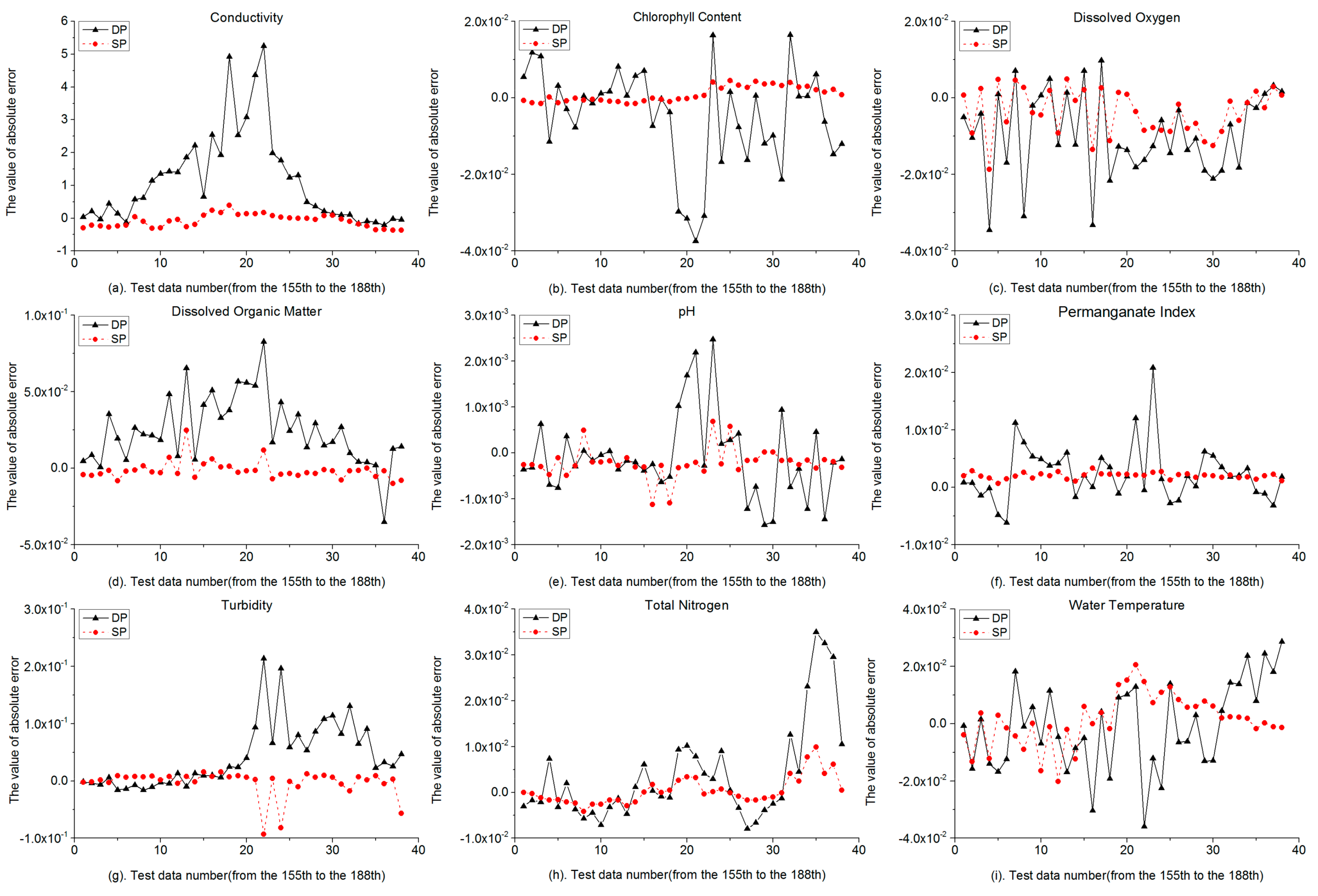
Note: Here “DP” = ”default predictors”, “SP” = ”selected predictors”.

, the RMSE and MAPE values of 9 water quality indicators used as the selected predictors were all less than the default predictors. Those forecast results are also shown in Figure 4 that 9 water quality indicators of the SP have smaller data variation ranges of the absolute errors that the curves were more stable than the DP. In DP, the maximum MAPE was 1.222% (TB), 2 were less than 0.1%, 6 were between 0.1% and 1%, 1 was over 1%. In SP, the maximum MAPE was 0.33% (TB), 8 were less than 0.1%, 1 was over 0.3%. The maximum RMSE of DP and SP was conductivity, the values were 1.8106 and 0.2087, respectively. According to previous research, turbidity can be influenced by various external and internal factors such as the dustfall, the temperature, and the water sample collection process may lead to lower forecast accuracy than other indicators. The data ranges of conductivity were from 450 to 781, which would cause the RMSE value of conductivity larger than other indicators. The fluctuating data change process would also lead to lower forecast accuracy in conductivity. However, when we select the pertinent predictors for conductivity, the MAPE value reduced significantly from 0.243% to 0.032%. Similar improvements also occurred on the dissolved organic matter and total nitrogen, the MAPEs reduced from 0.438% to 0.070% and 0.324% to 0.093%, respectively. When the inputs were the selected predictors, the forecast accuracy was higher than the default inputs.

Since the water quality indicators can be affected by various external and internal factors, if we used all the seven external environmental factors together as the predictors, the model would be not effective enough to forecast the water quality by the CS-BP model in this case study. Therefore, using the data pre-processing methods to select the new predictors was useful and effective, and we set the selected predictors as inputs in the next simulation.

5.2. Comparison of Different Models

Table 6. The RMSE and MAPE of water quality indicators of four models in Scenario 2.

Indicators	RMSE				MAPE
	PSO-BP	GRNN	BP	CS-BP	PSO-BP	GRNN	BP	CS-BP
CD	1.9634	40.0048	18.0959	0.2087	0.239	6.165	2.786	0.032
CC	0.0456	1.3176	0.9100	0.0022	0.489	16.516	10.321	0.030
DO	0.0220	0.4656	0.2358	0.0069	0.113	3.587	2.005	0.052
DOM	0.0428	2.0503	0.6965	0.0062	0.448	28.154	7.511	0.070
pH	0.0017	0.0484	0.0108	0.0004	0.018	0.505	0.115	0.004
PI	0.0080	0.2040	0.1222	0.0021	0.207	6.183	4.061	0.077
TB	0.0808	1.1002	0.4502	0.0234	1.456	25.149	11.248	0.330
TN	0.0075	0.1816	0.1443	0.003	0.237	6.740	4.735	0.093
WT	0.0564	0.8090	0.4518	0.0089	0.139	2.130	1.320	0.023

, Figure 5 and Figure 6 showed the forecast results of four models in Scenario 2.

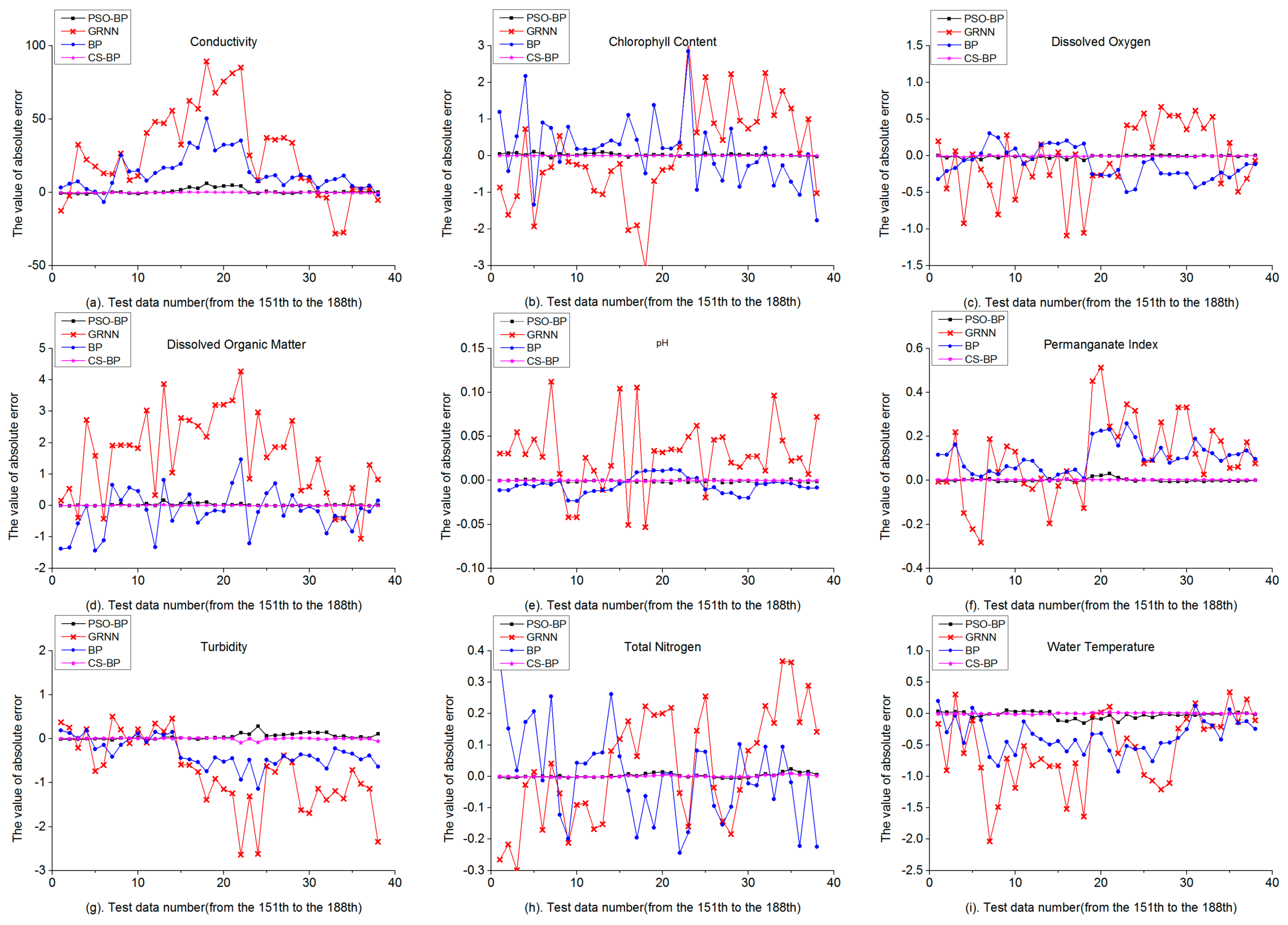
Compare the BP model and the GRNN model in Table 6, the RMSEs of 9 water quality indicators of the BP model were all less than those of the GRNN model, the maximum RMSE was 18.0959 (CD) of the BP model, while the maximum RMSE was 40.0048 (CD) of the GRNN model. The maximum MAPE of the GRNN model was 28.154% (DOM), 1 was less than 1%, 5 were between 1% and 10%, 1 was between 10% and 20%, 2 were over 20%. The maximum MAPE of the BP model was 11.248% (TB), 1 was less than 1%, 7 were between 1% and 10%, 1 was over 10%. All the MAPEs of 9 water quality indicators of the BP model were still less than those of the GRNN model. 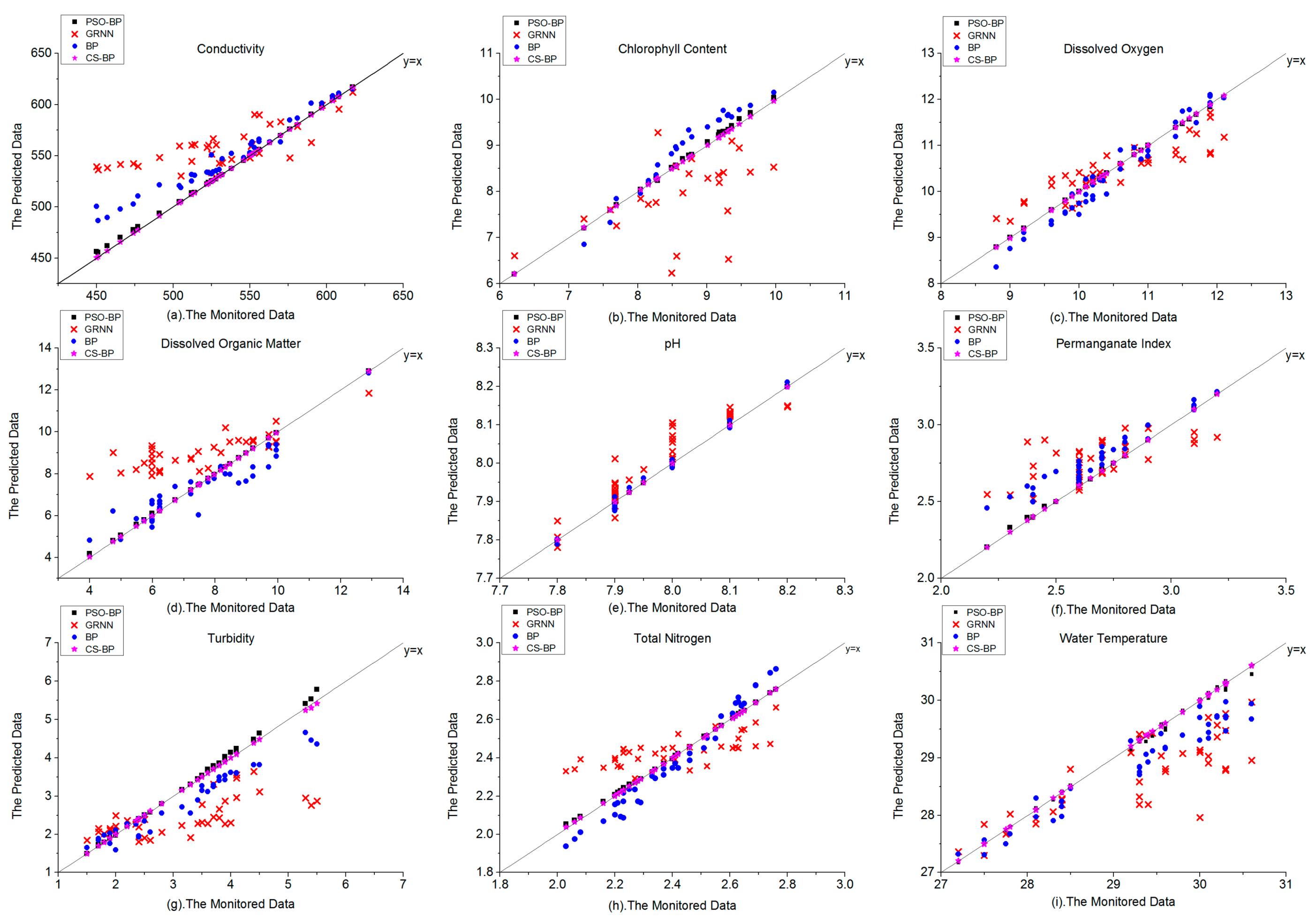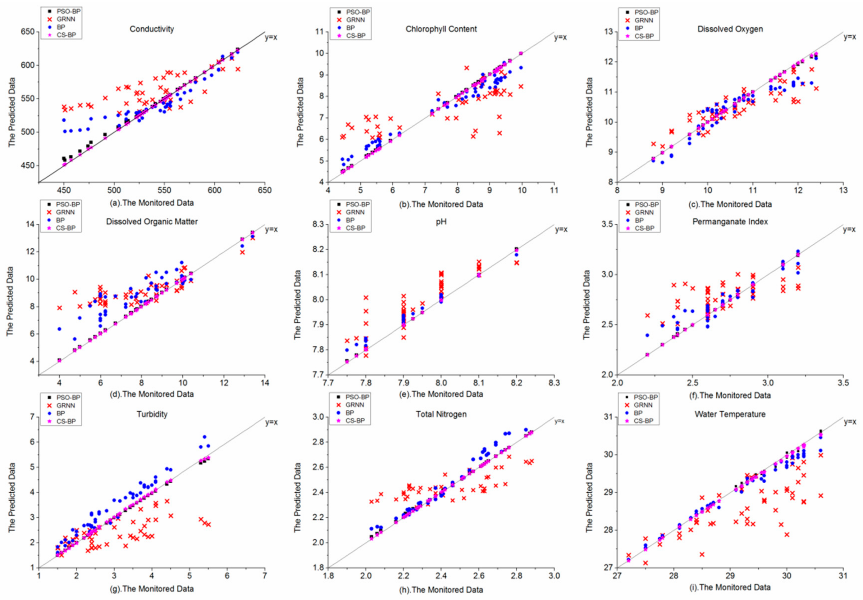The absolute error curves of the GRNN model were much more unstable than the BP model in Figure 5, the most violent absolute error curve was shown in Figure 5d, corresponding to the maximum MAPE of DOM in Table 6, 28.154%. Compared with the predicted data and the monitored data in Figure 6, the points of pH of the GRNN model in Figure 6e were concentrated on the Y = X line relatively well, corresponding to the lowest MAPE value of the other 8 indicators in Table 6. The points of the GRNN model and the BP model were more scattered in Figure 6b,d,g, corresponding to higher MAPE values than the other 6 indicators in Table 6. It showed that the GRNN model has larger absolute error at some data points and the forecast performance of the traditional BP model was better than the GRNN model in this case study.

The CS-BP model has the lowest RMSE and MAPE values of 9 water quality indicators in Table 6. The RMSEs of CD and CC of CS-BP model were significantly lower than those of the PSO-BP model, where the values were 0.2087:1.9634 and 0.0022:0.0456, respectively. The rest of the RMSEs of 7 indicators of CS-BP model were also lower than those of the PSO-BP model. The maximum RMSE of CS-BP model was 0.2087 (CD), while the PSO-BP model was 1.9634 (CD). The maximum MAPE of CS-BP model was 0.33% (TB), 8 were less than 0.1%, 1 was over 0.3%, while the maximum MAPE of PSO-BP model was 1.456% (TB), 1 was lower than 0.1%, 7 were between 0.1% and 1%, 1 was over 1%. Figure 6 showed that the distribution of the predicted data and monitored data of four models, the CS-BP model still maintained the highest forecast accuracy that the points were concentrated on the Y = X line relatively well. In Figure 6a,b,d,g, the PSO–BP model showed some certain errors compared with the forecast performance of the CS–BP model. The results indicated that compared with the PSO-BP model and the traditional BP model, the forecast accuracy of the CS-BP model in this case study was effectively improved.

5.3. Comparison of Different Data Proportion

Table 7. The RMSE of water quality indicators of four models in different data proportions in Scenario 3.

Indicators					RMSE
	Part A					Part B
	PSO-BP	GRNN	BP	CS-BP		PSO-BP	GRNN	BP	CS-BP
CD	12.2692	46.4205	30.3296	2.6889		3.1694	46.5036	26.1044	0.4218
CC	0.0252	1.1006	0.4114	0.0120		0.0260	1.2978	0.4118	0.0194
DO	0.0807	0.5245	0.2447	0.0684		0.0461	0.5055	0.3727	0.0271
DOM	0.043	1.6408	0.6390	0.0347		0.0480	1.8716	1.3641	0.0185
pH	0.0036	0.0643	0.0261	0.0005		0.0025	0.0670	0.0256	0.0014
PI	0.0122	0.2247	0.0943	0.0120		0.0044	0.2042	0.0869	0.0011
TB	0.0506	0.9962	0.6496	0.0236		0.0424	1.0139	0.4366	0.0266
TN	0.1016	0.3570	0.3004	0.0863		0.0089	0.1720	0.0893	0.0032
WT	0.1045	0.8092	0.2933	0.0697		0.0550	0.8450	0.1355	0.0334

Note: Part A and Part B present the data proportion for 130:58 (testing data: training data) and 140:48 (testing data: training data), respectively.

and

Table 8. The MAPE of water quality indicators of four models in different data proportions in Scenario 3.

Indicators					MAPE
	Part A					Part B
	PSO-BP	GRNN	BP	CS-BP		PSO-BP	GRNN	BP	CS-BP
CD	1.086	6.160	3.120	0.190		0.387	6.643	3.344	0.044
CC	0.251	13.006	4.588	0.163		0.329	15.058	5.105	0.207
DO	0.447	3.688	1.473	0.374		0.234	3.616	2.768	0.146
DOM	0.464	19.846	7.259	0.362		0.669	23.783	16.963	0.230
pH	0.032	0.630	0.252	0.004		0.022	0.688	0.272	0.014
PI	0.304	7.037	3.021	0.338		0.141	6.019	2.644	0.037
TB	0.952	27.59	24.087	0.510		0.646	22.447	14.195	0.576
TN	1.494	7.979	5.968	1.154		0.254	5.976	2.197	0.091
WT	0.353	2.217	0.832	0.164		0.149	2.247	0.444	0.092

Note: Part A and Part B present the data proportion for 130:58 (testing data: training data) and 140:48 (testing data: training data), respectively.

, Figure 7, Figure 8, Figure 9 and Figure 10 showed the forecast results of four models in Scenario 3.

In Table 7, all the RMSE in both Part A and Part B of the BP model were still lower than the GRNN model when the training data was reduced from 140 to 130. However, the RMSE values of those two models did not increase synchronously. The RMSEs of 3 indicators (DO, PI and TN) increased of the GRNN model from Part B to Part A, while the RMSEs of 6 indicators (CD, pH, PI, TB, TN and WT) increased of the BP model. In both Part A and Part B of Table 8, the maximum MAPE of the GRNN model was 27.59% (TB), 2 were less than 1%, 10 were between 1% and 10%, 3 were between 10% and 20%, 3 were over 20%, while the maximum MAPE of BP model was 24.087%(TB), 4 were less than 1%, 11 were between 1% and 10%, 2 were between 10% and 20%, only 1 was over 20%. These results indicated that when the training data were reduced, the forecast performances of the BP model and the GRNN model were not satisfactory. The worst forecast result was in the turbidity. The maximum increase of the MAPE of GRNN model and BP model was in turbidity. In the GRNN model, the MAPE of turbidity increased from 22.45% to 27.59%, an increase of 5.14%, and in the BP model, the MAPE of turbidity increased from 14.20% to 24.09%, an increase of 9.89%. In addition, the forecast results of the two models on dissolved organic matter (DO) and chlorophyll content (CC) were also worse than the rest of the 6 indicators. The results showed that the training data reduction has a significant impact on the GRNN model and BP model. When the training data were reduced, the accuracy of the GRNN and the traditional BP were very low and the results become unreliable. The traditional BP model and GRNN mode cannot show the ability to resist the decline of forecast accuracy caused by the reduction of training data. These results indicated that it is meaningful and necessary to improve the traditional BP model. Optimization algorithm can improve the forecast accuracy of the BP model, and can reduce the impact caused by the reduction of training data, to some certain extent.

Compared the RMSEs in Part A and Part B of the CS-BP model in Table 7, when the training data reduced from 140 to 130, all the RMSEs of the CS-BP model were still the lowest among the four models. The RMSEs of 6 indicators (CD, DO, DOM, PI, TN, and WT) in the CS-BP model increased from Part B to Part A, while the RMSEs of 7 indicators (CD, DO, pH, PI, TB, TN, and WT) of the PSO-BP model increased from Part B to Part A. Compared the RMSEs of CS-BP model in Part A with the PSO-BP model in Part B, the RMSEs of 5 indicators (CD, CC, DOM, pH and TB) were less than those of the PSO-BP model in Part B. In Table 8, the MAPEs of 6 indicators (CD, DO, DOM, PI, TN, and WT) increased in the CS-BP model from Part B to Part A, while 7 indicators increased in the PSO-BP model (CD, DO, pH, PI, TB, TN, and WT). The maximum MAPE of the CS-BP model in Part A was 1.154% (TN), 1 was lower than 0.1%, 6 were between 0.1% and 0.5%, 1 was between 0.5% and 1%, 1 was over 1%. The maximum MAPE of the PSO-BP model in Part B was 0.669% (DOM), 1 was lower than 0.1%, 6 were between 0.1% and 0.5%, 2 were between 0.5% and 1%. In addition, there were 5 indicators (CD, CC, DOM, pH, and TB) have lower MAPEs of the CS-BP model in Part A than those of the PSO-BP model in Part B. These results have shown that the CS-BP model still shows higher forecast accuracy than the PSO-BP model when the training data were reduced. In this case, when the training data of the CS-BP model was less the PSO-BP model, the forecast accuracy of some indicators are still higher than that of the PSO-BP model, which proved that the CS-BP model has a better ability to resist the impacts of training data reduction than the PSO-BP model.

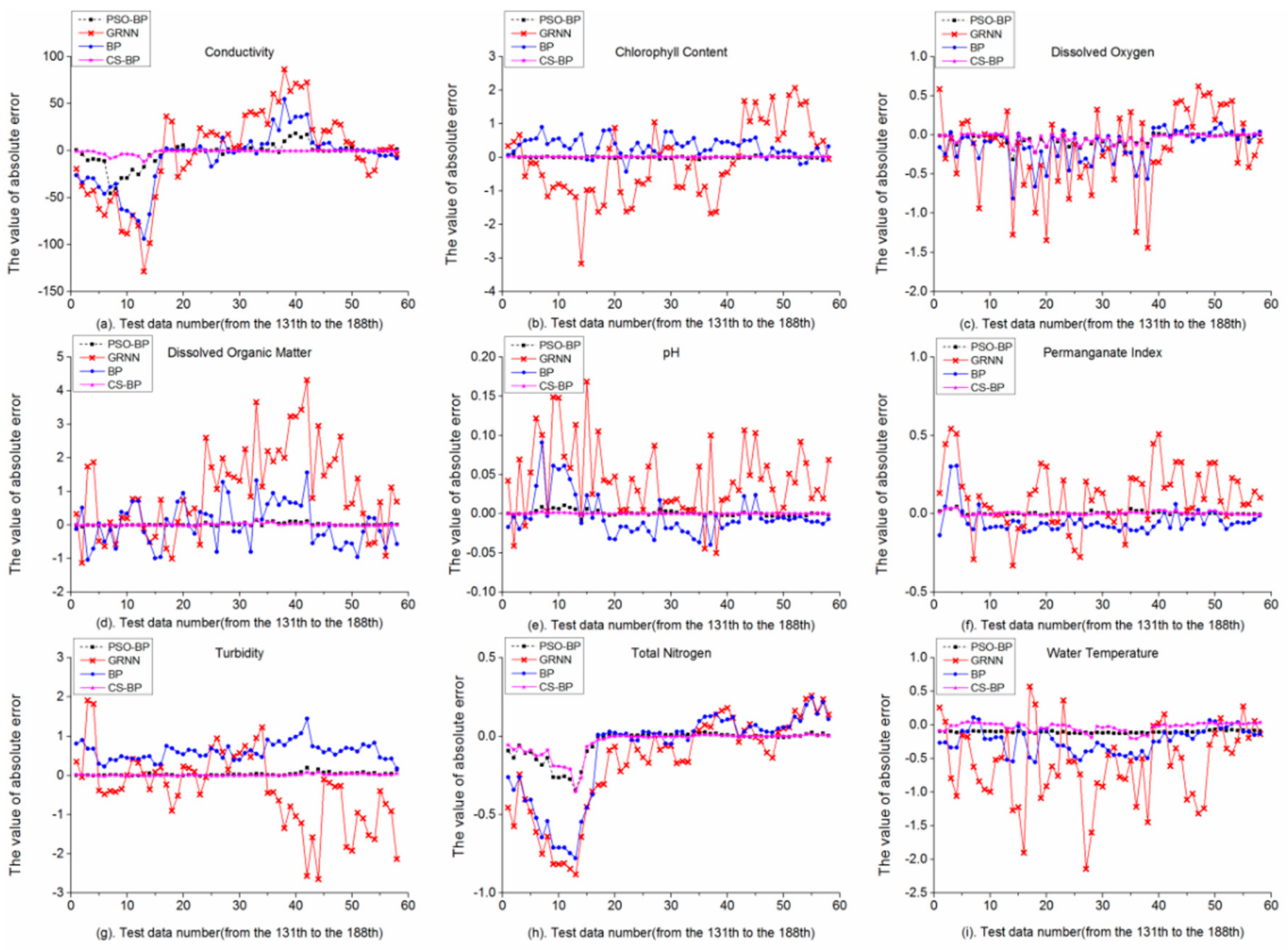
Figure 7 and Figure 8 showed that the absolute error curves of the GRNN model were more unstable than the BP model, corresponding to the MAPE values of the GRNN model in both Part A and Part B were larger than those of the BP model. In Figure 7, we see that the curves of the GRNN model were more volatile than the other 3 models. In Figure 7a, the maximum absolute errors of the GRNN model and the BP model were closed to 130 μs/cm and 95 μs/cm, respectively, and the MAPE values were almost 17% and 12%, respectively, at that data point. Similar phenomenon appeared in Figure 7h, the MAPEs of total nitrogen of the GRNN model and the BP model were almost 22% and 19%, respectively, at the maximum absolute errors data point. The maximum increase of the MAPE of the CS-BP model and the PSO-BP model was TN, from 0.091% to 1.154%, from 0.254% to 1.494%, respectively, corresponding to the absolute error curves have obvious inflection points in Figure 7h. We speculate that the lack of training data was the major problem of significant absolute errors and inflection points in the previous part of the curves. 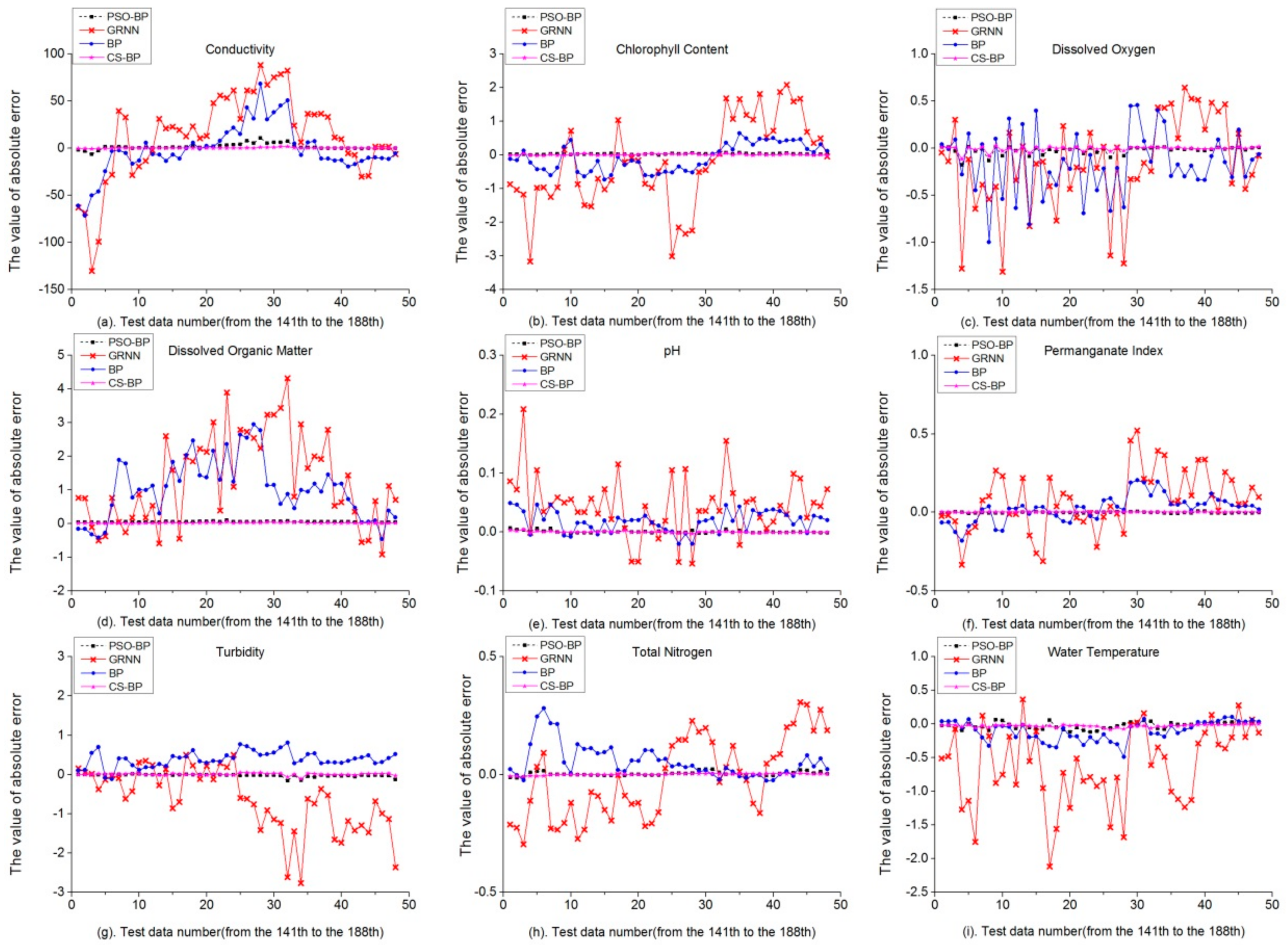In Figure 8, the absolute error curves of the GRNN model and the BP model were still unstable than the PSO-BP model and the CS-BP model, some data points have serious forecast errors. These results indicated that neither the GRNN model nor the BP model can have forecast results in Scenario 3. In Figure 8h, there was no obvious inflection point of the CS-BP model, but it still exists in the PSO-BP model. The result also reflected the ability of the CS-BP model to resist training data shortage. Overall, Figure 7 and Figure 8 indicated that the curves of the PSO-BP model and the CS-BP model were stable, representing more accurately forecast results. Meanwhile, the CS-BP model shows better adaptability than the PSO-BP model, when training data were reduced.

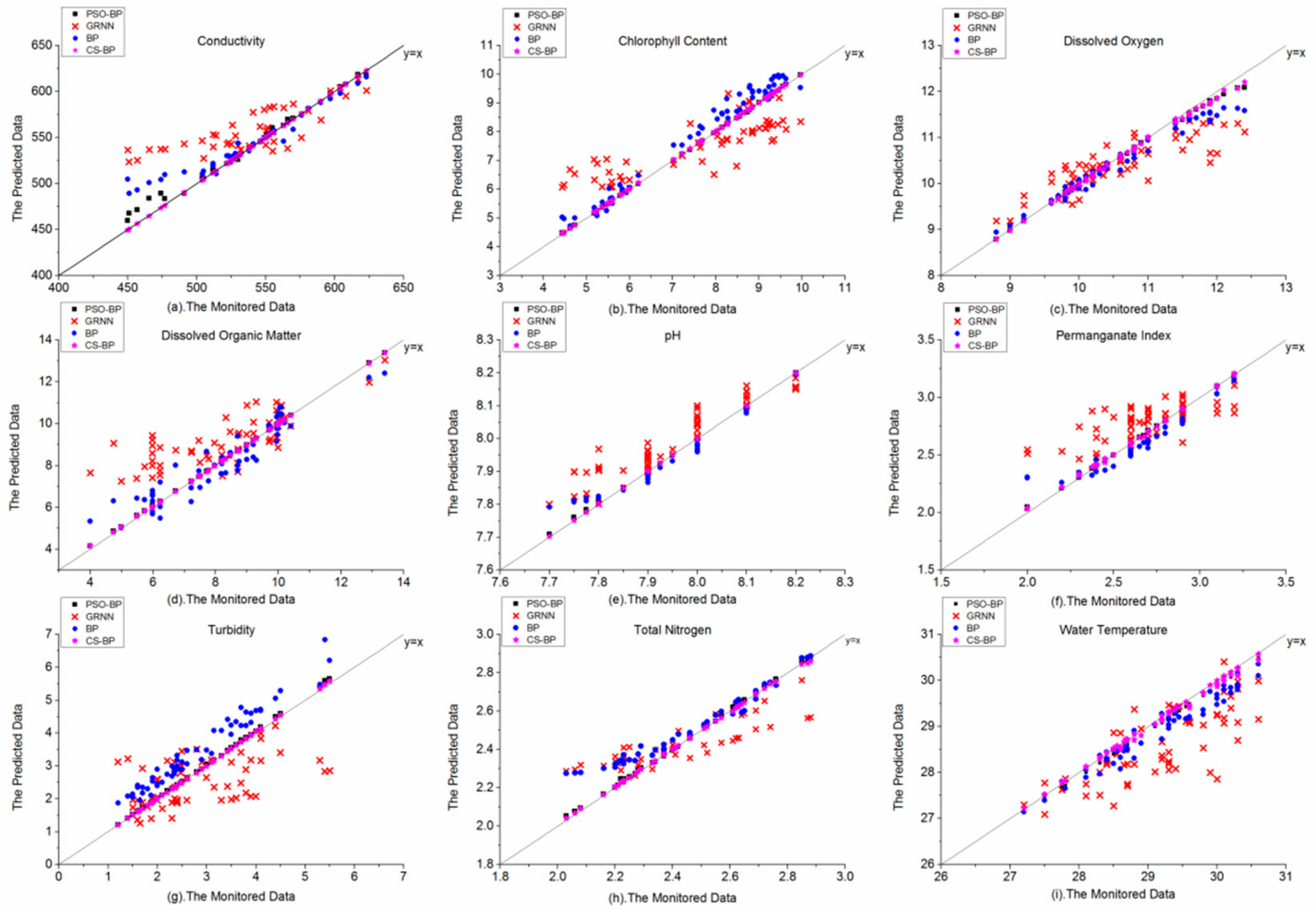
Figure 9 and Figure 10 showed that the distribution of the predicted data and monitored data of the GRNN model and the BP model are more scattered than the CS-BP model and the PSO-BP model. In Figure 9, the points of the GRNN model of Figure 9b,d,g were very fragmented, corresponding to higher MAPEs in CC, DOM, and TB than other models in Table 8. Similar phenomena occurred in Figure 10, these results indicated that the forecast performance of the GRNN model was poor in this case, using the CS algorithm to improve the GRNN model needs to be studied in the future. In addition, although the traditional BP model performed more accurately than the GRNN model in this case, the accuracy of some indicators such as turbidity and chlorophyll content still unsatisfactory as the Figure 9b,d and Figure 10b,d have shown. The training data reduction lead to the reduction of forecast accuracy. When the CS-BP model has less training data than the PSO-BP model, the CS-BP model still has better forecast accuracy than the PSO-BP model in some water quality indicators (CD, CC, DOM, pH, and TB).

In summary, the CS-BP model performed best in forecasting each water quality indicator in this case and the CS-BP model can be used to forecast daily water quality with limited observed data condition, such as the South-to-North Water Diversion Project of China.

5.4. Discussion of the CS-BP Model

Comparing the forecast performance of the CS-BP model and the BP model, it can be seen that the forecast accuracy of the CS-BP model is much higher than that of traditional BP model. The reason is that the traditional BP models have some intrinsic drawbacks such as calculation instability and low convergence efficiency, which will reduce the forecast accuracy of the models. The application of intelligent optimization algorithm is more efficient than the traditional BP model random calculation, and can quickly obtain the weights and thresholds for a specific problem, which is also the current research hotspot of the BP model. Comparing the CS-BP model with PSO-BP model, it can be seen that the calculation flows of the two models are basically the same, and the methods and principles are also similar. The difference of the accuracy of the forecast results of the two models may be due to the difference of the optimization algorithm themselves. The PSO was invented earlier than the CS, and the traditional PSO also has some computational defects. Over the years, many scholars have studied the improvement of the PSO. The optimization mechanism of the CS algorithm ensures that the algorithm has the advantages of higher search efficiency and faster calculation speed, which is also the reason that the CS-BP model has higher forecast accuracy than the PSO-BP model. In previous research, many scholars have proved that the CS algorithm is more efficient than the PSO. However, the CS algorithm is not an algorithm without defects. Later, more in-depth research on the improvement of the CS algorithm is needed.

There are also some drawbacks in this study, such as the lack of in-depth study on the impact of land management on the water quality of the MR SNWDPC, as well as an in-depth study on the regularity of water quality periodic changes; these are the research directions for further study. Some other research directions are also to improve CS algorithm and its coupling with some mechanism models, and to study the impact of various environmental factors on the South-to-North Water Diversion Project. According to this study, the CS-BP model can not only be applied to water quality forecast, but also be worth popularizing to other forecast problems, such as food production prediction, population prediction, and other issues when input factors are selected appropriately.

6. Conclusions

In this paper, a new forecast model, called the CS-BP model, was applied to forecast the daily water quality of the South-to-North Water Diversion Project of China. The model was based on the traditional BP network, the Cuckoo Search algorithm was used to optimize the initial weights $w_{ij}$ and $w_{jk}$, the thresholds $a$ and $b$ of the traditional BP model. Nine water quality indicators, including conductivity, chlorophyll content, dissolved oxygen, dissolved organic matter, pH, permanganate index, turbidity, total nitrogen and water temperature were the predictand. Seven external environmental factors, including air temperature, PM2.5, rainfall, sunshine duration, water flow, wind velocity and water vapor pressure were the default predictors to the model. A data pre-processing method was used to select pertinent predictors for each water quality indicator. The traditional BP model, the PSO-BP model and the GRNN model were used to compare the forecast performance with the CS-BP model. Three simulation scenarios were set up. The result of Scenario 1 showed that using the data pre-processing method to select the predictors for the model was effective that could improve the forecast accuracy of the model, 9 water quality indicators that used the selected predictors were all less than the default predictors. The forecast results of the CS-BP model were satisfactory, which have the lowest RMSE and MAPE values in all water quality indicators among the four models in Scenario 2. Five water quality indicators have lower RMSE and MAPE values of CS-BP model than those of PSO-BP model while the training data was 130, 140, respectively. It showed that the CS-BP model can maintain higher forecast accuracy than other three models with limited observed data in this case. It can be concluded that the CS-BP model is a feasible and effective tool to forecast daily water quality effectively with limited observed data under normal operating conditions, and can be applied to water security management of the South-to-North Water Diversion Project of China. The impact of different environmental factors on the South-to-North Water Diversion Project and the improvement of the CS-BP model will be discussed in the future.

References

1. Weerasekara, P. The united nations world water development report 2017 wastewater: The untapped resource. Future Food 2017, 5, 80–81. [Google Scholar]
2. Odagiri, M.; Cahyorini, K.A.; Cronin, A.A.; Gressando, Y.; Hidayat, I.; Utami, W.; Widowati, K.; Roshita, A.; Soeharno, R.; Warouw, S.P. Water, sanitation, and hygiene services in public health-care facilities in indonesia: Adoption of world health organization/united nations children’s fund service ladders to national data sets for a sustainable development goal baseline assessment. Am. J. Trop. Med. Hyg. 2018, 99, 546–551. [Google Scholar] [CrossRef] [PubMed]
3. Dou, M.; Wang, Y.Y. The construction of a water rights system in china that is suited to the strictest water resources management system. Water Sci. Technol. Water Supply 2017, 17, 238–245. [Google Scholar] [CrossRef]
4. Wang, C.; Wang, Y.Y.; Wang, P.F. Water quality modeling and pollution control for the eastern route of south to north water transfer project in china. J. Hydrodyn. 2006, 18, 253–261. [Google Scholar] [CrossRef]
5. Shao, D.G.; Wang, Z.M.; Wang, B.; Luo, W.W. A water quality model with three dimensional variational data assimilation for contaminant transport. Water Resour. Manag. 2016, 30, 4501–4512. [Google Scholar] [CrossRef]
6. Lintern, A.; Webb, J.A.; Ryu, D.; Liu, S.; Bende-Michl, U.; Waters, D.; Leahy, P.; Wilson, P.; Western, A.W. Key factors influencing differences in stream water quality across space. Wiley Interdiscip. Rev.-Water 2018, 5, e1260. [Google Scholar] [CrossRef]
7. Fard, A.K.; Akbari-Zadeh, M.R. A hybrid method based on wavelet, ann and arima model for short-term load forecasting. J. Exp. Theor. Artif. Intell. 2014, 26, 167–182. [Google Scholar] [CrossRef]
8. Pekárová, P.; Onderka, M.; Pekár, J.; Ák, P.R.; Miklánek, P. Prediction of water quality in the danube river under extreme hydrological and temperature conditions. J. Hydrol. Hydromech. 2009, 57, 3–15. [Google Scholar] [CrossRef]
9. Singh, K.P.; Basant, A.; Malik, A.; Jain, G. Artificial neural network modeling of the river water quality—A case study. Ecol. Model. 2009, 220, 888–895. [Google Scholar] [CrossRef]
10. Durdu, O.F. Spatial predictions of surface water quality based on general regression neural network: A case study of the buyuk menderes catchment, turkey. Fresenius Environ. Bull. 2009, 18, 1603–1613. [Google Scholar]
11. Mehta, R.; Rajpal, N.; Vishwakarma, V.P. Sub-band discrete cosine transform-based greyscale image watermarking using general regression neural network. Int. J. Signal Imaging Syst. Eng. 2015, 8, 380–389. [Google Scholar] [CrossRef]
12. Su, J.Q.; Wang, X.; Zhao, S.Y.; Chen, B.; Li, C.H.; Yang, Z.F. A structurally simplified hybrid model of genetic algorithm and support vector machine for prediction of chlorophyll a in reservoirs. Water 2015, 7, 1610–1627. [Google Scholar] [CrossRef]
13. Wang, Z.M.; Shao, D.G.; Yang, H.D.; Yang, S. Prediction of water quality in south to north water transfer project of china based on ga-optimized general regression neural network. Water Sci. Technol.-Water Supply 2015, 15, 150–157. [Google Scholar] [CrossRef]
14. Gotovtsev, A.V. Modification of the streeter-phelps system with the aim to account for the feedback between dissolved oxygen concentration and organic matter oxidation rate. Water Resour. 2010, 37, 245–251. [Google Scholar] [CrossRef]
15. Deliman, P.; Gerald, J. Application of the two-dimensional hydrothermal and water quality model, ce-qual-w2, to the chesapeake bay—Conowingo reservoir. Lake Reserv. Manag. 2002, 18, 10–19. [Google Scholar] [CrossRef]
16. Zhu, W.B.; Wang, H.X.; Liu, C.; Zhang, J.; Liang, S. Improvement of river water quality by aeration: Wasp model study. Environ. Sci. 2015, 36, 1326–1331. [Google Scholar]
17. Guo, F.; Hanfei, Q.U.; Zeng, H.; Cong, P.; Geng, X. Flood routing numerical simulation of flood storage area based on mike21 fm model. Water Resour. Power 2013, 5, 009. [Google Scholar]
18. Ortolani, V. Land use and its effects on water quality using the basins model. Environ. Earth Sci. 2014, 71, 2059–2063. [Google Scholar] [CrossRef]
19. Srinivasan, R.; Arnold, J.G. Integration of a basin-scale water quality model with gis. Jawra J. Am. Water Resour. Assoc. 2010, 30, 453–462. [Google Scholar] [CrossRef]
20. Zhou, G.; Wang, H.Y.; Chun-Xue, H.U.; Cheng, X.R.; Cai, W.W. Application of grey information renewal gm (1,1) model in prediction of medium and long-term urban water demand. China Rural Water Hydropower 2005, 8, 16–18. [Google Scholar]
21. Karmakar, S.; Mujumdar, P.P. Grey fuzzy optimization model for water quality management of a river system. Adv. Water Resour. 2006, 29, 1088–1105. [Google Scholar] [CrossRef]
22. Khalil, B.M.; Awadallah, A.G.; Karaman, H.; Elsayed, A. Application of artificial neural networks for the prediction of water quality variables in the nile delta. J. Water Resour. Prot. 2012, 4, 388–394. [Google Scholar] [CrossRef]
23. Nasir, M.F.M. Artificial neural networks combined with sensitivity analysis as a prediction model for water quality index in juru river, malaysia. Int. J. Environ. Prot. 2011, 1, 1–8. [Google Scholar] [CrossRef]
24. Zhong, W.; Li, G.; Luo, Y.; Wang, W.; Sun, Y.; Li, B.; Zhao, B. Water quality prediction of guanyin mountain in tien lake based on markov grey residual error modified model. Environ. Sci. Manag. 2016, 41, 80–84. [Google Scholar]
25. Zhang, L.; Zou, Z.; Shan, W. Development of a method for comprehensive water quality forecasting and its application in miyun reservoir of beijing, china. J. Environ. Sci.-China 2017, 56, 240–246. [Google Scholar] [CrossRef] [PubMed]
26. Wang, X.; Lv, J.; Xie, D. A hybrid approach of support vector machine with particle swarm optimization for water quality prediction. In Proceedings of the International Conference on Computer Science & Education, Hefei, China, 24–27 August 2010; pp. 1158–1163. [Google Scholar]
27. Sahoo, K.; Mani, S.; Das, L.; Bettinger, P. Gis-based assessment of sustainable crop residues for optimal siting of biogas plants. Biomass Bioenergy 2018, 110, 63–74. [Google Scholar] [CrossRef]
28. Bayram, A.; Kankal, M.; Önsoy, H. Estimation of suspended sediment concentration from turbidity measurements using artificial neural networks. Environm. Monit. Assess. 2012, 184, 4355–4365. [Google Scholar] [CrossRef] [PubMed]
29. Wang, Z. Prediction and comparative analysis of water quality based on ga-bp and multi-hidden-layer bp network model. J. Water Resour. Water Eng. 2013, 3, 035. [Google Scholar]
30. Ding, Y.R.; Cai, Y.J.; Sun, P.D.; Chen, B. The use of combined neural networks and genetic algorithms for prediction of river water quality. J. Appl. Res. Technol. 2014, 12, 493–499. [Google Scholar] [CrossRef]
31. Yan, J.X.; Yu, L.J.; Mao, W.W.; Cao, S.Q. Study on prediction model of dissolved oxygen about water quality monitoring system based on bp neural network. Adv. Mater. Res. 2014, 912–914, 1407–1411. [Google Scholar] [CrossRef]
32. Tian, J.; Cao, D.; Hainan, L.I. Application of lm-bp neural network in water quality prediction for yu qiao reservoir. Water Resour. Inf. 2010, 4, 013. [Google Scholar]
33. Wei, H.; Li, W.; Zhang, S.; Wang, G. Prediction of reservoir water quality in northeast china with bp neural network model. Water Technol. 2009, 1, 005. [Google Scholar]
34. Xu, L.; Fang, Z.G.; Liu, S.F. Quality prediction model by using pso-bp neural network. Ind. Eng. J. 2012, 4, 006. [Google Scholar]
35. Cai-Hong, S.U.; Xiang, N.; Lin, M.J.; Department, A.; University, F. Dissolved oxygen prediction based on artificial bee colony optimization algorithm and bp neural network. Comput. Simul. 2013, 30, 325–329. [Google Scholar]
36. Yang, X.S.; Deb, S. Cuckoo search via levey flights. In Proceedings of the World Congress on Nature & Biologically Inspired Computing (Nabic 2009), Coimbatore, India, 9–11 December 2009. [Google Scholar]
37. Yang, X.S.; Deb, S.; Karamanoglu, M.; He, X. Cuckoo search for business optimization applications. In Proceedings of the National Conference on Computing and Communication Systems (NCCCS), West Bengal, India, 21–22 November 2012. [Google Scholar]
38. Musigawan, P.; Chiewchanwattana, S.; Sunat, K. Improved differential evolution via cuckoo search operator. In Proceedings of the Neural Information Processing, Iconip 2012, Pt I, Doha, Qatar, 12–15 November 2012; Volume 7663, pp. 465–472. [Google Scholar]
39. Kishnani, M.; Pareek, S.; Gupta, R. Optimal tuning of pid controller by cuckoo search via levy flights. In Proceedings of the 2014 International Conference on Advances in Engineering and Technology Research (ICAETR), Singapore, 29–30 March 2014. [Google Scholar]
40. Han, W.H.; Xu, J.; Zhou, M.C.; Tian, G.Y.; Wang, P.; Shen, X.H.; Hou, E. Cuckoo search and particle filter-based inversing approach to estimating defects via magnetic flux leakage signals. IEEE Trans. Magn. 2016, 52, 1–11. [Google Scholar] [CrossRef]
41. Marichelvam, M.K.; Prabaharan, T.; Yang, X.S. Improved cuckoo search algorithm for hybrid flow shop scheduling problems to minimize makespan. Appl. Soft Comput. 2014, 19, 93–101. [Google Scholar] [CrossRef]
42. Chen, X.J.; Jin, S.Q.; Qin, S.S.; Li, L.P. Short-term wind speed forecasting study and its application using a hybrid model optimized by cuckoo search. Math. Prob. Eng. 2015, 2015, 608597. [Google Scholar] [CrossRef]
43. Ming, B.; Chang, J.X.; Huang, Q.; Wang, Y.M.; Huang, S.Z. Optimal operation of multi-reservoir system based-on cuckoo search algorithm. Water Resour. Manag. 2015, 29, 5671–5687. [Google Scholar] [CrossRef]
44. Kennedy, J.; Eberhart, R.C.; Shi, Y. Swarm Intelligence; Morgan Kaufmann Publishers Inc.: Burlington, MA, USA, 2001; pp. 187–219. [Google Scholar]
45. Li, H.Z.; Guo, S.; Li, C.J.; Sun, J.Q. A hybrid annual power load forecasting model based on generalized regression neural network with fruit fly optimization algorithm. Knowl.-Based Syst. 2013, 37, 378–387. [Google Scholar] [CrossRef]
46. Copetti, D.; Carniato, L.; Crise, A.; Guyennon, N.; Palmeri, L.; Pisacane, G.; Struglia, M.V.; Tartari, G. Impacts of Climate Change on Water Quality; Springer: Dordrecht, The Netherlands, 2013; pp. 307–332. [Google Scholar]
47. Wilby, R.L.; Whitehead, P.G.; Wade, A.J.; Butterfield, D.; Davis, R.J.; Watts, G. Integrated modelling of climate change impacts on water resources and quality in a lowland catchment: River kennet, UK. J. Hydrol. 2006, 330, 204–220. [Google Scholar] [CrossRef]
48. Li, K.; Liu, X.; Ling, S.; Gong, Y.; Lu, C.; Ping, Y.; Tian, C.; Zhang, F. Response of alpine grassland to elevated nitrogen deposition and water supply in china. Oecologia 2015, 177, 65–72. [Google Scholar] [CrossRef] [PubMed]
49. Delpla, I.; Jung, A.V.; Baures, E.; Clement, M.; Thomas, O. Impacts of climate change on surface water quality in relation to drinking water production. Environ. Int. 2009, 35, 1225–1233. [Google Scholar] [CrossRef] [PubMed]
50. Chen, J.; Gao, X.; He, D.; Xia, X. Nitrogen contamination in the yangtze river system, China. J. Hazard. Mater. 2000, 73, 107–113. [Google Scholar]
51. Lamon, L.; Dalla, V.M.; Critto, A.; Marcomini, A. Introducing an integrated climate change perspective in pops modelling, monitoring and regulation. Environ. Pollut. 2009, 157, 1971–1980. [Google Scholar] [CrossRef] [PubMed]
52. Ren, N.; Yan, G.; Ma, J.; Li, Y. The study on the influence of environmental factors of the sumberged macrophytes in the east lake. Wuhan Univ. J. 1996, 42, 213–218. [Google Scholar]
Figure 1. The flow chart of back propagation neural network that is optimized by the Cuckoo Search algorithm (CS-BP) model.
Water 10 01471 g001
Figure 2. The flow chart of PSO-BP model.
Water 10 01471 g002
Figure 3. The flow chart of Generalized Regression Neural Network (GRNN) model.
Water 10 01471 g003
Figure 4. The absolute errors of water quality indicators of DP and SP using CS-BP model.
Water 10 01471 g004
Figure 5. The absolute errors of water quality indicators of four models in Scenario 2.
Water 10 01471 g005
Figure 6. The comparison of predicted data and monitored data of water quality indicators of four models in Scenario 2.
Water 10 01471 g006
Figure 7. The absolute errors of water quality indicators of four models of part A in Scenario 3.
Water 10 01471 g007
Figure 8. The absolute errors of water quality indicators of four models of part B in Scenario 3.
Water 10 01471 g008
Figure 9. Comparison result of predicted and monitored data of water quality indicators of four models of part A in Scenario 3.
Water 10 01471 g009
Figure 10. Comparison results of predicted and monitored data of water quality indicators of four models of part B in Scenario 3.
Water 10 01471 g010