Novel Ensembles of Deep Learning Neural Network and Statistical Learning for Flash-Flood Susceptibility Mapping


1
Research Institute of the University of Bucharest, 90-92 Sos. Panduri, 5th District, 050663 Bucharest, Romania
2
National Institute of Hydrology and Water Management, București-Ploiești Road, 97E, 1st District, 013686 Bucharest, Romania
3
Institute of Research and Development, Duy Tan University, Da Nang 550000, Vietnam
4
Geographic Information System Group, Department of Business and IT, University of South-Eastern Norway, N-3800 Bø i Telemark, Norway
*
Authors to whom correspondence should be addressed.
Water 2020, 12(6), 1549; https://0-doi-org.brum.beds.ac.uk/10.3390/w12061549
Submission received: 16 January 2020
/
Revised: 4 March 2020
/
Accepted: 5 March 2020
/
Published: 29 May 2020
(This article belongs to the Special Issue Droughts and Floods Assessment and Monitoring Using Remote Sensing and Geospatial Techniques)
Abstract
:This study aimed to assess flash-flood susceptibility using a new hybridization approach of Deep Neural Network (DNN), Analytical Hierarchy Process (AHP), and Frequency Ratio (FR). A catchment area in south-eastern Romania was selected for this proposed approach. In this regard, a geospatial database of the flood with 178 flood locations and with 10 flash-flood predictors was prepared and used for this proposed approach. AHP and FR were used for processing and coding the predictors into a numeric format, whereas DNN, which is a powerful and state-of-the-art probabilistic machine leaning, was employed to build an inference flash-flood model. The reliability of the models was verified with the help of Receiver Operating Characteristic (ROC) Curve, Area Under Curve (AUC), and several statistical measures. The result shows that the two proposed ensemble models, DNN-AHP and DNN-FR, are capable of predicting future flash-flood areas with accuracy higher than 92%; therefore, they are a new tool for flash-flood studies.
1. Introduction
As a result of the climatic changes that occurred during in recent years as well as of the massive changes in land use, a significant growth in the number of extreme meteorological and hydrological phenomena can be observed [1]. Thus, the increase in the global average temperature, which determines a surplus of energy in the atmosphere, and the conversion of more and more natural surfaces into built areas, are the leading causes of multiplying the number of floods and flash-floods throughout the world [2]. Popular floods and flash-floods are considered among the most devastating hazards [2,3]. Worldwide, these natural hazards cause multiple economic losses annually, affecting over 200 million people [4,5]. Flash-floods are defined as the rapid onset, usually up to 6 h, of the river level and flow, with high flooding potential in the areas where the slope angle allows water accumulation and the exceedance of the river banks [6]. Among the flash-floods triggering causes, heavy rainfalls rank the first, followed by the snow melting process and the breaking of dams [7]. The mitigation of flash-floods’ adverse effects requires the appropriate structural and non-structural measures.
The delimitation of the areas susceptible to flash-floods triggering is one of the essential non-structural measures that can be adopted [8]. Precise detection of surfaces susceptible to flash-floods generation is the basis for issuing the forecasts and warnings, which can further help to decrease the number of material damages and the number of casualties [9,10,11]. With the development of computerized analysis techniques, the number of studies that addressed the assessment of flash-flood susceptibility has increased significantly. A first method intended to evaluate the flash-flood potential for a specific territory is represented by the Flash-Flood Potential Index (FFPI), which was defined and proposed by Greg Smith [12]. The major drawback of this method, taken over by other researchers from the US [13,14,15] and other countries [2,16,17,18,19,20], is the assignment of equal weights for all the flash-floods predictors involved in the GIS workflow that was developed for FFPI computation.
A first attempt at weighting the flash-flood predictors from a statistical point of view was carried out by Costache and Zaharia [21], which determined the FFPI values within Bâsca Chiojdului catchment (Romania) through the combined use of bivariate statistical techniques with GIS specific ones. Moreover, for the FFPI assessment, the authors of the study above have taken into account the presence of the surfaces previously affected by torrential phenomena. These bivariate statistical methods are frequently involved in the studies concerning the computation of susceptibility to landslides and normal floods. In many cases, these techniques were associated with other complex models such as random forest, classification and regression trees, support vector machine, logistic regression, k-NN, and artificial neural networks [2,8,22,23,24,25,26,27,28,29]. The main advantage of these methods is its high degree of accuracy and the objectivity of the results, which can be explained by the fact that in the training process, they consider the surfaces previously affected by the natural hazards whose susceptibility is analyzed.
Along with the methods based on the use of the past phenomena location, within the vast field represented by the assessment of susceptibility to natural hazards, a high number of studies have been based on the weighting of predictors only based on expert judgment. In this regard, the most popular method is the Analytical Hierarchy Process [30,31,32]. In this context, in terms of flash-floods susceptibility assessment, we consider that there is a need for a comparison between the prediction capabilities of these two model types. Therefore, the present study aimed to estimate the Flash-Flood Potential Index by mean of a novel ensemble approach based on the hybrid combination of Deep Neural Network (DNN), on the one hand, and the Analytical Hierarchy Process (AHP) and the Frequency Ratio (FR), on the other hand. An ROC Curve, together with several statistical measures, were used to validate the results and to compare the reliability of the applied models.
2. Background of the Algorithms Used
2.1. Deep Neural Network
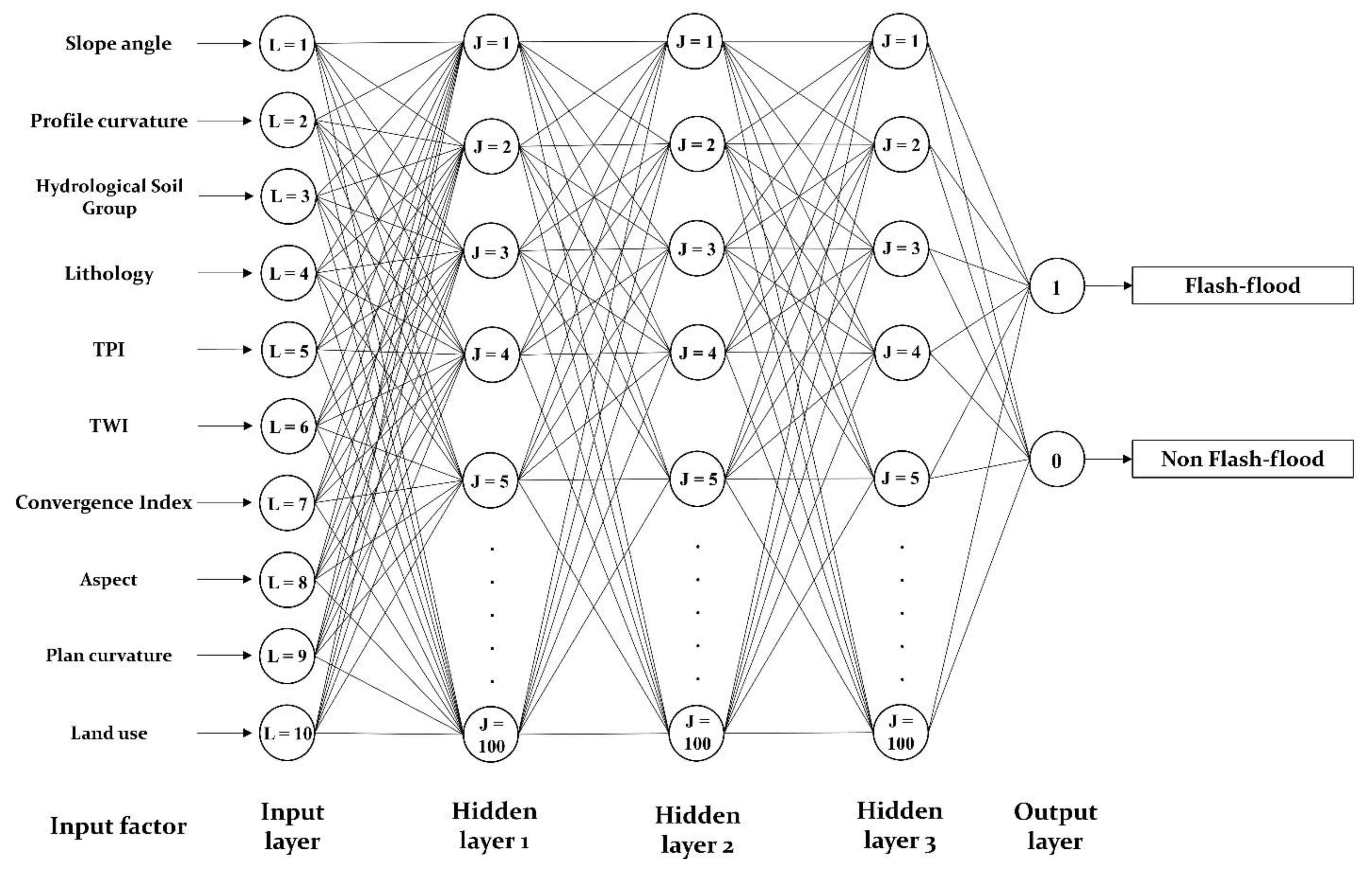
Unlike simple neural networks whose architecture contains a single hidden layer of neurons, the DNN has a feed-forward structure, which, along with input and output layers, contains two or more hidden layers [33]. Because the presence of multiple hidden layers is intended to solve complex classification problems, DNN models are considered to be more powerful and more efficient than simple neural networks [34]. In the present case, in Figure 1, the DNN architecture used in the present research is schematically represented to determine susceptibility to flash-floods. The input layer will contain information regarding the flash-flood predictors, which will be forwarded to hidden layers where this information will be analyzed and processed. The signals processed by hidden layers will be further sent to the output layer containing the negative class (non-flash-flood locations) and positive class (flash-flood locations) [35]. Further, using the back-propagation algorithm, the output error will be transmitted back from the output layer to the hidden layers. In the classification problems, the back-propagation algorithm is frequently used to train the feed-forward neural networks. In terms of the DNN, this algorithm calculates the gradient of the loss function with respect to each weight by the chain rule and avoids the redundant computations within the intermediate factors of this chain rule [36].
To process the received information, each neuron contained by the hidden layers will be applied to an activation function. In the present situation in which the deep neural network will use, for training, the vanishing gradient with the back-propagation algorithm, the activation function represented by the Rectified Linear Unit (ReLU) [35] will be employed. This function facilitates the determination of an optimal trade-off between the complexity, which is measured in terms of the number of nonzero weights of the network, and the approximation fidelity of neural networks when piecewise constant functions is approximated [37]. It should also be mentioned that there is a general agreement in the literature according to which ReLU can approximate more efficiently the smooth function than shallow networks [38]. ReLU function, which is expressed in Equation (1) will significantly reduce the vanishing gradient.
where x highlights the input signal received by a neuron and r denotes the ReLU function.
The use of the back-propagation algorithm requires the derivative of the ReLU function, which can be obtained as follows:
The difference between the flood inventories and the estimated floods is to reduce in the training procedure of DNN, by using the weights of the connections between the layers. In this regard, this difference, which is reduced through the back-propagation algorithm, will be highlighted by the cross-entropy function (E). In the present study, the cross-entropy function, which is usually used as a loss function, will be involved in the frame-leveling training. Remarkably, the cross-entropy function has a high contribution to the success of DNN [39]. The cross-entropy function has the following form:
where N is the total flash-flood points in the training sample; M is the flash-flood values, while P is the predicted flash-flood values.
Further, the training of the deep neural network in this research was done through the adaptive moment (Adam) estimation method, which combines the advantages of gradient descend with the momentum model and RMSProp model [40]. Adam is an algorithm used in the stochastic optimization process. It is considered that the Adam method is more performant than other stochastic optimization models and can achieve outstanding results [40]. The following formula can express the gradient used by the back-propagation procedure:
where m is a training sample ; T(i) (i = 1, 2, …, m) are the flash-flood; and L represents the cost function; C = 2 is the output classes, non-flash-flood and flash-flood; w highlights the network weights.
Using Adam, the first and second moment are estimated through the exponential moving averages, which are calculated with the following formulas [36]:
where m and v represent the moving averages, g is the gradient on the current mini-batch, and represents new hyper-parameters introduced within the algorithm. has a default value of 0.9 while has a default value of 0.999.
The bias correction for the first and second moment will be done with the help of the following formulas:
Further, using the moving averages, the network weights can be updated as follows [36]:
where is the model weight, is the learning rate and is equal to 0.001, and is used for the numerical stability and is equal to
Equation (10) ensures the update of the DNN parameters:
2.2. Analytical Hierarchy Process
Developed and proposed by Saaty [41], AHP allows us to analyze and resolve the problems in a flexible and easy-to-understand way. A characteristic of this multicriteria decision-making approach is represented by the participation of experts within the methodological process [42]. The AHP is a popular algorithm used in studies related to the evaluation of propensity to risk phenomena [43,44,45,46]. This algorithm is based on dividing an unstructured problem into many parts. Within the application of AHP for computing the input information into DNN algorithm, six main steps can be depicted as follows [47]:
(i) Describe the main goal and divide the central problem into several parts.
(ii) Determine the detailed parameters.
(iii) Construct the comparison matrix by applying a pair-wise comparison between class/category inside each factor [31]. These matrices were generated according to the expert opinion regarding the manner in which the classes/categories of factors influence the rapid runoff on the slopes. A class/category which has a higher importance than another which it is compared with, will be assigned a relative value from 1 to 9 on horizontal cells of the matrix, while in the case when a class/category has smaller importance will be assigned a value between 1/9 and 1/2. The vertical cells of the matrix will have inverse values of those from horizontal cells [48].
(iv) Estimating weights for the factor classes based on the eigenvalues.
(v) Compute the consistency ratio (CR), reflecting the quality of the comparison between each component [41]. In the present case, the CR values were estimated according to the following equations:
where CI represents the consistency index, λmax is equal to the largest matrix eigenvalue that is derived from the comparison matrix, and n is the sum of classes/categories.
where RI is the random consistency index whose calculation procedure is described by Costache and Tien Bui [48].
(vi) Using the weights of factor class/category as input data in the training process of Deep Neural Network (DNN) algorithm.
2.3. Frequency Ratio
Frequency Ratio represents one of the most known and easy to implement a statistical algorithm [25]. This model analyzes the spatial correlation between the area with the presence of the analyzed phenomenon and the spatial variability of the values of the flash-flood predictors. In this case, the frequency ratio values will be established following the analysis of the spatial relationships between the pixels representing the presence of the flash-flood phenomena and the values of the classes/categories related to the flash-flood predictors. According to Equation (13), we will analyze the ratio between the sum of pixels with flash-flood phenomena and the sum of pixels within each class/category of predictors but also within the study area [27].
where: FR represents the value of frequency ratio associated to class i with predictor j, Np(LXi) is equal to the sum of points with flash-floods in class i of predictor X, Np(Xj) is the sum of pixels in factor variable Xj, m represents the sum of classes in the factor variable Xi, and n is the sum of factors inside the research area.
Therefore, it can be concluded that the FR value of 1 is an average value, whereas values below 1 show a low correlation between flash-flood phenomena and flood predictors, and values above 1 show a high correlation between them [49]. The FR values, derived from the present research, will be used as input data within the DNN model.
3. Study Area and Data
3.1. Description of the Study Area
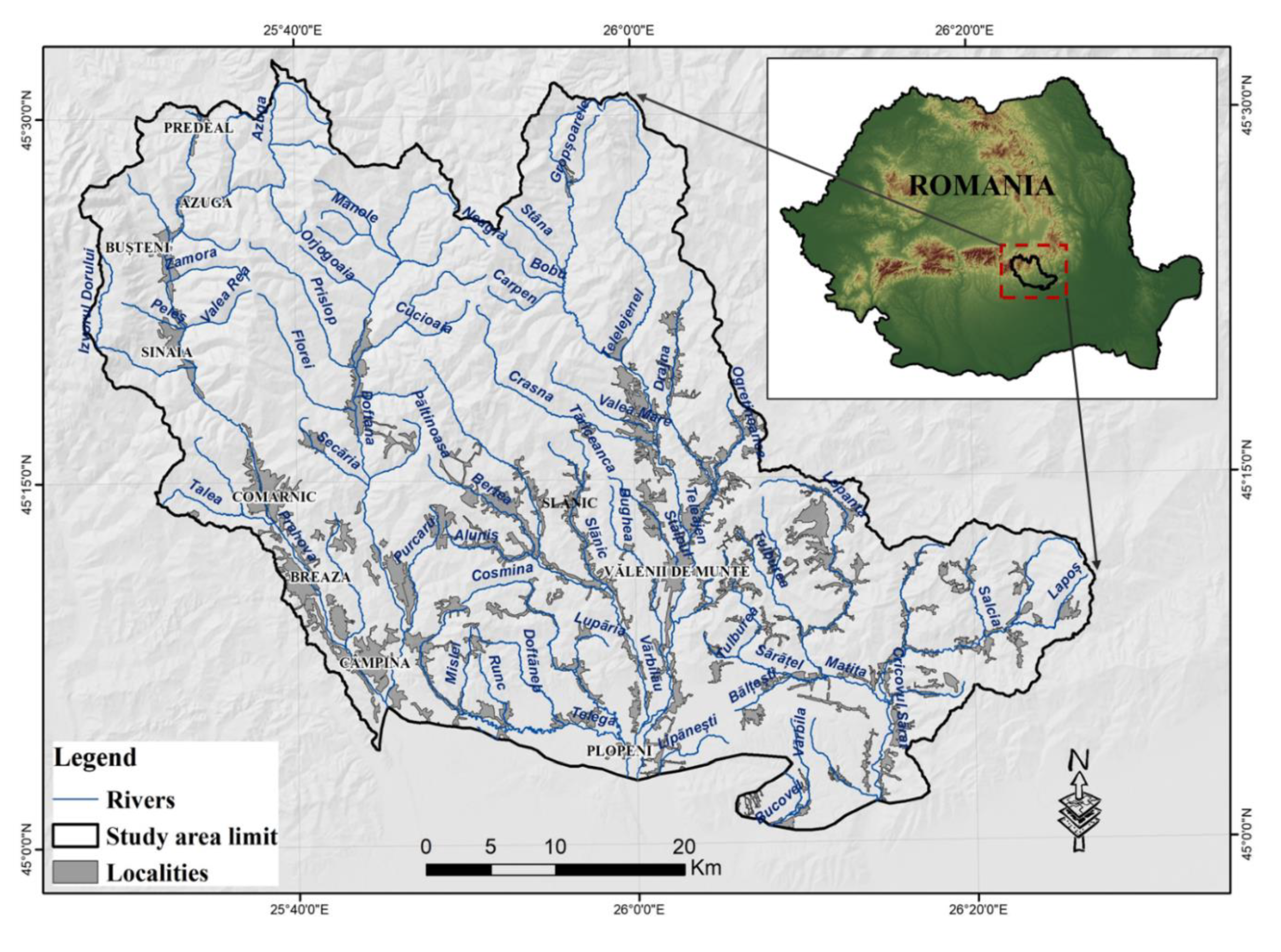
The study area is a catchment of the Prahova river in southeastern Romania and has the following geographical limits: 45°32′21.85″ and 45°00′23.33″ North latitude, and 25°27′32.00″ and 26° 27′10.19″. East longitude (Figure 2). The research area has a total surface of 2600 sq. km.
The relief of the study area that belongs to both the mountain and hilly regions of Carpathian Curvature is developed on a complex lithological structure consisting of loess, gravels, and hard rocks. Most of the hard rocks are specific to areas with slope values over 15°, where the surface runoff is intensified. Overall, at the level of the research zone, there is an altitude difference of almost 2400 m, the highest peaks being located at over 2500 m.
The enormous amount of precipitation, which exceeds 1000 mm annually, falls into the Carpathian region, where the heavy rainfalls leading to flash-floods are frequent. These phenomena occur primarily during the summer, once with the development of convective cloud systems. Land use is another essential factor that controls surface runoff. The built-up surfaces that highly favor the flash-flood potential cover around 10% of the study zone, while the natural grasslands, which also determine a high value of flash-flood potential, have a percentage equal to 15% of the total. The forest surfaces greatly influence the water balance at the river catchment level. From this point of view, a percentage of 52% of the research surface is occupied by forests. It should be mentioned that within the research area are located the most important touristic cities of Romania that are internationally recognized: Predeal, Bușteni, Azuga, and Sinaia.
3.2. Data Used
3.2.1. Flash-Flood Inventory
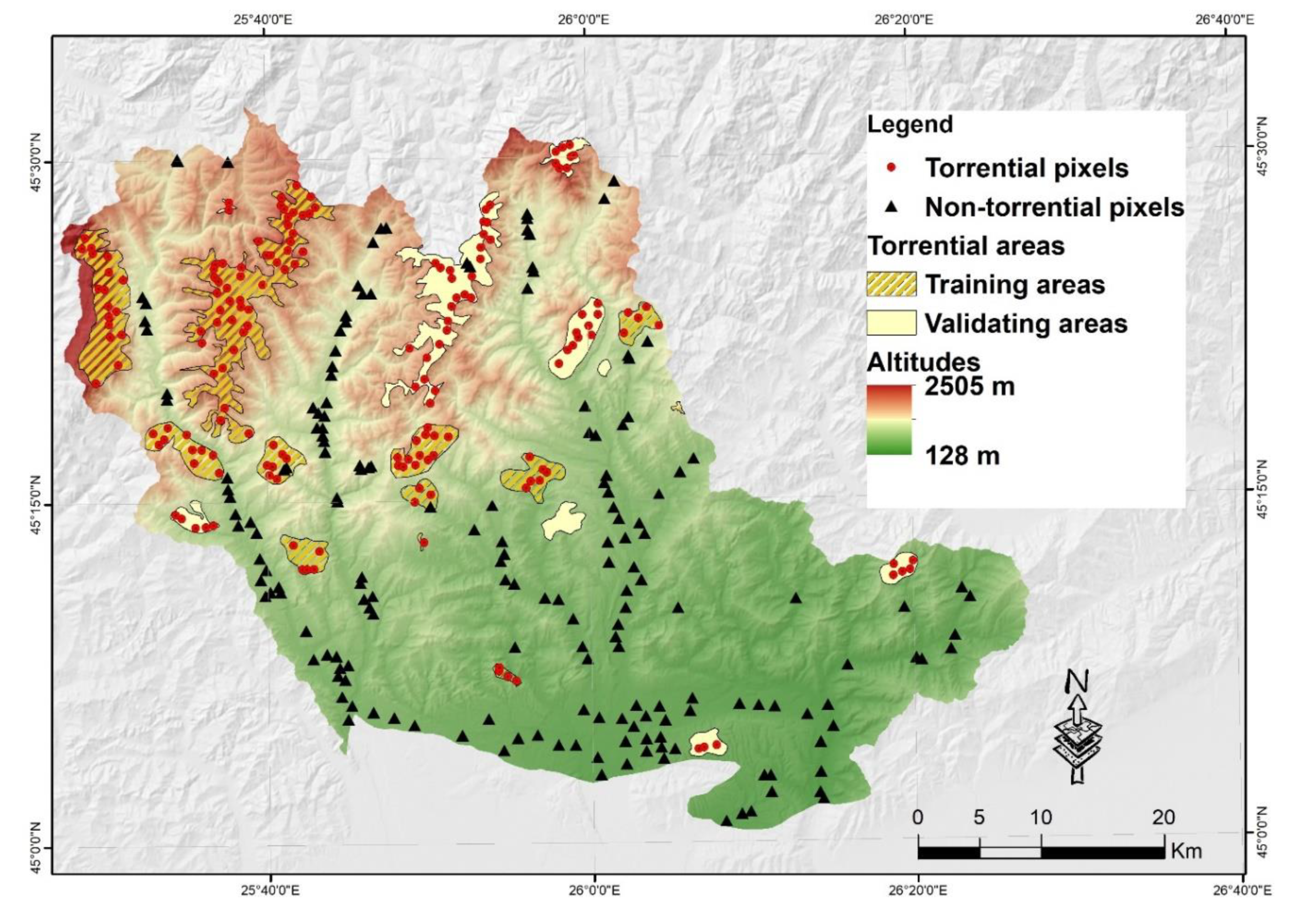
For a more accurate prediction of areas that may be affected in the future by flash-flood, it is essential to correctly evaluate the spatial relationships between the predictors and this phenomenon [50]. In this respect, the areas previously affected by torrential phenomena were identified and mapped. According to Costache and Zaharia (2017) [21], the surfaces characterized by unitary distribution guiles and ravines, which are considered torrential microforms, were considered into the analysis. The remote sensing imagery is essential in order to detect the phenomena from the earth’s surface [51]. It should be noted that these areas were extracted, in a first stage, from Google Earth aerial imagery. It is remarkable, also, that the Google Earth uses aerial imagery, in natural colors, provided by Airbus Defense and Space under contract with French Centre National d’Études Spatiales (CNES) at a spatial resolution of 0.5 m [52]. The surfaces were then validated by field measurements using a Trimble GeoXH 2008 Series GPS device. Finally, a total area of 260 sq. Km, containing about 288,120 pixels, was delineated (Figure 3). In order to be involved in the training process, the geo-environmental values of the torrential areas were generated into a sample, including 178 points. In the GIS environment, these points selected from torrential areas were converted in torrential pixels with the cell size equal to that of the raster of the flash-flood conditioning factors.
3.2.2. Flash-Flood Predictors
Similarly to any other natural risk phenomena, the occurrence process of flash-floods is controlled by the simultaneous action of several geographic factors. The genesis of these natural hazards is related to massive rainfall events. Regarding the study area, the heavy rainfall with the same intensity could occur in any part of its, so it is impossible to differentiate the areas according to this climatic parameter. For this reason, the rainfall factor will be considered constant across the study area, so its values will not be considered within the analysis. Instead, the within the analysis will be involved a number of 10 geographic factors that, with a variable influence, on surface runoff manifestation.
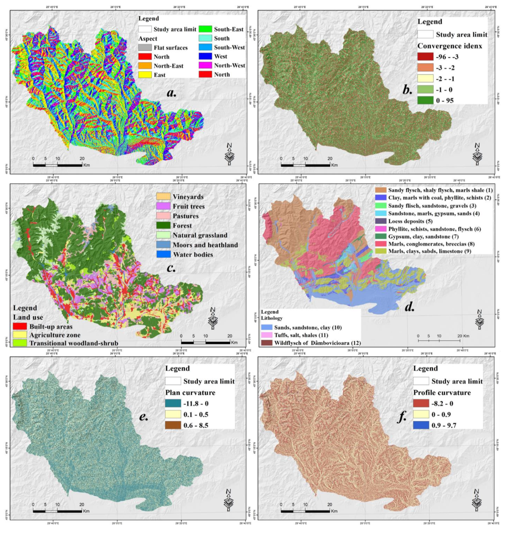
Lithology is a crucial flash-flood predictor because it controls the water infiltration process during the massive rainfall events. Thus, the hard rocks with a high impermeability degree will favor the surface runoff manifestation, unlike sedimentary rocks, that favor the infiltration process. From the Geological Map of Romania, 1:200,000, a number of 12 lithological groups were extracted across the study area. Obtained initially in vector format, they were transformed to grid dataset with a size of cell equal to 30 m (Figure 4d).
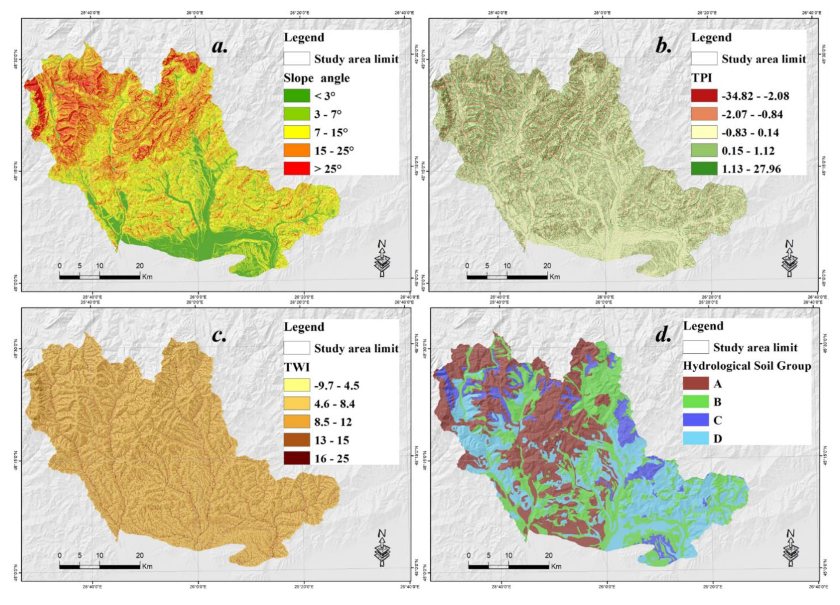
Hydrological Soil Group also influences the quantity of water infiltrated into the soil, the hydraulic conductivity ranging from 1 µm/s (group D) to more than 40 µm/s (group A). The hydrological soil group A occurs on most of the surface area (801 sq. km), followed by group B (727 sq. km), group C (213 sq. km) and group D (682 sq. km) (Figure 5d). Initially extracted in vector format, by using the Digital Soils Map of Romania, 1:200,000, this layer was transformed into a grid dataset with a size of cell equal to 30 m.
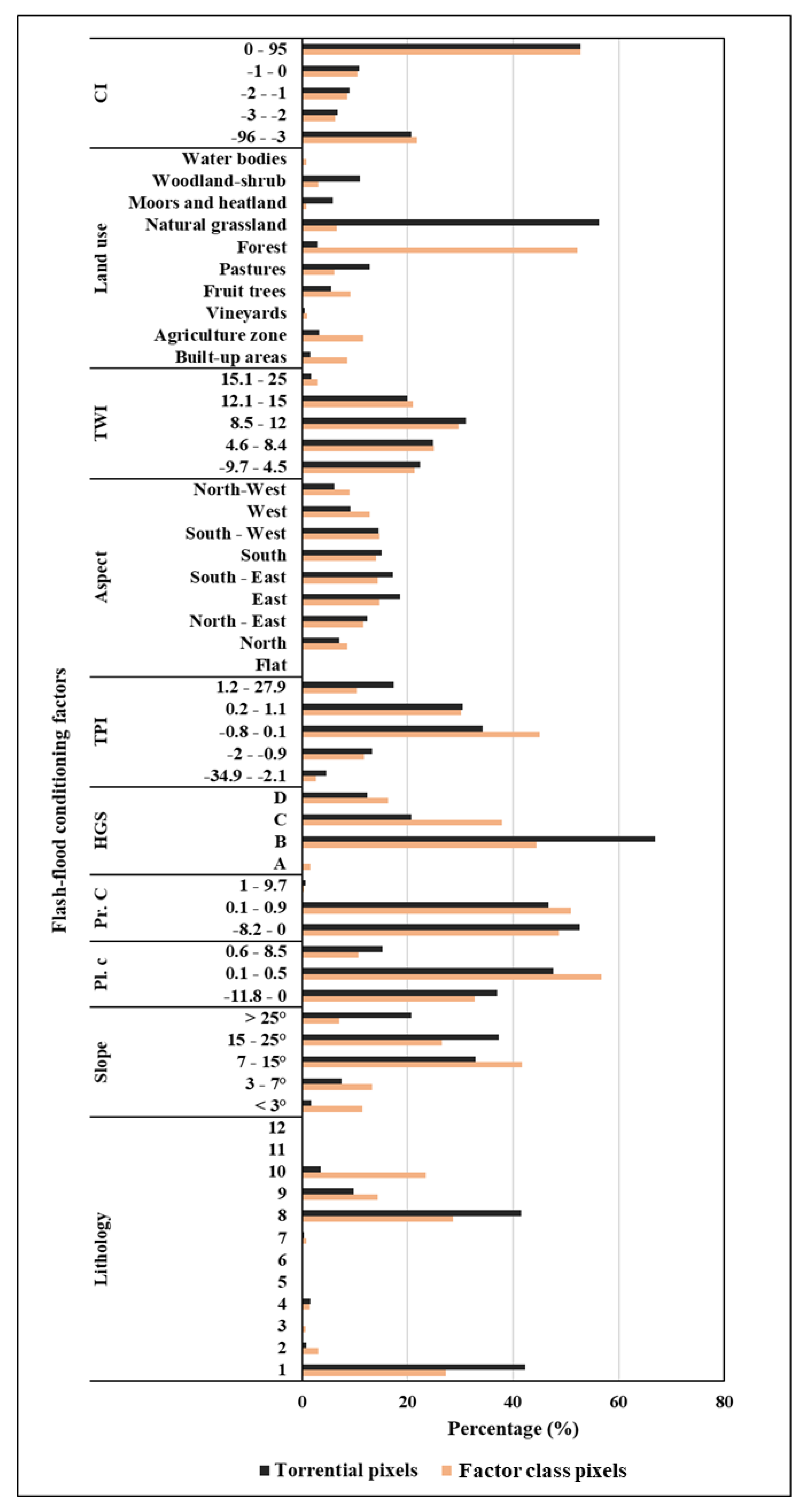
Land use, together with the slope angle, controls the surface runoff velocity by influencing the Manning Roughness coefficients and by influencing the rainfall interception process [53,54,55,56]. Forest areas are characterized by high values for both rainfall interception and Manning Roughness coefficients. Therefore, these land-use types are the most restrictive for surface runoff while the built-up areas and pastures favor the flash-flood occurrence. Within the study were identified a number of 10 land use categories (Figure 4c), the most extensive surfaces being covered by forests (50%), while the most torrential areas are located within the natural grasslands category (55%).
Slope angle has been confirmed as a key factor for flash-flood studies because it greatly controls the speed of the floodwaters [57,58,59,60]. This was derived from the Digital Elevation Model (DEM) with a cell size of 30 m. The DEM was extracted from Shuttle Radar Topography Mission (SRTM) database at a spatial resolution of 30 m. It should be noted that SRTM is an international project coordinated by the U.S. National Geospatial-Intelligence Agency (NGA) and the U.S. Aeronautics and Space Administration (NASA) [61]. According to Zaharia et al. [62] the following slope classes have been established: 0°–3°, 3°–7°, 7°–15°, 15°–25° and >25° (Figure 5a). It is remarkable the fact that the most torrential areas are included in the class ranging from 15° to 25°, while the maximum concentration of torrential pixels is present within the class characterized by slopes above 25°. This spatial distribution of torrential areas shows that the flash-flood potential increases with the increase of slope value.
Convergence index (Ci) is a morphometric factor with high importance on the flash-flood potential [18,21]. Its negative values highlight the river valleys perimeters, meanwhile the values higher than 0 highlight the presence of the interfluvial areas. For Ci computation, the Digital Elevation Model was imported into SAGA GIS 2.1.0 software. The next 5 classes were established for the values of Ci: (−96)–(−3), (−3)–(−2), (−2)–(−1), (−1)–0 and 0–95 (Figure 4b).
Profile curvature was taken into account because it is useful to delimit the areas characterized by high runoff and the areas with low runoff [17]. The surfaces with accelerated runoff (−8.2–0) occupy approximately 50% of the total (Figure 5f), is also characterized by the presence of 50% of torrential pixels (Figure 6).
Plan curvature allows us to distinguish between the areas on which the convergent runoff occurs and the areas on which the divergent runoff occurs. Therefore, we can state that this morphometric factor controls the water flow (Pham et al., 2017). Values between 0.1 and 0.5 are spread on almost 58% of the research area and incorporate 48% of the torrential pixels (Figure 5e).
Topographic Position Index (TPI) is another morphometric factor which was obtained in SAGA GIS software. It is defined as the difference between each cell of the Digital Elevation Model and the mean elevation of a defined neighborhood around that cell [63]. The TPI can be calculated according to the following formulas:
where is the elevation of the central cell for which the TPI is calculated, is the average elevation around the central cell within a specific radius (R) [64].
The Natural Breaks method was used to divide the TPI value into 5 groups. These groups were finally used to generate the TPI map. Thus, the largest surface is covered with the third TPI values class (45%), ranging from (−0.83) to 0.14 (Figure 5b). The same class is characterized by the largest surface of torrential areas, which counts around 34% of the total number of torrential pixels.
Topographic Wetness Index (TWI) is defined as a quantitative index that indicates the balance between the flow accumulation and the drainage conditions existent at the local scale [65]. TWI is a widely used conditioning factor in the delineation of flood-prone areas [66]. This another essential runoff factor can be calculated through the following relation [67]:
where α represents the upslope area that drains through a pixel and tan β represents the slope angle in that pixel.
Similar to TPI, the TWI values, ranging between −9.7 and 25 (Figure 5c), were classified by the mean of the Natural Breaks algorithm. Therefore, five classes were used in order to map the TWI values. The medium TWI values (8.5–12) cover the highest percentage of the study area (29%) (Figure 6).
Aspect is a predictor obtained from the Digital Elevation Model. This morphometric indicator was split into 10 groups, which influence in a different manner the soil humidity, solar radiation, or the amount and regime of rainfall. With a weight of 15% of the study area, eastern and south-western surfaces rank the first in terms of area occupied by each aspect direction (Figure 4a). Eastern surfaces contain around 18.3% of the total torrential pixels (Figure 6).
4. Proposed Ensemble Approach Based on DNN, AHP, and FR for Flash-Flood Susceptibility Mapping
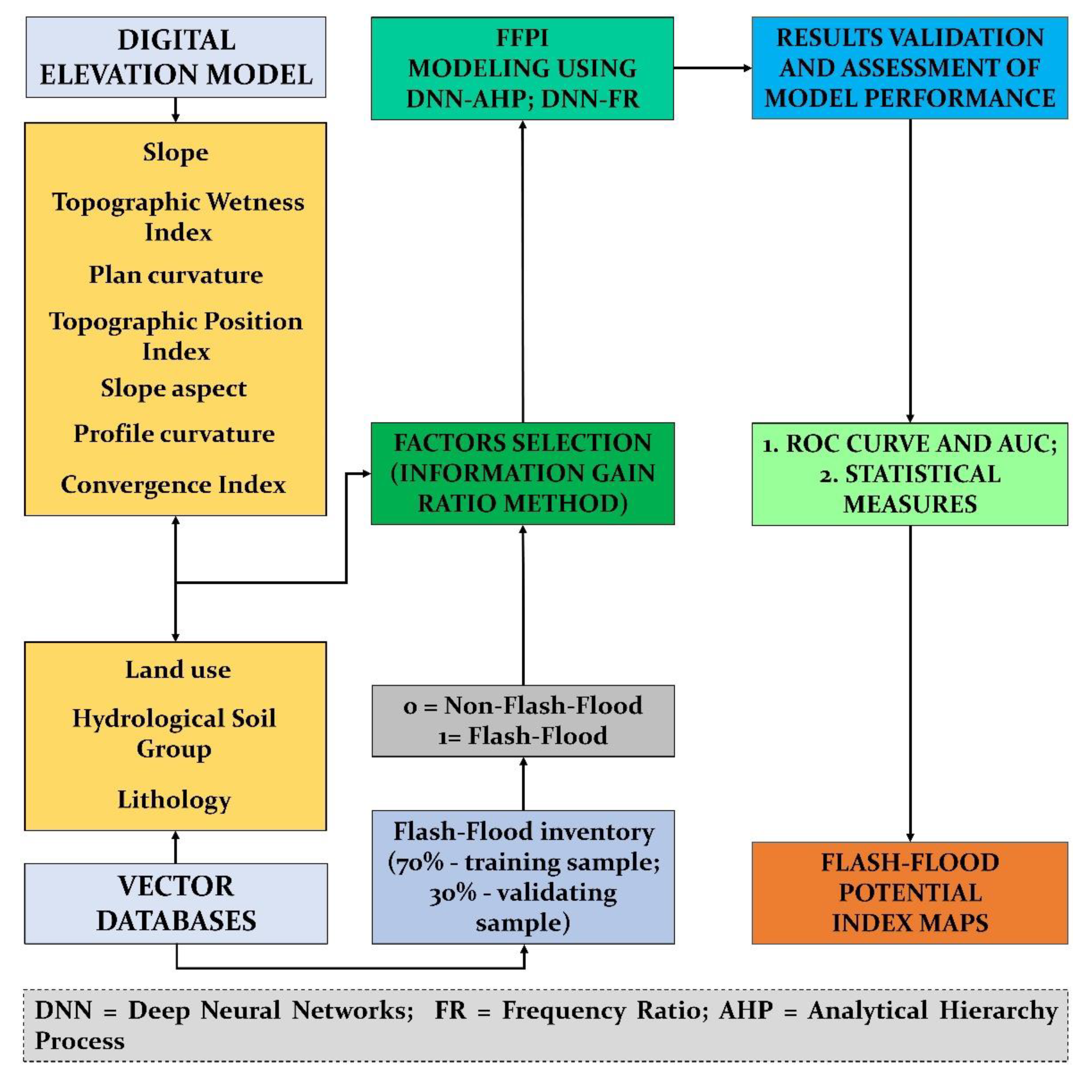
Because the main objective of this research is the mapping of surfaces prone flash-floods, only the geospatial data will be used in the analysis. The entire workflow of the analysis is synthetically presented in Figure 7.
4.1. Flood Database
The flood databases, containing 10 flash-flood predictors and 178 flash-flood locations, were processed and created in ArcGIS 10.5 software (ESRI, Redlands, CA, USA). According to the literature, the selection and the inclusion into the analysis of another sample containing the locations where the phenomenon is absent are mandatory in order to increase the performance of the models [24,49,68]. Therefore, another 178 non-torrential points were located over the areas having a slope around 0° where flash-floods are almost impossible. According to the vast majority of researchers, 70% of the torrential and non-torrential pixels were considered as training data set, while the rest of 30% will be employed to validate the results of applied models [2,47,50,69]. All the data involved in the methodological process is transformed into a raster data set with a cell dimension of 30 × 30 m.
4.2. Data Diagnosis and Checking
Using the Information Gain Ratio (IGR), the predictors were selected according to their predictive power. The IGR is one of the most popular methods intended to check the predictive ability of a predictor in terms of a given phenomenon [70]. This algorithm, proposed by Chapi et al. [10] uses the following relation:
where D is the training dataset composed of n input samples, n (Yi, D) is the number of samples in the training data D belonging to the class label Yi (Torrential, non-Torrential).
4.3. Model Setup and Training
A number of 10 pair-wise comparison matrices were constructed in Excel 2016 software (Microsoft, Redmond, WA, USA)for the derivation of AHP weights corresponding to each factor class/category. The consistency of each matrix was evaluated by calculating the Consistency Ratio according to 2.2.
The computation of FR coefficients required the use of both ArcGIS 10.5 and Excel 2016 software. In the first stage, in a GIS environment, the information regarding the values of predictors was extracted to each flash-flood location. Further, this information was used in Excel, where the FR coefficients were calculated using formula (13). The FR coefficients were normalized in the range 0.1–0.9 through the following equation [27]:
where y is the standardized value of x; x is the current value of the variable; d is the range value limits and n is is standardization range limits.
The values of AHP weights and FR coefficients were further used to compute the ensemble models DNN-AHP and DNN-FR. Using these ensembles, the FFPI values were determined across the study area. It should be mentioned that the DNN-AHP and DNN-FR hybrid models were trained by using the Adam method, which classified the raster pixels into the following two categories flash-flood and non-flash-flood. According to Figure 1, the architecture of DNN ensembles is characterized by a number of 3 hidden layers. Each of them contains 100 neurons. A trial-error procedure was employed to establish the numbers of hidden neurons and hidden layers.
4.4. Quality Evaluation
In a first step, the results quality was checked by computing the next statistical metrics: Negative Predicted Values (NPV), Positive Predictive Value (PPV), Specificity, Sensitivity, Accuracy, Kappa Index. In order to determine the values of these statistical indices, the true positive (TP), the false positive (FP), the false negative (FN), and the true negative (TN) were involved in the following formulas:
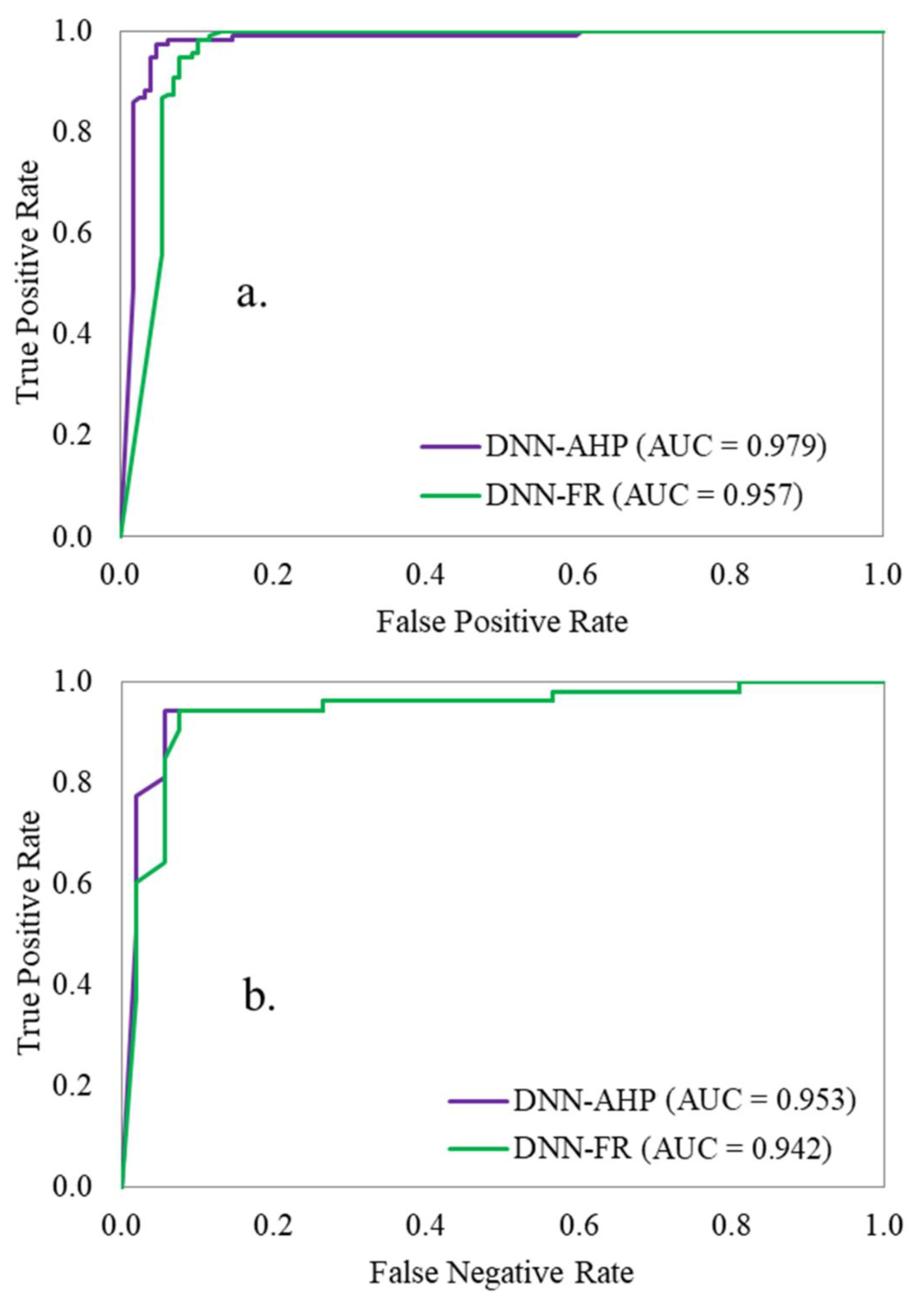
The results of DNN ensembles were also evaluated by using the Receiver Operating Characteristic (ROC) Curve. This algorithm is frequently used to evaluate the reliability of results provided by a model [10,23,71,72]. To draw the ROC Curve, the acquired results and existing flash-flood locations were compared. Therefore, the FFPI results were tested using the success rate, obtained with the training sample, and also the prediction rate, constructed with the validation sample. The Area Under Curve (AUC) associated with the success rate shows the model’s performance in terms of results classification, while the prediction rate highlights the accuracy of the results. An AUC value near 1 indicates a high performant model, while a non-informative model is revealed by an AUC near 0 [8,21]. The AUC can be estimated using Equation (21) below [70]:
where TP (true positive) is the sum of flash-flood pixels accurately classified, TN (true negative) is the sum of non-flash-flood pixels accurately classified, P and N are the sum of flash-flood pixels and non-flash-flood pixels, respectively.
4.5. Compiling Flash-Flood Susceptibility Map
The derivation of the importance assigned to each flash-flood predictor was possible by applying the DNN-AHP and DNN-FR. The last step of flash-flood potential mapping was performed in ArcGIS 10.5, where the weights of predictors were multiplied with the FR and AHP coefficients.
5. Results and Analysis
5.1. Predictive Capability of Flash-Flood Predictors
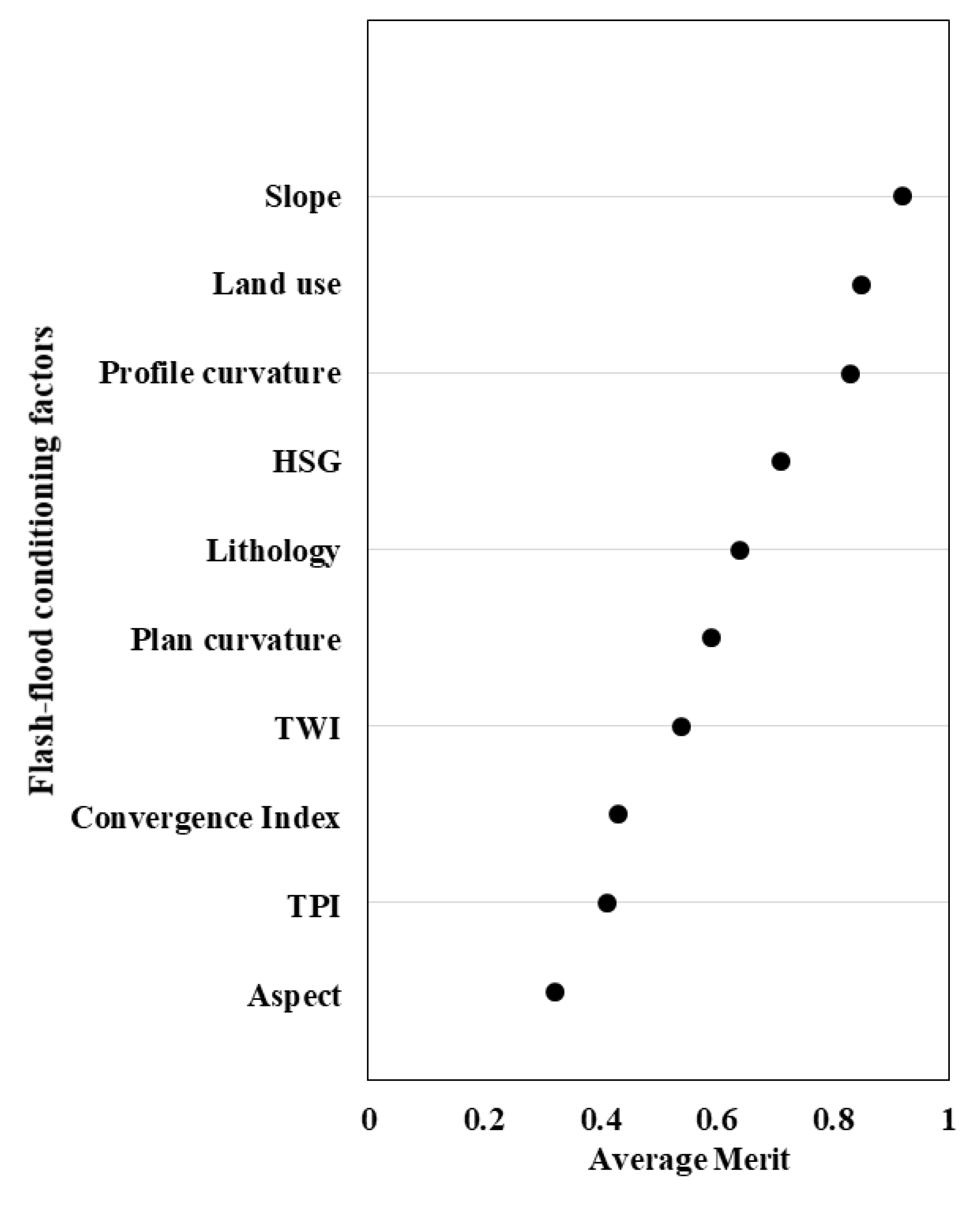
Figure 8 shows the results regarding the predictive capability of flash-flood predictors which were estimated through the Information Gain Ratio method. The highest predictive capability was attributed to slope angle (0.92), followed by profile curvature (0.83), hydrological soil group (0.71), lithology (0.64), plan curvature (0.59), TWI (0.54), convergence index (0.43), TPI (0.41) and aspect (0.32). As can be seen, the weak predictive capability, which is equal to 0.32, is higher than 0 and, therefore, all the predictors initially considered were used in the present analysis.
5.2. AHP and FR Weights
All the possible comparison, involving the factor classes/categories, are included in Table 1. In this regard, by attributing the relative dominant value, each class/category was rated against every other. Table 1 also includes the final coefficients resulted from the application of the AHP algorithm. As was mentioned in Section 4.3, in order to evaluate the consistency of judgments, the CR value for each matrix was computed. Because all CR values are below 0, we can state that all the comparisons included in the matrices are consistent. Moreover, the other parameters used in the AHP algorithm workflow are shown in Table 2.
Together with AHP normalized values, Table 1 also includes the normalized value of FR coefficients. Within each flash-flood predictor, the highest FR normalized values (0.9) were obtained by the following classes/categories: slope angles above 25°, TPI ranging from −20 to −3.8, TWI ranging from −9 to 4.5, grassland land use category, sandy flysch lithological group, profile curvature ranging from 0.9 to 9.7, plan curvature ranging from 0.6 to 8.5, eastern slopes, hydrological soil group B and convergence index ranging from −2 to −1.
5.3. Flash-Flood Modelling with DNN-AHP and DNN-FR
The training process of DNN-AHP and DNN-FR was ensured by the use 249 flash-flood and non-flash-flood locations, which account around 70% of the entire dataset. Together with the information regarding the presence or the absence of flash-flood past phenomena, to these points were attributed the AHP and FR weights. In terms of DNN-AHP ensemble, its training performance is highlighted by the values of the following metrics: PPV = 95.2%, NPV = 100%, Sensitivity = 100%, Specificity = 95.42%, Accuracy = 97.6%, Kappa = 0.952 (Table 3). In the training process the DNN-FR ensemble achieved also high performances that are denoted by the following values: PPV = 100%, NPV = 99.2%, Sensitivity = 99.21%, Specificity = 100%, Accuracy = 99.6%, Kappa = 0.992. The use of the other 30% of the dataset included in the validating sample revealed the following values for DNN-AHP: PPV = 92.5%, NPV = 100%, Sensitivity = 100%, Specificity = 93%, Accuracy = 96.23% and Kappa = 0.925. The prediction data used in the case of DNN-FR led to the achievement of the next values: PPV = 100%, NPV = 98.08, Sensitivity = 98.15, Specificity = 99.05%, Kappa = 0.981. The ROC Curve along with its associated AUC were also involved in the evaluation of the models performances.
The use of ROC Curve confirms the outstanding performances achieved by DNN-AHP and DNN-FR ensembles. Thus, in terms of Success Rate, the AUC value of the DNN-AHP ensemble was equal to 0.979, while the DNN-FR obtained an AUC of 0.957 (Figure 9a). The use of the Prediction Rate revealed an AUC of 0.953 for DNN-AHP, while the AUC of DNN-FR was equal to 0.942 (Figure 9b).
Given the high performances of the two ensembles presented above, the deep learning models were involved in the mapping procedure of FFPI across the study area. This operation was done in ArcGIS 10.5 by using the FFPI values in raster format.
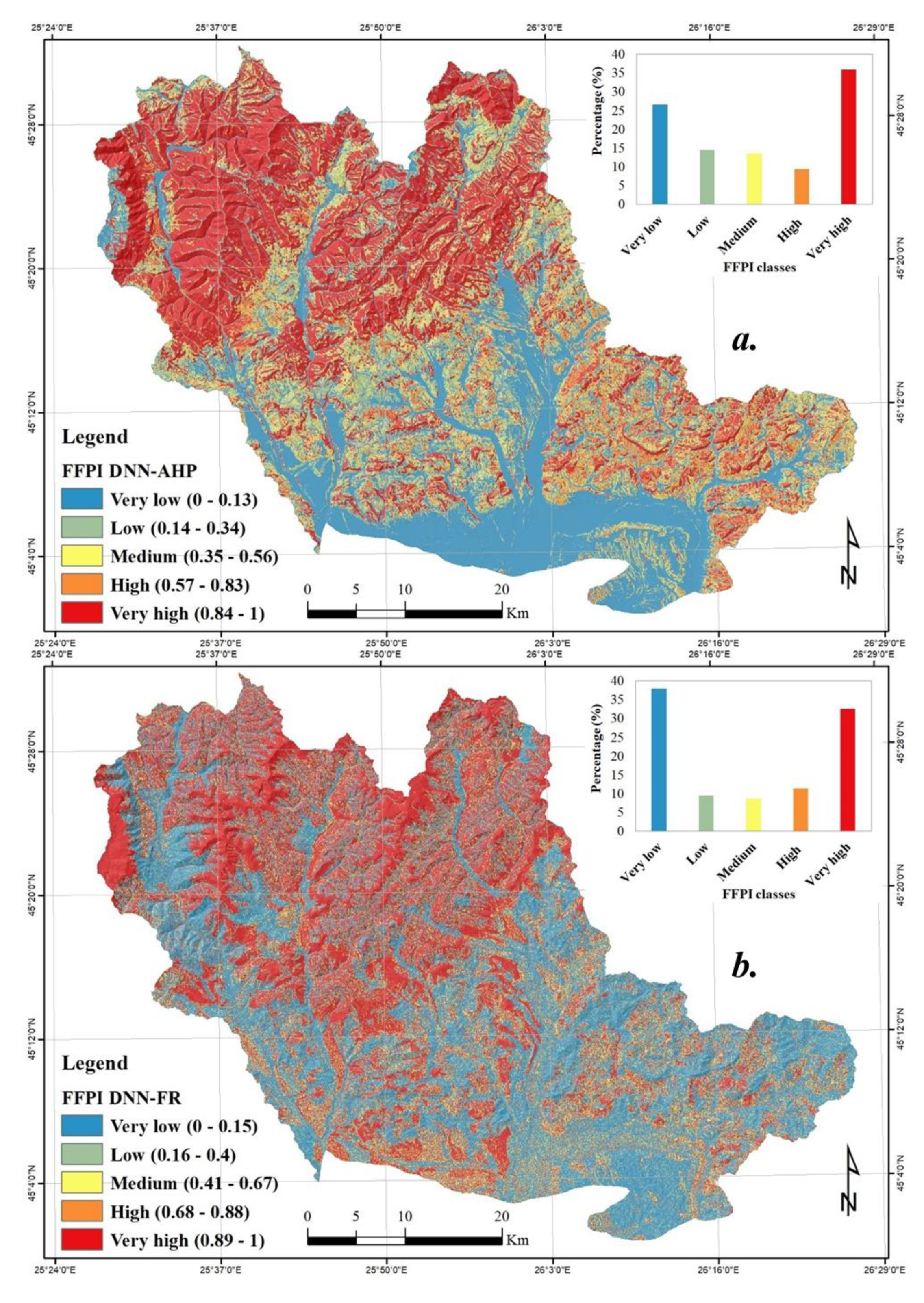
According to Figure 10, the values of both indices, FFPIDNN-AHP and FFPIDNN-FR, were partitioned into 5 classes by using the Natural Breaks algorithm. In terms of FFPIDNN-AHP, the very low values ranging from 0 to 0.13 cover around 37.9% of the study area, while the low values between 0.14 and 0.34 quantify approximately 9.48% of the research zone. The medium FFPIDNN-AHP class is present on 8.69% of the research zone, while the high and very high classes span on a total of 43.9% of the study area (Figure 10a). In terms of FFPIDNN-FR, it can be observed that the first and the second classes, between 0 and 0.4, quantify approximately 41% of the entire study zone, while the medium class accounts for 13.58% of the total surface. The regions with critical FFPIDNN-FR values are distributed over 45% of the research territory (Figure 10b).
6. Discussions
In Romania, a significant increase in the intensity of flash-floods can be observed in recent years [24]. This fact is mainly associated with global climate change affecting the area in which Romania is located but also is due to the transformations undergone within the land-use, especially the excessive deforestation. [21]. The most affected area by these natural risk phenomena is the mountain and hilly area of Romania, where the slope of the relief, and the lack of forest across certain regions, create the premises for the production of devastating fast-floods. [18]. This is also the case of the Prahova river basin area on which the present research work has focused. Thus, at the level of the study area, there is a need to identify as accurately as possible the perimeters exposed to the formation of the torrential flow which further causes the production of severe flash-floods. Testing of many modern methods for detecting these surfaces is mandatory in order to identify the techniques that provide the best results and which can be recommended to be used in other areas exposed to flash-floods. The potential for rapid surface runoff at the level of the Prahova River basin has been determined in the past through bivariate statistical techniques combined with machine learning algorithms such as Logistic Regression, Rotation Forest, Multilayer Perceptron Neural Network, Support Vector Machine, Naive Bayes, k Nearest Neighbor (k-NN) or K-Star [25,26,28,73]. All these models have achieved high performances and are generally characterized by accuracies that exceeded 85%. The AHP model has been applied, within the same study area, in combination with k-NN and K-Star, obtaining also high accuracy values (90.1%) [73]. In this study, instead, it was decided to use DNN which is considered one of the state of the art techniques used to determine the susceptibility to this type of hazard [74]. In order to increase the performance of the model, the input data were optimized by determining the AHP and FR weights for each class/category of factors. The high performance of DNN-FR and DNN-AHP algorithms was also demonstrated in the present study in which the accuracy of the models was very close to perfection (higher than 94%). Thus, their accuracy exceeded the accuracy of the best model applied in previous research, in the same study area, namely Rotation Forest (RF) (91%). The RF algorithm was applied by Costache [26]. The application of the AHP method in other studies regarding the evaluation of the susceptibility to floods and flash-floods in other regions is also noted. One such example is the study carried out by Das [66], which evaluated the Ulhas basin (India) from the flood susceptibility point of view using the AHP method. It should be mentioned that the accuracy of stand-alone AHP method (84%), applied by Das [75], was lower than the accuracy of DNN-AHP (97.9%) obtained in the present research.
According to Figure 8, the factor with the highest influence on flash-flood susceptibility is the slope angle. Land use and profile curvature also have an essential influence in the flash-flood triggering. The high slopes and the absence of forests in the northern and north-western part of the study area is the main explanation for the very high FFPI values recorded within these regions. As can be observed in Figure 10 the most susceptible areas are especially located in the aforementioned areas are represented with red color, because this color is usually used to highlight the high intensity of a phenomenon.
7. Conclusions
Identifying, as accurately as possible, the areas with a high surface runoff potential is a necessary action based on which the non-structural measure for defense against the flash-flood adverse effects can be adopted. Given this consideration, the present study proposes a novel methodology used to identify the areas exposed to flash-flood occurrence across the Prahova river basin. The main goal of the developed workflow was of the computation of the Flash-Flood Potential Index through two ensembles of DeepNeural Networks (DNN-AHP and DNN-FR). A number of 10 predictors, selected through the Information Gain Ration method, along with 70% of flash-flood and non-flash-flood samples, were employed in the training procedure of the models, while the validation of the results was carried out by using the other 30% of the data sample. The assessment of the performance of the models and the validation of the result was made in two steps: (i) through ROC Curve and (ii) by calculating several statistical metrics. ROC Curve method revealed that the most reliable ensemble model was DNN-AHP taking into account both Success Rate (AUC = 0.979) and Prediction Rate (AUC = 0.953). Areas identified as having critical values (high and very high) of flash-flood potential cover between 43.9% (FFPIDNN-AHP) and 45% (FFPIAHP) of the study area. These areas are distributed mainly in the North-Western part where several touristic cities are located. In these conditions, these localities are highly vulnerable to flash-flood phenomena. Many flash-flood events occurred during the next years: 2005, 2006, 2010, 2014, 2017, and 2018.
The principal novelty that characterizes the present study consists of the use for the first time in the literature of the DNN-AHP and DNN-FR ensembles models to assess the susceptibility to natural risk phenomena, and therefore for estimating the Flash-Flood Potential Index across the study area. The outcomes of the present research can be successfully used for effective territorial planning as well as for the improvement of flash-flood forecasts and warning accuracy.
Author Contributions
Conceptualization, R.C. and D.T.B.; Data curation, R.C. and D.T.B. Methodology, R.C., P.T.T.N. and D.T.B. Writing—original draft, R.C. and D.T.B.; Writing—review and editing, R.C., P.T.T.N., and D.T.B. All authors have read and agreed to the published version of the manuscript.
Funding
This research was supported by Research Institute of the University of Bucharest (Romania) and partially supported by University of South-Eastern Norway (Norway), and Institute of Research and Development, Duy Tan University (Vietnam).
Conflicts of Interest
The authors declare no conflict of interest.
References
- Khosravi, K.; Pourghasemi, H.R.; Chapi, K.; Bahri, M. Flash flood susceptibility analysis and its mapping using different bivariate models in Iran: A comparison between Shannon’s entropy, statistical index, and weighting factor models. Environ. Monit. Assess. 2016, 188, 656. [Google Scholar] [CrossRef]
- Costache, R.; Pravalie, R.; Mitof, I.; Popescu, C. Flood vulnerability assessment in the low sector of Saratel Catchment. Case study: Joseni Village. Carpathian J. Earth Environ. Sci. 2015, 10, 161–169. [Google Scholar]
- Gashaw, W.; Legesse, D. Flood hazard and risk assessment using GIS and remote sensing in Fogera Woreda, Northwest Ethiopia. In Nile River Basin; Springer: Berlin/Heidelberg, Germany, 2011; pp. 179–206. [Google Scholar]
- Khosravi, K.; Pham, B.T.; Chapi, K.; Shirzadi, A.; Shahabi, H.; Revhaug, I.; Prakash, I.; Bui, D.T. A comparative assessment of decision trees algorithms for flash flood susceptibility modeling at Haraz watershed, northern Iran. Sci. Total Environ. 2018, 627, 744–755. [Google Scholar] [CrossRef] [PubMed]
- Sarhadi, A.; Soltani, S.; Modarres, R. Probabilistic flood inundation mapping of ungauged rivers: Linking GIS techniques and frequency analysis. J. Hydrol. 2012, 458, 68–86. [Google Scholar] [CrossRef]
- Cao, C.; Xu, P.; Wang, Y.; Chen, J.; Zheng, L.; Niu, C. Flash flood hazard susceptibility mapping using frequency ratio and statistical index methods in coalmine subsidence areas. Sustainability 2016, 8, 948. [Google Scholar] [CrossRef] [Green Version]
- Casale, R.; Margottini, C. Floods and Landslides: Integrated Risk Assessment: Integrated Risk Assessment; with 30 Tables; Springer Science & Business Media: Berlin, Germany, 1999; ISBN 3-540-64981-6. [Google Scholar]
- Youssef, A.M.; Pradhan, B.; Hassan, A.M. Flash flood risk estimation along the St. Katherine road, southern Sinai, Egypt using GIS based morphometry and satellite imagery. Environ. Earth Sci. 2011, 62, 611–623. [Google Scholar] [CrossRef]
- Bubeck, P.; Botzen, W.J.; Aerts, J.C. A review of risk perceptions and other factors that influence flood mitigation behavior. Risk Anal. Int. J. 2012, 32, 1481–1495. [Google Scholar] [CrossRef] [PubMed] [Green Version]
- Chapi, K.; Singh, V.P.; Shirzadi, A.; Shahabi, H.; Bui, D.T.; Pham, B.T.; Khosravi, K. A novel hybrid artificial intelligence approach for flood susceptibility assessment. Environ. Model. Softw. 2017, 95, 229–245. [Google Scholar] [CrossRef]
- Li, W.; Lin, K.; Zhao, T.; Lan, T.; Chen, X.; Du, H.; Chen, H. Risk assessment and sensitivity analysis of flash floods in ungauged basins using coupled hydrologic and hydrodynamic models. J. Hydrol. 2019, 572, 108–120. [Google Scholar] [CrossRef]
- Smith, G. Flash flood potential: Determining the hydrologic response of FFMP basins to heavy rain by analyzing their physiographic characteristics. In White Pap. Available NWS Colo. Basin River Forecast Cent. Web Site Httpwww Cbrfc Noaa Govpapersffpwpap Pdf; 2003. Available online: http://www.cbrfc.noaa.gov/papers/ffp_wpap.pdf (accessed on 31 October 2019).
- Brewster, J. Development of the Flash Flood Potential Index (FFPI) for Central NY & Northeast PA. 2010, pp. 2–4. Available online: https://documents.pub/document/development-of-the-flash-flood-potential-ffpi-the-flash-flood-potential-index.html (accessed on 3 November 2019).
- Kruzdlo, R.; Ceru, J. Flash Flood Potential Index for WFO Mount Holly/Philadelphia. 2010, pp. 2–4. Available online: http://bgmresearch.eas.cornell.edu/research/ERFFW/posters/kruzdlo_FlashFloodPotentialIndexforMountHollyHSA.pdf (accessed on 5 November 2019).
- Zogg, J.; Deitsch, K. The Flash Flood Potential Index at WFO Des Moines, Iowa; National Weather Service Working Paper; 2013. Available online: http://www.crh.noaa.gov/images (accessed on 8 November 2019).
- Minea, G. Assessment of the flash flood potential of Bâsca River Catchment (Romania) based on physiographic factors. Open Geosci. 2013, 5, 344–353. [Google Scholar] [CrossRef] [Green Version]
- Zaharia, L.; Minea, G.; Ioana-Toroimac, G.; Barbu, R.; Sârbu, I. Estimation of the areas with accelerated surface runoff in the upper Prahova watershed (Romanian Carpathians). In Proceedings of the International Conference on Water, Climate and Environment, Ohrid, Macedonia, 28 May 2012; pp. 1–10. [Google Scholar]
- Zaharia, L.; Costache, R.; Prăvălie, R.; Ioana-Toroimac, G. Mapping flood and flooding potential indices: A methodological approach to identifying areas susceptible to flood and flooding risk. Case study: The Prahova catchment (Romania). Front. Earth Sci. 2017, 11, 229–247. [Google Scholar] [CrossRef]
- Tincu, R.; Lazar, G.; Lazar, I. Modified flash flood potential index in order to estimate areas with predisposition to water accumulation. Open Geosci. 2018, 10, 593–606. [Google Scholar] [CrossRef]
- Romulus, C.; Iulia, F.; Ema, C. Assessment of surface runoff depth changes in Sǎrǎţel River basin, Romania using GIS techniques. Open Geosci. 2014, 6, 363–372. [Google Scholar] [CrossRef]
- Costache, R.; Zaharia, L. Flash-flood potential assessment and mapping by integrating the weights-of-evidence and frequency ratio statistical methods in GIS environment–case study: Bâsca Chiojdului River catchment (Romania). J. Earth Syst. Sci. 2017, 126, 59. [Google Scholar] [CrossRef]
- Tehrany, M.S.; Pradhan, B.; Jebur, M.N. Flood susceptibility mapping using a novel ensemble weights-of-evidence and support vector machine models in GIS. J. Hydrol. 2014, 512, 332–343. [Google Scholar] [CrossRef]
- Hong, H.; Tsangaratos, P.; Ilia, I.; Liu, J.; Zhu, A.-X.; Chen, W. Application of fuzzy weight of evidence and data mining techniques in construction of flood susceptibility map of Poyang County, China. Sci. Total Environ. 2018, 625, 575–588. [Google Scholar] [CrossRef]
- Costache, R. Flood Susceptibility Assessment by Using Bivariate Statistics and Machine Learning Models-A Useful Tool for Flood Risk Management. Water Resour. Manag. 2019, 33, 3239–3256. [Google Scholar] [CrossRef]
- Costache, R. Flash-Flood Potential assessment in the upper and middle sector of Prahova river catchment (Romania). A comparative approach between four hybrid models. Sci. Total Environ. 2019, 659, 1115–1134. [Google Scholar] [CrossRef]
- Costache, R. Flash-flood Potential Index mapping using weights of evidence, decision Trees models and their novel hybrid integration. Stoch. Environ. Res. Risk Assess. 2019, 33, 1375–1402. [Google Scholar] [CrossRef]
- Costache, R.; Bui, D.T. Spatial prediction of flood potential using new ensembles of bivariate statistics and artificial intelligence: A case study at the Putna river catchment of Romania. Sci. Total Environ. 2019, 691, 1098–1118. [Google Scholar] [CrossRef]
- Costache, R.; Hong, H.; Wang, Y. Identification of torrential valleys using GIS and a novel hybrid integration of artificial intelligence, machine learning and bivariate statistics. Catena 2019, 183, 104179. [Google Scholar] [CrossRef]
- Rahman, M.; Ningsheng, C.; Islam, M.M.; Dewan, A.; Iqbal, J.; Washakh, R.M.A.; Shufeng, T. Flood Susceptibility Assessment in Bangladesh Using Machine Learning and Multi-criteria Decision Analysis. Earth Syst. Environ. 2019, 3, 585–601. [Google Scholar] [CrossRef]
- Althuwaynee, O.F.; Pradhan, B.; Park, H.-J.; Lee, J.H. A novel ensemble bivariate statistical evidential belief function with knowledge-based analytical hierarchy process and multivariate statistical logistic regression for landslide susceptibility mapping. Catena 2014, 114, 21–36. [Google Scholar] [CrossRef]
- Dahri, N.; Abida, H. Monte Carlo simulation-aided analytical hierarchy process (AHP) for flood susceptibility mapping in Gabes Basin (southeastern Tunisia). Environ. Earth Sci. 2017, 76, 302. [Google Scholar] [CrossRef]
- Papaioannou, G.; Vasiliades, L.; Loukas, A. Multi-criteria analysis framework for potential flood prone areas mapping. Water Resour. Manag. 2015, 29, 399–418. [Google Scholar] [CrossRef]
- Nielsen, M.A. Neural Networks and Deep Learning; Determination Press: San Francisco, CA, USA, 2015; Volume 25. [Google Scholar]
- Schmidhuber, J. Deep learning in neural networks: An overview. Neural Netw. 2015, 61, 85–117. [Google Scholar] [CrossRef] [Green Version]
- Kim, P. Matlab deep learning. Mach. Learn. Neural Netw. Artif. Intell. 2017, 130. [Google Scholar] [CrossRef]
- Goodfellow, I.; Bengio, Y.; Courville, A. Deep leArning; MIT Press: Cambridge, MA, USA, 2016; ISBN 0-262-33737-1. [Google Scholar]
- Petersen, P.; Voigtlaender, F. Optimal approximation of piecewise smooth functions using deep ReLU neural networks. Neural Netw. 2018, 108, 296–330. [Google Scholar] [CrossRef] [Green Version]
- Yarotsky, D. Error bounds for approximations with deep ReLU networks. Neural Netw. 2017, 94, 103–114. [Google Scholar] [CrossRef] [Green Version]
- Huang, Z.; Li, J.; Weng, C.; Lee, C.-H. Beyond Cross-Entropy: Towards Better Frame-Level Objective Functions for Deep Neural Network Training in Automatic Speech Recognition; ISCA Speech: Singapore, 2014. [Google Scholar]
- Kingma, D.P.; Ba, J. Adam: A method for stochastic optimization. arXiv 2014, arXiv:14126980. [Google Scholar]
- Saaty, T.L. The Analytic Hierarchy Process: Planning, Priority Setting, Resource Allocation; RWS Publications: Pittsburgh, PA, USA, 1980. [Google Scholar]
- Shahabi, H.; Khezri, S.; Ahmad, B.B.; Hashim, M. Landslide susceptibility mapping at central Zab basin, Iran: A comparison between analytical hierarchy process, frequency ratio and logistic regression models. Catena 2014, 115, 55–70. [Google Scholar] [CrossRef]
- Chen, W.; Li, W.; Chai, H.; Hou, E.; Li, X.; Ding, X. GIS-based landslide susceptibility mapping using analytical hierarchy process (AHP) and certainty factor (CF) models for the Baozhong region of Baoji City, China. Environ. Earth Sci. 2016, 75, 63. [Google Scholar] [CrossRef]
- Hung, L.Q.; Van, N.T.H.; Van Son, P.; Khanh, N.H.; Binh, L.T. Landslide susceptibility mapping by combining the analytical hierarchy process and weighted linear combination methods: A case study in the upper Lo River catchment (Vietnam). Landslides 2016, 13, 1285–1301. [Google Scholar] [CrossRef]
- Patriche, C.V.; Pirnau, R.; Grozavu, A.; Rosca, B. A comparative analysis of binary logistic regression and analytical hierarchy process for landslide susceptibility assessment in the Dobrov River Basin, Romania. Pedosphere 2016, 26, 335–350. [Google Scholar] [CrossRef]
- Ghosh, A.; Kar, S.K. Application of analytical hierarchy process (AHP) for flood risk assessment: A case study in Malda district of West Bengal, India. Nat. Hazards 2018, 94, 349–368. [Google Scholar] [CrossRef]
- Razandi, Y.; Pourghasemi, H.R.; Neisani, N.S.; Rahmati, O. Application of analytical hierarchy process, frequency ratio, and certainty factor models for groundwater potential mapping using GIS. Earth Sci. Inform. 2015, 8, 867–883. [Google Scholar] [CrossRef]
- Costache, R.; Tien Bui, D. Identification of areas prone to flash-flood phenomena using multiple-criteria decision-making, bivariate statistics, machine learning and their ensembles. Sci. Total Environ. 2020, 712C, 136492. [Google Scholar] [CrossRef]
- Pradhan, B.; Lee, S. Delineation of landslide hazard areas on Penang Island, Malaysia, by using frequency ratio, logistic regression, and artificial neural network models. Environ. Earth Sci. 2010, 60, 1037–1054. [Google Scholar] [CrossRef]
- Tehrany, M.S.; Pradhan, B.; Mansor, S.; Ahmad, N. Flood susceptibility assessment using GIS-based support vector machine model with different kernel types. Catena 2015, 125, 91–101. [Google Scholar] [CrossRef]
- Ahmed, M.R.; Rahaman, K.R.; Kok, A.; Hassan, Q.K. Remote sensing-based quantification of the impact of flash flooding on the rice production: A case study over Northeastern Bangladesh. Sensors 2017, 17, 2347. [Google Scholar] [CrossRef] [Green Version]
- Zerbini, A.; Fradley, M. Higher Resolution Satellite Imagery of Israel and Palestine: Reassessing the Kyl-Bingaman Amendment. Space Policy 2018, 44, 14–28. [Google Scholar] [CrossRef]
- Seyedzadeh, A.; Panahi, A.; Maroufpoor, E.; Singh, V.P. Development of an analytical method for estimating Manning’s coefficient of roughness for border irrigation. Irrig. Sci. 2019, 37, 523–531. [Google Scholar] [CrossRef]
- Costache, R. Using GIS techniques for assessing lag time and concentration time in small river basins. Case study: Pecineaga river basin, Romania. Geogr. Tech. 2014, 9, 31–38. [Google Scholar]
- Costache, R. Estimating multiannual average runoff depth in the middle and upper sectors of Buzău River Basin. Geogr. Tech. 2014, 9, 21–29. [Google Scholar]
- Costache, R.D. Assessing monthly average runoff depth in Sărățel river basin, Romania. Analele Stiintifice Ale Univ. Alexandru Ioan Cuza Din Iasi-Ser. Geogr. 2014, 60, 97–110. [Google Scholar]
- Corrao, M.V.; Link, T.E.; Heinse, R.; Eitel, J.U. Modeling of terracette-hillslope soil moisture as a function of aspect, slope and vegetation in a semi-arid environment. Earth Surf. Process. Landf. 2017, 42, 1560–1572. [Google Scholar] [CrossRef]
- Vaezi, A.R.; Zarrinabadi, E.; Auerswald, K. Interaction of land use, slope gradient and rain sequence on runoff and soil loss from weakly aggregated semi-arid soils. Soil Tillage Res. 2017, 172, 22–31. [Google Scholar] [CrossRef]
- Costache, R. Assessment of building infrastructure vulnerability to flash-floods in pănătău river basin, romania. Ann. Univ. Oradea Geogr. Ser. 2017, 27, 26–36. [Google Scholar]
- Costache, R.; Prăvălie, R. The use of GIS techniques in the evaluation of the susceptibility of the floods genesis in the hydrographical basin of Bâsca Chiojdului river. Analele Univ. Din Oradea Ser. Geogr. 2012, 22, 284–293. [Google Scholar]
- Monteiro, E.S.; Fonte, C.C.; de Lima, J.L. Analysing the potential of openstreetmap data to improve the accuracy of SRTM 30 DEM on derived basin delineation, slope, and drainage networks. Hydrology 2018, 5, 34. [Google Scholar] [CrossRef] [Green Version]
- Zaharia, L.; Costache, R.; Prăvălie, R.; Minea, G. Assessment and mapping of flood potential in the Slănic catchment in Romania. J. Earth Syst. Sci. 2015, 124, 1311–1324. [Google Scholar] [CrossRef] [Green Version]
- Jenness, J.S. The Effects of Fire on Mexican Spotted Owls in Arizona and New Mexico. Master’s Thesis, Northern Arizona University, San Francisco, AZ, USA, 2000. [Google Scholar]
- De Reu, J.; Bourgeois, J.; Bats, M.; Zwertvaegher, A.; Gelorini, V.; De Smedt, P.; Chu, W.; Antrop, M.; De Maeyer, P.; Finke, P. Application of the topographic position index to heterogeneous landscapes. Geomorphology 2013, 186, 39–49. [Google Scholar] [CrossRef]
- Pei, T.; Qin, C.-Z.; Zhu, A.-X.; Yang, L.; Luo, M.; Li, B.; Zhou, C. Mapping soil organic matter using the topographic wetness index: A comparative study based on different flow-direction algorithms and kriging methods. Ecol. Indic. 2010, 10, 610–619. [Google Scholar] [CrossRef]
- De Risi, R.; Jalayer, F.; De Paola, F.; Giugni, M. Probabilistic delineation of flood-prone areas based on a digital elevation model and the extent of historical flooding: The case of Ouagadougou. Bol. Geol. Min. 2014, 125, 329–340. [Google Scholar]
- Kirkby, M.; Beven, K. A physically based, variable contributing area model of basin hydrology. Hydrol. Sci. J. 1979, 24, 43–69. [Google Scholar]
- Kumar, R.; Anbalagan, R. Landslide susceptibility mapping using analytical hierarchy process (AHP) in Tehri reservoir rim region, Uttarakhand. J. Geol. Soc. India 2016, 87, 271–286. [Google Scholar] [CrossRef]
- Bui, D.T.; Tsangaratos, P.; Ngo, P.-T.T.; Pham, T.D.; Pham, B.T. Flash flood susceptibility modeling using an optimized fuzzy rule based feature selection technique and tree based ensemble methods. Sci. Total Environ. 2019, 668, 1038–1054. [Google Scholar] [CrossRef]
- Chen, W.; Peng, J.; Hong, H.; Shahabi, H.; Pradhan, B.; Liu, J.; Zhu, A.-X.; Pei, X.; Duan, Z. Landslide susceptibility modelling using GIS-based machine learning techniques for Chongren County, Jiangxi Province, China. Sci. Total Environ. 2018, 626, 1121–1135. [Google Scholar] [CrossRef]
- Gioia, A.; Totaro, V.; Bonelli, R.; Esposito, A.A.; Balacco, G.; Iacobellis, V. Flood Susceptibility Evaluation on Ephemeral Streams of Southern Italy: A Case Study of Lama Balice; Springer: Berlin/Heidelberg, Germany, 2018; pp. 334–348. [Google Scholar]
- Samela, C.; Troy, T.J.; Manfreda, S. Geomorphic classifiers for flood-prone areas delineation for data-scarce environments. Adv. Water Resour. 2017, 102, 13–28. [Google Scholar] [CrossRef]
- Costache, R.; Pham, Q.B.; Sharifi, E.; Linh, N.T.T.; Abba, S.; Vojtek, M.; Vojteková, J.; Nhi, P.T.T.; Khoi, D.N. Flash-Flood Susceptibility Assessment Using Multi-Criteria Decision Making and Machine Learning Supported by Remote Sensing and GIS Techniques. Remote Sens. 2020, 12, 106. [Google Scholar] [CrossRef] [Green Version]
- Bui, D.T.; Hoang, N.-D.; Martínez-Álvarez, F.; Ngo, P.-T.T.; Hoa, P.V.; Pham, T.D.; Samui, P.; Costache, R. A novel deep learning neural network approach for predicting flash flood susceptibility: A case study at a high frequency tropical storm area. Sci. Total Environ. 2020, 701, 134413. [Google Scholar]
- Das, S. Geospatial mapping of flood susceptibility and hydro-geomorphic response to the floods in Ulhas basin, India. Remote Sens. Appl. Soc. Environ. 2019, 14, 60–74. [Google Scholar] [CrossRef]
Figure 1.
DNN architecture used in the present research.

Figure 2.
Study area location.

Figure 3.
Spatial distribution of torrential areas within the study area (70%—training areas; 30%—validating areas).
Figure 3.
Spatial distribution of torrential areas within the study area (70%—training areas; 30%—validating areas).

Figure 4.
Flash-flood predictiors used in this research: (a). aspect; (b). convergence index; (c). land use; (d). lithology; (e). plan curvature; (f). profi.le curvature.
Figure 4.
Flash-flood predictiors used in this research: (a). aspect; (b). convergence index; (c). land use; (d). lithology; (e). plan curvature; (f). profi.le curvature.

Figure 5.
Flash-flood predictiors used in this research: (a). slope; (b). TPI; (c). TWI; (d). hydrological soil group.
Figure 5.
Flash-flood predictiors used in this research: (a). slope; (b). TPI; (c). TWI; (d). hydrological soil group.

Figure 6.
Relative frequency distribution of torrential phenomena pixels within flash-flood predictors classes/category.
Figure 6.
Relative frequency distribution of torrential phenomena pixels within flash-flood predictors classes/category.

Figure 7.
Flowchart of the methodology.

Figure 8.
Predictive ability of the ten flash-flood predictiors.

Figure 9.
ROC Curve ((a) Succes Rate; (b) Prediction Rate).

Figure 10.
Flash-Flood Potential Index ((a) DNN-AHP; (b) DNN-FR).


Table 1.
Pair-wise comparison matrix and normalized weights for the ten predictors.
| Factor and Classes/Categories | Pair-Wise Comparison Matrix | Ahp Weights | Frn | |||||||||||
|---|---|---|---|---|---|---|---|---|---|---|---|---|---|---|
| (1) | (2) | (3) | (4) | (5) | (6) | (7) | (8) | (9) | (10) | (11) | (12) | |||
| Slope angle | ||||||||||||||
| (1) <3° | 1 | 0.035 | 0.10 | |||||||||||
| (2) 3–7° | 3 | 1 | 0.072 | 0.46 | ||||||||||
| (3) 7–15° | 5 | 2 | 1 | 0.123 | 0.55 | |||||||||
| (4) 15–25° | 7 | 5 | 3 | 1 | 0.263 | 0.71 | ||||||||
| (5) >25° | 9 | 7 | 5 | 3 | 1 | 0.507 | 0.90 | |||||||
| TPI | ||||||||||||||
| (1) (−20)–(−3.8) | 1 | 0.442 | 0.90 | |||||||||||
| (2) (−3.7)–(−1.1) | 1/2 | 1 | 0.257 | 0.48 | ||||||||||
| (3) (−1)–1.3 | 1/3 | 1/2 | 1 | 0.149 | 0.10 | |||||||||
| (4) 1.4–4.5 | 1/5 | 1/3 | 2/3 | 1 | 0.089 | 0.38 | ||||||||
| (5) 4.6–20 | 1/6 | 1/4 | 1/3 | 3/4 | 1 | 0.063 | 0.87 | |||||||
| TWI | ||||||||||||||
| (1)−9.7–4.5 | 1 | 0.460 | 0.90 | |||||||||||
| (2) 4.6–8.4 | 1/2 | 1 | 0.237 | 0.83 | ||||||||||
| (3) 8.5–12 | 1/4 | 2/3 | 1 | 0.155 | 0.90 | |||||||||
| (4) 13–15 | 1/5 | 1/3 | 1/2 | 1 | 0.091 | 0.76 | ||||||||
| (5) 16–25 | 1/6 | 1/4 | 1/3 | 1/2 | 1 | 0.058 | 0.10 | |||||||
| Land use | ||||||||||||||
| (1) Built-up areas | 1 | 0.226 | 0.29 | |||||||||||
| (2) Agriculture zone | 2/5 | 1 | 0.131 | 0.36 | ||||||||||
| (3) Vineyards | 1/3 | 1/2 | 1 | 0.103 | 0.48 | |||||||||
| (4) Fruit trees | 1/3 | 2/5 | 2/3 | 1 | 0.079 | 0.48 | ||||||||
| (5) Pastures | 2/3 | 2 | 2 | 2 | 1 | 0.169 | 0.68 | |||||||
| (6) Forest | 1/9 | 1/7 | 1/6 | 1/5 | 1/8 | 1 | 0.017 | 0.10 | ||||||
| (7) Grassland | 1/3 | 4/3 | 4/3 | 2 | 1 | 8 | 1 | 0.152 | 0.90 | |||||
| (8) Heatland | 1/4 | 1/3 | 1/3 | 1/2 | 1/3 | 5 | 1/4 | 1 | 0.057 | 0.87 | ||||
| (9) Shrubs | 1/7 | 1/5 | 1/3 | 1/3 | 1/6 | 3 | 1/5 | 1/2 | 1 | 0.039 | 0.76 | |||
| (10) Water bodies | 1/6 | 2/7 | 1/5 | 1/3 | 1/6 | 2 | 1/4 | 1/4 | 1/4 | 1 | 0.027 | 0.23 | ||
| Lithology | ||||||||||||||
| (1) 1 | 1 | 0.222 | 0.90 | |||||||||||
| (2) 2 | 1/2 | 1 | 0.064 | 0.40 | ||||||||||
| (3) 3 | 1 | 1/3 | 1 | 0.044 | 0.10 | |||||||||
| (4) 4 | 1/4 | 2 | 3 | 1 | 0.066 | 0.81 | ||||||||
| (5) 5 | 1/8 | 1/4 | 1 | 1/4 | 1 | 0.020 | 0.78 | |||||||
| (6) 6 | 1/7 | 1/4 | 1 | 1/3 | 2 | 1 | 0.030 | 0.68 | ||||||
| (7) 7 | 1/6 | 1 | 2 | 1/2 | 3 | 1 | 1 | 0.045 | 0.56 | |||||
| (8) 8 | 1/2 | 6 | 8 | 6 | 9 | 8 | 6 | 1 | 0.244 | 0.88 | ||||
| (9) 9 | 1/3 | 3 | 5 | 4 | 8 | 6 | 4 | 1/3 | 1 | 0.144 | 0.68 | |||
| (10) 10 | 1/6 | 2 | 3 | 2 | 4 | 4 | 3 | 1/5 | 1/2 | 1 | 0.084 | 0.28 | ||
| (11) 11 | 1/7 | 1/3 | 1/2 | 1/3 | 1 | 1/2 | 1/3 | 1/9 | 1/7 | 1/4 | 1 | 0.019 | 0.78 | |
| (12) 12 | 1/9 | 1/ | 1/2 | 1/3 | 1 | 1/2 | 1/3 | 1/9 | 1/7 | 1/4 | 1 | 1 | 0.019 | 0.78 |
| Profile curvature | ||||||||||||||
| (1) −8.2–0 | 1 | 0.106 | 0.36 | |||||||||||
| (2) 0–0.9 | 3 | 1 | 0.260 | 0.1 | ||||||||||
| (3) 0.9–9.7 | 5 | 3 | 1 | 0.633 | 0.9 | |||||||||
| Plan curvature | ||||||||||||||
| (1) −11.8–0 | 1 | 0.128 | 0.36 | |||||||||||
| (2) 0.1–0.5 | 3 | 1 | 0.512 | 0.1 | ||||||||||
| (3) 0.6–8.5 | 4 | 1/2 | 1 | 0.360 | 0.9 | |||||||||
| Slope aspect | ||||||||||||||
| (1) Flat surfaces | 1 | 0.034 | 0.10 | |||||||||||
| (2) North | 3 | 1 | 0.088 | 0.76 | ||||||||||
| (3) North-East | 4 | 2 | 1 | 0.109 | 0.84 | |||||||||
| (4) East | 5 | 3/2 | 4 | 1 | 0.202 | 0.90 | ||||||||
| (5) South-East | 4 | 3/2 | 2 | 3/4 | 1 | 0.157 | 0.88 | |||||||
| (6) South | 4 | 3/2 | 3/2 | 2/3 | 2/3 | 1 | 0.134 | 0.85 | ||||||
| (7) South-West | 3 | 4/3 | 4/3 | 2/3 | 2/3 | 4/5 | 1 | 0.116 | 0.82 | |||||
| (8) West | 3 | 5/4 | 2/3 | 1/2 | 3/5 | 3/5 | 4/5 | 1 | 0.093 | 0.72 | ||||
| (9) North-East | 2 | 1 | 1/2 | 1/3 | 1/2 | 1/2 | 1/2 | 2/3 | 1 | 0.067 | 0.70 | |||
| Convergence index | ||||||||||||||
| (1) 0–95 | 1 | 0.057 | 0.10 | |||||||||||
| (2) (−1)–0 | 2 | 1 | 0.089 | 0.90 | ||||||||||
| (3) (−2)–(−1) | 3 | 2 | 1 | 0.143 | 0.90 | |||||||||
| (4) (−3)–(−2) | 4 | 3 | 2 | 1 | 0.227 | 0.67 | ||||||||
| (5) (−96)–(−3) | 6 | 5 | 4 | 3 | 1 | 0.485 | 0.48 | |||||||
| HGS | ||||||||||||||
| (1) A | 1 | 0.088 | 0.58 | |||||||||||
| (2) B | 2 | 1 | 0.158 | 0.90 | ||||||||||
| (3) C | 3 | 2 | 1 | 0.272 | 0.10 | |||||||||
| (4) D | 5 | 3 | 2 | 1 | 0.482 | 0.36 | ||||||||
Table 2.
Properties of comparison matrices in the previous table.
| Factors | N | λmax | CI | RI | CR |
|---|---|---|---|---|---|
| Slope angle | 5 | 5.196 | 0.049 | 1.12 | 0.040 |
| TPI | 5 | 5.029 | 0.007 | 1.12 | 0.010 |
| TWI | 5 | 5.058 | 0.014 | 1.12 | 0.010 |
| Land use | 10 | 1.490 | 0.001 | 1.49 | 0.000 |
| Lithology | 12 | 13.12 | 0.101 | 1.53 | 0.066 |
| Profile curvature | 3 | 3.039 | 0.019 | 0.58 | 0.030 |
| Plan curvature | 3 | 3.109 | 0.054 | 0.58 | 0.090 |
| Slope aspect | 9 | 9.200 | 0.025 | 1.45 | 0.020 |
| Convergence index | 5 | 5.099 | 0.025 | 1.12 | 0.020 |
| HGS | 4 | 4.015 | 0.005 | 0.90 | 0.010 |
Table 3.
Performance metrics of DNN-AHP and DNN-FR models.
| Performance Metrics | Training Phase | Validation Phase | ||
|---|---|---|---|---|
| DNN-AHP | DNN-FR | DNN-AHP | DNN-FR | |
| TP | 119 | 125 | 49 | 53 |
| TN | 125 | 124 | 53 | 51 |
| FP | 6 | 0 | 4 | 0 |
| FN | 0 | 1 | 0 | 1 |
| PPV (%) | 95.2 | 100 | 92.5 | 100 |
| NPV (%) | 100 | 99.20 | 100 | 98.08 |
| Sensitivity (%) | 100 | 99.21 | 100 | 98.15 |
| Specificity (%) | 95.42 | 100 | 93.0 | 100 |
| Accuracy (%) | 97.60 | 99.60 | 96.23 | 99.05 |
| Kappa | 0.952 | 0.992 | 0.925 | 0.981 |
© 2020 by the authors. Licensee MDPI, Basel, Switzerland. This article is an open access article distributed under the terms and conditions of the Creative Commons Attribution (CC BY) license (http://creativecommons.org/licenses/by/4.0/).
Share and Cite
MDPI and ACS Style
Costache, R.; Ngo, P.T.T.; Bui, D.T. Novel Ensembles of Deep Learning Neural Network and Statistical Learning for Flash-Flood Susceptibility Mapping. Water 2020, 12, 1549. https://0-doi-org.brum.beds.ac.uk/10.3390/w12061549
AMA Style
Costache R, Ngo PTT, Bui DT. Novel Ensembles of Deep Learning Neural Network and Statistical Learning for Flash-Flood Susceptibility Mapping. Water. 2020; 12(6):1549. https://0-doi-org.brum.beds.ac.uk/10.3390/w12061549
Chicago/Turabian StyleCostache, Romulus, Phuong Thao Thi Ngo, and Dieu Tien Bui. 2020. "Novel Ensembles of Deep Learning Neural Network and Statistical Learning for Flash-Flood Susceptibility Mapping" Water 12, no. 6: 1549. https://0-doi-org.brum.beds.ac.uk/10.3390/w12061549
Note that from the first issue of 2016, this journal uses article numbers instead of page numbers. See further details here.