Prediction of Mean Wave Overtopping Discharge Using Gradient Boosting Decision Trees
by
 , ,
, ,
Joost P. den Bieman
1,* ,
,
Josefine M. Wilms
2,
Henk F. P. van den Boogaard
2 and
Marcel R. A. van Gent
1 1
Department of Coastal Structures and Waves, Deltares, Boussinesqweg 1, 2629HV Delft, The Netherlands
2
Deltares Software Centre, Deltares, Boussinesqweg 1, 2629HV Delft, The Netherlands
*
Author to whom correspondence should be addressed.
Water 2020, 12(6), 1703; https://0-doi-org.brum.beds.ac.uk/10.3390/w12061703
Submission received: 30 April 2020
/
Revised: 4 June 2020
/
Accepted: 8 June 2020
/
Published: 15 June 2020
(This article belongs to the Special Issue Physical Modelling in Hydraulics Engineering)
Abstract
:Wave overtopping is an important design criterion for coastal structures such as dikes, breakwaters and promenades. Hence, the prediction of the expected wave overtopping discharge is an important research topic. Existing prediction tools consist of empirical overtopping formulae, machine learning techniques like neural networks, and numerical models. In this paper, an innovative machine learning method—gradient boosting decision trees—is applied to the prediction of mean wave overtopping discharges. This new machine learning model is trained using the CLASH wave overtopping database. Optimizations to its performance are realized by using feature engineering and hyperparameter tuning. The model is shown to outperform an existing neural network model by reducing the error on the prediction of the CLASH database by a factor of 2.8. The model predictions follow physically realistic trends for variations of important features, and behave regularly in regions of the input parameter space with little or no data coverage.
1. Introduction
Wave overtopping is traditionally an important criterion in the design of coastal structures. Overtopping waves can lead to flooding of the hinterland at coastal dikes, undesirable wave transmission at breakwaters or the risk of physical harm at promenades. Hence, depending on the purpose of a coastal structure, a maximum amount of allowable wave overtopping is specified.
To predict the amount of expected wave overtopping for a given structure configuration, various tools are available. Firstly, a series of empirical overtopping formulae have been developed of which a selection is mentioned in the EurOtop manual and its predecessors [1,2,3]. These formulae provide a relatively quick and easy means to obtain a first indication of the expected mean wave overtopping discharge, q. They are derived based on data from physical model tests, collected in the CLASH database [4]. Besides the derivation of formulae, van Gent et al. [5] have used the CLASH database to train a neural network (NN) to predict mean wave overtopping discharge. In addition to the expected value, this neural network provides a measure of uncertainty of its prediction. Recent efforts have extended this neural network application to also predict wave transmission and reflection [6]. Next to the above mentioned data driven methods, Jensen et al. [7] show that advanced current generation numerical models are also able to reproduce measured wave overtopping discharges reasonably well. These numerical models could then also be used for predictive modeling, provided they have been well calibrated and validated on physical model tests.
Recent renewed interest in data science and machine learning have lead to an active online data science community and a vast interest in development and application of machine learning techniques. One of the more promising techniques is the use of gradient boosting decision trees (GBDT), popular implementations of which [8,9] have won many data science competitions and are a hotly discussed topic in the data science community [10]. GBDT methods are based on an ensemble combining a large number of individual decision trees, where each tree tries to minimize the residual error of its predecessors and all trees contribute to the final prediction. The flexible resolution of GBDT methods—depending on data density—seems to be specifically useful in the prediction of wave overtopping discharge. Examples of existing coastal engineering applications of different decision tree-based methods are the prediction of wave run-up on vertical piles [11] and error correction in wave modeling [12].
In this work, a GBDT type model is applied to predict wave overtopping discharge. Its results are extensively verified and validated against synthetic data and existing wave overtopping discharge prediction methods respectively.
This article is structured as follows. In Section 2 the GBDT method and the training data set are expanded upon. Section 3 provides details about model training, such as feature engineering and hyperparameter tuning. The performance of the new GBDT model is shown quantitatively in Section 4, and qualitatively in Section 5. Section 6 contains a discussion of the results, and in Section 7 conclusions and recommendations are presented.
2. Method Description
2.1. Gradient Boosting Decision Trees
GBDT methods make use of Classification And Regression Trees (CART), which are decision trees that can be used for either classification or regression. Fundamentally, classification problems are about predicting a label and regression problems are about predicting a quantity. The application in this work, the prediction of wave overtopping discharge, requires the use of regression trees.
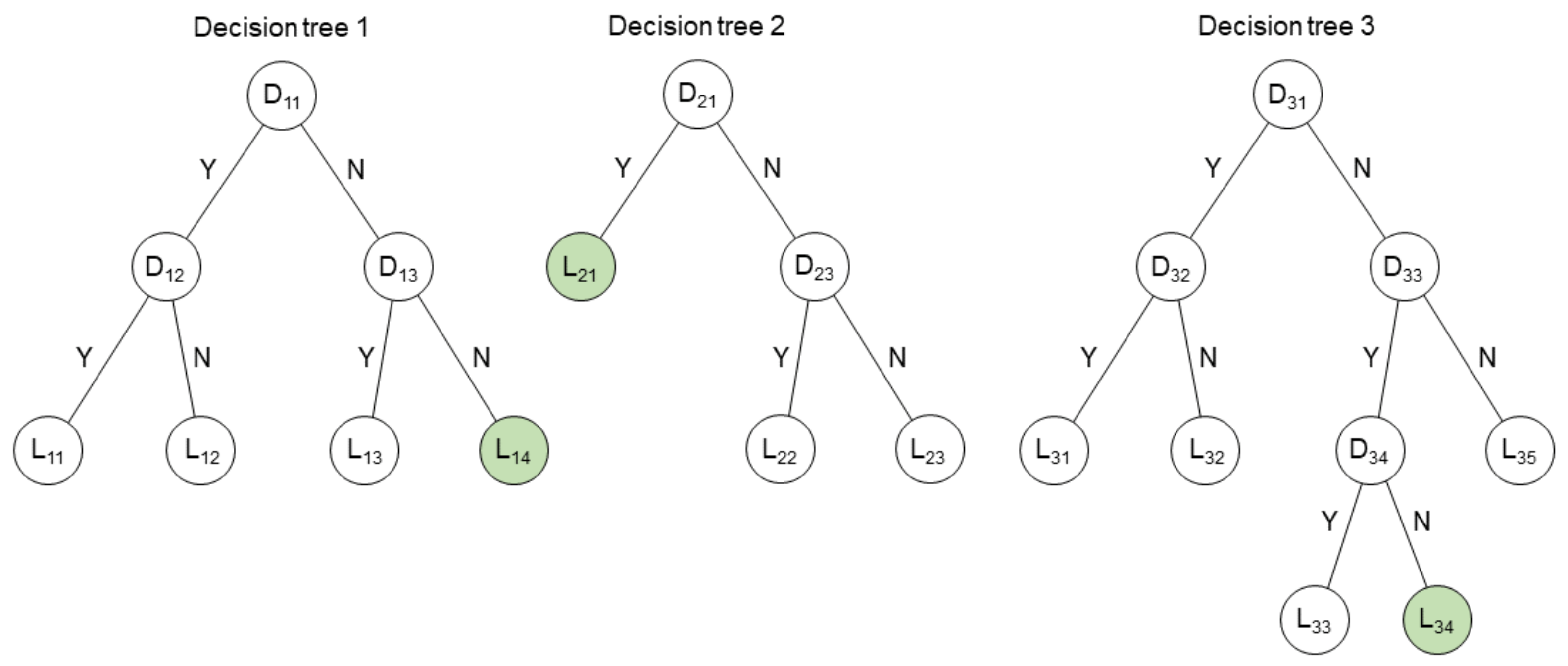
A decision tree is a graph consisting of decision and leaf nodes, examples of which are depicted in Figure 1. Every decision node () contains a split based on a condition pertaining to one of the features of the training data (e.g., is the angle of wave attack > ?). From a decision node, tree branches emerge for both possible answers. Each of these branches may be connected to either another decision node or a leaf node. A leaf node () is an end node that contains the prediction of either a class (classification trees) or a value (regression trees). A single decision tree consists of many splits on different features, where the number of subsequent splits is called the depth of the tree. Note that a single decision tree is often not sufficient to provide accurate predictions for highly complex classification or regression problems.
Instead of one single decision tree, GBDT methods use an ensemble of many decision trees that result in a communal prediction. An example of an ensemble of decision trees with a maximum depth of 3 is shown in Figure 1. The underlying principle is that combining large numbers of weak predictors can make for a strong predictor. Subsequent trees are iteratively added to the ensemble, trying to correct for prediction errors of previous trees. The final answer of the ensemble of trees is the sum of all predictions of the individual trees (the green leaf nodes in Figure 1), accounting for the learning rate (see Section 3.1). The total number of trees within the ensemble can either be set at the start of training, or use can be made of an ‘early stopping’ algorithm, which is explained in more depth in Section 3. In this paper, the GBDT implementation used is XGBoost [8] (XGB) as a package in Python [13].
2.2. Training Data Set
The CLASH database [4] contains the results of more than 10,000 data records of physical model experiments on wave overtopping. The resulting mean wave overtopping discharge, the test setup and the hydraulic loading conditions are represented by 31 parameters in the database.
Zanuttigh et al. [6] have collected additional wave overtopping data as an extension of the original database [4], and added data on wave transmission and reflection. Note that in this paper, a comparison is made with the NN by van Gent et al. [5], since the present research is focused on wave overtopping and the NN by Zanuttigh et al. [6] does not improve on the NN by van Gent et al. [5]. Hence, the same database [4] as applied by van Gent et al. [5] is used here. Neither of the NN models use all available parameters from the database. To get to a training data set, features (i.e., model input parameters) to train on are selected, unreliable or unsuitable data is removed, a weight factor is determined for each data record and scaling is applied. These selection, cleaning, and pre-processing steps are expanded upon below.
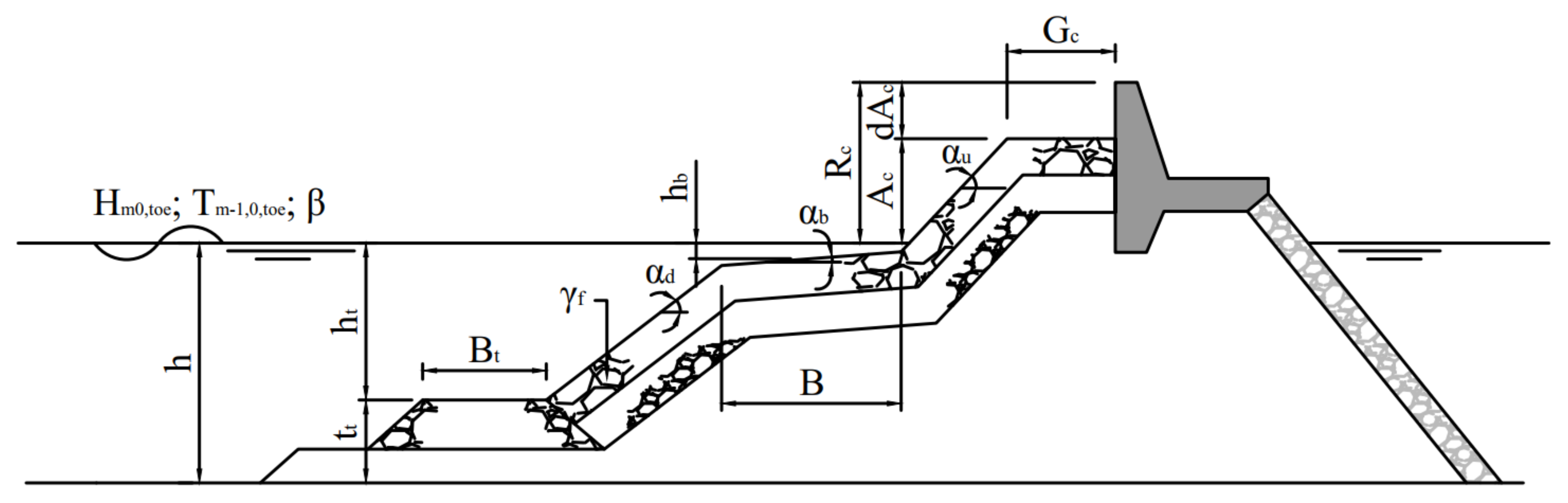
Only a selection of all available features in the database is used to train the model. The features used in the XGB and NN models are listed in Table 1 and illustrated in Figure 2, which also contains the features resulting from feature engineering, as discussed in Section 3.2. Note that the complexity () and reliability factors () are only used for weighting the different records in the training data set with a weight factor (). The weighting formula from van Gent et al. [5] is used: . This way, the most reliable and least complex data has the highest weight factor. This also means that the data records with either unreliable () or very complex data () are not included in the training data set. Besides the reliability factor and complexity factor scores for each data record, van Gent et al. [5] also argue that data records with a very small mean overtopping discharge (before Froude scaling) are less accurate due to potential scale effects, while the relevance for practical applications of these very small discharges (smaller than 0.001 l/s/m) is relatively low. Hence, in line with van Gent et al. [5], records with m/s/m are treated as , irrespective of their actual and scores. Additionally, the data records in the database that contain the remark ‘do not use for neural network’ have also been excluded from the training data set. In the end, the training database contains 8372 records.
Identical to van Gent et al. [5], all features in the training data set are scaled to m using Froude’s similarity law. Note that after scaling, the itself is not used as a feature in the model. In Table 1 the features to which Froude scaling applies are indicated in the last column. Additionally, the same target value is used, namely the of the Froude scaled mean wave overtopping discharge.
3. Model Training and Tuning
For the training of the XGB model and assessing its performance, functionalities from the scikit-learn package [14] in Python have been used. The model performance is optimized by tuning the model settings—its hyperparameters (Section 3.1)—and performing feature engineering (Section 3.2). The model is derived from a training data set, whose composition is discussed in Section 2.2. Note that, compared to the approach of van Gent et al. [5], some features of the training data set are adapted, following the outcome of the feature engineering.
3.1. Hyperparameter Tuning
The architecture and complexity of a single decision tree can be tuned by changing the depth of the tree and the number of leaf nodes allowed in a tree. Without any restrictions and with a sufficiently large ensemble of trees, GBDT methods are expected to overfit the training data set, in extreme cases creating very deep trees with in the limit a leaf node for every data point in the training data set. An overfitted model fits its training data very well, but does not have generic predictive capabilities on previously unseen data.
Within the XGB implementation, various hyperparameters to prevent overfitting are available and have been used in this work. Hyperparameters is an often used term in machine learning for the run control parameters of a method such as XGB. Firstly, the maximum depth of individual trees () has been limited to at most the amount of features used to train the model. The number of leaf nodes per tree are not directly limited, but every leaf node needs to contain a minimum number of data points in the training data set (). In this case, single data point leaves are prohibited to prevent overfitting. Additionally, the values of the leaf nodes are multiplied by a learning rate (), which also helps prevent overfitting. This is at the cost of a slower convergence, in that a larger number of trees are required in the ensemble. In machine learning, learning rate are commonly <0.1. A range of learning rate values adhering to this has been selected. High complexity of individual trees is undesirable, as it can be a source for overfitting. Tree complexity is therefore penalized with a regularization term which promotes smaller absolute values in the leaf nodes (). This regularization term is minimized in combination with the loss function (which represents the error w.r.t. the training data) in the training process. The selected values for ensure it is a relatively strictly enforced regularization. Finally, when adding a single new tree to the ensemble, only a portion of the records in the training data set is used to fit that tree (). This subsample is randomized for every added tree, thus counteracting overfitting on the level of individual trees. A range of values where subsample is active () is explored.
For the hyperparameter tuning of the XGB model, a grid search method is used, combined with K-fold cross-validation (using ). The hyperparameters considered for tuning and the combinations examined are listed in Table 2. All combinations of these hyperparameter values are used to train five different models, each with a different subsample (or fold) of the training data. Best hyperparameter values (indicated in blue) are selected based on the averaged best performance on the validation data set over all folds. The resulting optimal hyperparameter values favor deeper trees, in combination with fairly stringent overfitting prevention measures, consisting of significant regularization, a small learning rate, and a small data subsample to train each tree.
3.2. Feature Engineering and Feature Importance
A common practice in the improvement of the predictive capabilities of machine learning models is feature engineering. Features are those parameters selected from all available data to form the training data set. The term feature engineering describes the derivation of new parameters that provide either an addition to, or replacement of, existing features in the the training data set. The goal is to obtain new features that better describe the dependency (or sensitivity) of the target variable on the input parameters, improving the performance of machine learning models.
A useful tool to gain more insight into the different features in a machine learning model is feature importance analysis. For each individual feature, this provides an indication of its influence on the prediction of the target variable q. One way to perform this analysis is by looking at permutation importance [15,16]. In this work, the ELI5 [17] Python implementation of permutation importance has been used. This technique scrambles the values of one feature in the test data set. When scrambling all the data of an important feature, the predicted q should significantly change. Conversely, scrambling an unimportant feature will hardly affect the predicted q. The random scrambling of the data is repeated five times for each feature, and the whole process is applied to each feature individually, while keeping all other features unchanged.
Results of the permutation importance analysis before and after feature engineering performed below, are listed in Table 3. The results before feature engineering show that structure properties and are the most important features by far. Of the wave properties, the is the most important. Note that all features have been Froude scaled to a wave height of m, so the itself no longer shows up in the analysis. Surprisingly, the results also suggest that is a reasonably important feature, more important than for instance the berm width. This is misleading, however, and a direct result of the way some of the features are defined.
In the CLASH database features used in the NN, two features are strongly correlated to others: the armour crest freeboard () and the water depth above the toe structure (). The is defined as the distance between armour crest and still water level. When no armour is present, is taken to be equal to the crest freeboard (). Hence, the is by definition strongly correlated to . Similarly, the is equal to the water level at the toe (h) when no toe structure is present. This induces a strong correlation between the features and h.
The chosen way of defining these features makes it difficult to distinguish between the importance of correlated features. To gauge the actual importance of the armour crest freeboard and the toe dimensions for the prediction of q, the features need to be made uncorrelated. By replacing the armour crest freeboard with: , i.e., the distance between the crest and the armour crest freeboard (which is 0 when no armour layer is present), becomes uncorrelated to . Analogously, is replaced by the thickness of the toe structure: (which is 0 when no toe structure is present), where is uncorrelated to h. Both and are also illustrated in Figure 2.
On the right side of Table 3, the permutation importance after replacement of and with and respectively is shown. The changes larger then 10% are indicated by colours. The decrease of importance of and is shown in red, whereas the increase of importance in , h and is shown in green. Evidently, the correlated definitions of the features influence the perceived importance of the correlated features. The crest freeboard is now even more important, while the armour crest freeboard is less important for the prediction of the wave overtopping discharge. Interestingly, the importance of both the water level and the thickness of the toe structure has increased. Parallel to that, the importance of has decreased. Presumably, the water depth has gained in importance, where the importance of both the presence of a toe structure and its dimensions is now redistributed between the and features. Finally, the changes suggested not only remove correlation between different features, but also improve model quality resulting in a reduced error, see Table 4 and Section 4.
3.3. Bootstrap Resampling and Prediction Errors
In this work, the bootstrap resampling technique presented by van Gent et al. [5] is also applied to obtain estimates for the uncertainties in the model’s predictions. This approach is summarized as follows. From the total training data 500 bootstrap resamples are generated. Each bootstrap resample forms the training set for a new model and contains a different randomized selection from the total data set. In that training, the data points not selected in the resample serve as the validation data set. This validation set is used for ‘early stopping’, which stops the training of a single model after 1000 consecutive additional trees fail to improve the model performance on the validation data set. The data in the validation set also changes with each resample. In the end, this gives an ensemble of 500 retrained (’resampled’) models, where all suitable data is utilized while no single model is trained on the entire data set. All 500 models are run and the mean of all outcomes is used as the final prediction. Additionally, a confidence interval can also be determined from the large number of model predictions.
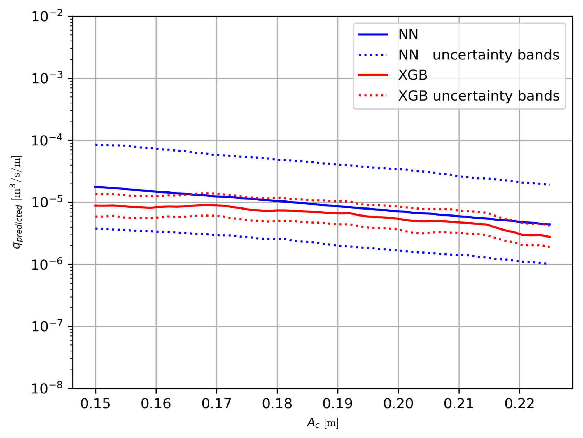
When applying the same technique with the XGB model, it is found that in this case the median of the 500 models is a better predictor than the mean (see Table 4). It seems that the tails of the distribution of the bootstrapped model predictions are not symmetrical, with the extremes tending to skew towards higher overtopping discharges. This is reflected in the mean, while is does not significantly affect the median. Thus, going forward, the median is used as prediction. Another surprising observation is that the confidence interval derived with the bootstrap resampling method becomes very small for the XGB model compared to the NN model, as can be seen in the example in Figure 3. This decrease is so significant that it cannot be satisfactorily explained as of yet. In fact, the way resampling must be used for GBDT-based models must be reconsidered since in the present approach the model architecture is not completely fixed due to randomness-inducing hyperparameters and can be different for each resample. For the moment, this is an issue for further investigation. Hence, in the rest of this work, the confidence interval based on bootstrap resampling is not used.
4. Model Validation
To validate the trained XGB model, its performance is compared to that of the NN by van Gent et al. [5], which can be accessed through the NN-Overtopping web application [18]. The NN is of the type Multi-Layer Perceptron, and contains a single hidden layer with 20 nodes, and is trained on the same training data set as the XGB model. The performance for both methods is quantified by predicting the records of the original CLASH database [4] and subsequently determining the root-mean-square-error (RMSE) identical to the method by van Gent et al. [5]. The RMSE is determined for the target variable, namely the of the Froude scaled mean wave overtopping discharge. These errors are weighted using the also used in the model training, as described in Section 2.2.
The resulting errors for the different models are shown in Table 4. It can be seen that the XGB model yields a large improvement of the existing NN, reducing the RMSE with a factor of 2.8. The switch in machine learning method from NN to XGB is responsible for the majority of the reduction in error (from 0.29 to 0.168). Additional error reduction is accomplished by the redefinition of features detailed in Section 3.2 and using the median instead of the mean as prediction.
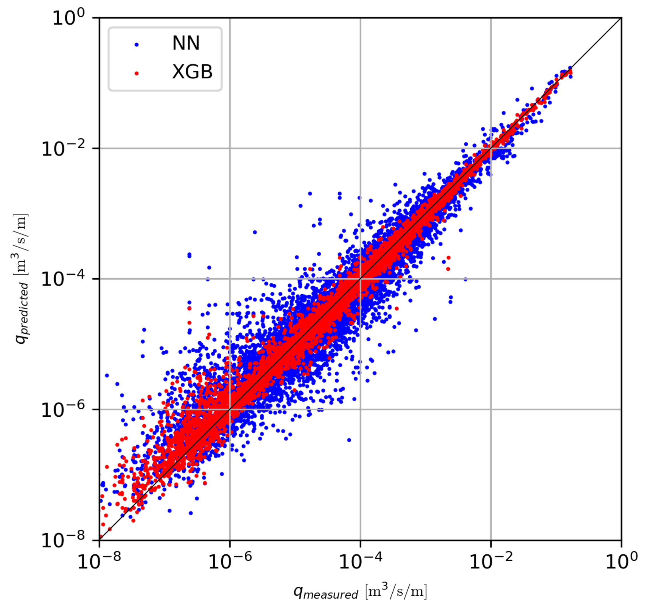
The measurements from the database and the predictions thereof by the NN and the XGB model (median) are mutually compared through scatter plots, see Figure 4. The smaller RMSE for the XGB model can be recognized from the smaller spread in the red points around the diagonal (i.e., better predictions) than the spread in the blue points. The red points belonging to m/s/m show noticeably larger deviations from the measurements, which is a reflection of the lowering of the for those points, as described in Section 2.2.
5. Model Verification
After training the XGB model, the behaviour of the model is qualitatively verified using synthetic data sets. First, the model is checked for physically realistic behaviour, i.e., a reasonably smooth behaviour that confirms the expectations following from the understanding of the physics behind wave overtopping. This is done by varying one feature at a time (Section 5.1). Subsequently, the behaviour of the model in the data sparse regions of the input parameter space is visualized, by detailed examination of the space in between clusters of training data points (Section 5.2).
5.1. Physical Realism for Single Feature Variations
To assess the physical realism displayed by the XGB model, the results along one line segment varying a single feature are plotted versus the log of the wave overtopping discharge. To this end, 1288 data points for realistic reference situations have been synthesized, two examples of which are further discussed and shown in Figure 5 with feature values listed in Table 5. For comparison, the results from the NN are also plotted. Note that both lines show model behaviour, but neither represents an objective truth.
From Figure 2 it is evident that for an increasing crest freeboard (), the overtopping discharge is expected to decrease. Figure 5a shows that this indeed is the general trend. The XGB model, however, shows non-smooth behaviour that locally causes increases in discharge with increasing freeboard. Figure 5b shows that, as expected, the wave overtopping discharge decreases with an increasingly oblique angle of wave attack. However, where the NN is reasonably smooth, the XGB model does not predict a smooth decrease of the wave overtopping discharge, but rather shows a staircase pattern. Both the staircase pattern for wave obliquity and the non-smooth behaviour for the freeboard are inherent traits of GBDT methods. Since the method is based on an ensemble of CARTs, it features many discrete splits in regression trees. This leads to the discontinuous behaviour seen in Figure 5. The size and density of the discontinuities in the model’s predictions depend in large amount on both the number of trees and number of data points along the axis of interest. For instance, there are relatively few data points with a (11.5% of the training data), so given that q decreases with increasing , this will inevitably result in the discrete staircase behaviour observed in Figure 5b. An abundance of data points along the axis of interest allows GBDT methods to distinguish with higher resolution between different values of a certain feature. Hence, it is a requirement, but not a guarantee for smooth behaviour. Methods that allow for locally optimized fits—such as GBDT—can result in variations around a general trend. This is exhibited in Figure 5a. Note that, while non-smooth model behaviour is in principle not desirable, it might be a worthwhile tradeoff if the model predictions are more accurate on the whole.
5.2. Regularity of Predictions Throughout the Input Space
Because of their data-driven nature, GBDT models are expected to exhibit relatively good performance in regions of the input parameter space with a high density of training patterns, since there is ample information present to fit the model to. This is contrasted by the data sparse regions of the input parameter space, where relatively very few points from the training data set are available. The question is whether the model performance in those regions is not completely erratic. To answer this question, a data cluster analysis is performed to locate the regions in the input space with the largest density of data points. Subsequently, XGB and NN model predictions are made (13,132 in total) for the line segments connecting the cluster centres. In this way, large parts of the input space are covered, including low data density regions.
In a data cluster analysis, a meaningful distance metric must be provided. Since the features of the training data set have various different units and absolute magnitudes, these features need to be normalized to be able to measure distances in a meaningful way. To this end, firstly all features are z-scaled using , where x is the feature in question, is the mean of feature x and is its standard deviation. Subsequently, a Principle Component Analysis (PCA) is carried out to determine the principal directions of the data. Finally, the data is redefined using this PCA coordinate system, resulting in a measure of distance that takes the data coverage per principal direction into account. In this new coordinate system, K-means clustering is used to find clusters of data points that are close to each other. Outside of these clusters are the data sparse regions of the input parameter space. Given this sparsity, it is interesting to see how data-driven models behave in these regions.
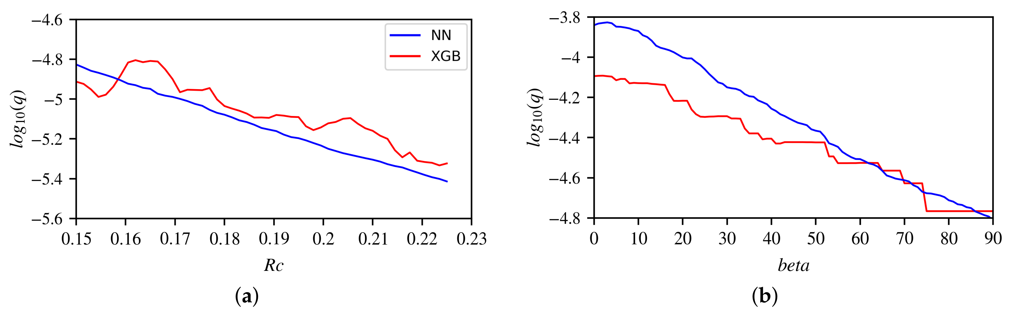
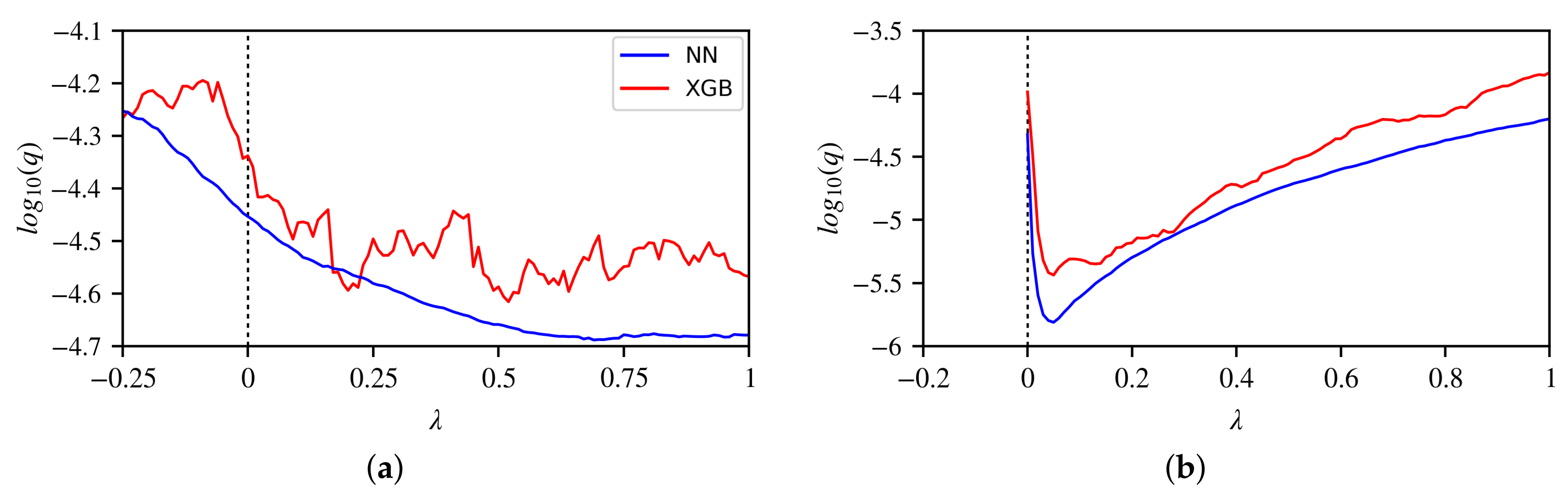
In Figure 6 the behaviour of the predictions of the XGB model is shown for two examples: the two cluster centres closest and most distant from each other. The is a coordinate for the straight line that connects one cluster centre to another. The coordinate is defined as 0 in one cluster centre and 1 in the other. As a reference, the behaviour of the NN is also depicted. Note that on the path between the two cluster centres, in contract to the analysis in Section 5.1, all of the features are changing simultaneously. Thus, no expected response can be realistically formulated, and only an inter-model comparison remains. Figure 6a shows the model response between two cluster centres that are close to each other. The XGB model behaves less smoothly than the NN, comparable to what was found in Section 5.1. The general trend does seem somewhat similar between both models, especially given the limited range on the vertical axis. In contrast, Figure 6b depicts two cluster centres that are distant from each other. In spite of the large distance, the behaviour of both models is quite similar.
The model response between both the close and distant cluster centres shows that there is no uncontrolled or erratic model behaviour in the data sparse regions of the input parameter space. The XGB model can show some non-smooth behaviour but the large-scale general trends are reasonably similar to those displayed by the NN model.
Note that, while the model verification using synthetic data described above gives insight in model behaviour, it does not show whether or not the model is overfitted. Though efforts are made to prevent overfitting (as described in Section 3), they provide no guarantee. Furthermore, the validation method used, consistent with existing literature [5], does not necessarily preclude overfitting. A definitive answer to the question of whether or not the model is overfitted should be obtained by validating the model against new physical model data that are not part of the model training. Good performance on this unseen data suggests generic applicability of the model, while bad performance is an indication of an overfitted model.
6. Discussion
The training data set for the new predictive model presented in this work is based on a selection of data from the CLASH database, similar to earlier efforts in literature [5,6]. Not all data records from the database—neither the original, nor the extended version—are equally reliable or usable to train data driven models (see also the considerations in Section 2.2). In addition to the reliability factor and complexity factor of the data, various other causes may reduce the reliability and thus the usability of particular data records. Firstly, the database records with small measured q are likely to be less reliable, given the large relative measurement uncertainty in those situations. Furthermore, some features in the database records originate from inference or numerical model computations rather than direct measurements. This introduces additional uncertainties which are currently not taken into account. Besides data quality, quantity of available training data is also an important factor in the use of data-driven methods. This is underlined by the data cluster analysis, which shows model behaviour deviates mostly in regions with low data density. Hence, the training data set should ideally be continuously expanded with new data points, especially those lying within data sparse regions.
The model verification against synthetic data sets shows that the new XGB model in general behaves reasonably well, but does show non-smooth behaviour in some situations. This essentially comes down to small scale oscillations around a larger trend. In the cases investigated in this work, the trend was similar to the one shown by the NN model. The non-smooth behaviour is inherent to the discontinuous nature of methods that use decision trees, and thus not entirely avoidable. The observed non-smooth behaviour is in principle undesirable. However, the large scale trends are captured well by the XGB model and its predictions are a significant improvement. Hence, we find the non-smooth behaviour to be a worthwhile tradeoff.
The application of bootstrap resampling results in accurate predictions but a surprisingly small prediction error, as described in Section 3.3. One of the contributing factors to this might be the effect of the hyperparameters preventing overfitting (such as , and ). These hyperparameters create a more generalized model, less dependent on the specific data points included in the data set. This means that the different bootstrap resamples will result in more similar models and thus smaller prediction errors that do not fully explain the variation in the underlying training data. Investigation of a conceptual approach to estimate uncertainties for GBDT-based models is a subject of further research.
In this work and existing research, the performance of machine learning methods is quantified based on the prediction of different iterations of the CLASH database. However, (parts of) those databases are also used for model training. An important following step is to test the model performance on new physical model data as of yet unseen by the model. If the XGB model also predicts this data accurately, relative to the alternative overtopping prediction methods, the confidence in the generic applicability for engineering and design purposes is further solidified. This is especially true for new data that covers the currently data sparse regions of the input parameter space.
7. Conclusions and Recommendations
In this paper, an innovative machine learning technique called gradient boosting decision trees has been applied to the prediction of mean wave overtopping discharges. The training and tuning of the model have been extensively described. A feature engineering analysis shows that redefining existing features in the CLASH database (without adding new information) can improve the model’s performance. The new XGBoost model has been shown to outperform the existing neural network model [5] by reducing the error on the prediction of the CLASH database by a factor of 2.8. Additionally, the new model shows physically realistic trends along important features, and seems to behave coherently in the data sparse regions of the input space.
The prediction errors of the XGB model determined by bootstrap resampling are considered to by surprisingly small, seemingly not fully explaining the variation in underlying the training data. For future research, it is recommended to investigate in more detail a proper conceptual approach for the estimation of uncertainties in the predictions of GBDT-based models.
The promising results presented in this work suggest an application of Gradient Boosting to an extended database as a logical next step. Furthermore, comparison should be made to other available prediction methods for the wave overtopping discharge, including empirical wave overtopping formulae.
The confidence in the predictive capabilities and generic applicability of the model in engineering and design purposes further increases when it also performs well on unseen data. In addition, good performance on unseen data suggests that the model is not overfitted. Hence, it is strongly recommended to perform further model validation on new data as of yet unseen by the model.
Author Contributions
Conceptualization, J.P.d.B.; methodology, J.P.d.B., J.M.W., H.F.P.v.d.B. and M.R.A.v.G.; software, J.P.d.B., J.M.W. and H.F.P.v.d.B.; validation, H.F.P.v.d.B., J.P.d.B. and J.M.W.; formal analysis, J.P.d.B.; writing—original draft preparation, J.P.d.B.; writing—review and editing, J.P.d.B., J.M.W., H.F.P.v.d.B. and M.R.A.v.G.; visualization, H.F.P.v.d.B. and J.P.d.B.; supervision, M.R.A.v.G.; project administration, M.R.A.v.G. All authors have read and agreed to the published version of the manuscript.
Funding
This research was funded in part by the Deltares Strategic Research programme “Future-proof coastal infrastructure & offshore renewable energy”.
Acknowledgments
The authors wish to thank Alex Capel and Paul van Steeg for the insightful discussions on wave overtopping.
Conflicts of Interest
The authors declare no conflict of interest.
References
- TAW. Wave Run-Up and Wave Overtopping at Dikes; Technical Report; Technical Advisory Committee for Flood Defence in the Netherlands (TAW): Delft, The Netherlands, 2002. [Google Scholar]
- EurOtop. Wave Overtopping of Sea Defences and Related Structures: Assessment Manual. Pullen, T., Allsop, N.W.H., Bruce, T., Kortenhaus, A., Schüttrumpf, H., van der Meer, J.W., Eds.; 2007. Available online: https://www.google.com/url?sa=t&rct=j&q=&esrc=s&source=web&cd=&cad=rja&uact=8&ved=2ahUKEwjNvvyrioPqAhVPCqYKHTOvBSoQFjABegQIAxAB&url=http%3A%2F%2Fwww.kennisbank-waterbouw.nl%2FDesignCodes%2FEurOtop.pdf&usg=AOvVaw3ZxFfURm8QaIJ2JzOR0PXl (accessed on 27 November 2019).
- EurOtop. Manual on Wave Overtopping of Sea Defences and Related Structures. An Overtopping Manual Largely Based on European Research, but for Worldwide Application. van der Meer, J.W., Allsop, N.W.H., Bruce, T., de Rouck, J., Kortenhaus, A., Pullen, T., Schüttrumpf, H., Troch, P., Zanuttigh, B., Eds.; 2018. Available online: www.overtopping-manual.com (accessed on 27 November 2019).
- Steendam, G.J.; Van der Meer, J.W.; Verhaeghe, H.; Besley, P.; Franco, L.; Van Gent, M.R.A. The international database on wave overtopping. Coast. Eng. 2005, 4301–4313. [Google Scholar] [CrossRef] [Green Version]
- Van Gent, M.R.A.; Van den Boogaard, H.F.P.; Pozueta, B.; Medina, J.R. Neural network modelling of wave overtopping at coastal structures. Coast. Eng. 2007, 54, 586–593. [Google Scholar] [CrossRef] [Green Version]
- Zanuttigh, B.; Formentin, S.M.; Van der Meer, J.W. Prediction of extreme and tolerable wave overtopping discharges through an advanced neural network. Ocean. Eng. 2016, 127, 7–22. [Google Scholar] [CrossRef]
- Jensen, B.; Jacobsen, N.G.; Christensen, E.D. Investigations on the porous media equations and resistance coefficients for coastal structures. Coast. Eng. 2014, 84, 56–72. [Google Scholar] [CrossRef]
- Chen, T.; Guestrin, C. XGBoost: A Scalable Tree Boosting System. arXiv, 2016; arXiv:1603.02754. [Google Scholar]
- Ke, G.; Meng, Q.; Finley, T.; Wang, T.; Chen, W.; Ma, W.; Ye, Q.; Liu, T.Y. LightGBM: A Highly Efficient Gradient Boosting Decision Tree. In Advances in Neural Information Processing Systems 30; Guyon, I., Luxburg, U.V., Bengio, S., Wallach, H., Fergus, R., Vishwanathan, S., Garnett, R., Eds.; Curran Associates Inc.: Nice, France, 2017; pp. 3146–3154. [Google Scholar]
- Kaggle Team. Your Year on Kaggle: Most Memorable Community Stats from 2016. 2017. Available online: http://blog.kaggle.com/2017/01/05/your-year-on-kaggle-most-memorable-community-stats-from-2016/ (accessed on 3 December 2019).
- Kazeminezhad, M.H.; Etemad-Shahidi, A. A new method for the prediction of wave runup on vertical piles. Coast. Eng. 2015, 98, 55–64. [Google Scholar] [CrossRef]
- Ellenson, A.; Pei, Y.; Wilson, G.; Özkan Haller, H.T.; Fern, X. An application of a machine learning algorithm to determine and describe error patterns within wave model output. Coast. Eng. 2020, 157, 103595. [Google Scholar] [CrossRef]
- Van Rossum, G. Python Tutorial; Technical Report CS-R9526; Centrum voor Wiskunde en Informatica (CWI): Amsterdam, The Netherlands, 1995. [Google Scholar]
- Pedregosa, F.; Varoquaux, G.; Gramfort, A.; Michel, V.; Thirion, B.; Grisel, O.; Blondel, M.; Prettenhofer, P.; Weiss, R.; Dubourg, V.; et al. Scikit-learn: Machine Learning in Python. J. Mach. Learn. Res. 2011, 12, 2825–2830. [Google Scholar]
- Breiman, L. Random forests. Mach. Learn. 2001, 45, 5–32. [Google Scholar] [CrossRef] [Green Version]
- Fisher, A.; Rudin, C.; Dominici, F. All Models are Wrong, but Many are Useful: Learning a Variable’s Importance by Studying an Entire Class of Prediction Models Simultaneously. arXiv, 2018; arXiv:stat.ME/1801.01489. [Google Scholar]
- ELI5 Python Package. Available online: https://github.com/TeamHG-Memex/eli5 (accessed on 31 March 2020).
- Deltares. Overtopping Neural Network Webtool. Available online: https://www.deltares.nl/en/software/overtopping-neural-network/ (accessed on 8 April 2020).
Figure 1.
Schematic depiction of an ensemble of decision trees with decision () and leaf nodes (). An example prediction for one combination of input parameters is shown in green.
Figure 1.
Schematic depiction of an ensemble of decision trees with decision () and leaf nodes (). An example prediction for one combination of input parameters is shown in green.

Figure 2.
Feature definitions, adapted from van Gent et al. [5].
Figure 2.
Feature definitions, adapted from van Gent et al. [5].

Figure 3.
Wave overtopping predictions from the NN [5] (blue) and XGB (orange) models versus armour crest freeboard, including confidence interval from bootstrap resampling (dotted lines).
Figure 3.
Wave overtopping predictions from the NN [5] (blue) and XGB (orange) models versus armour crest freeboard, including confidence interval from bootstrap resampling (dotted lines).

Figure 4.
Predicted versus measured wave overtopping discharge for the CLASH database. Predictions from the NN by van Gent et al. [5] (blue) and new XGB model (red).
Figure 4.
Predicted versus measured wave overtopping discharge for the CLASH database. Predictions from the NN by van Gent et al. [5] (blue) and new XGB model (red).

Figure 5.
Predictions from the NN (blue) and XGB (red) for variation in crest freeboard (a) and angle of wave attack (b).
Figure 5.
Predictions from the NN (blue) and XGB (red) for variation in crest freeboard (a) and angle of wave attack (b).

Figure 6.
Predictions from the NN (blue) and XGB (red) models between cluster centres, where is the coordinate on a straight line from one cluster centre to another. (a) Two cluster centres closest to each other. (b) Two most distant cluster centres.
Figure 6.
Predictions from the NN (blue) and XGB (red) models between cluster centres, where is the coordinate on a straight line from one cluster centre to another. (a) Two cluster centres closest to each other. (b) Two most distant cluster centres.


Table 1.
Overview of target variable and the features used in model training in the NN by van Gent et al. [5] and the new XGB model. Froude scaling of features is indicated in the last column.
Table 1.
Overview of target variable and the features used in model training in the NN by van Gent et al. [5] and the new XGB model. Froude scaling of features is indicated in the last column.
| Name | Symbol | Unit | NN | XGB | Fr Scaled |
|---|---|---|---|---|---|
| Mean wave overtopping discharge | q | m/s/m | ✓ | ✓ | ✓ |
| Water depth, toe | h | m | ✓ | ✓ | ✓ |
| Spectral significant wave height, toe | m | ✓ | ✓ | - | |
| Spectral wave period, toe | s | ✓ | ✓ | ✓ | |
| Angle of wave attack | ✓ | ✓ | - | ||
| Roughness factor of the structure | - | ✓ | ✓ | - | |
| Cotangent of the lower slope | - | ✓ | ✓ | - | |
| Cotangent of the upper slope | - | ✓ | ✓ | - | |
| Crest freeboard | m | ✓ | ✓ | ✓ | |
| Armour crest freeboard | m | ✓ | - | ✓ | |
| Difference between crest and armour crest freeboard | m | - | ✓ | ✓ | |
| Crest width | m | ✓ | ✓ | ✓ | |
| Width of the berm | B | m | ✓ | ✓ | ✓ |
| Water depth above the berm | m | ✓ | ✓ | ✓ | |
| Tangent of berm slope | - | ✓ | ✓ | - | |
| Water depth above the toe structure | m | ✓ | - | ✓ | |
| Thickness of the toe structure | m | - | ✓ | ✓ | |
| Width of the toe structure | m | ✓ | ✓ | ✓ | |
| Complexity factor | - | ✓ | ✓ | - | |
| Reliability factor | - | ✓ | ✓ | - |
Table 2.
XGB hyperparameter combinations used in the K-fold cross-validation, optimal values in blue.
Table 2.
XGB hyperparameter combinations used in the K-fold cross-validation, optimal values in blue.
| Hyperparameter | Name | Values |
|---|---|---|
| Maximum tree depth | 6; 7; 8; 10; 12; 14 | |
| Minimum number of data points in a leaf | 3; 5; 7; 10; 12 | |
| Learning rate | 0.005; 0.0075; 0.01; 0.02; 0.05 | |
| L2 regularization parameter | 2; 3; 4 | |
| Subsampled fraction of training data | 0.25; 0.50; 0.75 |
Table 3.
Overview of permutation importance results before and after feature engineering. Weight changes >10% indicated in green (increase) and red (decrease). Changes in rank are indicated with arrows and green (increase) or red (decrease) numbers.
Table 3.
Overview of permutation importance results before and after feature engineering. Weight changes >10% indicated in green (increase) and red (decrease). Changes in rank are indicated with arrows and green (increase) or red (decrease) numbers.
| Before | After | ||||
|---|---|---|---|---|---|
| Rank | Feature | Weight | Feature | Weight | |
| 1 | 0.6666 ± 0.0204 | - | 0.8939 ± 0.0369 | ||
| 2 | 0.5992 ± 0.0437 | - | 0.6063 ± 0.0456 | ||
| 3 | 0.1979 ± 0.0194 | - | 0.2000 ± 0.0199 | ||
| 4 | 0.1354 ± 0.0085 | - | 0.1318 ± 0.0093 | ||
| 5 | 0.0935 ± 0.0097 | - | 0.0915 ± 0.0092 | ||
| 6 | 0.0765 ± 0.0034 | 4 ↑ | h | 0.0628 ± 0.0029 | |
| 7 | 0.0604 ± 0.0042 | - | 0.0614 ± 0.0040 | ||
| 8 | B | 0.0575 ± 0.0044 | - | B | 0.0608 ± 0.0045 |
| 9 | 0.0544 ± 0.0038 | - | 0.0544 ± 0.0040 | ||
| 10 | h | 0.0453 ± 0.0019 | 2 ↑ | * | 0.0363 ± 0.0040 |
| 11 | 0.0389 ± 0.0043 | 5 ↓ | * | 0.0340 ± 0.0046 | |
| 12 | 0.0312 ± 0.0040 | 1 ↓ | 0.0237 ± 0.0029 | ||
| 13 | 0.0085 ± 0.0014 | - | 0.0091 ± 0.0010 | ||
| 14 | 0.0016 ± 0.0003 | - | 0.0016 ± 0.0003 |
* and are replaced by the uncorrelated features and respectively.
Table 4.
Performance of different overtopping prediction tools.
| Tool | RMSE |
|---|---|
| NN Overtopping van Gent et al. [5] (mean) | 0.29 |
| XGB without feature engineering (mean) | 0.168 |
| XGB without feature engineering (median) | 0.130 |
| XGB with feature engineering (mean) | 0.149 |
| XGB with feature engineering (median) | 0.104 |
Table 5.
Feature values in physical realism analysis.
| Feature | Case | Case |
|---|---|---|
| h | 0.225 m | 0.225 m |
| 0.15 m | 0.15 m | |
| 2.00 s | 2.00 s | |
| 0 | 0–90 | |
| 0.5 | 0.5 | |
| 4 | 4 | |
| 2.5 | 2.5 | |
| 0.15–0.225 m | 0.15 m | |
| 0.00–0.075 m | 0.05 m | |
| 0.225 m | 0.225 m | |
| B | 0.45 m | 0.075 m |
| 0 m | 0 m | |
| 0 | 0 | |
| 0 m | 0 m | |
| 0 m | 0 m | |
| 1.5 | 1.5 | |
| 1–1.5 | 1 | |
| 0–0.5 | 0.33 | |
| 3 | 0.5 |
© 2020 by the authors. Licensee MDPI, Basel, Switzerland. This article is an open access article distributed under the terms and conditions of the Creative Commons Attribution (CC BY) license (http://creativecommons.org/licenses/by/4.0/).
Share and Cite
MDPI and ACS Style
den Bieman, J.P.; Wilms, J.M.; van den Boogaard, H.F.P.; van Gent, M.R.A. Prediction of Mean Wave Overtopping Discharge Using Gradient Boosting Decision Trees. Water 2020, 12, 1703. https://0-doi-org.brum.beds.ac.uk/10.3390/w12061703
AMA Style
den Bieman JP, Wilms JM, van den Boogaard HFP, van Gent MRA. Prediction of Mean Wave Overtopping Discharge Using Gradient Boosting Decision Trees. Water. 2020; 12(6):1703. https://0-doi-org.brum.beds.ac.uk/10.3390/w12061703
Chicago/Turabian Styleden Bieman, Joost P., Josefine M. Wilms, Henk F. P. van den Boogaard, and Marcel R. A. van Gent. 2020. "Prediction of Mean Wave Overtopping Discharge Using Gradient Boosting Decision Trees" Water 12, no. 6: 1703. https://0-doi-org.brum.beds.ac.uk/10.3390/w12061703
Note that from the first issue of 2016, this journal uses article numbers instead of page numbers. See further details here.