Comparison of Baseflow Separation Methods in the German Low Mountain Range


Chair of Engineering Hydrology and Water Management, Technical University of Darmstadt, 64287 Darmstadt, Germany
*
Author to whom correspondence should be addressed.
Water 2020, 12(6), 1740; https://0-doi-org.brum.beds.ac.uk/10.3390/w12061740
Submission received: 27 May 2020
/
Revised: 15 June 2020
/
Accepted: 16 June 2020
/
Published: 18 June 2020
(This article belongs to the Section Hydrology)
Abstract
:The last several years in southern Germany brought below average precipitation and high temperatures, leading to considerable challenges in water resource management. Deriving a plausible baseflow estimate is important as it affects aspects of integrated water resource management such as water usage and low flow predictions. The aim of this study is to estimate baseflow in a representative catchment in the German low mountain range and identify suitable baseflow estimation methods for this region. Several different baseflow separation methods, including digital filters, a mass balance filter (MBF) and non-continuous estimation methods were applied and compared to estimate baseflow. Using electric conductivity (EC) for the MBF, June to September and November to May were found to be suitable to estimate the EC of the baseflow and runoff component, respectively. Both weekly and continuous EC monitoring can derive similar EC value component estimates. However, EC estimation of the runoff component requires more careful consideration. The baseflow index (BFI) is estimated to be in the range of 0.4 to 0.5. The Chapman and Maxwell filter, Kille method and the Q90/Q50 ratio are recommended for baseflow estimation in the German low mountain range as they give similar results to the MBF. The Eckhardt filter requires further calibration before application.
1. Introduction
In recent years southern Germany has experienced several dry years with below average precipitation and high temperatures resulting in extended and/or severe low flow periods. Since 2003 there have hardly been any unusually wet years in southern Germany [1]. This has led to considerable challenges in water management [2]. In this context assessing baseflow in a catchment is of increased importance as the baseflow may impact many different aspects of integrated water resource management, e.g., water usage, water quality and low flow predictions. However, baseflow is not readily measurable and must be quantified indirectly. Many different methods exist to separate baseflow from the total observed flow. For instance, these methods encompass graphical methods, recession analysis, recursive digital filtering methods, as well as isotope or other stream constituents-based separation methods [3,4,5]. Graphical methods separate baseflow by identifying specific points in the hydrograph and connecting them via some predefined rule to account for the shape of the curve between these points [6,7,8]. These methods are however often not suited for automation and are susceptible to subjective influences [9,10]. Recession analysis assumes that periods without precipitation and with receding flow can be analyzed to infer knowledge on aquifer properties [11]. Commonly a master recession curve (MRC) is constructed to represent a catchment’s typical recession behavior [7,12]. Aquifer characteristics are either derived from the MRC or from individual recession periods. One commonly identified characteristic is the recession coefficient k, which is representative of the discharge-storage relationship of a linear reservoir [13,14]. However, research has shown that the assumption of linearity may not be valid in many catchments [15,16]. Therefore, nonlinear reservoir models are also commonly used to model recession periods and separate baseflow from total flow [14,17,18]. Recursive digital filters (RDFs) apply concepts from signal analysis to separate baseflow from total flow [19,20,21,22]. The number of filter parameters typically varies between one to three parameters, which need to be estimated prior to applying the filter to observed flow data [10]. RDFs are easily automated, and results can be reproduced; however, with their background being signal analysis their parameters may lack hydrological meaning [10]. Combinations of different methods have been reported in the literature as well [23,24]. Aksoy et al. [23] developed a combined method called the filtered smooth minima separation method in which baseflow is first separated by identifying baseflow turning points in the hydrograph and then applying an RDF to the separated baseflow hydrograph. All mentioned methods typically only require daily flow observation making them easily usable in many catchments. However, methods using precipitation data as well as flow data, e.g., [10,24], exist, and analysis has been conducted at event time scale, e.g., hourly resolution [24]. Tracer-based separation methods require more data but have been used for many years as well [3,25,26,27]. In addition to flow data, either data on one or more stable isotopes and/or geochemical tracers are required. Tracer-based baseflow separation using stable isotopes is labor and cost intensive. Therefore, geochemical tracers such as electric conductivity (EC) are often used [27]. It is assumed that each flow component has a distinct signature, and therefore, by applying mass balance techniques the flow components can be separated [26,27]. It is apparent that due to the manifold available baseflow separation methods it is necessary to apply several of these in order to identify a plausible baseflow estimate. This holds especially true when studying a new research basin, such as the Fischbach catchment in the federal state of Hesse, Germany, near the city of Darmstadt. The Fischbach is a tributary of the river Gersprenz and the entire Gersprenz catchment is the experimental field laboratory of the Chair of Engineering Hydrology and Water Management (ihwb) of the Technical University of Darmstadt. The Fischbach catchment was selected as a sub-catchment for detailed hydrological process research [28].
The objectives of this study are:
- Compile and analyze already existing long-term and newly measured high-resolution data to determine a plausible baseflow estimate for the new research basin;
- Examine the use of EC for mass balance filtering in the German low mountain range;
- Compare different types of baseflow separation methods and identify suitable methods for the German low mountain range.
Recession analysis and three methods of constructing an MRC are used in combination with three filter algorithms to give continuous baseflow estimates. Furthermore, a mass balance filter method (MBF) based on measurements of EC is applied as well. Special consideration is given to the determination of the MBF’s parameters and the required length of the measurement campaigns for reliable estimates. The results from two further methods, which only allow for a mean baseflow estimate, are also included in the comparison of the determined baseflow estimates.
2. Materials and Methods
2.1. Study Site
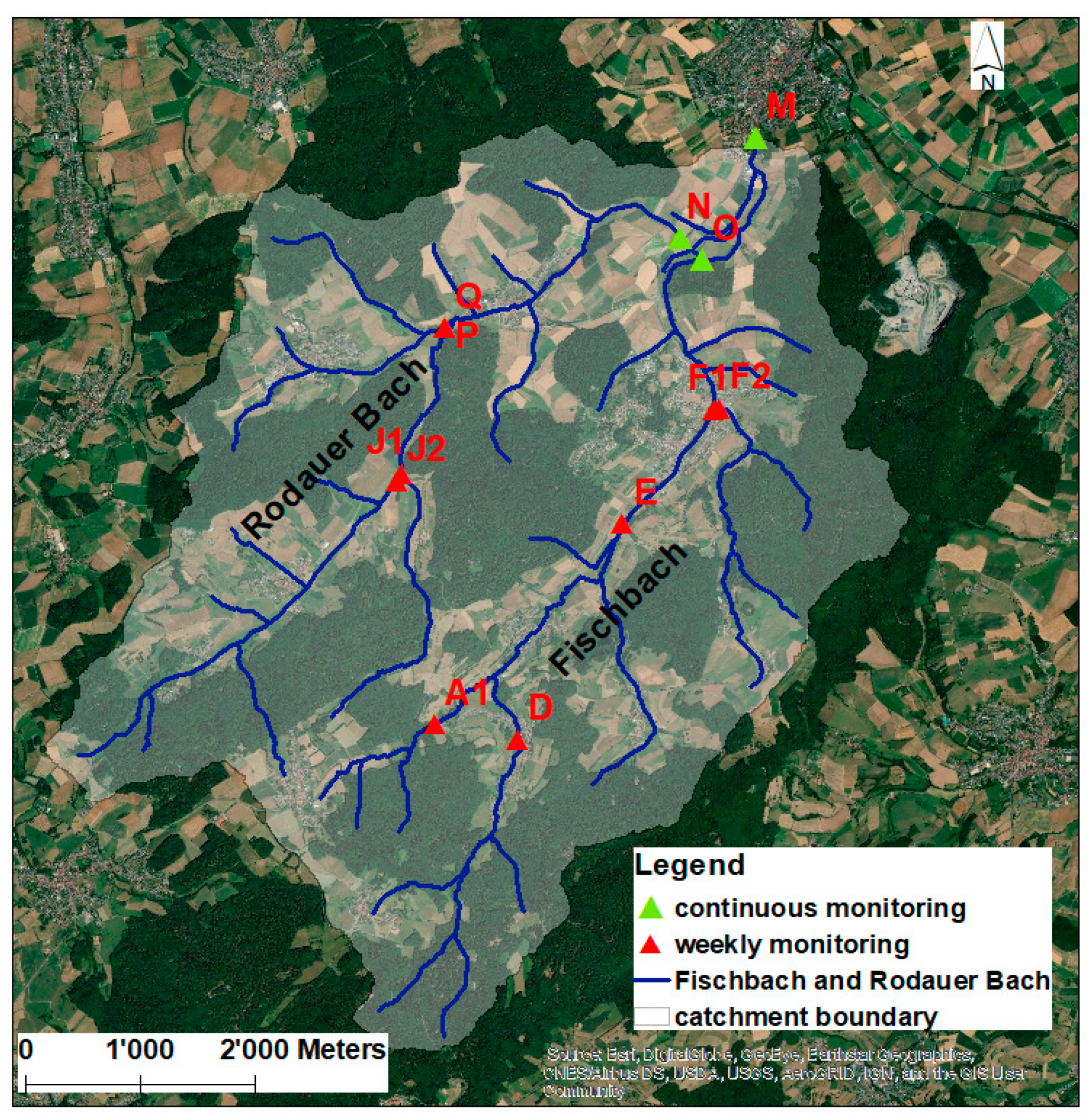
The Fischbach catchment, see Figure 1, is in the German low mountain range in the federal state of Hesse, Germany. It lies to the southeast of the city of Darmstadt and is part of the research catchment of the river Gersprenz, which is operated by the Chair of Engineering Hydrology and Water Management (ihwb) of the Technical University of Darmstadt. The Gersprenz catchment covers an area of approximately 485 km2. The Fischbach is a tributary to the Gersprenz. Its catchment, defined by a flow gaging station, has an area of 35.6 km2. At its highest point it has an elevation of nearly 600 m a.s.l. and at its lowest point of about 160 m a.s.l. The land use within the catchment is mostly rural and is characterized by forests and vegetation (51.7%) as well as arable land and grasslands (41.8%). Settlements account for 6.5% of the area [28]. Soils are mainly cambisols and alisols—the latter formed from quaternary loess layers and the former from grus over the crystalline basement complex.
The Fischbach is the main stream channel within the catchment and has one major tributary, the Rodauer Bach, which flows into the Fischbach shortly before the flow gaging station. Low flow is not influenced by discharge from wastewater treatment plants (WWTPs) as the nearest WWTP is not located within the catchment. Mean annual precipitation is about 920 mm based on data from the nearest rain gauge, Modautal-Kläranlage, for the years 2010–2015. The precipitation data was acquired from the Hessian Agency for Nature Conservation, Environment and Geology (HLNUG) [29]. Mean annual potential evapotranspiration is 650 mm [30]. Mean flow at the gaging station is 0.33 m3/s, while the mean low flow is 0.091 m3/s, based on measurements from 1975 to 2017 [31].
2.2. Data Acquisition and Measurement Campaign
Daily mean flow data from the gaging station acquired from the HLNUG is available from 1974 to 2019 [32,33]. The gaging station is located at point M in Figure 1. Furthermore, 15 min flow data are available as well from 1985 to 2019. The ihwb started conducting its own continuous monitoring at the gaging station in June 2017. Since June 2018 additional continuous monitoring stations were installed at stations O (Fischbach) and N (Rodauer Bach) just before the Rodauer Bach flows into the Fischbach. Water level, water temperature and EC are monitored at a 5 min resolution and resampled to daily mean values. EC is resampled to daily mean values by firstly resampling to a 15 min arithmetic mean and then resampling as a flow weighted mean using the 15 min flow data from the gaging station. Additionally, the ihwb has been carrying out a weekly monitoring campaign at 12 points within the catchment since June 2016. These measurements include flow and EC as well. The locations of the weekly and continuous monitoring stations are shown in Figure 1. In this study the ihwb monitoring data from June 2017 to October 2019 as well as data from the HLNUG was used. Recession analysis was carried out for the time period 1974 to 2013. The full record of data from the HLNUG to 2019 was not used, as verified and corrected data was available up to 2013 [32] and corrected data was not available until after the recession analysis had been conducted. Verified and corrected flow data from the HLNUG [33] is used in the MBF for the considered time period from June 2017 to October 2019.
2.3. Methods
2.3.1. Recession Analysis
Recession periods in the flow data are identified using the software RC [34]. They can either be identified automatically or manually selected. In this study the automatic routine was used, and a manual inspection of the identified recession periods was carried out. Typically, a minimum length of 4 to 10 days of receding flow conditions is chosen. It is also common practice to discard some of the first days of a recession period in order to exclude influences from direct runoff [12]. In this study a minimum of 11 days was defined, and the first two days of recession were discarded. A minimum of 11 days was chosen due to the length of the available data set of nearly 40 years in order to reduce the amount of identified recession while still yielding enough recessions for analysis. The decision to discard the first two days of a recession period is based on the HLNUG [30] noting that direct runoff is relatively quick and two days is consistent with calibrated retention constants for the slow direct runoff component in Bach [35] for a neighboring catchment.
Assuming a linear relationship of storage (S) and outflow (Q):
the receding limb of a hydrograph can be modeled as
where Qt is flow at a given time t, Q0 is initial flow at the beginning of recession, α is a constant and k is the recession coefficient in a chosen unit of time. The recession coefficient k can be found as the slope of the semilogarithmic plot of a recession period. An MRC was constructed to identify k using the matching strip method, the correlation method and the USGS RECESS tool [36]. The following short descriptions of the matching strip method and correlation method are based on the descriptions in Nathan and McMahon [7]. In the matching strip method, all recession periods are plotted and shifted horizontally in time until they overlap in their main recession limbs. By fitting one or more linear tangents to the resulting curve, a set of recession coefficients k can be determined, with the highest value of k being attributed to baseflow recession. The correlation method plots the flows of each recession period against the flow N days previously. A top envelope tangent is fitted to the lower region of the plots where the lines are densest. The slope of the tangent is the recession index k. According to the Institute of Hydrology [37], a lag N of two days is recommended. The USGS RECESS tool is designed to construct an MRC and estimate the recession coefficient k. An MRC is constructed by determining the recession coefficient k for each recession period, finding the best linear fit between k and the logarithm of flow and using the coefficients of the best fit line to calculate the MRC as a second-order polynomial function with time as a function of the logarithm of flow. For a more detailed description please refer to Rutledge and Mesko [36]. The same recession periods were used for all three methods of constructing an MRC.
2.3.2. Recursive Digital Filters
RDFs are related to methods employed in signal analysis in which baseflow represents the low frequency signals and direct runoff represents the high frequency signals [19]. In this study, the well-known Chapman and Maxwell [20] and the Eckhardt filters [21] are used. Chapman and Maxwell [20] formulated a one parameter RDF:
where Qb,t and Qb,t − 1 are baseflow at time t and t − 1 respectively, Qt is total flow at time t and a is the filter constant. The filter constant a is equivalent to the recession coefficient k and can be derived via recession analysis [21]. Eckhardt [21] formulated a general two parameter RDF:
where BFImax is the maximum value of the base flow index (BFI), which is the ratio of baseflow to total flow. BFImax must be estimated prior to applying the Eckhardt filter. Eckhardt [21] gives estimates for BFImax based on stream and aquifer type:
- Perennial streams with porous aquifers: 0.8
- Ephemeral streams with porous aquifers: 0.5
- Perennial stream with hard rock aquifers: 0.25
The Fischbach is a perennial stream with a hard rock aquifer and therefore the first estimate of BFImax is 0.25. However, Eckhardt [21,38,39] notes that tracer experiments may lead to different estimates or provide an independent estimate specific to the considered catchment and can be used to calibrate the RDF. Therefore, many studies have used tracer experiments to calibrate BFImax [5,25,40,41].
2.3.3. Nonlinear Reservoir
Assuming a nonlinear relationship between storage and outflow of a reservoir, the equation for S(Q) becomes
It is apparent that the linear reservoir is a special case of the nonlinear reservoir when b = 1. For b ≠ 1, baseflow can be modelled as [16]
where a is the recession coefficient of the nonlinear reservoir and b controls the concavity of the recession curve [42]. A constant value of b = 0.5 is proposed by Wittenberg [16]. The recession coefficient a is estimated for a given recession period via Equation (7):
2.3.4. Non Continuous Baseflow Estimation Methods
While RDFs and MBFs separate a continuous baseflow time series there are a number of methods which can be used to estimate the mean baseflow discharge as well. Two of these methods are the Kille method [43] and the analysis of the flow duration curve (FDC), specifically the ratio of Q90/Q50 [44].
The Kille method [43] is a further development of the method proposed by Wundt [45], which estimates mean baseflow based on monthly flow minima. For each month, the minimum flow is determined and is plotted in ascending order. Demuth [46] states that the plot will typically be S-shaped or parabolic. S-shaped curves are typical of catchments with a more pronounced relief [46]. The region of the Odenwald, in which the Fischbach catchment lies, displays S-shaped curves [47]. With this curve shape a nearly linear section, representing baseflow, can be manually identified, whereas the start and end sections of this plot do not increase linearly. According to Kille [43], the end section still contains direct runoff. Therefore, a line is fitted to the linear section of the plot and extrapolated to the beginning and end sections of the plot. The mean baseflow discharge is found as the height of the center of the area below the fitted line.
A flow duration curve (FDC) is constructed by ranking all observed flows and plotting the flows “…against their rank which is again expressed as a percentage of the total number of time steps in the record” [44] pp. 155. According to Smakthin [44], the ratio of Q90/Q50 can be interpreted as an indicator of the amount of groundwater contributing to the total observed flow.
2.3.5. Mass Balance Filtering
Mass balance filtering uses flow and tracer data to separate different flow components, a main underlying assumption being that each component has a significantly different signature regarding the considered tracer [25,26,27]. With n tracers, theoretically n + 1 flow components can be separated [27]. EC is a common tracer used in many studies, e.g., [5,11,25,41,48]. As EC is easy and inexpensive to measure, it is used in this study. Therefore, two flow components can be separated, in this case baseflow and direct runoff. Due to catchment characteristics, direct runoff is considered to consist of surface runoff and quick soil water runoff and is denoted as runoff in Equation (9). Baseflow is separated by applying a mass balancing method [27]:
where Qt is total flow at time t, ECt is the measured EC value of total flow at time t, ECrunoff is the EC value of the direct runoff component and ECbaseflow the EC value of the baseflow component. Both ECrunoff and ECbaseflow need to be estimated before applying the MBF. Stewart et al. [27] suggest estimating both values from measured EC values in total flow, where ECbaseflow is determined during longer low flow periods as flow can be attributed to baseflow during these times and ECrunoff is determined during high flow periods with wet conditions where total flow is predominantly made up of quick runoff. ECrunoff and ECbaseflow are assumed to be relatively constant [27]. The validity of the underlying assumptions in the Fischbach catchment is discussed in Section 3.6.
3. Results
3.1. Recession Analysis: Linear Reservoir
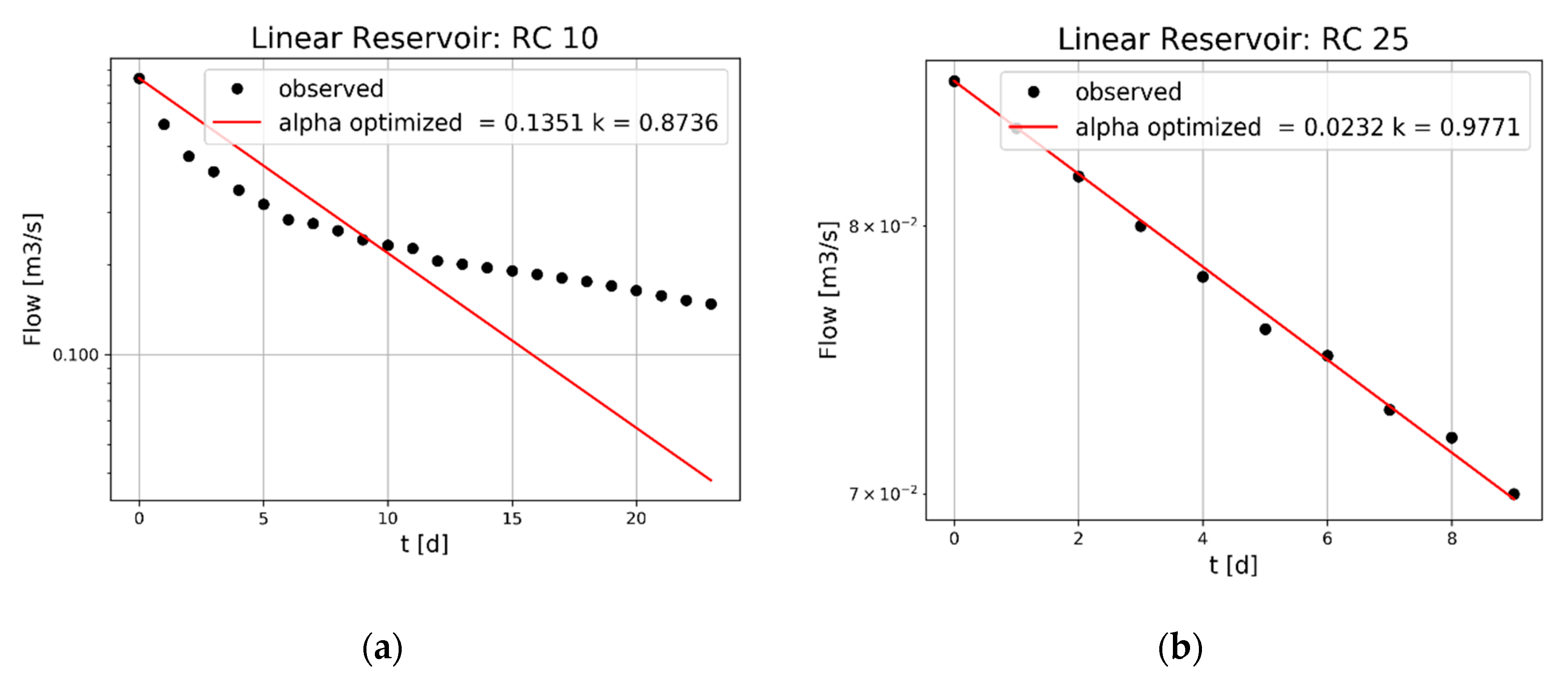
Using the methodology described in Section 2.3.1 for selection, a total of 40 recession periods were identified. Examining the recession curves (RC) in a semilogarithmic plot revealed that a linear approximation is often valid, although there are noticeably convex shaped recessions as well, as shown as an example in Figure 2. Alpha optimized denotes the best fit α according to Equation (2) for the given RC. RC10, which is recession curve number 10, is convex shaped when examined in its entirety. Considering the lower portion of the recession curve, it is nearly linear. This behavior was observed in several other recessions as well. Calculating α and k for this lower section of RC10 yields values of 0.0349 for α and 0.966 for the recession coefficient k. In contrast, RC25 shows linear recession behavior over its entirety.
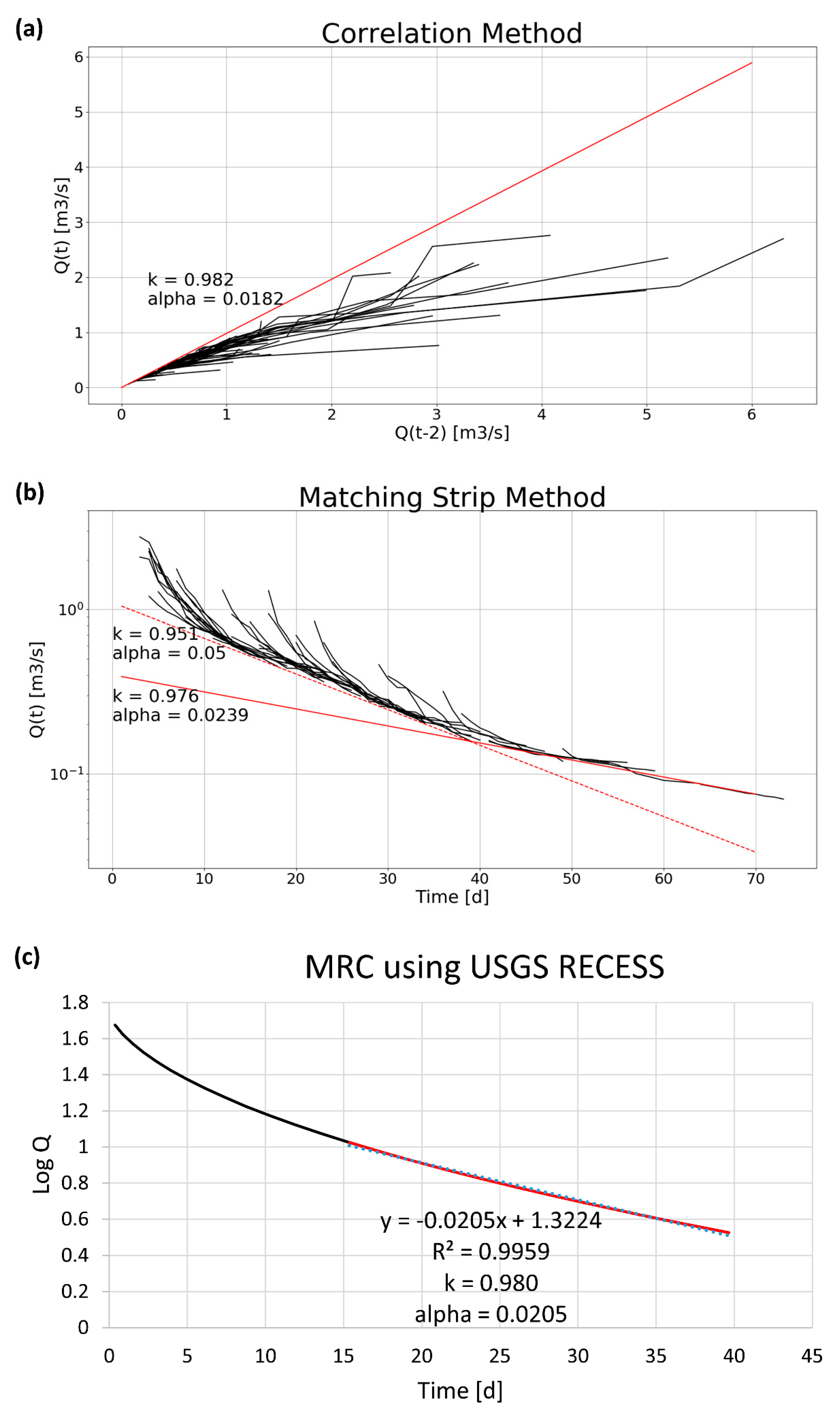
In order to determine a representative value for the recession coefficient k three master recession curves were constructed. The results are depicted in Figure 3. The determined values of k are 0.982, 0.976 and 0.980 for the correlation method, matching strip method and USGS RECESS, respectively. Both the matching strip method and USGS RECESS found that the MRC is somewhat convex shaped, however, nearly linear sections can be identified. The MRC constructed via the matching strip method indicates two baseflow sources may be present. For the faster component, a recession coefficient of 0.951 is determined, whereas for the slower component, the recession coefficient is found to be 0.976. In the USGS RECESS plot, varying the linear approximation from t = 10 to t = 20 as the starting point produces only very minimal changes in k between 0.979 and 0.981. Calculating k over the entire MRC yields k = 0.971. Based on an MRC derived by Michael [49] for the Fischbach catchment during the period 03.2017 to 03.2018, the value for k is found to be 0.971. Nathan and McMahon [7] give typical ranges of the recession coefficient k for different flow components:
- Surface runoff: 0.2–0.8
- Interflow: 0.7–0.94
- Baseflow: 0.93–0.995
The determined recession constants are within the typical range for baseflow. The value (0.976) of k determined via the matching strip method was taken as filter constant in applying the RDF to the data.
3.2. Recession Analysis: Nonlinear Reservoir
The same recession periods used in Section 3.1 were applied in determining the parameters of a nonlinear reservoir. The mean and median of the recession coefficient a are 17.37 and 14.75, respectively. Wittenberg [15] found a significant correlation between catchment size and a when fixing b to a constant value. In the mentioned study b was set to 0.4. For catchments of comparable size to the Fischbach catchment a mean a value between 9 and 14 was found [15]. The determined mean a value in the Fischbach catchment is larger, yet still comparable.
3.3. Recursive Digital Filters and Nonlinear Reservoir Filter
The Chapman and Maxwell filter [20], Eckhardt filter [21] and the nonlinear reservoir filter (NLRF) were applied to the flow data series from 1974 to 2013. The results are listed in Table 1.
The estimates of the BFI differ greatly and range from 25% (Eckhardt filter) to 82% (NLRF). Possible explanations are:
- BFImax is the upper limit of the computed BFI with the Eckhardt filter, consequently higher BFI values are not possible [21]. Furthermore, BFImax = 0.25 as is suggested by Eckhardt [21] is only based on the analysis of three catchments by Kaviany [50]. The BFI values for these catchments were estimated using the Kille method.
- The Chapman and Maxwell filter is not constrained by BFImax. Therefore, a higher BFI value is calculated when compared to the Eckhardt Filter.
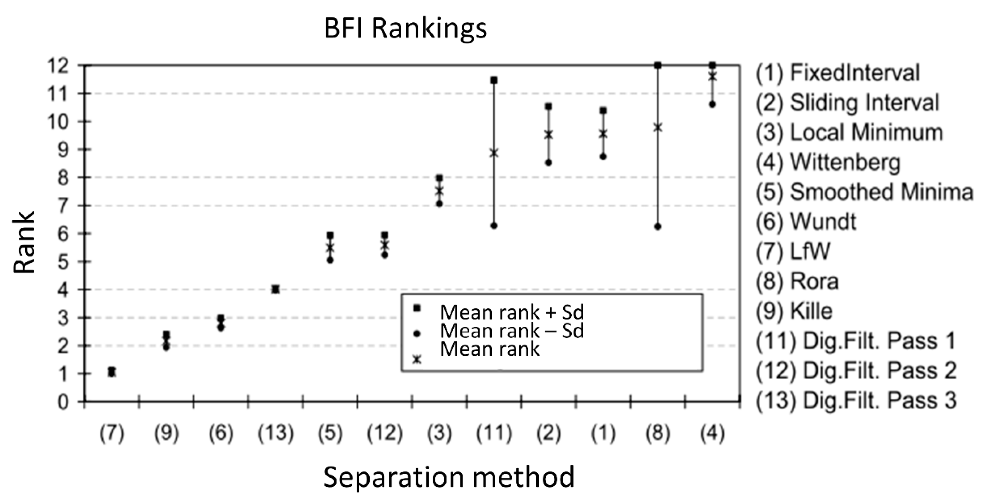
- Filtering via the NLRF generally leads to higher BFI values [16]. Rojanschi [51] compares twelve baseflow separation methods and ranks them by ordering from the lowest (rank = 1) to the highest in computed BFI values. The NLRF, denominated as Wittenberg, is ranked the highest (rank = 12), therefore, it consistently computed higher BFI values than any of the other methods. The Kille method is ranked as determining the second lowest BFI values (r = 2). The ranking of all the considered methods in the comparison by Rojanschi [51] is shown in Figure 4.
The Eckhardt filter with the preset value for BFImax is consequently limited by the BFI value determined via the Kille method, and therefore, when compared to the NLRF large discrepancies in the calculated BFI can be expected.
3.4. Non Continuous Baseflow Estimation Methods
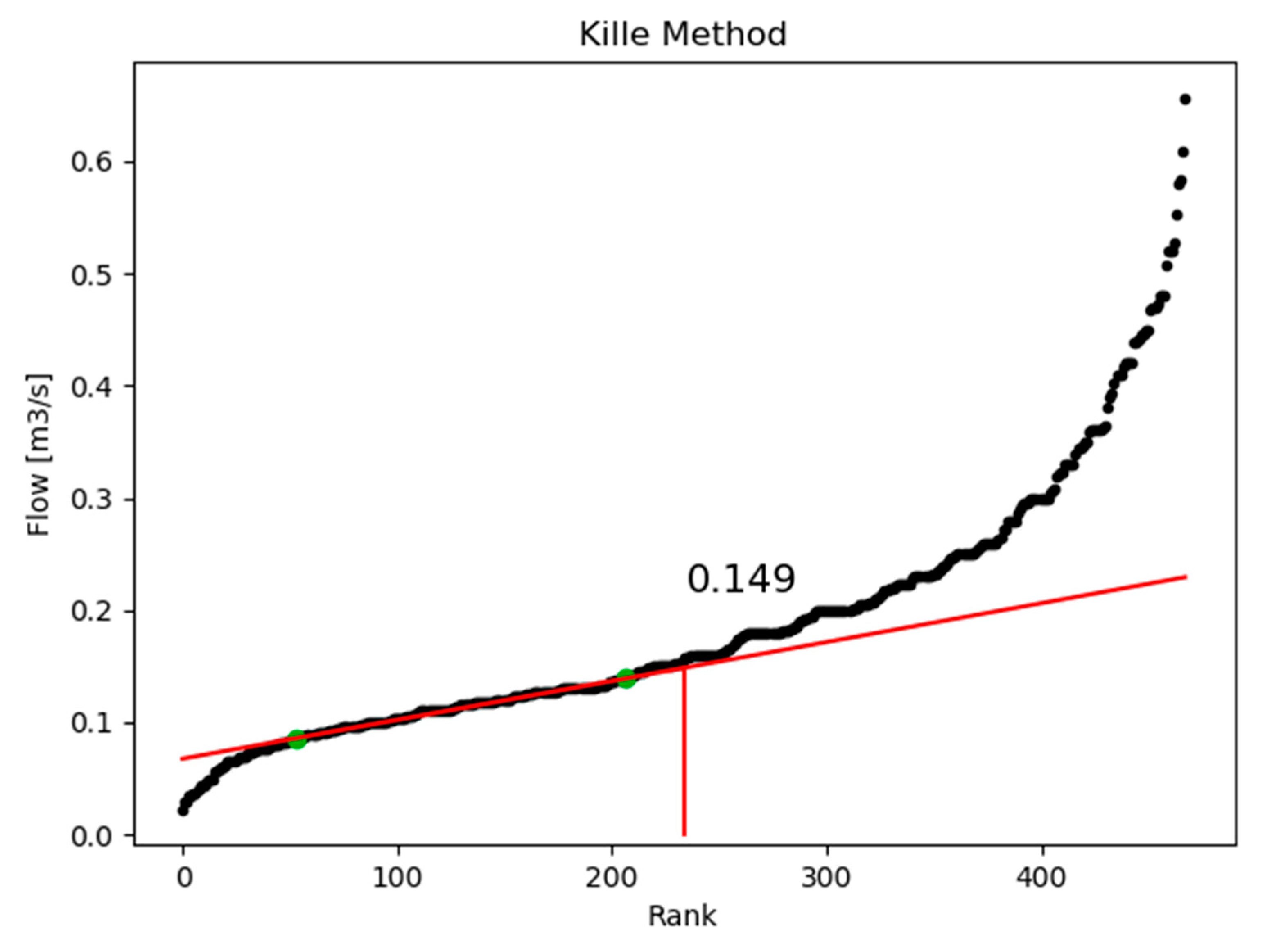
The Kille method and the ratio of Q90/Q50 were applied to determine a mean baseflow estimate. The plot of the ranked monthly minima from 1974 to 2013 is shown in Figure 5. As expected for the considered region, the curve is S-shaped and nearly linear in its mid-section. Mean baseflow is found to be 0.149 m3/s, which corresponds to a BFI of 0.44.
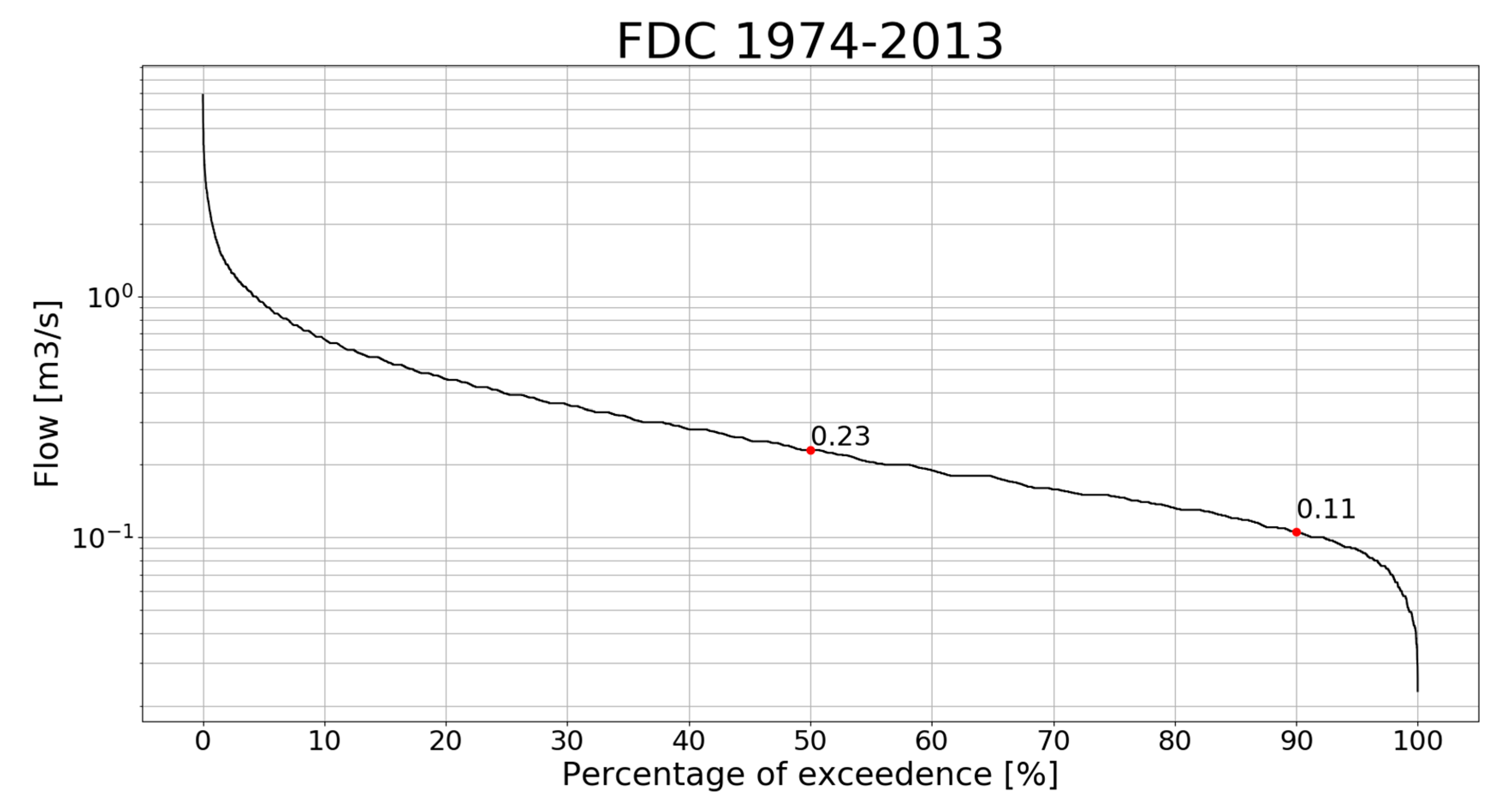
To determine the ratio of Q90/Q50, the FDC was constructed for the same time period as for the other methods. Figure 6 depicts the FDC as well as the values of Q90 and Q50, which were determined to be 0.11 m3/s and 0.23 m3/s, respectively. The ratio gives a BFI of 0.48.
3.5. EC Data Analysis
EC data analysis is split into the analysis of the weekly monitoring and continuous monitoring data.
3.5.1. Weekly Data
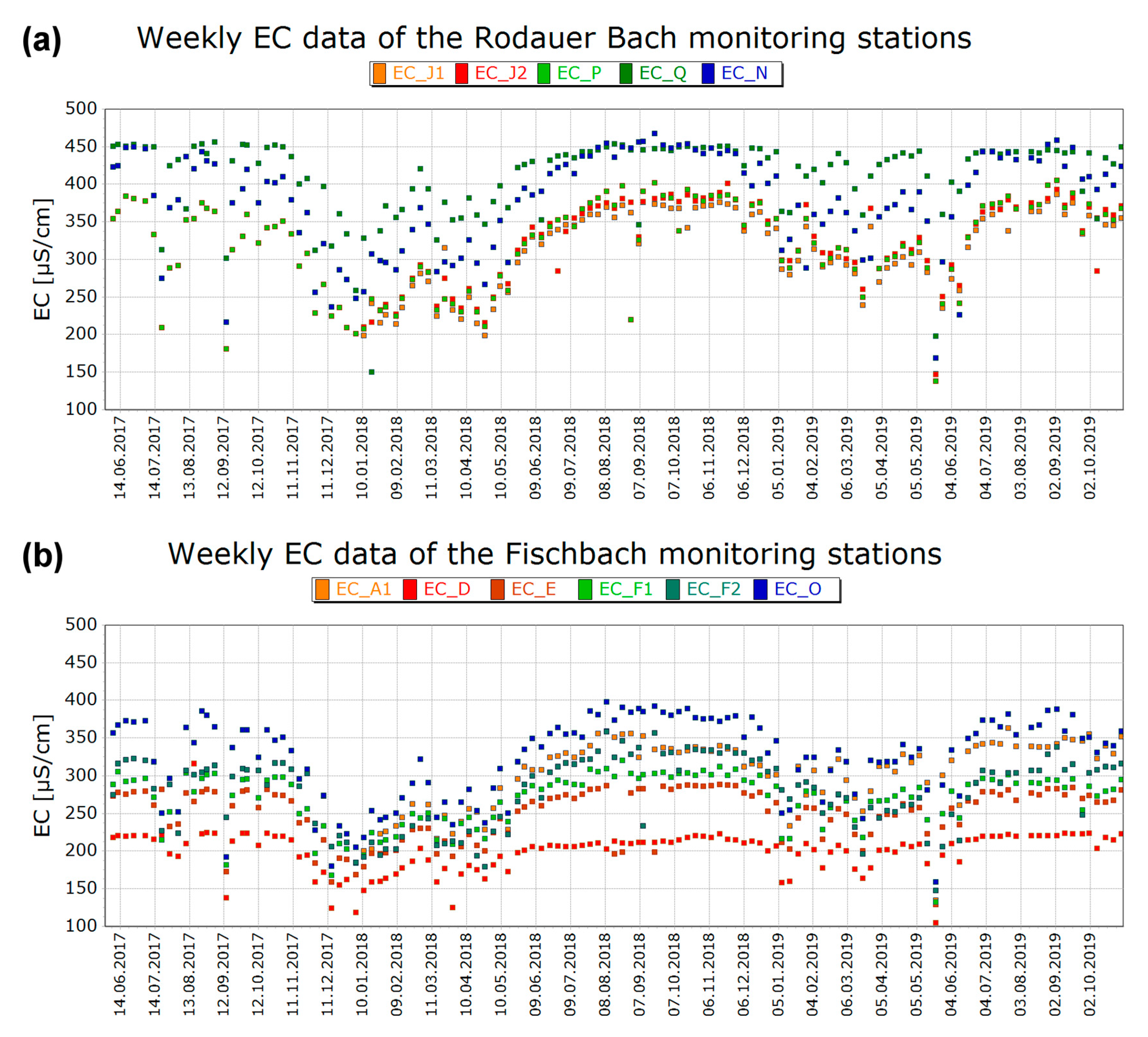
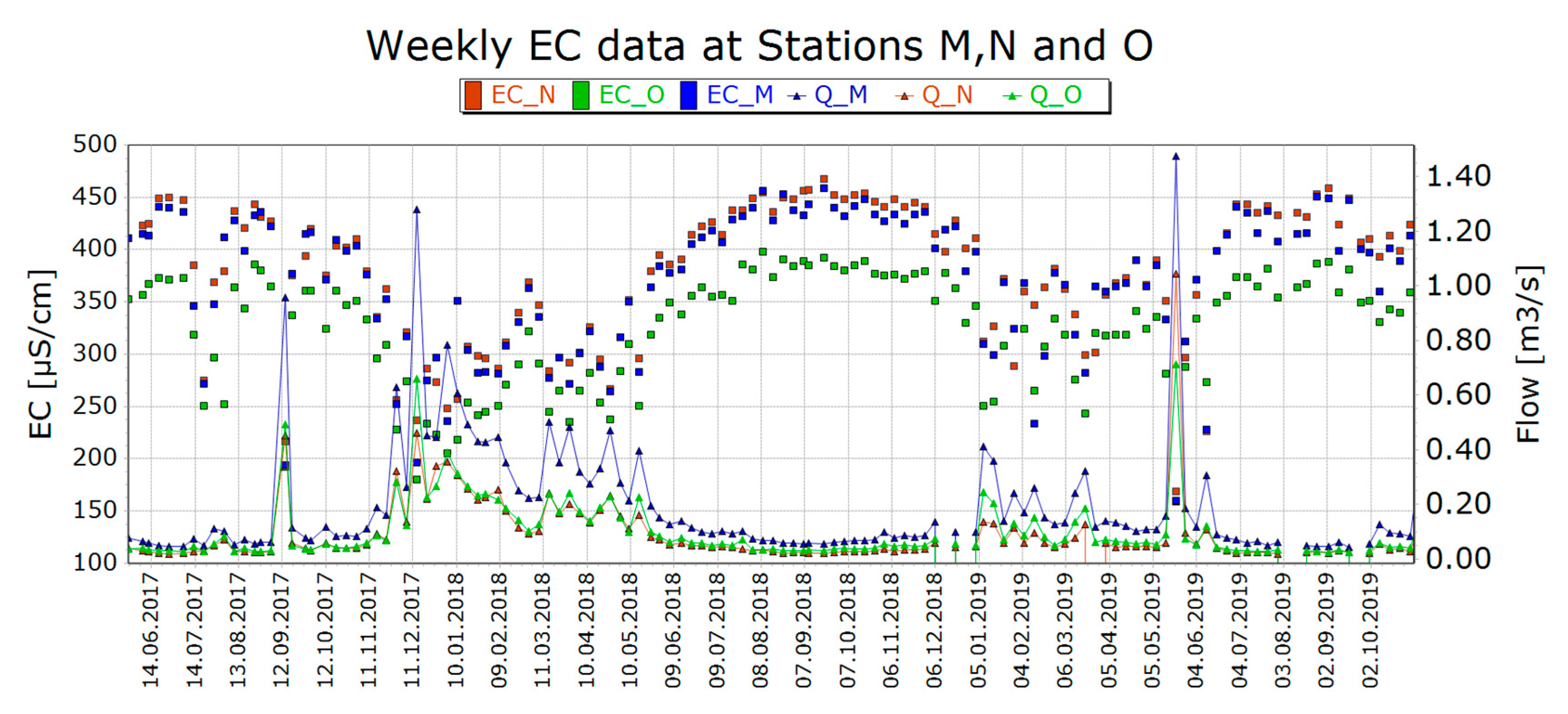
Weekly EC and streamflow measurement data from June 2017 to October 2019 are analyzed at twelve monitoring points in the Fischbach catchment. Schmalz and Kruse [28] note an increase in mean EC from the source region to the gaging station at the catchment outlet and conclude that the total influence of pollution is small due to forests covering roughly 50% of the catchment area, settlements only accounting for 6.5% of the area and no influence through WWTP discharges being present. This increase in EC is apparent in Figure 7 for both the Rodauer Bach and the Fischbach. The stations are sorted from source to outlet. Generally, the registered EC is higher in the branch of the Rodauer Bach than in the Fischbach branch [28]. A seasonal variation in EC is visible in both plots. Higher EC values are registered during the dryer conditions in the summer months and lower EC values during wetter conditions in winter and spring months. EC values during the summer months (June to August) tend to plateau at about 450 µS/cm at station N and at about 380 µS/cm at station O. The lowest EC values are recorded either during the winter and springs months (November to May) with generally higher flows. The lowest recorded EC at station N is about 240 µS/cm during winter and about 170 µS/cm during spring. At station O the lowest values of about 170 µS/cm and 160 µS/cm were registered for winter and spring. Figure 8 depicts the EC and flow at stations O and N as well as after the Rodauer Bach flows into the Fischbach, as recorded further downstream at station M at the catchment outlet. As to be expected, registered EC values at station M lie between those at stations N and O. During the summer months, EC at station M plateaus at about 430 to 450 µS/cm and reaches its lowest values of about 200 µS/cm and 160 µS/cm during winter and spring, respectively. Table 2 contains the mean and median of measured EC values at each monitoring point in the Fischbach catchment.
3.5.2. Continuous Data
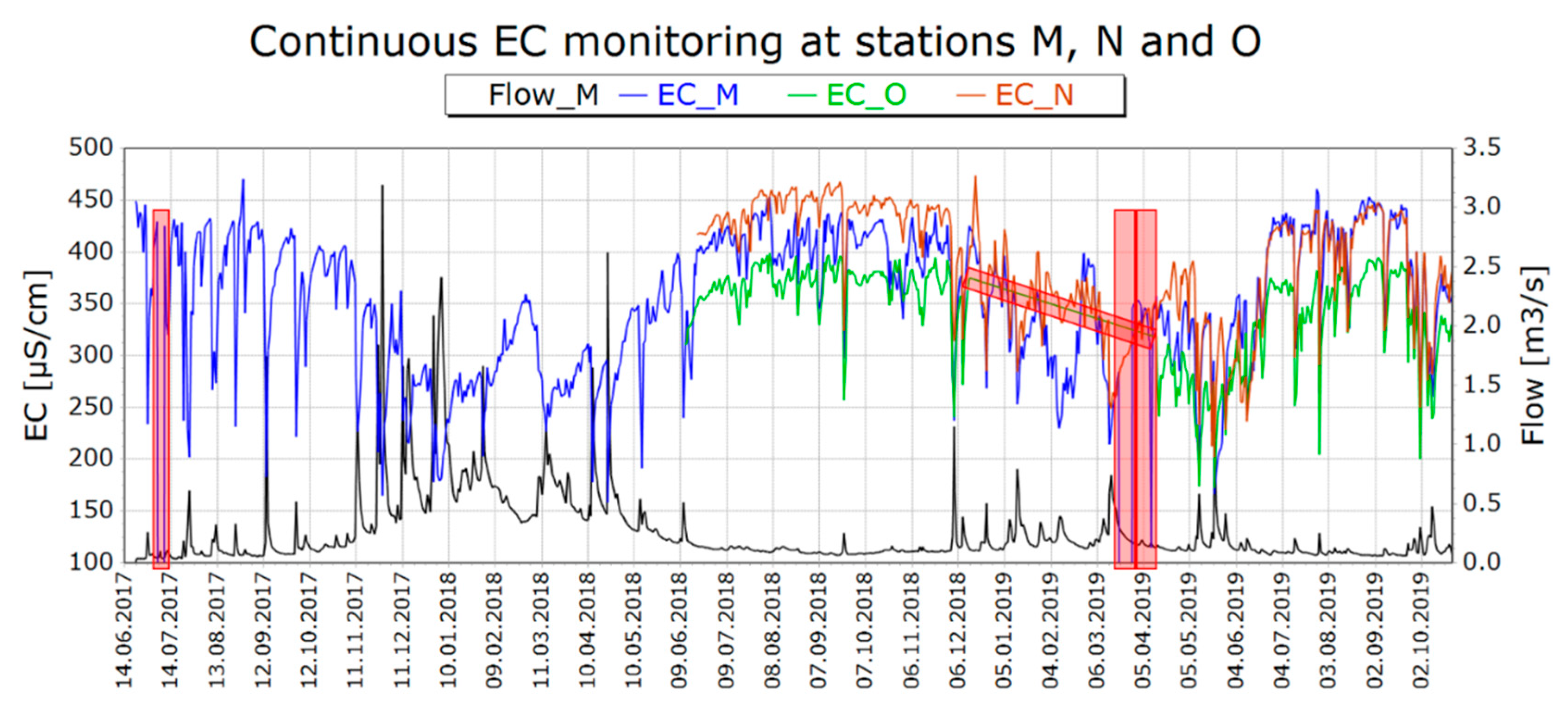
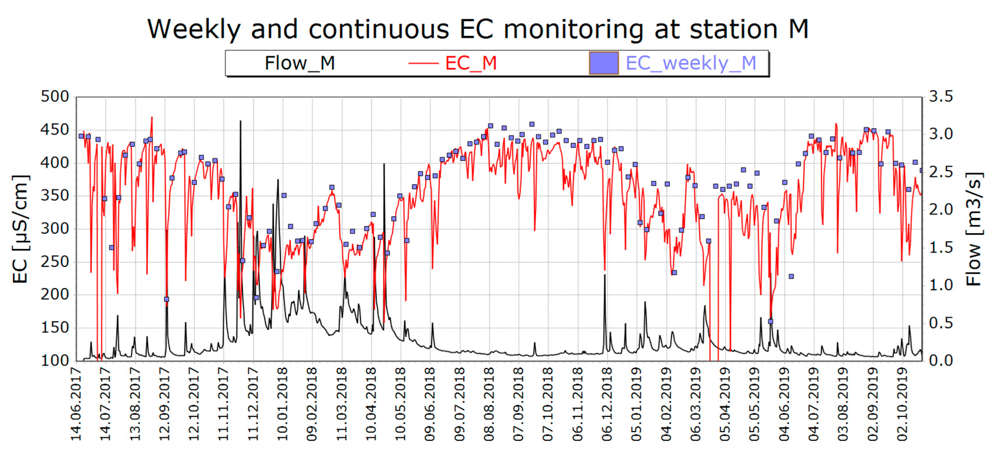
Continuous EC monitoring has been conducted at station M since June 2017 and since June 2018 at stations N and O as well. The daily EC data at stations M, N and O as well as the daily flow data at station M are shown in Figure 9. As with the weekly data, the EC values at M lie between those at N and O. In the summer of 2019, EC at M is closer to EC at N. While in the summer of 2018, flow at O was higher than at N; the flows are nearly identical in the summer of 2019. This is likely due to 2018 being a very dry year with only about 71% of the average precipitation for the federal state of Hesse [52]. Consequently, the groundwater aquifers were more drained at the end of 2018 and not replenished to levels before 2018 by the summer of 2019. Seasonal variation within the EC record is visible, as is the case with the weekly data. Higher EC values are registered during the summer and lower values during the winter/spring. The plateaus reached during the low flow periods in summer are comparable to those identified with the weekly EC data. The lowest EC values are found to be about 160 µS/cm, 200 µS/cm and 175 µS/cm at station M, N and O, respectively. It should be noted that the lowest EC value at M was measured before continuous observations at N and O were available. Overall weekly EC monitoring values and average daily EC values match quite well (Figure 10). However, the weekly monitoring EC values are measured only once in the morning during a monitoring day, whereas the daily mean EC values are calculated based on continuous monitoring. This leads to weekly and continuous monitoring EC values not matching exactly.
3.6. Mass Balance Filtering
Based on the suggestions of Stewart et al. [27], the values for ECbaseflow and ECrunoff were determined during low flow conditions and during wet and/or high flow periods, respectively. EC in precipitation was measured for a single rainfall event in September 2018 and was found to be 5 µS/cm.
3.6.1. Estimation of ECbaseflow
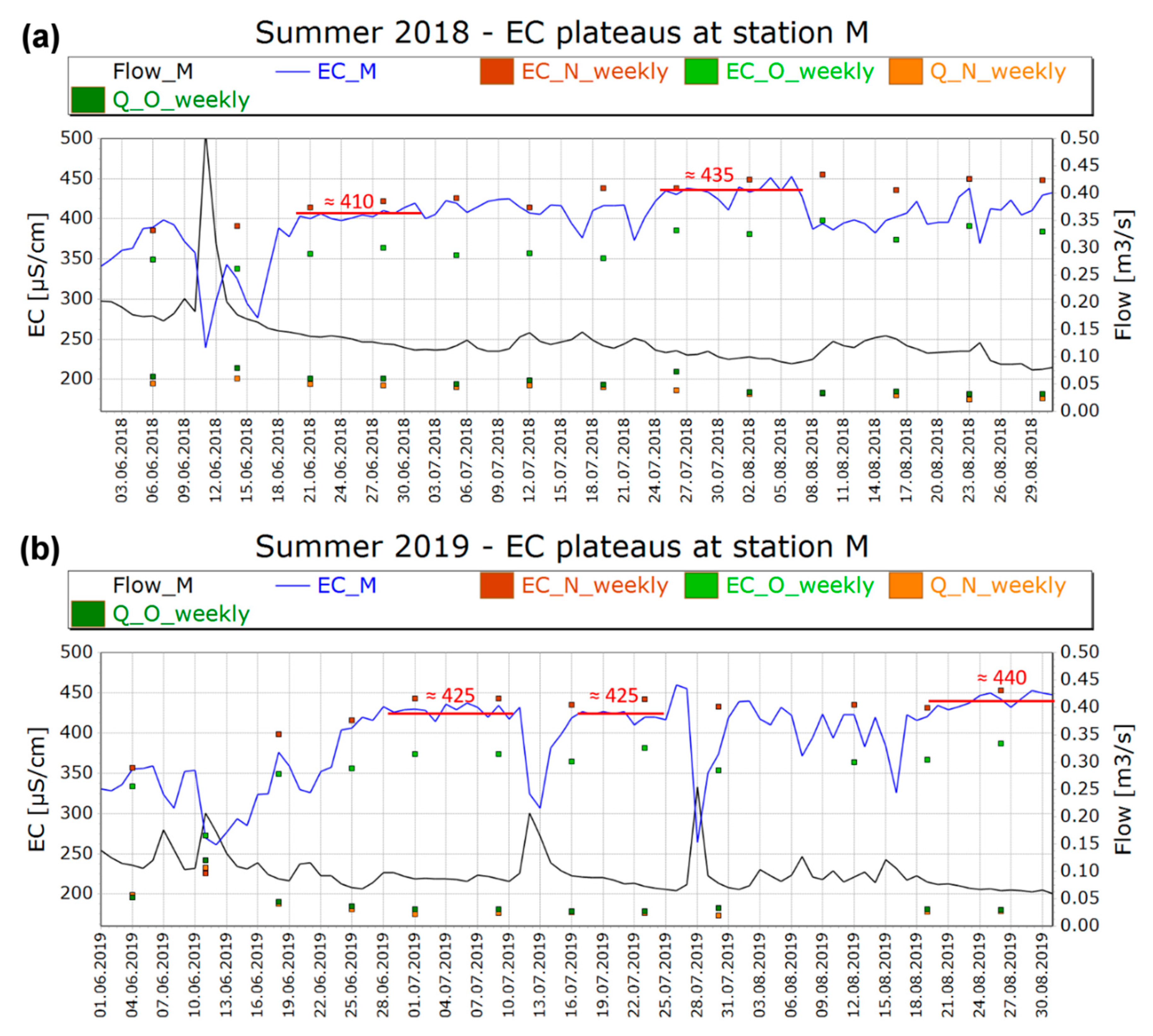
Low flow conditions in the considered region are typically in the summer months when the evapotranspiration is high. ECbaseflow was estimated for the summer of 2018 and 2019 in order to examine if the estimates would remain relatively constant. The EC and flow during these periods are shown in Figure 11. For the summer of 2018, ECbaseflow is estimated to be between 410 and 435 µS/cm when determined using the daily EC values registered as station M. The estimate for the summer of 2019 is between 425 and 440 µS/cm. The estimate of ECbaseflow therefore remains relatively constant. The mean and median EC for summer 2018 are 399 µS/cm and 406 µS/cm, respectively. For the summer of 2019, the mean EC is found to be 393 µS/cm and the median EC is 418 µS/cm. Using the weekly EC data at station M yields an estimate of 430–450 µS/cm for ECbaseflow (see Section 3.5.1.). For use in the MBF, the ECbaseflow is set to 450 µS/cm.
It can be concluded that weekly EC measurements can be sufficient to estimate ECbaseflow, given that an appropriate period during the year is chosen in which low flow conditions are typical. For the German low mountain range, the summer months (June–August) are found to be the time period in which ECbaseflow can be estimated consistently. Based on Figure 8 and 10, September can be suitable as well. Therefore, measurement campaigns should span a minimum of three months. Li et al. [53] concluded that a minimum of two months is necessary for estimating a stable ECbaseflow value for a catchment in Canada.
3.6.2. Estimation of ECrunoff
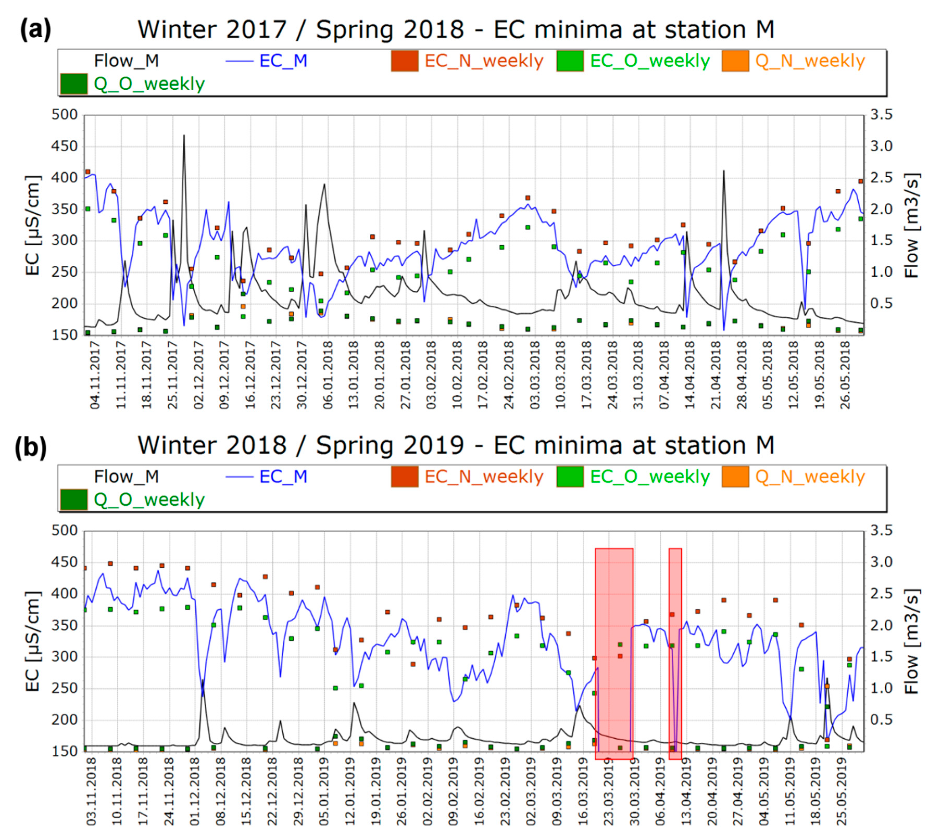
The winter and spring months were considered to estimate ECrunoff. The winter/spring of 2017/2018 as well as 2018/2019 are considered individually (Figure 12). ECrunoff is estimated as the minimum registered EC value at station M. For the winter/spring period of 2017/2018, minimum EC is about 160 µS/cm. The range of the EC minima at peak flow values is 160–230 µS/cm. However, when considering individual and distinct flow peaks above 2.0 m3/s, the range is about 160–180µS/cm. Peak flows are much lower in the winter/spring period 2018/2019 with a maximum peak flow of about 1.2 m3/s, whereas the maximum peak flow in the previous period was approximately 3.2 m3/s. Nonetheless, a similar range in EC minima can be found with values from 170 to 230 µS/cm. Unlike for the previous winter/spring period a cutoff flow value at which the EC minima range is narrower cannot be found, yet the absolute registered EC minima are very similar with 160 µS/cm and 170 µS/cm for 2017/2018 and 2018/2019, respectively. Therefore, it is assumed that ECrunoff as minimum EC can be considered relatively constant. Considering weekly EC data, the lowest EC values of about 200 µS/cm and 160 µS/cm are determined during winter/spring 2017/2018 and 2018/2019, respectively (see Section 3.5.1). ECrunoff is set to 150 µS/cm for the MBF.
Weekly monitoring can lead to roughly equivalent estimates, however, true minimum values may be missed depending on the time of peak flow and when sampling is done. For the German low mountain range, the time period of winter and spring regarding a hydrological winter half year (November to April) as well as May is found to be appropriate to estimate ECrunoff as conditions are typically wetter. Accordingly, a minimum of seven months should be planned for measurement campaigns to estimate ECrunoff. Li et al. [53] concluded that a minimum of six months is necessary.
3.6.3. Mass Balance Filtering Using EC
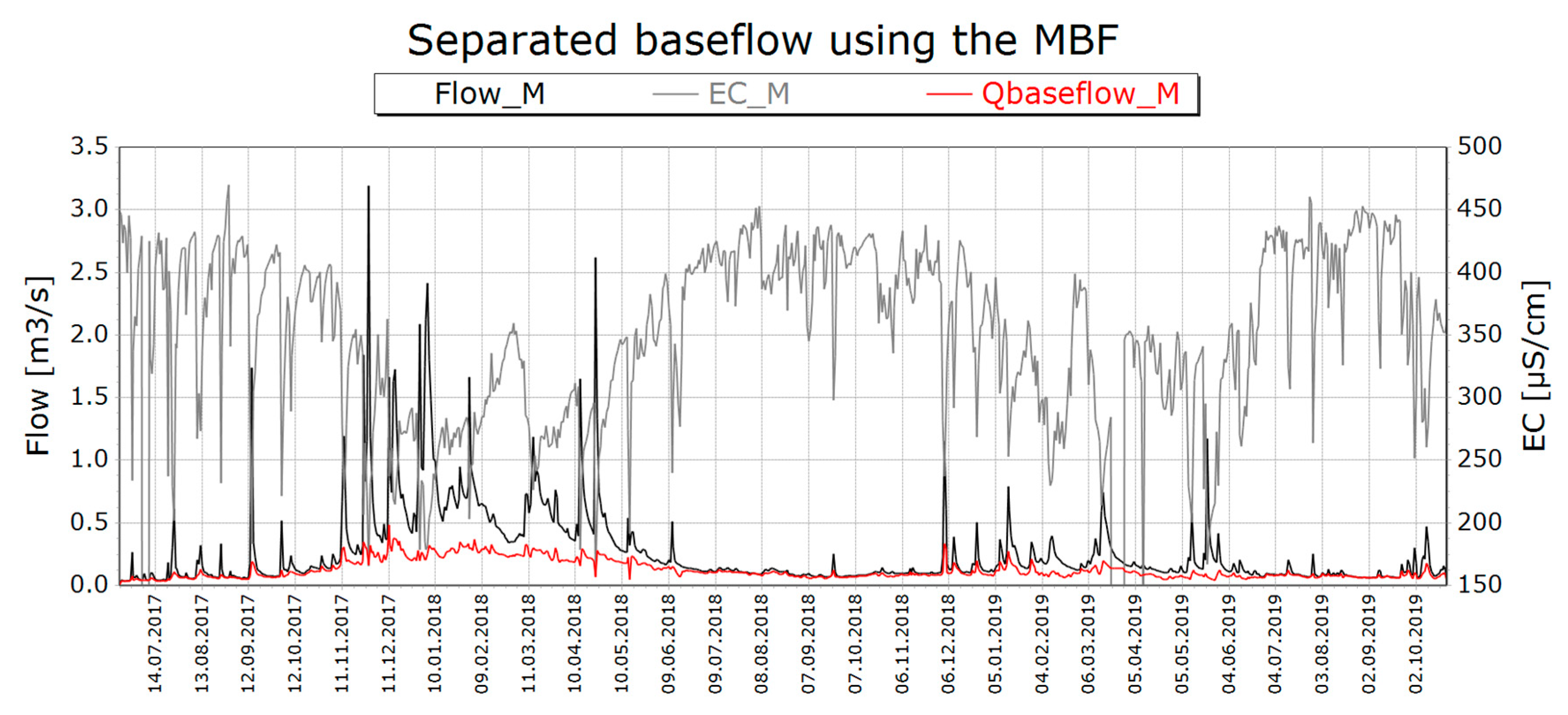
Applying the MBF with ECbaseflow and ECrunoff values as given in Section 3.6.1 and Section 3.6.2 yields a BFI of 0.47. The separated baseflow as well as total observed flow and EC are shown in Figure 13.
4. Discussion
4.1. Discussion on Data Availability and Requirements
Flow data from 1974 to 2019 from the HLNUG as well as high resolution water level and EC data from the ihwb as of June 2017 was available for this study. Recession analysis was conducted using HLNUG flow data from 1974 to 2013, as it was conducted before verified and corrected data were available for the time after 2013. According to Tallaksen [12], Perzyna [54] found that a minimum of 10 years is necessary to reliably estimate the recession coefficients. The same minimum time span is suggested for the Kille method as well [43]. The recession constant k used in the RDFs was determined to be 0.976 and is well within the typical range for baseflow recessions. All considered methods for constructing an MRC and estimating k gave similar estimates) see Section 3.1.). The estimated mean recession constant a of the NLRF was found to be 17.37 and is slightly larger than the a values estimated by Wittenberg [15] for catchments of similar size (see Section 3.2.).
Additionally to the long-term daily data from the HLNUG, high resolution data of EC and water level and weekly monitoring data were available as well for a time span of two years and three months at station M at the Fischbach catchment outlet. At stations N and O high resolution data was available as of June 2018 for a time span of 14 months. Li et al. [53] found that a minimum of six months of EC sampling for a reliable estimation of ECrunoff and two months of sampling for the estimation of ECbaseflow is necessary. In the aforementioned study, a dataset of 19 years was available for statistical analysis. The considered dataset in this study is much shorter but still four times longer than the minimum requirement of six months for the estimation of ECrunoff. Consequently, rather than a statistical analysis, an estimate of the minimum sampling duration was made by considering the typical low flow and high flow periods within the German low mountain range. According to the HLNUG [52], the lowest flows are in the months June to September. Considering the continuous EC data in these months for both 2018 and 2019 showed that EC plateaus remained relatively constant with an EC of 410–440 µS/cm. Using the weekly EC data, the plateaus were found to be between 430 and 450 µS/cm. It can be concluded that continuous and weekly monitoring data within the months of June toAugust and, depending on precipitation, September can be used to estimate ECbaseflow in the German low mountain region. The months November to May were considered for the estimation of ECrunoff. Longobardi et al. [25] found that the highest EC values were registered during the summer and autumn months in a Mediterranean catchment, whereas the lowest were found during the winter and spring months. For the winter and spring period of 2017/2018 a cutoff value of 2 m3/s was found at which EC minima remained relatively constant between 160 and 180 µS/cm. The winter and spring period of 2018/2019 had considerably lower flows and a cutoff peak flow, after which a relatively constant EC minimum was reached, could not be found. However, the absolute minimum EC value in this period was within the range found for 2017/2018. Weekly monitoring data indicated an ECrunoff range between 160 and 200 µS/cm. Weekly monitoring can lead to similar estimates, however, it must be considered that this is a sample taken once during a monitoring day. If sampling does not coincide well with peak flow, the EC measurement may not be representative for the actual EC minimum. A longer monitoring period is needed for both continuous and weekly EC monitoring in order to estimate ECrunoff reliably as variability is greater due to high flows being dependent on precipitation. Li et al. [53] noted the higher variability in ECrunoff as well. The results indicate a minimum of seven months sampling duration for estimation of ECrunoff. Both 2018 and 2019 were dry years. The winter of 2017/2018 however was rather wet [52]. Therefore, 2018 was especially suited to analyze EC based on the typical flow regime within the German low mountain range as the high and low flow periods were very distinct. The year 2019 is more difficult in this respect. While the summer months showed pronounced low flow periods as well, the winter and spring of 2018/2019 had significantly lower flows. This can be attributed to groundwater levels being low at the end of 2018 due to the hot and dry summer of 2018. The precipitation in the following winter was not sufficient to elevate ground water levels to their typical levels [52]. The estimated ECrunoff could consequently be biased by low antecedent precipitation and low ground water levels if the duration of a monitoring campaign is too short. ECbaseflow could potentially be estimated during winter and spring months if conditions are similar to the conditions described for 2018/2019 (Figure 12b). If more typical conditions are prevalent, ECbaseflow is best estimated during the summer months.
4.2. Discussion on Application and Validity of Baseflow Separation Methods
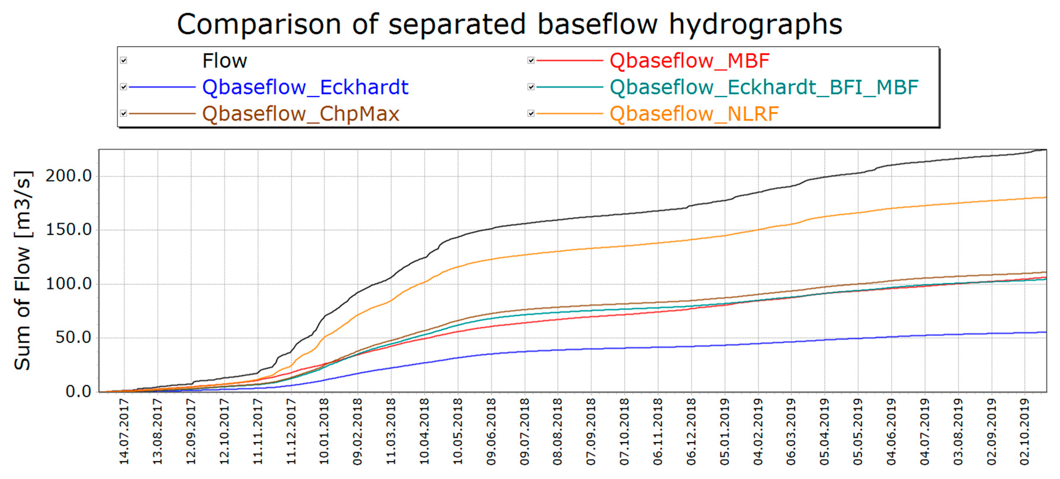
The results of all the applied baseflow separation methods and BFI values determined from literature, as well as the considered time periods, are compiled in Table 3. The mean estimated BFI value is 0.49 ± 0.18. The relatively large standard deviation of ±0.18 is due to the significantly different results of the Eckhardt filter and the NLRF compared to the other methods. The other four methods are all within the range of 0.44–0.50 regarding estimated BFI. Therefore, the Kille method, FDC Q90/Q50 ratio and the Chapman and Maxwell filter estimated BFI values very close to the BFI value determined via the MBF. The BFI for all the methods was additionally estimated for the time period 06.2017–10.2019—the reference period for the MBF. The varied time frame only resulted in minor differences (Table 3). Setting BFImax to the BFI value determined via the MBF (0.47) results in an estimated BFI of 0.46 using the Eckhardt filter. When the cumulative sum of baseflow is inspected (Figure 14), the Chapman and Maxwell filter as well as the Eckhardt filter using the adjusted BFImax value follow the cumulative sum of the MBF the closest. These methods could be calibrated further by adjusting the filter constant a and/or BFImax to the results of the MBF and could be used to separate baseflow hydrographs in time periods without available EC data and still produce comparable results. Okello et al. [5], Lott et al. [4] and Gonzales et al. [40] found that the Eckhardt filter can be calibrated using tracer data to estimate reliable BFI values as well.
In this study the preset value of BFImax according to Eckhardt [21] for perennial rivers with hard rock aquifers is found to be too low for the considered region. The preset BFImax value is similar to the BFI value found using the mean yearly low flow in the Fischbach catchment (Table 3). Several estimated BFI values were found in the literature or calculated using data from the literature regarding either the Fischbach catchment or the crystalline Odenwald region in general and are listed in Table 3. The BFI values range from 0.28 to 0.57 and are consistent with the findings in this study. The calculated BFI using the mean yearly low flow as given in the HLNUG [31] is considered to be a reasonably quick and easy first estimate when data is available. However, it underestimates baseflow, as the mean yearly low flow is calculated as the mean of the lowest recorded flow of each year and therefore only represents the driest conditions within a catchment and does not consider higher baseflow contributions during wet periods. The HLNUG [30] considered low flow measurements taken throughout the federal state of Hesse in September 2004 and came to a similar conclusion, albeit using individual measurements during low flow conditions rather than the long mean yearly low flow. Both the estimated BFI from the HLNUG [30,55] are very close to the MBF estimated BFI. The BFI estimated by Michael [49] is based on a single year from March 2017 to March 2018. The time period for which EC data is available does not match. However, two complete hydrological years, 2018 and 2019, are part of the time period for which EC data is available. The BFI values for each individual hydrological year are given in Table 4. The Kille method and the FDC Q90/Q50 ratio are excluded from this analysis as individual hydrological years are analyzed. Comparing the BFI values of the hydrological years and the BFI value determined by Michael [49], it can be concluded that they are within a similar range. The Chapman and Maxwell filter and the Eckhardt filter with adjusted BFImax are within a reasonable range when compared to the MBF regarding estimated BFI for individual hydrological years. Interestingly, all filter methods estimate higher BFI values for 2018 and lower for 2019 except for the MBF. This is most likely due to 2018 having had a wet winter/spring period (November 2017 to May 2018) whereas 2019 did not. This can be seen in Figure 14 where the slopes of the cumulative sums of baseflow are steeper when compared to the MBF during the winter/spring of 2018, indicating that a higher baseflow was separated during this period. Accordingly, a higher BFI is estimated for 2018 than for 2019. The higher BFI estimated by the MBF for 2019 is due to the slope of total observed flow and separated baseflow being rather similar, indicating that the direct runoff component is smaller. Overall, the application of an MBF within the German low mountain range is feasible using continuous as well as weekly EC monitoring to estimate the flow components. The BFI values estimated via the MBF are within the range of values found in the literature and comparable to those of other applied methods.
5. Conclusions
In this study the baseflow in the Fischbach low mountain range catchment has been analyzed. The objectives of this study were to (I) compile and analyze already existing and newly measured data to determine a plausible baseflow estimate for the new research basin, (II) examine the use of EC for mass balance filtering in the German low mountain range and (III) compare different types of baseflow separation methods and identify suitable methods for the German low mountain range.
Long term daily flow data was used for recession analysis and application of the RDFs, NLRF, as well as the Kille method and the FDC Q90/Q50 ratio. A mass balance filter was applied using high resolution EC and water level measurements resampled to daily values.
In order to apply the MBF, the parameters ECbaseflow and ECrunoff needed to be estimated. Regarding measurements to estimate ECbaseflow, the summer months from June to August as well as September were found to be suitable. Both continuous and weekly monitoring can be used to estimate ECbaseflow with estimates ranging between 425–440 µS/cm and 430–450 µS/cm, respectively. ECrunoff can be estimated during the winter and spring months from November to May. Weekly monitoring can result in similar estimates compared to continuous monitoring; however, at minimum, a full winter and spring period should be monitored, and if possible, measurements should be taken during high flow periods.
Of the applied methods, the Kille method, FDC Q90/Q50 ratio, the Chapman and Maxwell filter as well as the Eckhardt filter with adjusted BFImax produced results similar to the MBF. The estimated BFI value using the MBF is consistent with BFI values found in the literature.
Estimated BFI values for the Fischbach catchment can be used in ongoing research at the ihwb (Chair of Engineering Hydrology and Water Management) of the Technical University of Darmstadt. These research topics include hydrological modelling activities, process-oriented measurement campaigns and climate scenario analysis for the Fischbach and Gersprenz catchments.
The Gersprenz catchment, which the Fischbach catchment is a part of, was chosen as a field observatory by the ihwb as it is a representative study area for the German low mountain range [28]. Therefore, the results of this study are useful for similar studies within the same region, as they are based on long-term daily as well as high resolution data, local knowledge and hydrological process understanding in the Fischbach catchment.
For further studies in low mountain range regions, we recommend using an ensemble of methods. The FDC Q90/Q50 and the Kille method provide a quick and easy mean baseflow estimate. However, if a continuous baseflow estimate is required, the Chapman and Maxwell filter as well as the Eckhardt filter are found to be adequate methods. The Eckhardt filter’s BFImax parameter should however be calibrated using either results from the MBF or using the BFI estimated via the FDC Q90/Q50 or Kille method. For the MBF, weekly and continuous monitoring was found to be adequate to estimate necessary parameters. It was found that monitoring should be conducted for a minimum duration of three months for ECbaseflow and seven months for ECrunoff.
Author Contributions
Conceptualization, M.K. and B.S.; data curation, M.K. and B.S.; investigation, M.K.; methodology, M.K. and B.S.; software, M.K.; supervision, B.S.; visualization, M.K.; writing—original draft, M.K.; writing—review and editing, B.S. All authors have read and agreed to the published version of the manuscript.
Funding
This research received no external funding.
Acknowledgments
The authors would like to thank the HLNUG, RP Darmstadt and the Wasserverband Gersprenzgebiet for making data available and allowing installation of equipment for the monitoring campaigns.
Conflicts of Interest
The authors declare no conflict of interest.
References
- Klimaveränderung, U. Wasserwirtschaft (KLIWA) Das Jahr 2018 im Zeichen des Klimawandels? Viel Wärme, wenig Wasser in Süddeutschland. 2019, p. 14. Available online: https://www.kliwa.de/_download/Rueckblick2018.pdf (accessed on 22 April 2020).
- Kopp, B.; Baumeister, C.; Gudera, T.; Hergesell, M.; Kampf, J.; Morhard, A.; Neumann, J. Entwicklung von Bodenwasserhaushalt und Grundwasserneubildung in Baden-Württemberg, Bayern, Rheinland-Pfalz und Hessen von 1951 bis 2015. Hydrol. Wasserbewirtsch. 2018, 62, 62–76. [Google Scholar]
- Klaus, J.; McDonnell, J.J. Hydrograph separation using stable isotopes: Review and evaluation. J. Hydrol. 2013, 505, 47–64. [Google Scholar] [CrossRef]
- Lott, D.A.; Stewart, M.T. Base flow separation: A comparison of analytical and mass balance methods. J. Hydrol. 2016, 535, 525–533. [Google Scholar] [CrossRef]
- Okello, S.L.; Lopes, A.M.; Uhlenbrook, S.; Jewitt, G.P.W.; Masih, I.; Riddell, E.S.; Van der Zaag, P. Hydrograph separation using tracers and digital filters to quantify runoff components in a semi-arid mesoscale catchment. Hydrol. Process. 2018, 32, 1334–1350. [Google Scholar] [CrossRef]
- Natermann, E. Die Linie des langfristigen Grundwassers (AuL) und die Trockenwetter-Abflußlinie (TWL). Wawi 1951, 41, 12–14. [Google Scholar]
- Nathan, R.J.; McMahon, T.A. Evaluation of automated techniques for base flow and recession analyses. Water Resour. Res. 1990, 26, 1465–1473. [Google Scholar] [CrossRef]
- Sloto, R.A.; Crouse, M.Y. HYSEP: A Computer Program for Streamflow Hydrograph Separation and Analysis; Water-Resources Investigations Report 96-4040; U.S. Department of the Interior: Lemoyne, PA, USA, 1996; p. 46.
- Chapman, T. A comparison of algorithms for stream flow recession and baseflow separation. Hydrol. Process. 1999, 13, 701–714. [Google Scholar] [CrossRef]
- Furey, P.R.; Gupta, V.K. A physically based filter for separating base flow from streamflow time series. Water Resour. Res. 2001, 37, 2709–2722. [Google Scholar] [CrossRef] [Green Version]
- Stewart, M.K. Promising new baseflow separation and recession analysis methods applied to streamflow at Glendhu Catchment, New Zealand. Hydrol. Earth Syst. Sci. 2015, 19, 2587–2603. [Google Scholar] [CrossRef] [Green Version]
- Tallaksen, L.M. A review of baseflow recession analysis. J. Hydrol. 1995, 165, 349–370. [Google Scholar] [CrossRef]
- Datta, A.R.; Bolisetti, B.T.; Balachandar, R. Automated Linear and Nonlinear Reservoir Approaches for Estimating Annual Base Flow. J. Hydrol. Eng. 2012, 17, 554–564. [Google Scholar] [CrossRef]
- Millares, A.; Polo, M.J.; Losada, M.A. The hydrological response of baseflow in fractured mountain areas. Hydrol. Earth Syst. Sci. 2009, 13, 1261–1271. [Google Scholar] [CrossRef]
- Wittenberg, H. Nonlinear analysis of flow recession curves. IAHS Publ.-Ser. Proc. Rep.-Int. Assoc. Hydrol. Sci. 1994, 221, 61–68. [Google Scholar]
- Wittenberg, H. Baseflow recession and recharge as nonlinear storage processes. Hydrol. Process. 1999, 13, 715–726. [Google Scholar] [CrossRef]
- Van Dijk, A.I.J.M. Climate and terrain factors explaining streamflow response and recession in Australian catchments. Hydrol. Earth Syst. Sci. 2010, 14, 159–169. [Google Scholar] [CrossRef] [Green Version]
- Wittenberg, H.; Aksoy, H.; Miegel, K. Der schnelle Anstieg des Grundwassers nach Starkregen. Hydrol. Wasserbewirtsch. 2020, 64, 66–74. [Google Scholar]
- Arnold, J.G.; Allen, P.M.; Muttiah, R.; Bernhardt, G. Automated Base Flow Separation and Recession Analysis Techniques. Groundwater 1995, 33, 1010–1018. [Google Scholar] [CrossRef]
- Chapman, T.; Maxwell, A. Baseflow separation-comparison of numerical methods with tracer experiments. In Hydrology and Water Resources 23. Symposium 1996, Proceedings of the Hydrology and Water Recouces Symposium 1996: Water and the Environment, Barton, Australia, 1996; Preprints of Papers; National Conference Publication Institution of Engineers: Barton, Australia, 1996; Volume 96/05, pp. 539–545. [Google Scholar]
- Eckhardt, K. How to construct recursive digital filters for baseflow separation. Hydrol. Process. 2005, 19, 507–515. [Google Scholar] [CrossRef]
- Lyne, V.D.; Hollick, M. Stochastic time-variable rainfall runoff modelling. In Hydrology and Water Resources 24. Symposium 1997, Proceedings of the Hydrology and Water Resources Symposium 1997, Perth, Australia, 10.-12.09.1979; Preprints of Papers; National Conference Publication Institution of Engineers: Barton, Australia, 1997; Volume 97, pp. 89–92. [Google Scholar]
- Aksoy, H.; Kurt, I.; Eris, E. Filtered smoothed minima baseflow separation method. J. Hydrol. 2009, 372, 94–101. [Google Scholar] [CrossRef]
- Mei, Y.; Anagnostou, E.N. A hydrograph separation method based on information from rainfall and runoff records. J. Hydrol. 2015, 523, 636–649. [Google Scholar] [CrossRef]
- Longobardi, A.; Villani, P.; Guida, D.; Cuomo, A. Hydro-geo-chemical streamflow analysis as a support for digital hydrograph filtering in a small, rainfall dominated, sandstone watershed. J. Hydrol. 2016, 539, 177–187. [Google Scholar] [CrossRef]
- Pinder, G.F.; Jones, J.F. Determination of the ground-water component of peak discharge from the chemistry of total runoff. Water Resour. Res. 1969, 5, 438–445. [Google Scholar] [CrossRef]
- Stewart, M.; Cimino, J.; Ross, M. Calibration of Base Flow Separation Methods with Streamflow Conductivity. Groundwater 2007, 45, 17–27. [Google Scholar] [CrossRef]
- Schmalz, B.; Kruse, M. Impact of Land Use on Stream Water Quality in the German Low Mountain Range Basin Gersprenz. Landscape Onl. 2019, 72, 1–17. [Google Scholar] [CrossRef] [Green Version]
- HLNUG. Hourly Precipitation Data for Gaging Station Modautal-Brandau-Kläranlage (no. 2396108) Time Period 2010–2015; Hessian Agency for Nature Conservation, Environment and Geology: Wiesbaden, Germany, 2016.
- HLNUG. Hydrogeologie von Hessen-Odenwald und Sprendlinger Horst. Grundwasser in Hessen, Heft 2; Hessian Agency for Nature Conservation, Environment and Geology: Wiesbaden, Germany, 2017; p. 136.
- HLNUG. Hydrological Yearbook of Gaging Station Groß-Bieberau 2 (no. 24761005). 2020. Available online: www.hlnug.de/static/pegel/wiskiweb2/stations/24761005/berichte/Jahrbuchseiten/24761005_Q2017_Gross-Bieberau2.pdf (accessed on 22 April 2020).
- HLNUG. Daily Mean Flow Data for Gaging Station Groß-Bieberau2 (no. 24761005) Time Period 1974–2019; Hessian Agency for Nature Conservation, Environment and Geology: Wiesbaden, Germany, 2019.
- HLNUG. Daily Mean Flow Data for Gaging Station Groß-Bieberau2 (no. 24761005) Time Period 2015–2019; Hessian Agency for Nature Conservation, Environment and Geology: Wiesbaden, Germany, 2020.
- Gregor, M.M.; Malík, P. RC 4.0 User’s Manual. 2012. Available online: https://hydrooffice.org/Files/UM%20RC.pdf (accessed on 22 April 2020).
- Bach, M. Integrierte Modellierung für Einzugsgebiete mit Komplexer Nutzung. Ph.D. Thesis, Technical University of Darmstadt Chair of Engineering Hydrology and Water Management (ihwb), Darmstadt, Germany, 2011. [Google Scholar]
- Rutledge, A.T.; Mesko, T.O. Estimated Hydrologic Characteristics of Shallow Aquifer Systems in the Valley and Ridge, the Blue Ridge, and the Piedmont Physiographic Provinces Based on Analysis of Streamflow Recession and Base Flow; U.S. Geological Survey Professional Paper 1422-B; U.S. Department of the Interior: Washington, DC, USA, 1996; p. 58.
- Institute of Hydrology. Low Flow Studies-Report No. 1 Research Report; Institute of Hydrology: Wallingford, UK, 1980. [Google Scholar]
- Eckhardt, K. A comparison of baseflow indices, which were calculated with seven different baseflow separation methods. J. Hydrol. 2008, 352, 168–173. [Google Scholar] [CrossRef]
- Eckhardt, K. Technical Note: Analytical sensitivity analysis of a two parameter recursive digital baseflow separation filter. Hydrol. Earth Syst. Sci. 2012, 16, 451–455. [Google Scholar] [CrossRef] [Green Version]
- Gonzales, A.L.; Nonner, J.; Heijkers, J.; Uhlenbrook, S. Comparison of different base flow separation methods in a lowland catchment. Hydrol. Earth Syst. Sci. 2009, 13, 2055–2068. [Google Scholar] [CrossRef] [Green Version]
- Zhang, R.; Li, Q.; Chow, T.L.; Li, S.; Danielescu, S. Baseflow separation in a small watershed in New Brunswick, Canada, using a recursive digital filter calibrated with the conductivity mass balance method. Hydrol. Process. 2013, 27, 2659–2665. [Google Scholar] [CrossRef]
- Hammond, M.; Han, D. Recession curve estimation for storm event separations. J. Hydrol. 2006, 330, 573–585. [Google Scholar] [CrossRef]
- Kille, K. Das Verfahren MoMNQ, ein Beitrag zur Berechnung der mittleren langjährigen Grundwasserneubildung mit Hilfe der monatlichen Niedrigwasserabflüsse. Z. Dt. Geol. Ges. Sonderh. Hydrogeol. 1970, Sonderband, 89–95. [Google Scholar]
- Smakhtin, V.U. Low flow hydrology: A review. J. Hydrol. 2001, 240, 147–186. [Google Scholar] [CrossRef]
- Wundt, W. Die Kleinstwasserführung der Flüsse als Maß für die Verfügbaren Grundwassermengen. In Die Grundwässer in der Bundesrepublik Deutschland und Ihre Nutzung; Graham, R., Ed.; Forsch. Dtsch. Landeskunde: Remagen, Deutschland, 1958; Volume 104, pp. 47–54. [Google Scholar]
- Demuth, S. Untersuchung zum Niedrigwasser in West-Europa. Ph.D. Thesis, Universität Freiburg i.Br., Hydrologie, Freiburg, 1993. [Google Scholar]
- Schreiber, P. Regionalisierung des Niedrigwasser mit Statistischen Verfahren. Ph.D. Thesis, Universität Freiburg i.Br., Hydrologie, Freiburg, 1996. [Google Scholar]
- Miller, M.P.; Johnson, H.M.; Susong, D.D.; Wolock, D.M. A new approach for continuous estimation of baseflow using discrete water quality data: Method description and comparison with baseflow estimates from two existing approaches. J. Hydrol. 2015, 522, 203–210. [Google Scholar] [CrossRef]
- Michael, T. Hydrochemische Übersichtsbeprobung und Analyse der Gewässer-Beschaffenheit im oberen Einzugsgebiet der Gersprenz. Master’s Thesis, Technical University of Darmstadt Institute for Applied Geoscience, Darmstadt, Germany, 2018. [Google Scholar]
- Kaviany, E. Zur Hydrogeologie im Niederschlagsgebiet der Dill (Hessen). Gießener Geol. Schr. Gießen Deutschl. 1978, 19, 248. [Google Scholar]
- Rojanschi, V. Abflusskonzentration in Mesoskaligen Einzugsgebieten unter Berücksichtigung des Sickerraumes. Ph.D. Thesis, Universität Stuttgart Institut für Wasserbau, Stuttgart, Germany, 2006. [Google Scholar]
- HLNUG. Gewässerkundlicher Jahresbericht. 2018; Hydrologie in Hessen Heft 18; Hessian Agency for Nature Conservation, Environment and Geology: Wiesbaden, Germany, 2019.
- Li, Q.; Xing, Z.; Danielescu, S.; Li, S.; Jiang, Y.; Meng, F.-R. Data requirements for using combined conductivity mass balance and recursive digital filter method to estimate groundwater recharge in a small watershed, New Brunswick, Canada. J. Hydrol. 2014, 511, 658–664. [Google Scholar] [CrossRef]
- Perzyna, G. (Ed.) Parameter estimation from short observations of low flows. In Derived Frequency Distributions for Low Flows; Inst. Geophys., University of Osla: Oslo, Norway, 1993; Part 3. [Google Scholar]
- Hergesell, M.; Berthold, G. Entwicklung eines Regressionsmodells zur Ermittlung flächendifferenzierter Abflusskomponenten in Hessen durch die Regionalisierung des Baseflow Index (BFI). In Jahresbericht 2004; Hessian Agency for Environment and Geology: Wiesbaden, Germany, 2004; pp. 47–66. [Google Scholar]
Figure 1.
Fischbach catchment, locations of weekly monitoring points (red triangles) and continuous monitoring points (green triangles).
Figure 1.
Fischbach catchment, locations of weekly monitoring points (red triangles) and continuous monitoring points (green triangles).

Figure 2.
Semilogarithmic plot of two typical recession curve shapes; (a) convex; (b) linear.

Figure 3.
Master recession curves (MRCs) constructed via (a) correlation method; (b) matching strip method and (c) USGS RECESS. Recessions extracted from daily flow data from the Hessian Agency for Nature Conservation, Environment and Geology (HLNUG) [32].
Figure 3.
Master recession curves (MRCs) constructed via (a) correlation method; (b) matching strip method and (c) USGS RECESS. Recessions extracted from daily flow data from the Hessian Agency for Nature Conservation, Environment and Geology (HLNUG) [32].

Figure 4.
BFI Rankings for twelve baseflow separation methods, adapted from Rojanschi [51].
Figure 4.
BFI Rankings for twelve baseflow separation methods, adapted from Rojanschi [51].

Figure 5.
Ranked monthly flow minima according to Kille [43] and mean baseflow value. The green dots are the manually selected interpolation points for the fitted red line. Based on daily flow data from the HLNUG [32].

Figure 6.
Flow duration curve (FDC) with Q90 and Q50 marked with red points. Based on daily flow data from the HLNUG [32].
Figure 6.
Flow duration curve (FDC) with Q90 and Q50 marked with red points. Based on daily flow data from the HLNUG [32].

Figure 7.
Weekly electric conductivity (EC) measurements at monitoring stations along (a) the Rodauer Bach and (b) the Fischbach.
Figure 7.
Weekly electric conductivity (EC) measurements at monitoring stations along (a) the Rodauer Bach and (b) the Fischbach.

Figure 8.
Weekly recorded EC and flow at stations M, N and O.

Figure 9.
Continuous EC monitoring at stations M, N and O. Daily mean flow and EC are plotted. Time periods with missing values are highlighted in the red boxes and are excluded from evaluation. Daily mean flow data acquired from the HLNUG [33].
Figure 9.
Continuous EC monitoring at stations M, N and O. Daily mean flow and EC are plotted. Time periods with missing values are highlighted in the red boxes and are excluded from evaluation. Daily mean flow data acquired from the HLNUG [33].

Figure 10.
Comparison of weekly EC and continuous EC measurement at station M. Daily mean flow data acquired from the HLNUG [33].
Figure 10.
Comparison of weekly EC and continuous EC measurement at station M. Daily mean flow data acquired from the HLNUG [33].

Figure 11.
Estimation of ECbaseflow in the summer of (a) 2018 and (b) 2019 at station M, complemented by the derivation of the EC plateaus. Daily mean flow data acquired from the HLNUG [33].
Figure 11.
Estimation of ECbaseflow in the summer of (a) 2018 and (b) 2019 at station M, complemented by the derivation of the EC plateaus. Daily mean flow data acquired from the HLNUG [33].

Figure 12.
Estimation of ECrunoff during winter/spring (a) 2017/2018 and (b) 2018/2019 at station M. Periods with missing data are marked by red boxes and excluded from evaluation. Daily mean flow data acquired from the HLNUG [33].
Figure 12.
Estimation of ECrunoff during winter/spring (a) 2017/2018 and (b) 2018/2019 at station M. Periods with missing data are marked by red boxes and excluded from evaluation. Daily mean flow data acquired from the HLNUG [33].

Figure 13.
Separated baseflow using a mass balance filter (MBF). Daily mean flow data acquired from the HLNUG [33].
Figure 13.
Separated baseflow using a mass balance filter (MBF). Daily mean flow data acquired from the HLNUG [33].

Figure 14.
Cumulative sum of flow as well as estimated baseflow at station M.


Table 1.
Comparison of mean baseflow index (BFI) value for the period 1974 to 2013 using the Chapman and Maxwell, Eckhardt and nonlinear reservoir (NLRF) filters.
Table 1.
Comparison of mean baseflow index (BFI) value for the period 1974 to 2013 using the Chapman and Maxwell, Eckhardt and nonlinear reservoir (NLRF) filters.
| Filter | BFImax | Filter Constant | BFI |
|---|---|---|---|
| Eckhardt | 0.25 | 0.976 | 0.25 |
| Chapman and Maxwell | - | 0.976 | 0.50 |
| NLRF | - | 17.37 | 0.82 |
Table 2.
Mean and median EC value at each monitoring point using weekly data (June 2017 to October 2019). N and O highlighted in bold as measurement points before confluence of the Rodauer Bach and Fischbach. M highlighted in bold as the catchment outlet.
Table 2.
Mean and median EC value at each monitoring point using weekly data (June 2017 to October 2019). N and O highlighted in bold as measurement points before confluence of the Rodauer Bach and Fischbach. M highlighted in bold as the catchment outlet.
| Rodauer Bach | Fischbach | |||||||||||
|---|---|---|---|---|---|---|---|---|---|---|---|---|
| Station | J1 | J2 | P | Q | N | A1 | D | E | F1 | F2 | O | M |
| Mean | 308 | 319 | 313 | 408 | 372 | 299 | 197 | 245 | 264 | 275 | 331 | 363 |
| Median | 315 | 329 | 320 | 430 | 383 | 314 | 206 | 257 | 274 | 281 | 341 | 376 |
Table 3.
BFI as determined by all applied baseflow separation methods as well as literature findings.
Table 3.
BFI as determined by all applied baseflow separation methods as well as literature findings.
| This Study | Method | Time Period | BFI |
| - | Eckhardt | 1974–2013 | 0.25 |
| Chapman and Maxwell | 1974–2013 | 0.50 | |
| NLRF | 1974–2013 | 0.82 | |
| Kille | 1974–2013 | 0.44 | |
| FDC | 1974–2013 | 0.48 | |
| MBF | 06.2017–10.2019 | 0.47 | |
| Literature | |||
| Michael 2018 [49] | Nattermann | 03.2017–03.2018 | 0.57 |
| Hergesell and Berthold (HLNUG) 2004 [55] | Kille | 1971–2000 | 0.40–0.50 |
| HLNUG 2017 * [30] | Model GWN-BW | 1971–2000 | 0.51 |
| HLNUG 2020 [31] | Mean yearly low flow | 1975–2017 | 0.28 |
* BFI value estimated for the Odenwald region and not for the Fischbach catchment specifically.
Table 4.
BFI values of individual hydrological years.
| Method | 2018 | 2019 |
|---|---|---|
| Eckhardt | 0.25 | 0.25 |
| Eckhardt BFImax adjusted | 0.47 | 0.46 |
| Chapman and Maxwell | 0.50 | 0.49 |
| NLRF | 0.84 | 0.75 |
| MBF | 0.42 | 0.57 |
© 2020 by the authors. Licensee MDPI, Basel, Switzerland. This article is an open access article distributed under the terms and conditions of the Creative Commons Attribution (CC BY) license (http://creativecommons.org/licenses/by/4.0/).
Share and Cite
MDPI and ACS Style
Kissel, M.; Schmalz, B. Comparison of Baseflow Separation Methods in the German Low Mountain Range. Water 2020, 12, 1740. https://0-doi-org.brum.beds.ac.uk/10.3390/w12061740
AMA Style
Kissel M, Schmalz B. Comparison of Baseflow Separation Methods in the German Low Mountain Range. Water. 2020; 12(6):1740. https://0-doi-org.brum.beds.ac.uk/10.3390/w12061740
Chicago/Turabian StyleKissel, Michael, and Britta Schmalz. 2020. "Comparison of Baseflow Separation Methods in the German Low Mountain Range" Water 12, no. 6: 1740. https://0-doi-org.brum.beds.ac.uk/10.3390/w12061740
Note that from the first issue of 2016, this journal uses article numbers instead of page numbers. See further details here.