Indirect Impact Assessment of Pluvial Flooding in Urban Areas Using a Graph-Based Approach: The Mexico City Case Study

Abstract

This paper presents the application of a graph-based methodology for the assessment of flood impacts in an urban context. In this methodology, exposed elements are organized as nodes on a graph, which is used to propagate impacts from directly affected nodes to other nodes across graph links. Compared to traditional approaches, the main advantage of the adopted methodology lies in the possibility of identifying and understanding indirect impacts and cascading effects. The application case concerns floods numerically reconstructed in Mexico City in response to rainfall events of increasing return periods. The hazard reconstruction was carried out by using a simplified hydrological/hydraulic model of the urban drainage system, implemented in EPASWMM, the Storm Water Management Model developed by the United States Environmental Protection Agency. The paper shows how the impacts are propagated along different orders of the impact chain for each return period and compares the risk curves between direct and indirect impact. It also highlights the extent to which the reduction in demand of services from consumers and the loss of services from suppliers are respectively contributing to the final indirect impacts. Finally, it illustrates how different impact mitigation measures can be formulated based on systemic information provided by the analysis of graph properties and taking into account indirect impacts.

1. Introduction

Floods have become one of the most dangerous and costly natural hazards in recent decades. Economic damage reported worldwide from 2000 to 2006 add up to more than 422 billion dollars, accompanied by more than 290,000 fatalities and over 1.5 billion affected people [1]. The most dangerous flood events usually take place in urban areas, where the highest number of inhabitants and the most valuable exposed assets are located today, due to current urbanization trends [2]. Another factor contributing to the negative effects of floods is climate change, which appears to be concentrating the total yearly rainfall volume in increasingly sporadic and intense rain events [3]. As a result, rainwater discharges have been growing significantly in urban catchments [4], causing the occurrence of increasingly frequent flood event [5,6,7]. Due to the rapidity of the governing processes, mainly related to short concentration times, flood events in urban areas typically occur with little to no early warning, thus being commonly referred to as flash floods.

The implementation of effective strategies to manage urban flood risk requires support from risk assessment studies quantifying the impacts of hazardous events on the built environment, economy, and society [8]. The research community concerned with disaster risk reduction (DRR), particularly in the fields of physical and environmental science, has generally agreed on a common approach for the quantification of risk as a function of hazard, exposure, and vulnerability [9]. Hazard defines the potentially damaging events and their probabilities of occurrence, exposure represents the population or assets located in hazard zones that are therefore subject to potential losses, and vulnerability links the intensity of a hazard to potential losses at exposed elements.

When the pluvial flood hazard component of risk is represented using numerical modelling, it is generally assumed to include the ponding prior to the ingress of direct runoff into the underground drainage system (e.g., [10,11,12]). In terms of floodwater, other contributions come from surcharged sewers and/or from urban minor watercourses, the flow capacity of which has been exceeded as a result of heavy rainfall [13,14]. In most applications, flood hazard (flood extension, water levels, and velocities) is assessed by making use of suitable software (e.g., [15,16,17]) aiming to reproduce the response of the urban drainage system to intense rain events of prefixed return period (e.g., [18,19,20]). In addition to rainfall, the presence of close rivers and water courses may be an additional potential driving force for the system [21].

Combining the flood hazard component with exposure and vulnerability data and models enables the computation of flood risk. Methodologies for risk assessment may differ according to the typology of losses considered, which can be divided into direct and indirect, and tangible and intangible [22,23]. Models for the assessment of direct loss and risk are the most widely used, and the ones which have received the most scientific attention in recent decades (e.g., [24,25]). The situation is different regarding indirect losses. In fact, the application of models that take into indirect impacts and cascading effects is much less frequent [26], and the selection and implementation of a model type for estimating indirect economic losses for a given application case is not straightforward [27].

The Economic Global Forum Report (2018) highlights the importance to understand the risk due to the new complexity of our society, and to improve the capacity to model and manage this risk, “When a risk cascades through a complex system, the danger is not of incremental damage but of ‘runaway collapse’—or, alternatively, a transition to a new, suboptimal status quo that becomes difficult to escape.” Pescaroli and Alexander (2016) [28] showed how the complex socio-technological networks of present-day society, especially in strong urbanized areas, increase the impact of local events on broader crises. These potential evolution processes require a system thinking and perspective that considers all the behaviours of a system as a whole in the context of its environment. The systems perspective uses a non-reductionist approach aiming to describe the properties of the entire system itself. Furthermore, any description of the whole system must include an explanation of the relationships between the parts. Arosio et al. (2020) [29] demonstrate the advantages of representing a complex system, such as an urban settlement, by means of a graph, and using the techniques made available by the branch of mathematics called graph theory. In fact, it is possible to establish analogies between certain graph metrics and the risk variables and to use the graph as a tool to propagate the damage into the system. This approach aims to understand certain risk mechanisms, such as how the impacts of a hazard are propagated. Therefore, the disaster risk of the system as a whole can be assessed, including higher-order impacts and cascading effects.

An outstanding example of drainage system that has been put to a severe test by changes in the last decades is Mexico City (MC). In addition to the effects of climate change and urbanization on flood risk, an extremely high subsidence rate of about 30 centimetres per year [30] is threatening the hydraulic functionality of this drainage system. On top of that, the city has been experiencing significant population growth in the recent decades; thus, making flood management an urgent issue. Given this context, this paper first provides a simplified model that explicitly integrates the drainage system and surface runoff for the estimation of pluvial flood hazard, and then estimates direct and indirect impacts in terms of number of affected graph nodes and links. In particular, the aims of this paper are:

• to set up of a simplified hydrological and hydraulic model of the main urban drainage system to estimate the hazard in terms of flood area extension and water levels;
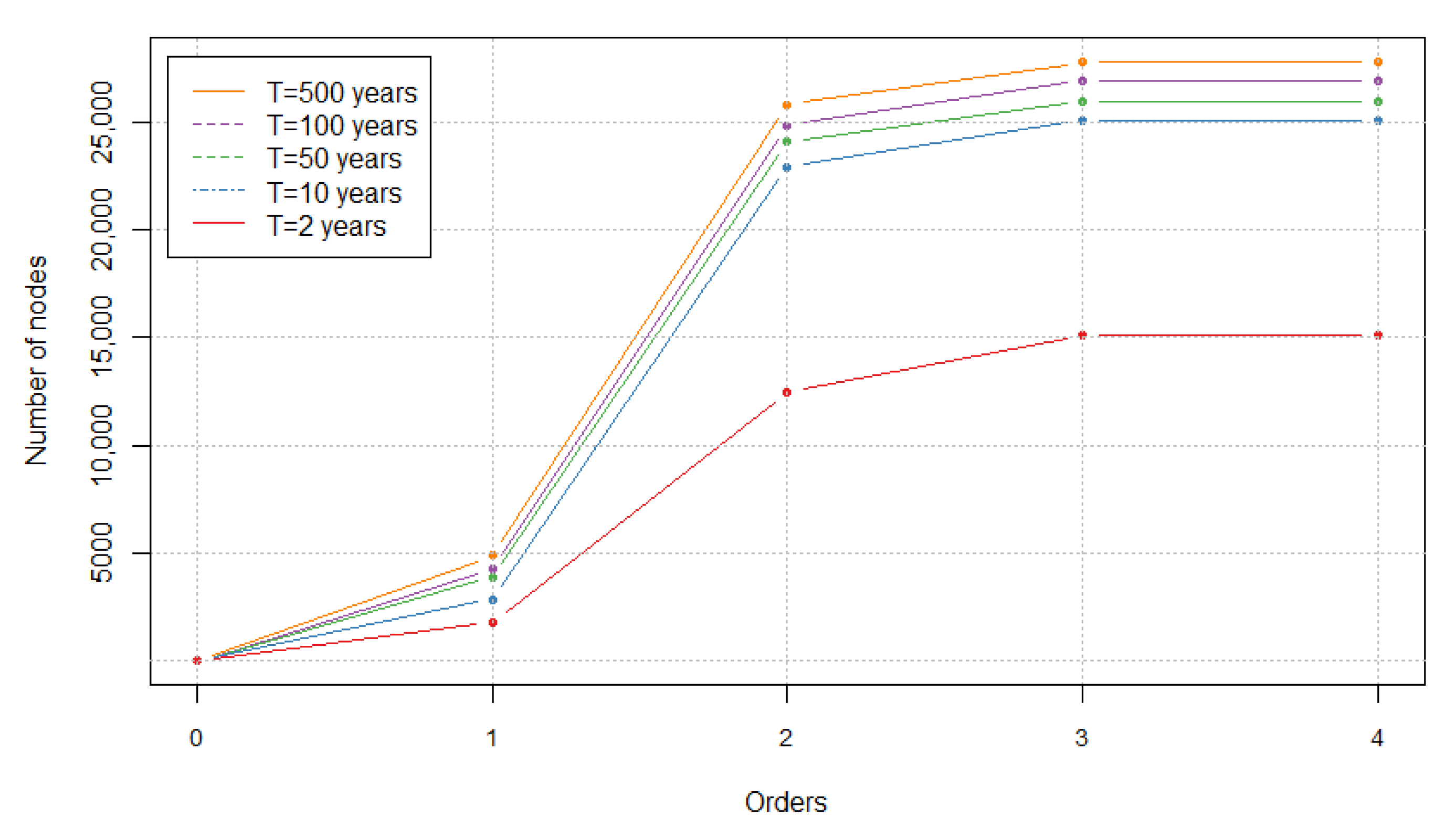
• to use the graph representation of a system as the basis for assessing higher-order impacts and cascading effects for different return periods (T), based on the propagation of impacts along graph links; and
• to illustrate how different impact mitigation measures can be formulated based on systemic information provided the analysis of graph properties, taking into account indirect impacts.

2. Methodology

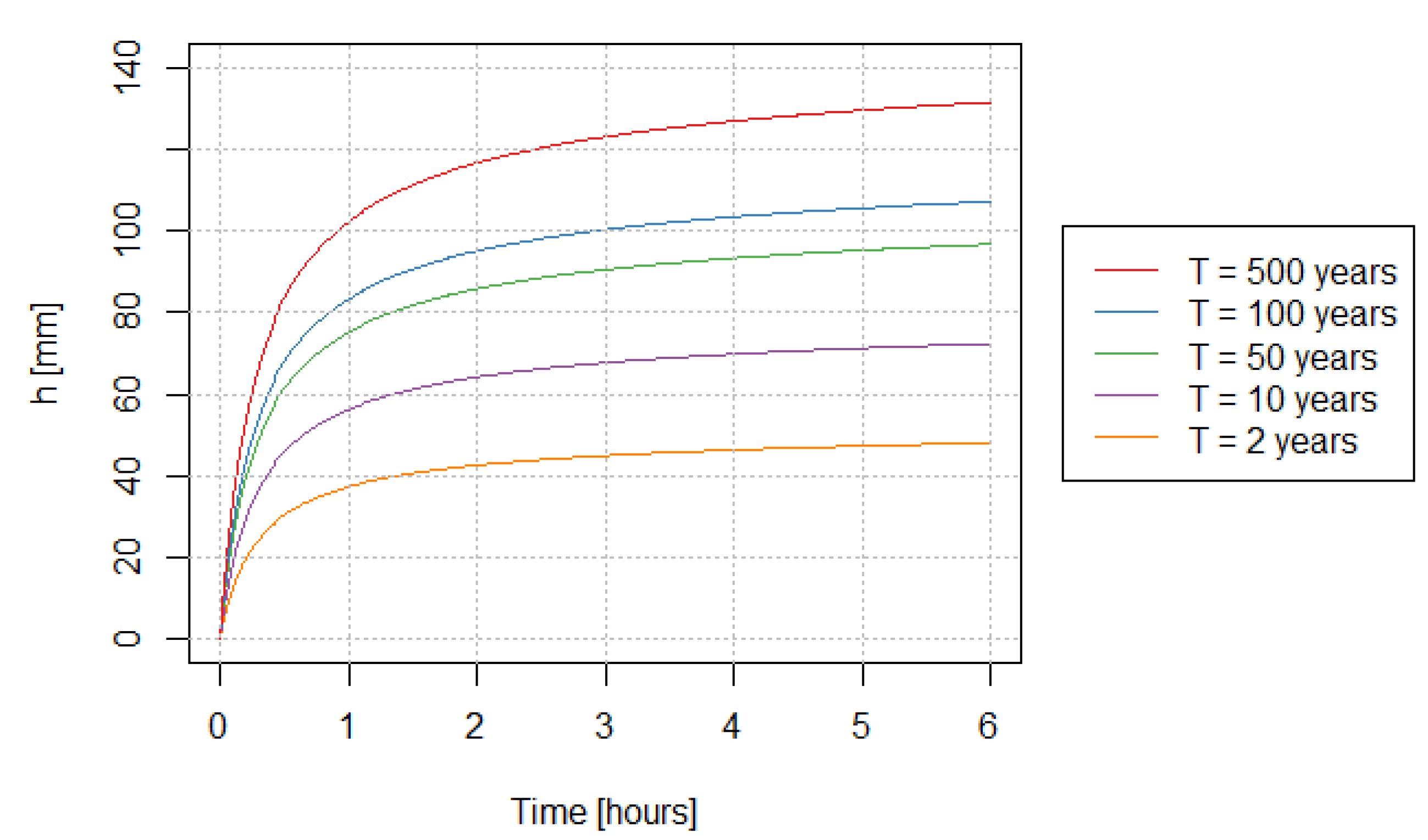
2.1. Hazard Modelling

Hazard identification and assessment are carried out by using the Storm Water Management Model developed by the United States Environmental Protection Agency (EPASWMM) [31], which has been adopted in many works in the scientific literature (e.g., [32,33,34,35]). This software can model the response of an urban catchment to rain events, while representing the external urban surfaces as planes featuring pre-assigned values of area, width, and slope. The runoff leaving the planes enters the underground system through the junctions present at channel ends and is then routed inside the channels up to the outlet(s) using De Saint Venant equations [36]. At each junction, the mass conservation equation is applied to balance entering and outgoing flows. In correspondence to intense rain events, backwater effects can take place, causing junctions to get surcharged. As a result, water goes out of the underground system, causing floods in the urban environment. The thorough assessment of flood extension and levels would require 2D flood propagation models to be used. However, if an urban territory is inside a basin, the propagation effects can be neglected, and flood extension and levels can be simply assessed by distributing flood volumes over territory, starting from the lowest ground elevations. This can be accomplished by using simple Geographic Information System (GIS) procedures [37].

In EPASWMM, the structure of the urban drainage networks needs to be defined in terms of channel paths, lengths, shapes, and sizes. Then, each junction, which can be a node in common between two adjacent channels, the starting node of a channel, or the final outlet of the system, can be connected to an external catchment. Catchments must be associated with a rain gauge, in which hyetographs can be implemented as time series to represent synthetic rain events of different return periods.

2.2. Graph Construction

This work demonstrates an approach to assess impacts beyond direct tangible damage, integrating the hazard analysis with a graph representation of a complex system. While the traditional reductionist risk assessment framework considers each exposed element individually, a graph representation is able to account for interactions between exposed elements at risk, which is key to a more comprehensive understanding of risk.

Graphs can be used to represent physical elements in the Euclidean space (e.g., electric power grids and highways) or entities defined in an intangible space (e.g., collaborations between individuals). Formally, a graph G consists of a finite set of elements V(G) called vertices (or nodes), and a set E(G) of pairs of elements of V(G) called edges (or links) [38]. The mathematical properties of a graph can be studied using graph theory [39,40]. Such properties, e.g., degree, hub and authority, are useful metrics for analysing the graph structure (i.e., network topology, and arrangement of a network) and in the present context may be used to characterize a collection of exposed elements from a systemic viewpoint (e.g., [41]).

The complete procedure to construct a graph representing a system of exposed assets is presented in Arosio et al. (2020) [29] and its two main steps are summarized here. First, the conceptual network is defined by means of two types of network objects, nodes (vertices) and links (edges), and by specifying their characteristics. Nodes can theoretically represent all the entities to be analysed: physical elements like single buildings, fire stations, and electric towers; supply of services such as those provided by schools, hospitals, and fire stations; or even beneficiaries such as population in general, or students, or elderly people more specifically. Links can be of different types according to the nature of the connection: physical, geographical, cyber, or logical [42]. Second, once the network has been conceptually defined, it is necessary to construct the actual connections between all elements. In fact, the conceptual network determines only the existence of connections between categories of elements, it does not define which specific node of one typology is linked to a specific node of another typology. Therefore, it is necessary to define rules that establish connections between single nodes. These connections can be represented either by a list of pairs of nodes or by an adjacency matrix.

2.3. Impact Assessment

Arosio et al. (2020) [29] propose analysing the properties of both the entire graph and single nodes. The global properties show how the whole system is vulnerable to an external perturbation, while the properties of single nodes underline which parts of the system are more critical for the entire system. The analysis of properties provides valuable information on the system. However, in order to assess risk and realize a proper DRR strategy, this information needs to be integrated and overlapped with hazard information (e.g., intensity, extension, and probability of occurrence). In the present work, the impact is computed by integrating the hazard for different return periods with the exposed network. The total impact considers both direct impact (D) and indirect impact (I).

For the direct impact, recent literature considers the overall amount of physical damage to assets (D) equal to the cost to repair and/or replace them, i.e., the sum of the cost to restore the damage (C_n) of all the nodes N that are hit by the hazard [43]. Under this condition, the direct physical impact is a function of the number of hit nodes (N), the hazard intensity (H_n) at each node n, and its physical vulnerability (V_n):

$$D={\displaystyle \sum }_{n=1}^N{C}_n\left(H_n,V_n\right)$$

(1)

The indirect impact (I) considers the overall amount of tangible losses generated by cascading effects due to the direct damage (D), i.e., the sum of the economic loss (L_S) of all the services S that are interrupted. In this specific definition, the indirect impact is a function of the number of services lost (S), the typologies of services (T_s), and economic values (V_s) associated to each typology value.

$$I={\displaystyle \sum }_{s=1}^S{L}_s\left(T_s,V_s\right)$$

(2)

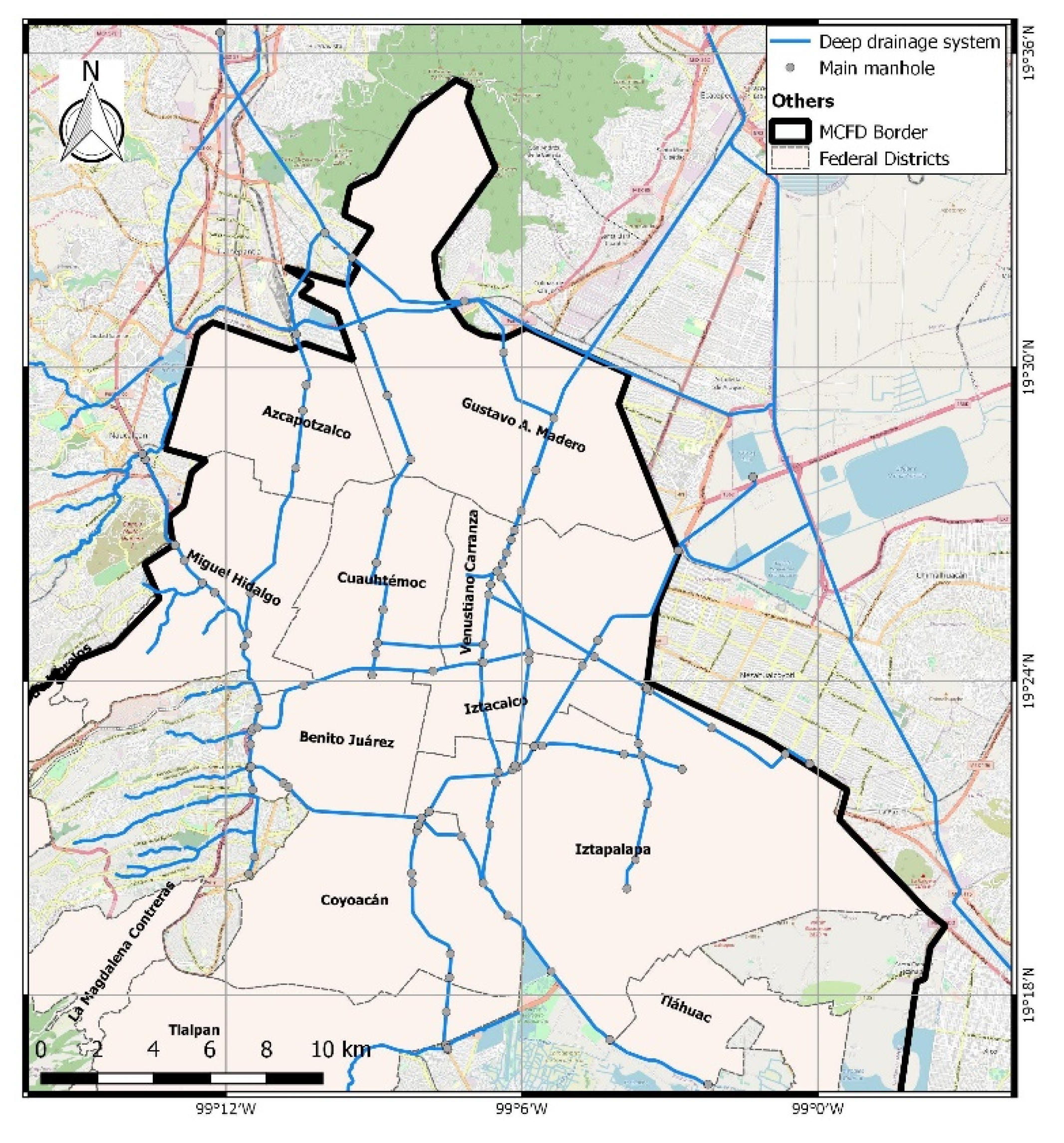
3. Application: Mexico City

Mexico City is one of the most hazard-prone cities in the world, due to the frequent occurrence of floods, landslides, subsidence, volcanism, and earthquakes. The Mexico City Metropolitan Area (MCMA), situated in a high mountain valley (approximately 2200 m a.s.l.), is one of the largest urban agglomerations in the world. Located in a closed basin of 9600 km², MCMA spreads over a surface of 4250 km². The MCMA has an estimated metropolitan population of about 21.2 million people, equal to 18% of the country’s population, and generates 35% of Mexico’s gross domestic product [44]. This application study focusses on Mexico City (also called the Federal District—MCFD), where approximately 8.8 million people live. The choice of MCFD as a pilot case allows showing the importance of interdependencies in assessing the total impact in a complex urban environment. Tellman et al. (2018) [45] show how the risk in Mexico City’s history has become interconnected and reinforced. In fact, as cities expand spatially and become more interconnected, risk becomes endogenous. Urbanization, driven by population growth, increases the demand for water and land in many parts of the world [46], which is well represented by the choice of Mexico City as case study. Furthermore, the impact estimated in the present work is expected to worsen in the future, due to the soil subsidence phenomenon in progress, which is expected to deteriorate the hydraulic capacity of the drainage system.

3.1. Description of the Application

3.1.1. Hazard Simulation

Rainfall patterns associated with different return periods were obtained through the uniform depth duration frequency curve (DDF) for the entire MCFD [47]. In particular, Chicago hyetographs with a duration of 6 h [48] and with peak located at 2.1 h were constructed starting from the DDF curve [49]. Figure 1 presents the DDF curves computed for different return periods, which were used in the analysis.

The EPASWMM model of the main urban drainage system, serving a total area of 1586 km², was constructed starting from data made available by the Engineering Institute of the National Autonomus University of (UNAM) México D.F. The model has 109 junctions (one for each catchment), and 98 underground channels with Strickler roughness set at 52 m^1/3/s, the typical value for masonry walls [48] and consider the condition of possible failure of the pumping system (see Figure 2 for the layout of the channels).

The model was used to simulate hydrology and hydraulics in Mexico City, i.e., runoff formation from external catchments and flow-routing in underground channels, respectively, as a result of the rainfall patterns described above. Water volumes going out from each surcharged node of the model were lain on its associated urban catchment, starting from the lowest areas close to the node itself. Incidentally, the neglection of flood propagation over the territory can be considered an acceptable assumption, due to the basin-shaped orography.

By applying the mass conservation equation to balance entering and outgoing flows at each junction, EPASWMM estimates the hydrograph of water that comes out when the piezometric curve exceeds the surface level. Furthermore, in a GIS environment, the volume-depth and depth-area functions for each basin were computed using a five-meter resolution digital terrain model (DTM). Knowing the volume from the outgoing hydrographs and using the functions mentioned above, the flood extension was evaluated independently for each basin at different return periods.

3.1.2. Network Conceptualization and Graph Construction

The six following critical typologies were selected to for this illustrative pilot study: fire stations, fuel stations, hospitals, schools, crossroads, and blocks [29]. These six typologies do not intend to cover all possible typologies of elements in the city, but rather to illustrate the methodology by representing different types of both tangible and intangible services. The simulation uses blocks instead of population, as this enables a reduction in computational demand by lowering the number of nodes from 8 million to a few tens of thousands. Furthermore, the analysis considers a limited number of central nodes of the city’s transportation network (i.e., crossroads) as providers of the transportation service to other elements. This approach does not aim to be representative of the complete behaviour of the road network system (e.g., [50]), but it does allow considering the transportation network in the analysis in a simplified manner. All the typologies, numbers of elements and the connections between them are presented in

Table 1. List of nodes adopted in the network conceptualization [29].

Network Conceptualization	Type of Nodes	Number of Elements	Service Provided	Destination of the Service
		17	Transportation	Fire Stations, Schools, Hospitals, Fuel Stations, and Blocks
		11	Recovery	Schools, Hospitals, Fuel Stations, and Blocks
		103	Power	Blocks
		39	Healthcare	Blocks
		130	Education	Blocks
		64,282	-	-

. The data utilized to build the network were provided by the Engineer Institute UNAM México D.F.

The mathematical graph, built from the list of nodes and links considered, was obtained using the open source igraph package for network analysis of R environment (http://igraph.org/r/), while the full library of functions adopted are made available by Nepusz and Csard (2018) [51].

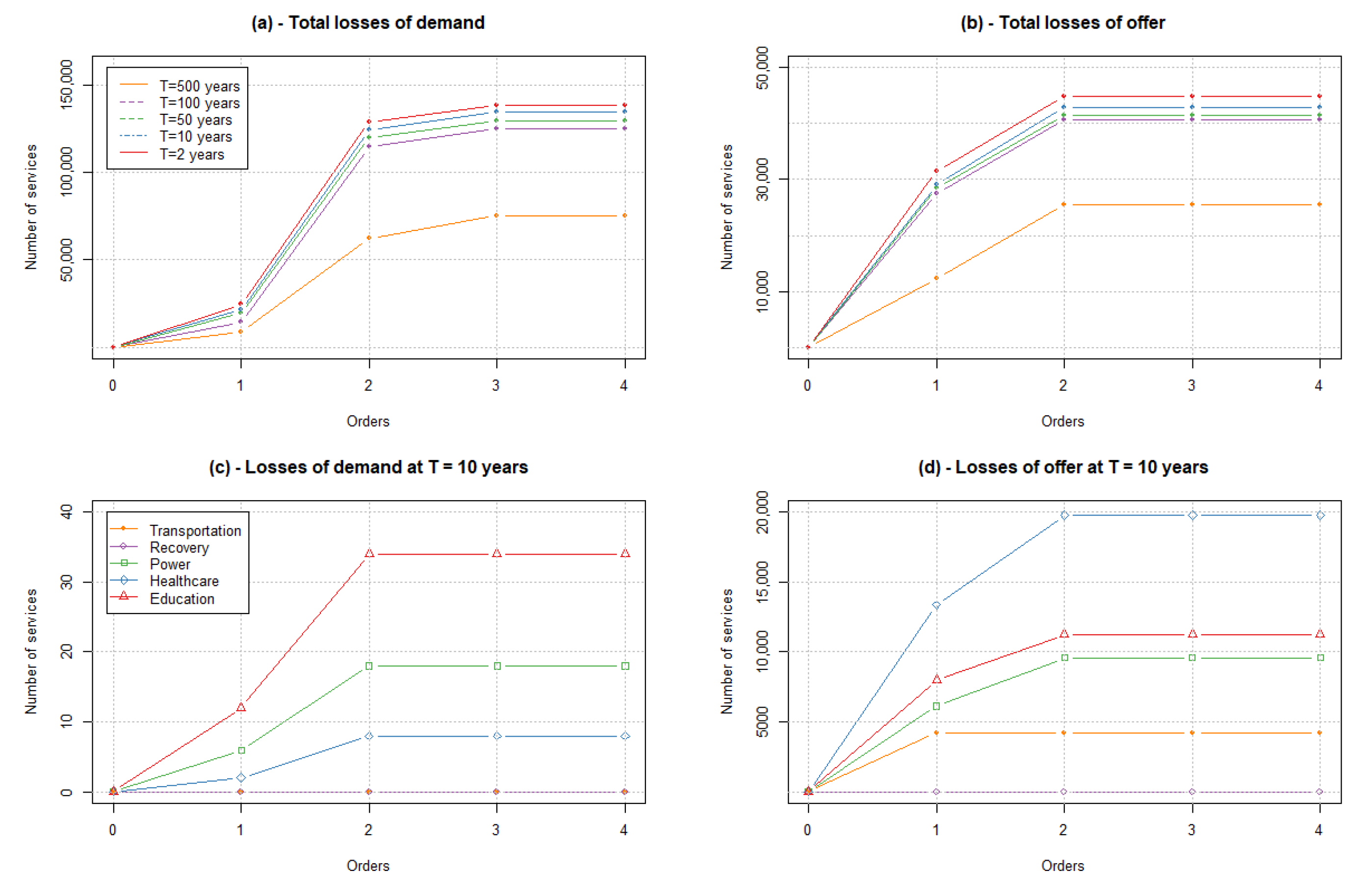
3.1.3. Impact Analysis

For the estimation of the direct impact of the nodes, simplified binary vulnerability functions were adopted, consisting of zero damage for the nodes outside of the flooded area, and full damage and loss of functionality for the nodes inside the flooded area. This means that directly impacted nodes are assumed to lose their capacity to provide services, and also their demand for such services. Admittedly, this simple assumption does not realistically represent the estimation of direct damage. However, it is considered acceptable in light of the main focus of this work, which is to investigate and demonstrate the potential of a graph in representing and exploring indirect impacts.

The analysis of the indirect impact refers number of services, as opposed to number of nodes in the direct impact analysis. In fact, indirect impacts are represented here by the difference between the number of the services, i.e., links, existing before the hazardous event and the number of services at the final state, after the cascading effects $\left(S_{initial}-S_{final}\right)$. This analysis could be enhanced with estimates of economic losses corresponding to disrupted services (e.g., related to the fuel sector [52] or the education sector [53]) and/or with economic models to estimate overall economic impacts at a regional scale (e.g., [26]), although these are not carried out here as they are outside the scope of the present article.

The nodes directly impacted by the flood generate a cascading effect into the graph, whereby the propagation of the impact follows the nodes that have lost at least one service from their providers. This propagation process is modelled by creating a new graph (G₁) where nodes directly affected by the hazard (i.e., flooded nodes) are removed from the original graph (G₀). After that, the degree-in, representative of the number of received services, of each node in G₁ is compared with the corresponding degree-in in G₀. By deleting all nodes experiencing a degree-in reduction from G₀ to G₁, graph G₂ is obtained. This process is iterated until there are only unaffected nodes in the graph to produce the final graph G_final, which corresponds, to the final state of the affected system.

In this application, two different indirect impacts (i.e., here measured in term of services lost) are investigated: loss of service providers (S_P, i.e., suppliers) and loss of service receivers (S_R i.e., consumers). In fact, after a hazardous event, nodes that provide services can experience a loss of demand (L_D) from their receivers (R) that are affected by the event. Conversely, the receivers can observe a loss of services (L_S) from their providers (P) after the hazardous event. The loss of provider services (S_P) and of receiver services (S_R) can be computed as

$$S_P={\displaystyle \sum }_{i=1}^M{\displaystyle \sum }_{j=1}^N{\omega }_{i,j}$$

(3)

and

$$S_R={\displaystyle \sum }_{i=1}^M{\displaystyle \sum }_{j=1}^N{\phi }_{i,j},$$

(4)

where $\phi$ and $\omega$ are respectively the degree-in and degree-out of the jth node that at the ith order has been deleted; N is the number of deleted nodes at step i and M is the last order of loss propagation (i.e., 4 orders in this application). The loss of demand is computed by summing the degree-in of the deleted nodes, while the loss of services is computed by summing the degree-out of the deleted nodes.

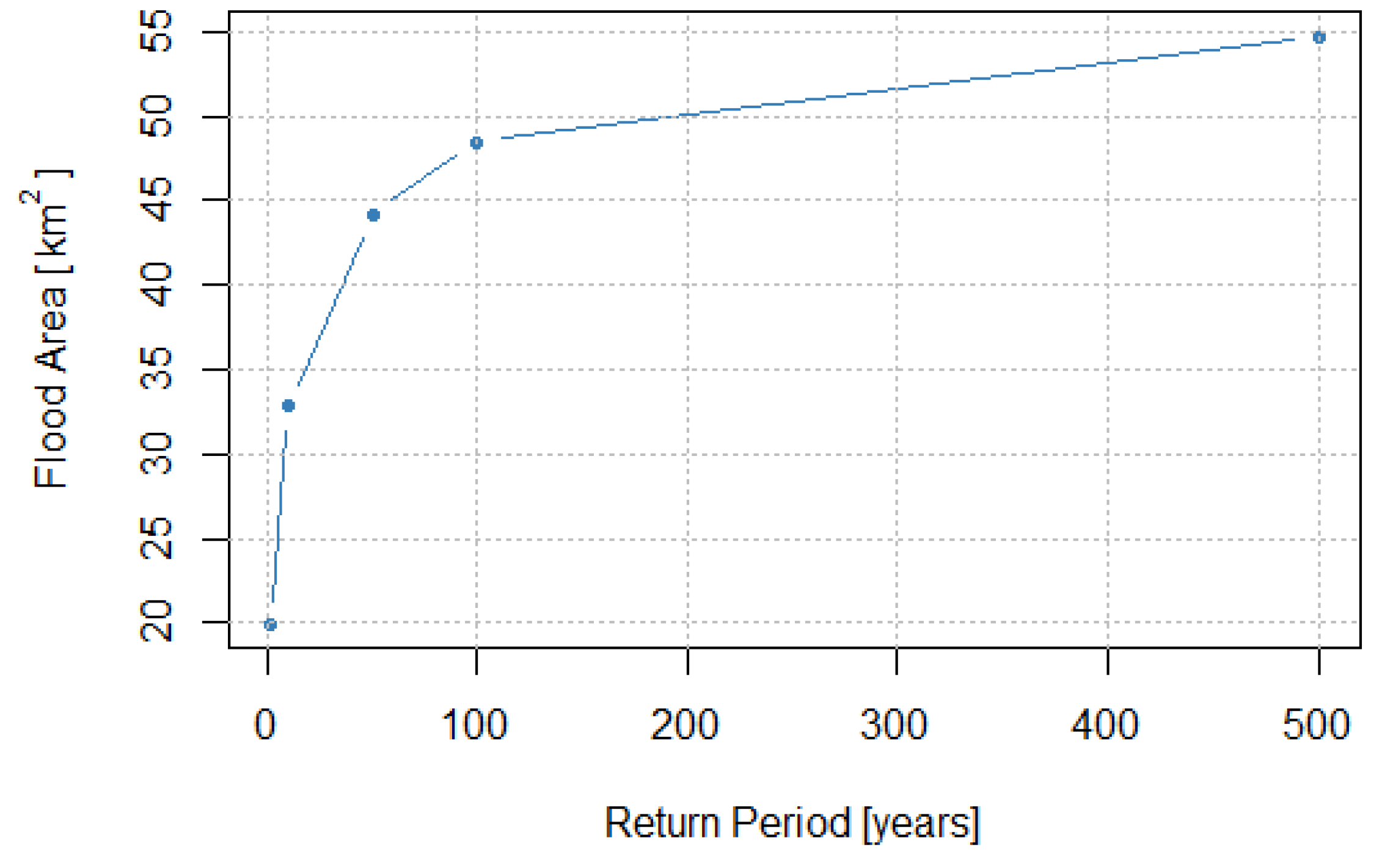
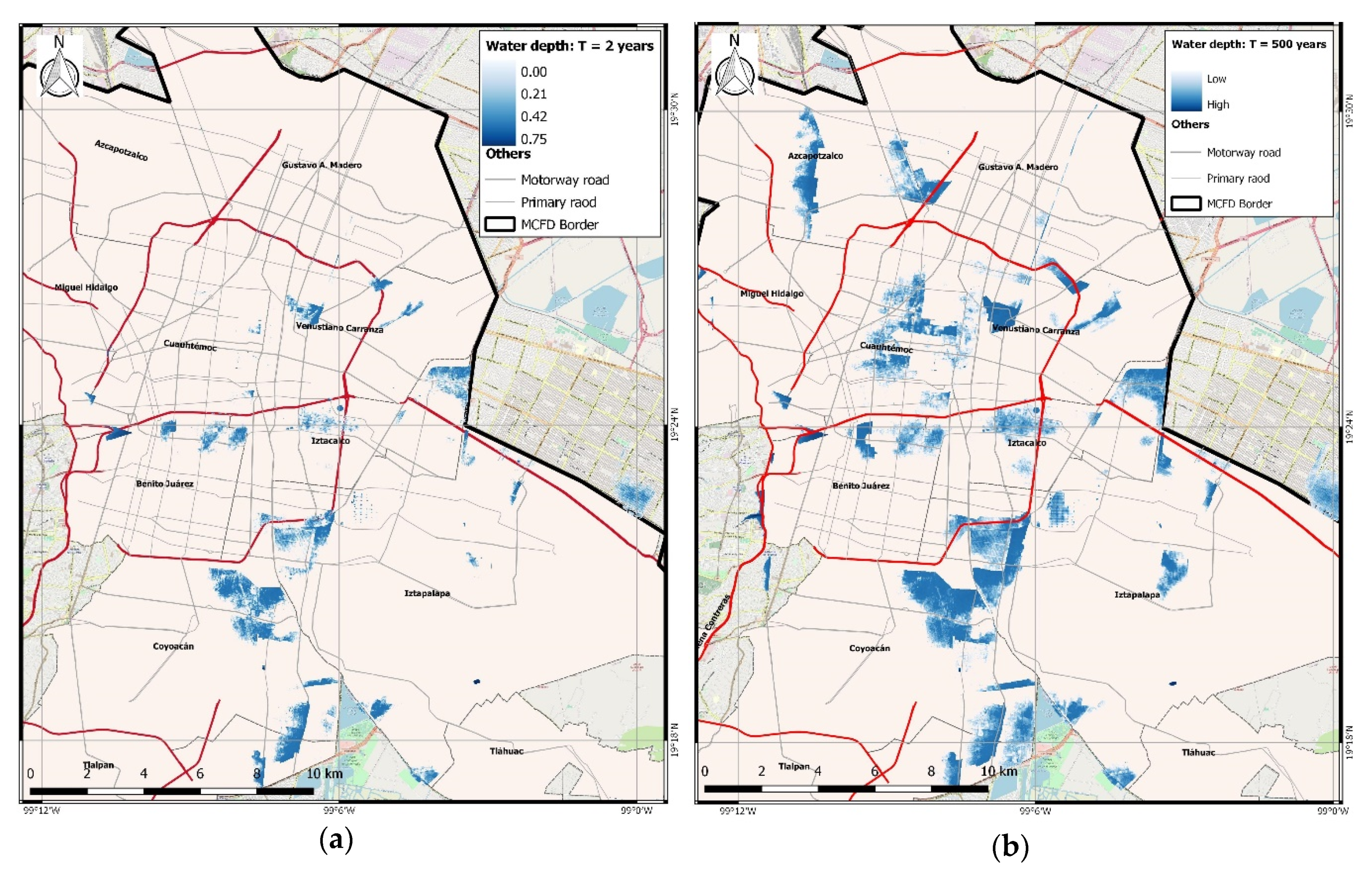
3.2. Flood Hazard and Impact Results

This section shows the results obtained from the hydrological and hydraulic simulations, followed by the estimation of direct and indirect impacts. The impacts are previously presented in terms of cascading evolution of affected nodes and later in term of lost connections. It is also presented for each typology of service whether the impact is due to the loss of service provider or of receiver demand and illustrates how different flood mitigation measures can be formulated based on systemic information provided the analysis of graph properties.

The hazard analysis provided the pluvial flood areas associated with the precipitation at each specific return period. As expected, Figure 3 shows that the total flood area increases with growing return period: from 20 km² at the 2-year return period up to 55 km² at the 500-year return period.

For illustration, Figure 4 presents the areas associated with a flood with the 2- and 500-year return periods, respectively the minimum and maximum considered in this study. In both cases, most water depth values are within realistic ranges (e.g., up to 1.20 m for the 500-year return period flood), with only a limited number of outliers located mostly at the borders of the considered basins. While a more comprehensive flood hazard assessment would be possible by using 2D flood propagation models, these results are considered suitable for the specific scope of this work, which focuses on demonstrating a graph-based approach for higher-order impact assessment and risk mitigation.

Traditional approaches estimate the direct impacts considering only the exposed elements hit by the flood. Instead, the proposed approach can simulate the evolution of cascading effects after some elements are directly hit. Figure 5 shows the evolution of cascading effects of affected nodes at different orders. At each order, the graph was obtained by removing the nodes that were affected in the previous order. Order 0 is the original graph, order 1 is reduced by the nodes that were affected directly by the flood, and from orders 2 to 4 the graphs were obtained by removing indirectly affected nodes, as explained previously. The number of nodes impacted by the event increases when moving from order 1, which represents the directly affected nodes, to order 3, which is associated with the maximum number of nodes affected by the event. The cascading effects stop at order 3 because there are no new nodes affected by parent nodes after that point. Figure 5 shows less than 5000 nodes directly affected for each return period, specifically 3% of the nodes (1818 nodes) and 8% of the nodes (4904 nodes) are flooded for the return periods of 2 years and 500 years, respectively. Instead, the total number of nodes affected at the end of the cascading effects ranges from 23% to 43% of the entire graph, at the 2- and 500-year return periods, respectively.

Comparing the shape of the curves in Figure 5, a particular behaviour is remarked between the 2- and 10-year return periods when moving from order 1 to 2. In fact, the difference in number of affected nodes between the two return periods is much higher at order 2. The increment of nodes affected at each order, after the direct impact (above order 1), is not proportional with the increment of flooded extension associated with different return period. This is a peculiar aspect of complex systems, in which large-scale secondary events play a not-negligible role.

An explanation for this can be found in Figure 6, which shows the propagation of the effects not only inside the flooded areas, but also outside and potentially over the entire network. Figure 6 shows in red the nodes that are directly impacted (i.e., inside the flood area), in orange the nodes that are indirectly impacted due to the absence of service from the provider nodes inside the flood area (black stars at order 1), and in yellow the nodes at order 3 that are indirectly impacted due to the absence of service from the provider nodes affected at order 2 (grey stars). Since at order 3 there are no new affected providers, the propagation effects stop and the number of impacted nodes at order 4 do not increase. In comparison with the 2-year return period, there is a larger number of nodes affected at order 2 in the 10-year-return period. This happens because the flood directly impacts a hospital, which is not reached by the flood at the 2-year return period. This hospital is an important central node of the graph, which has the capability of influencing many other nodes due to its role of hub. In fact, this node provides the healthcare service to many other nodes, and as shown by the hub analysis carried out in Arosio et al. (2020) [29], it has the highest hub value of the entire system. Figure 6 shows, for the larger return period, more numerous orange nodes (i.e., nodes indirectly impacted at order 2) in the south-east part of the city. This large area, characterized by blocks with higher authority values [29], gets affected due to the absence of service provided by the hospital mentioned above. According to these results, the blocks with higher authority are the ones that depend on the services from the providers with higher values of hubs. For this reason, the floods that hit such hubs undermine a considerable part of the network as is evident for floods with T above 2 years. The strong correlation between hubs and authority explains these results. However, it is necessary to underline that these outputs also reflect the assumption of the rules of proximity adopted in this model, where the network has no redundancy by construction [29]. The redundancy can change the values of hub and authority of the nodes and can therefore influence the magnitude of cascading impacts that are presented in the next section.

Beyond the evolution of the cascading effects, the comparison between the direct and total impact associated with the flooded areas at different return periods has been investigated and is presented in Figure 7. This figure confirms that while the number of directly impacted nodes is proportional to the flooded area, this is not the case for the total number of impacted nodes, which also considers the indirect impact. As emphasised before, the non-proportional increment is more evident when moving beyond the 10-year return period flood, past which the node with the highest hub value is flooded.

The proposed methodology offers the possibility to investigate not only the nodes but also the connections that are affected during the evolution of the event. This innovative perspective is presented in Figure 8, which shows the probability of observing the loss of services for both direct and indirect impact. In both cases, the curves present the typical shape of risk exceedance probability curves. This figure highlights the much larger numbers of lost services for the indirect impact relative to the direct one, especially for rarer events, where direct impact is only a minor part of the total impact.

A more exhaustive explanation of the service lost is provided by the analysis of the causes that generate the lack of services. Figure 9 shows the extent to which the lost services ($\Delta S$) is due to the absence of receivers’ demand (L_D on the left) and the absence of offer from providers (L_O on the right). The high values of total demand loss at each return period are mainly driven by the impact on the population; in particular, for the return period of 2 years, the total loss of demand is below 80,000 in comparison with the highest return period featuring a loss of demand above 120,000. The total losses of offers are due to the impacts on the providers and the values are about one third of the total loss of demands. The plot for 10-year return period highlights that the loss of services is mainly due to the absence of service provided by the hospital, which is confirmed by the hub analysis mentioned previously [29]. Conversely, education is the sector across providers that generates more losses, followed by power and healthcare, whereas crossroads and fire stations do not cause loss of demand.

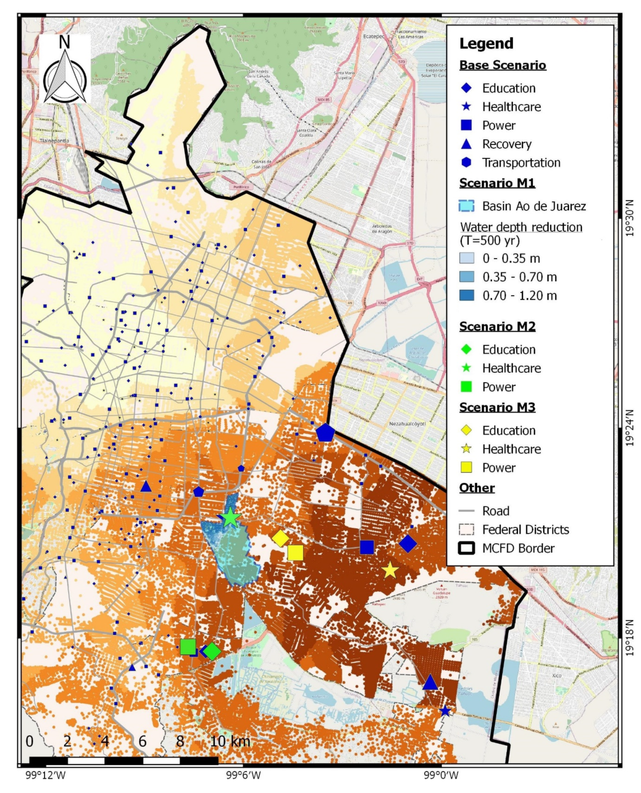
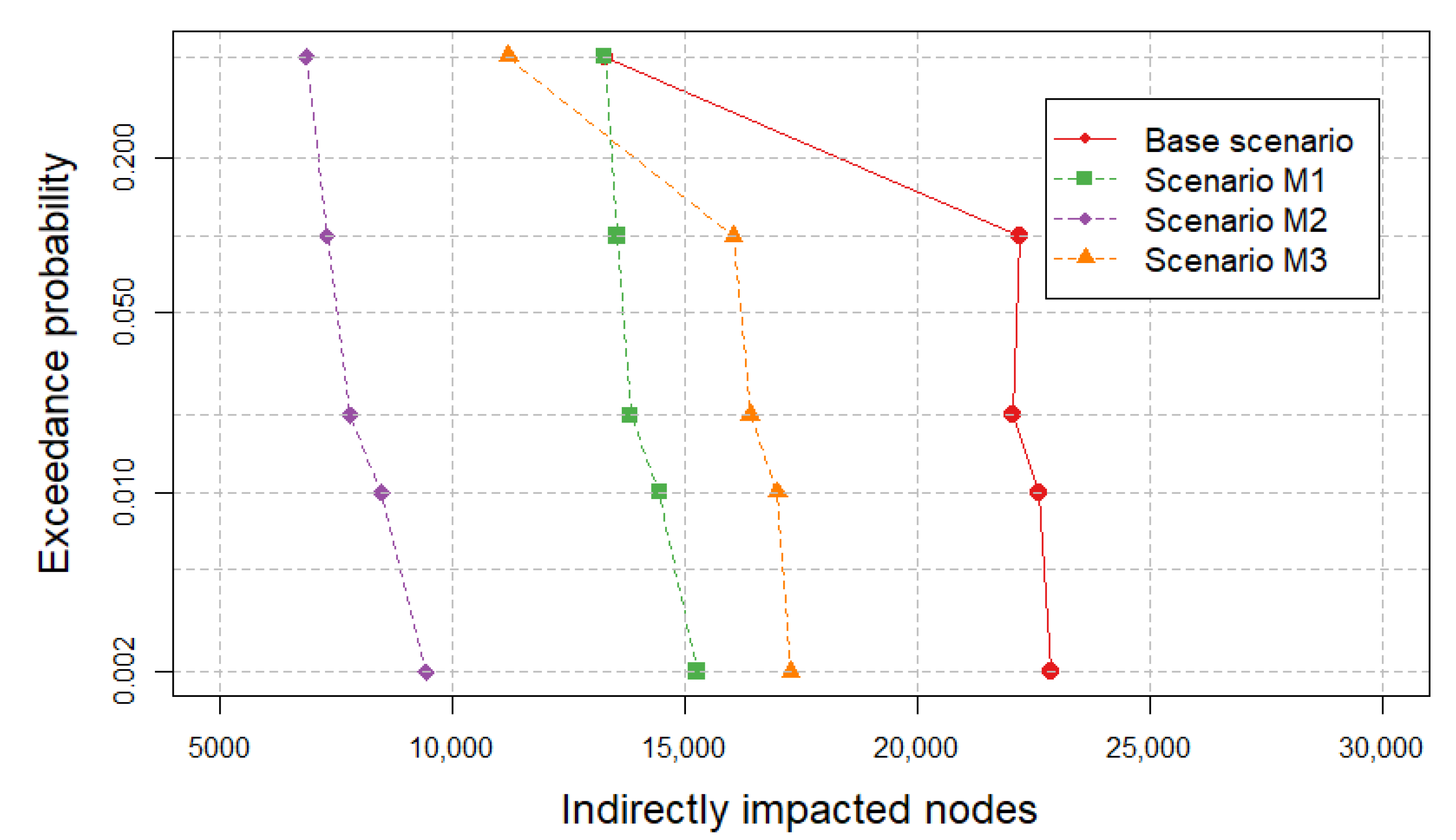
3.3. Mitigation Scenarios

The previous analysis highlights that indirect impacts must not be overlooked when assessing risk. Accordingly, such impacts should be taken into account for the implementation of effective risk mitigation measures, which traditionally tend to be based on the analysis of direct impacts only. The approach used here is able to characterize the system through various graph measures, which can then be used as a starting point for the identification of efficient solutions to mitigate risk, arising not only from direct impacts but also from higher-order effects. To illustrate this, three possible mitigation scenarios (M1, M2, and M3) are proposed. The definition of these hypothetical scenarios was based on information provided by certain graph properties, in particular, hub and authority values, as described next.

Scenario M1—Hazard mitigation: One of the most traditional approaches for mitigating flood risk is to implement measures that reduce the hazard intensity. Therefore, for scenario M1, we consider a hypothetical intervention in the Au De Uarez basin to increase its permeability and thus to reduce the volume of flooding from the drainage system in this specific basin. In the Au De Uarez basin, highlighted in blue in Figure 10, the hospital with the highest value of hub is located. We have considered an intervention that can reduce the waterproof area by up to 60%. As a result, by using equation

$$\mathsf{\Psi }={\mathsf{\Psi }}_P\left(1-A_{imp}\right)+{\mathsf{\Psi }}_{imp}\times A_{imp}$$

(5)

where $\mathsf{\Psi }$ is the weighted flow coefficient, ${\mathsf{\Psi }}_P$ and ${\mathsf{\Psi }}_{imp}$ are the flow coefficients respectively for permeable and impermeable area ($A_{imp}$) [54], the reduced flooded volume was calculated. Given the mitigated volume, using the volume–height curve characteristic of the basin, the post-intervention flood heights and extents were obtained. In this new configuration, the hospital is not flooded for any return period.

Scenario M2—Mitigation of the physical vulnerability: Another option to reduce risk is to intervene on the physical vulnerability of the exposed elements. In this alternative, we have chosen three elements that are within the flooded area and have the highest hub values as provided by the graph analysis: a hospital, a school, and a petrol station (highlighted in green in Figure 10). Considering the binary vulnerability functions adopted in this work, reducing the vulnerability means making the three elements waterproof without the loss of functionality. Note that this assumption does not intend to realistically represent the reduction in vulnerability provided by actual waterproofing measures (e.g., [55,56,57]), but rather to illustrate methodology for this specific scenario.

Scenario M3—Mitigation of the systemic vulnerability: The last scenario is aimed at mitigating the systemic vulnerability associated with the dependency of a large number of nodes on the three service providers identified in the previous scenario (i.e., the nods with the highest hub values). To achieve this, three new providers were added to the network: one hospital, one school, and one petrol station, highlighted in yellow in Figure 10. The choice of location was made considering the area outside the flood extents where nodes present the highest authority values [29].

Figure 11 shows the annual exceedance probability curved (i.e., risk curves), expressed in terms of number of indirectly impacted nodes, for the baseline and the three mitigation scenarios. Regarding scenario M1, the considered mitigation measure is effective for floods with return periods of 10 years and higher because the only benefitted provider is not affected by the 2-year return period flood (i.e., the hospital with hub value equal to 1). Scenario M2 returns the greatest reduction for any return period, which is reasonable given that waterproofing measures were considered for the three elements with the highest hub values. However, in practice, a complete mitigation of physical vulnerability is not attainable, and thus it is likely that flood above a certain return period would affect these elements to some extent. Scenario M3 also leads to an impact reduction for all return periods, although it is not as effective as M2 as implemented in this illustrative analysis. Nevertheless, risk is mitigated to some extent through a redistribution of services provided.

In order analyse the effectiveness of each mitigation scenario, we adopt the most widely-used metric to express risk, which corresponds to the integral of the annual exceedance probability curves shown in Figure 11. This approach may be employed even when losses are not expressed in economic terms [58], as is the case in this study, where our analysis is based on the number of indirectly affected nodes as a proxy for indirect impacts, for the purpose of illustration. For each scenario, we first compute a risk index R as the trapezoidal approximation of the area under the risk curve given by

$$R={\displaystyle \sum }_{i=1}^{H-1}\left(P_{i+1}-P_i\right)\frac{N_{i+1}-N_i}{2}$$

(6)

where H is the number of adopted hazard scenarios, P_i is the annual probability of occurrence of the ith hazard scenario (which is assumed to be equal to the inverse of its return period), and N_i corresponds to the number of impacted nodes. We then compute the effectiveness of the different mitigation actions as the reduction of the risk index in relative terms, given by

$$RM[\%]=\frac{R_B-R_j}{R_B}\ast 100$$

(7)

where R_B is the risk index for the baseline scenario and R_j is the risk index for the jth mitigation scenario.

Table 2. Impact mitigation of the indirect consequences for each scenario.

Scenario	RM [%]
M2 + M1	77.93
M2 + M3	74.74
M2	53.75
M1 + M3	45.16
M1	24.18
M3	20.99

shows the results for each mitigation scenario considered both individually and in combination, confirming the previously discussed results of Figure 11. In fact, it shows that M2, and any combination that includes it, are the most effective solutions at mitigating the indirect impacts.

4. Concluding Remarks

This work focussed on the analysis of the direct and indirect impacts of flood in a complex urban environment that is Mexico City. To this end, we first presented and applied methods for flood hazard assessment at different return periods, due to the spillage of rainwater discharges from surcharged underground drainage channels, under the assumption of pumping systems being out of service. Second, we proposed and applied a graph-based methodology to estimate the total impact of the reconstructed floods and illustrated how graph properties may be used to support the design of mitigation measures.

The results of the work pointed out that, consistently with engineering judgement, flood extensions and levels increase as the return period used for modelling the rainfall grows. Naturally, these are accompanied by the increase of the number of nodes directly affected by the flood. The use of a graph representation of the system then enables the assessment of indirect impacts associated with the flood. The results pointed out that, differently from the direct damage, indirect impacts—and consequently, total impacts—are the result of the number of nodes incrementally affected at each order, which are not proportional to the growth of the flooded area associated with different return periods. This behaviour can be ascribed in this case study to the flooding of an important hub of the graph; thus, generating large cascading effects. Similar situations are expected to occur in other comparable urban environments.

Furthermore, the study showed how the network experiences loss of services at providers (S_P) and receivers (S_R) for each specific typology of nodes at different orders and return periods. The total losses of service are due to the impacts on the providers and the values are about one third of the total loss of demands, which are mainly driven by the impact on the population. The highest loss of offer is mainly due to the interruption of services provided by the healthcare sector. Conversely, education is the sector that has the highest loss of demand. The impact curves of the lost services in the network showed the extent to which the total impact is larger than the direct impact. In fact, the results of this work confirmed that, especially for extreme rain events, considering only the direct impact leads to a significant underestimation of the total consequences. Furthermore, the last part of the work proved the graph representation of the impacts to be a useful tool for driving decision makers in the choice of the interventions to carry out in the territory, which can include the mitigation of hazard and of physical and systemic vulnerability.

Due to the complexity of the case study and to the unavailability of some data, simplifying assumptions were made along the way, as far as the assessment of hazard, vulnerability, and exposure. In terms of the hazard component, flood extension and levels were assessed by distributing flood volumes over the territory, while neglecting the 2D propagation. Regarding the vulnerability, flood impact was assumed to reduce the services supplied by the directly and indirectly affected nodes immediately to zero through a binary vulnerability function, whereas common sense suggests the loss of functionality to be a growing function of the hazard intensity. Finally, for the exposure component, the risk mitigation measurements adopted are based on the number of nodes and services impacted and not on economic values of the assets and services.

The dynamic evolution from direct to indirect impacts is analysed in this paper by the transformation of the graph at different orders. A more comprehensive analysis should consider the time evolution of the phenomena and not only a progressive order of states. The introduction of the time-element would also allow considering the economic consequences of service interruptions. As an example, regarding the education sector, Sadique et al. [59] investigate the costs of work absenteeism, in terms of paid productivity loss, of care givers who must stay at home during periods of school closure; analogous economic considerations can be done for other sectors. This is outside the scope of the present study, which in this context provides a framework on top of which further economic analyses may be carried out. Future work will be dedicated to incorporating such analyses within the proposed framework, in order to obtain more accurate estimates of the overall impacts of floods in interconnected urban systems.

References

1. Adikari, Y.; Yoshitani, J. Global Trends in Water-Related Disasters: An Insight for Policymakers—The United Nations World Water Assessment Programme; The United Nations Educational, Scientific and Cultural Organization: Paris, France, 2009. [Google Scholar]
2. Jiménez Cisneros, B.E.; Oki, T.; Arnell, N.W.; Benito, G.; Cogley, J.G.; Döll, P.; Jiang, T.; Mwakalila, S.S.; Kundzewicz, Z.; Nishijima, A. Freshwater resources. Clim. Chang. 2014 Impacts Adapt. Vulnerability Part A Glob. Sect. Asp. 2015, 229–270. Available online: https://scholarbank.nus.edu.sg/handle/10635/133175 (accessed on 16 June 2020).
3. Cramer, W.; Yohe, G.W.; Auffhammer, M.; Huggel, C.; Molau, U.; Da Silva Dias, M.A.F.; Solow, A.; Stone, D.A.; Tibig, L.; Leemans, R.; et al. Detection and attribution of observed impacts. Clim. Chang. 2014 Impacts Adapt. Vulnerability Part A Glob. Sect. Asp. 2015, 979–1038. Available online: https://www.zora.uzh.ch/id/eprint/105700/1/2014_HuggelC_WGIIAR5-Chap18_FINAL%20.pdf (accessed on 16 June 2020).
4. Arnell, N.W.; Gosling, S.N. The impacts of climate change on river flood risk at the global scale. Clim. Chang. 2016, 134, 387–401. [Google Scholar] [CrossRef] [Green Version]
5. Kreibich, H.; Müller, M.; Thieken, A.H.; Merz, B. Flood precaution of companies and their ability to cope with the flood in August 2002 in Saxony, Germany. Water Resour. Res. 2007, 43, 1–15. [Google Scholar] [CrossRef] [Green Version]
6. Zhou, Q.; Mikkelsen, P.S.; Halsnæs, K.; Arnbjerg-nielsen, K. Framework for economic pluvial flood risk assessment considering climate change effects and adaptation benefits. J. Hydrol. 2012, 414–415, 539–549. [Google Scholar] [CrossRef]
7. Muis, S.; Güneralp, B.; Jongman, B.; Aerts, J.C.J.H.; Ward, P.J. Science of the Total Environment Flood risk and adaptation strategies under climate change and urban expansion: A probabilistic analysis using global data. Sci. Total Environ. 2015, 538, 445–457. [Google Scholar] [CrossRef]
8. Grossi, P.; Kunreuther, H. Catastrophe Modeling: A New Approach to Managing Risk; Catastrophe Modeling; Kluwer Academic Publishers: Boston, MA, USA, 2005; Volume 25, ISBN 0-387-23082-3. [Google Scholar]
9. Balbi, S.; Giupponi, C.; Gain, A.; Mojtahed, V.; Gallina, V.; Torresan, S.; Marcomini, A. The KULTURisk Framework (KR-FWK): A conceptual framework for comprehensive assessment of risk prevention measures—Project deliverable 1.6. SSRN Electron. J. 2010. [Google Scholar] [CrossRef]
10. DEFRA (Department for Environment Food and Rural Affairs Flood Management Division). Surface Water Management Plan Technical Guidance; DEFRA: London, UK, 2010.
11. Parker, D.J.; Priest, S.J.; Mccarthy, S.S. Surface water flood warnings requirements and potential in England and Wales. Appl. Geogr. 2011, 31, 891–900. [Google Scholar] [CrossRef]
12. SEPA. Planning Guidance Strategic Flood Risk Assessment: SEPA Technical Guidance to Support Development Planning; SEPA: Stirling, Scotland, 2015; pp. 1–21. [Google Scholar]
13. Pitt, M. The Pitt Review: Learning Lessons from the 2007 Floods; Cabinet Office: London, UK, 2008.
14. Ochoa-Rodríguez, S. Urban Pluvial FLood Modelling: Current Theory and Practive. Available online: https://www.raingain.eu/sites/default/files/wp3_review_document_0.pdf (accessed on 16 June 2020).
15. James, W.; Rossman, L.A.; James, W.R.C. User’s Guide to SWMM5, 13th ed.; CHI: Guelph, ON, Canada, 2010; ISBN 9780980885330. [Google Scholar]
16. CH2M Flood Modeller Suite. Available online: https://www.floodmodeller.com/ (accessed on 16 June 2020).
17. DHI Mike 2020. Available online: https://www.mikepoweredbydhi.com/mike-2020 (accessed on 16 June 2020).
18. Aronica, G.T.; Candela, A.; Fabio, P.; Santoro, M. Estimation of flood inundation probabilities using global hazard indexes based on hydrodynamic variables. Phys. Chem. Earth 2012, 42–44, 119–129. [Google Scholar] [CrossRef]
19. Löwe, R.; Urich, C.; Sto, N.; Mark, O.; Deletic, A.; Arnbjerg-nielsen, K. Assessment of urban pluvial flood risk and efficiency of adaptation options through simulations—A new generation of urban planning tools. J. Hydrol. 2017, 550, 355–367. [Google Scholar] [CrossRef] [Green Version]
20. Russo, B.; Sunyer, D.; Velasco, M.; Djordjevic’, S. Analysis of extreme fl ooding events through a calibrated 1D/2D coupled model: The case of Barcelona (Spain). J. Hydroinform. 2015, 17, 473–491. [Google Scholar] [CrossRef]
21. Galuppini, G.; Quintilliani, C.; Arosio, M.; Barbero, G.; Ghilardi, P.; Manenti, S.; Petaccia, G.; Todeschini, S.; Ciaponi, C.; Martina, M.L.V.; et al. A unified framework for the assessment of multiple source urban flash flood hazard: The case study of Monza, Italy. Urban Water J. 2020, 17, 35–77. [Google Scholar] [CrossRef]
22. Penning-rowsell, E.; Johnson, C.; Tunstall, S.; Morris, J.; Chatterton, J.; Green, C.; Koussela, K.; Fernandez-bilbao, A. The Benefits of Flood and Coastal Risk Management: A Handbook of Assessment Techniques; Middlesex University Press: London, UK, 2005; ISBN 1 904750 51 6. [Google Scholar]
23. Merz, B.; Kreibich, H.; Schwarze, R.; Thieken, A. Assessment of economic flood damage. Nat. Hazards Earth Syst. Sci. 2010, 10, 1697–1724. [Google Scholar] [CrossRef]
24. Arrighi, C.; Brugioni, M.; Castelli, F.; Franceschini, S.; Mazzanti, B. Urban micro-scale flood risk estimation with parsimonious hydraulic modelling and census data. Nat. Hazards Earth Syst. Sci. 2013, 13, 1375–1391. [Google Scholar] [CrossRef] [Green Version]
25. Lüdtke, S.; Schröter, K.; Steinhausen, M.; Weise, L.; Figueiredo, R.; Kreibich, H. A Consistent Approach for Probabilistic Residential Flood Loss Modeling in Europe. Water Resour. Res. 2019, 55, 10616–10635. [Google Scholar] [CrossRef] [Green Version]
26. Sieg, T.; Schinko, T.; Vogel, K.; Mechler, R.; Merz, B.; Kreibich, H. Integrated assessment of short-term direct and indirect economic flood impacts including uncertainty quantification. PLoS ONE 2019, 14. [Google Scholar] [CrossRef] [Green Version]
27. Okuyama, Y. Economic modeling for disaster impact analysis: Past, present, and future. Econ. Syst. Res. 2007, 19, 115–124. [Google Scholar] [CrossRef]
28. Pescaroli, G.; Alexander, D. Critical infrastructure, panarchies and the vulnerability paths of cascading disasters. Nat. Hazards 2016, 82, 175–192. [Google Scholar] [CrossRef] [Green Version]
29. Arosio, M.; Martina, M.L.V.; Figueiredo, R. The whole is greater than the sum of its parts: A holistic graph-based assessment approach for natural hazard risk of complex systems. Nat. Hazards Earth Syst. Sci. 2020, 20, 521–547. [Google Scholar] [CrossRef] [Green Version]
30. Chaussard, E.; Cabral-cano, E. Magnitude and extent of land subsidence in central Mexico revealed by regional InSAR ALOS time-series survey. Remote Sens. Environ. 2014, 140, 94–106. [Google Scholar] [CrossRef]
31. Rossman, L.A. Storm Water Management Model User’s Manual; National Risk Management Research Laboratory, Office of Research and Development, US Environmental Protection Agency: Cincinnati, OH, USA, 2010.
32. Tsihrintzis, V.; Hamid, R. Runo quality prediction from small urban catchments using SWMM. Hydrol. Proc. 1998, 12, 311–329. [Google Scholar] [CrossRef]
33. Guo, J.C.Y.; Urbonas, B. Conversion of Natural Watershed to Kinematic Wave Cascading Plane. J. Hydrol. Eng. 2009, 14, 839–846. [Google Scholar] [CrossRef]
34. Burszta-Adamiak, E.; Mrowiec, M. Modelling of Green roofs’ hydrologic performance using EPA’s SWMM. Water Sci. Technol. 2013. [Google Scholar] [CrossRef] [PubMed]
35. Rosa, D.J.; Clausen, J.C.; Dietz, M.E. Calibration and verification of SWMM for low impact development. J. Am. Water Resour. Assoc. 2015, 51, 746–757. [Google Scholar] [CrossRef]
36. Chaudhry, M.H. Open-Channel Flow; Springer: New York, NY, USA, 2008; ISBN 978-0-387-30174-7. [Google Scholar]
37. Meng, X.; Zhang, M.; Wen, J.; Du, S.; Xu, H.; Wang, L.; Yang, Y. A simple GIS-based model for urban rainstorm inundation simulation. Sustainability 2019, 11, 2830. [Google Scholar] [CrossRef] [Green Version]
38. Boccaletti, S.; Latora, V.; Moreno, Y.; Chavez, M.; Hwang, D.U. Complex networks: Structure and dynamics. Phys. Rep. 2006, 424, 175–308. [Google Scholar] [CrossRef]
39. Biggs, N.L.; Lloyd, E.K.; Wilson, R.J. Graph Theory 1736-1936; Clarendon Press: Oxford, UK, 1976; ISBN 0198539169. [Google Scholar]
40. Barabasi, A.L. Network Science. Available online: http://networksciencebook.com/ (accessed on 16 June 2020).
41. Newman, M.E.J. Networks An Introduction; Oxford University Press: New York, NY, USA, 2010; ISBN 9780199206650. [Google Scholar]
42. Rinaldi, S.M.; Peerenboom, J.P.; Kelly, T.K. Identifying, understanding, and analyzing critical infrastructure interdependencies. IEEE Control Syst. Mag. 2001, 21, 11–25. [Google Scholar]
43. Dottori, F.; Figueiredo, R.; Martina, M.; Molinari, D.; Scorzini, A.R. INSYDE: A synthetic, probabilistic flood damage model based on explicit cost analysis. Nat. Hazards Earth Syst. Sci. 2016, 16, 2577–2591. [Google Scholar] [CrossRef] [Green Version]
44. Campillo, G.; Dickson, E.; Leon, C.; Goicoechea, A. Urban Risk Assessment Mexico City Metropolitan Area, Mexico; World Bank: New York, NY, USA, 2011. [Google Scholar]
45. Tellman, B.; Bausch, J.C.; Eakin, H.; Anderies, J.M.; Mazari-Hiriart, M.; Manuel-Navarrete, D.; Redman, C.L. Adaptive pathways and coupled infrastructure: Seven centuries of adaptation to water risk and the production of vulnerability in Mexico City. Ecol. Soc. 2018, 23, art1. [Google Scholar] [CrossRef] [Green Version]
46. Odeh, T.; Mohammad, A.H.; Hussein, H.; Ismail, M.; Almomani, T. Over-pumping of groundwater in Irbid governorate, northern Jordan: A conceptual model to analyze the effects of urbanization and agricultural activities on groundwater levels and salinity. Environ. Earth Sci. 2019, 78, 40. [Google Scholar] [CrossRef] [Green Version]
47. Amaro, P. Proposal of an Approach for Estimating Relationships I-d-Tr from 24 Hours Rainfalls; Universidad Nacional Autónoma de México (UNAM): Mexico City, Mexico, 2005. [Google Scholar]
48. Artina, S.; Calenda, G.; Calomino, F.; Loggia, G.L.; Modica, C.; Paoletti, A.; Papiri, S.; Rasulo, G.; Veltri, P. Sistemi di Fognatura. Manuale di Progettazione; Hoepli: Milano, Italy, 1997. [Google Scholar]
49. Torres, M.A.; Reinoso, E.; Jaimes, M.A.; De Ingeniería, I.; México, D.F. Flood Loss Scenarios in Mexico City to Possible Failures of the Main Deep Drainage System; Universidad Nacional Autónoma de México (UNAM): Mexico City, Mexico, 2012. [Google Scholar]
50. Pregnolato, M.; Ford, A.; Robson, C.; Glenis, V.; Barr, S.; Dawson, R. Assessing urban strategies for reducing the impacts of extreme weather on infrastructure networks. R. Soc. Open Sci. 2016, 3, 160023. [Google Scholar] [CrossRef] [Green Version]
51. Nepusz, T.; Csard, G. Package “igraph”—Network Analysis and Visualization. Available online: https://cran.r-project.org/web/packages/igraph/igraph.pdf (accessed on 16 June 2020).
52. Carrera, L.; Standardi, G.; Bosello, F.; Mysiak, J. Assessing direct and indirect economic impacts of a flood event through the integration of spatial and computable general equilibrium modelling. Environ. Model. Softw. 2015, 63, 109–122. [Google Scholar] [CrossRef] [Green Version]
53. Borse, R.H.; Behravesh, C.B.; Dumanovsky, T.; Zucker, J.R.; Swerdlow, D.; Edelson, P.; Choe-Castillo, J.; Meltzer, M.I. Closing schools in response to the 2009 pandemic influenza a H1N1 virus in New York City: Economic impact on households. Clin. Infect. Dis. 2011, 52, 168–172. [Google Scholar] [CrossRef] [PubMed] [Green Version]
54. Gisonni, C.G. Rasulo Metodi per determinare le massime portate pluviali. In Sistemi di Fognatura. Manuale di Progettazione; Hoepli: Milano, Italy, 1997; p. 966. ISBN 9788578110796. [Google Scholar]
55. Mendes, P.; Lopes, J.G.; De Brito, J.; Feiteira, J. Waterproofing of concrete foundations. J. Perform. Constr. Facil. 2014, 28, 242–249. [Google Scholar] [CrossRef]
56. Tong, Z. Research on Waterproof Technology of Construction Engineering. In Proceedings of the International Conference on Chemical, Material and Food Engineering, Kunming, China, 25–26 July 2015; Atlantis Press: Paris, France, 2015; pp. 500–502. [Google Scholar]
57. Ginda, G. How to help the choice of waterproof insulation to be sustainable? In Proceedings of the 13th International Conference “Modern Building Materials, Structures and Technique”, Vilnius, Lithuania, 16–17 May 2019. [Google Scholar]
58. Figueiredo, R.; Romão, X.; Paupério, E. Flood risk assessment of cultural heritage at large spatial scales: Framework and application to mainland Portugal. J. Cult. Herit. 2020, 43, 163–174. [Google Scholar] [CrossRef]
59. Sadique, M.Z.; Adams, E.J.; Edmunds, W.J. Estimating the costs of school closure for mitigating an influenza pandemic. BMC Public Health 2008, 8. [Google Scholar] [CrossRef] [PubMed] [Green Version]
Figure 1. Depth duration frequency (DDF) curves for Mexico City.
Water 12 01753 g001
Figure 2. Spatial representation of the modelled main drainage system.
Water 12 01753 g002
Figure 3. Flooded areas for different return periods.
Water 12 01753 g003
Figure 4. (a) Flood map of 2-year return period; (b) flood map of the 500-year return period.
Water 12 01753 g004
Figure 5. Number of nodes affected at each step for different return periods.
Water 12 01753 g005
Figure 6. Spatial representation of the cascading effects for (a) 2- and (b) 10-year return periods.
Water 12 01753 g006
Figure 7. Relation between flooded areas at different return periods and number of nodes impacted directly (blue), indirectly (green), and in total (red).
Water 12 01753 g007
Figure 8. Risk curves expressed as percentage of network services lost due to direct and indirect impact.
Water 12 01753 g008
Figure 9. Number of services lost at different orders: (a,b) show the services lost for different return periods; (c,d) show the services lost at T = 10 years for different typologies.
Water 12 01753 g009
Figure 10. Map of the 3 mitigation scenarios. In the base scenario, the orange colour scale used to represent building blocks reflects their authority values, and the symbol size of provider nodes are proportional to their hub values.
Water 12 01753 g010
Figure 11. Comparison of annual exceedance probability curves for the baseline and three hypothetical mitigation scenarios.
Water 12 01753 g011