A Spatially Distributed Investigation of Stream Water Temperature in a Contemporary Mixed-Land-Use Watershed


1
Davis College of Agriculture, Natural Resources and Design, Schools of Agriculture and Food, and Natural Resources, West Virginia University, 3109 Agricultural Sciences Building, Morgantown, WV 26506, USA
2
Institute of Water Security and Science, West Virginia University, 3109 Agricultural Sciences Building, Morgantown, WV 26506, USA
*
Author to whom correspondence should be addressed.
Water 2020, 12(6), 1756; https://0-doi-org.brum.beds.ac.uk/10.3390/w12061756
Submission received: 18 May 2020
/
Revised: 10 June 2020
/
Accepted: 16 June 2020
/
Published: 20 June 2020
(This article belongs to the Special Issue Integrated Water Resources Research: Advancements in Understanding to Improve Future Sustainability)
Abstract
:Stream water temperature (°C) is an important physical variable that influences many biological and abiotic water quality processes. The intermingled mosaic of land-use/land-cover (LULC) types and corresponding variability in stream water temperature (Tw) processes in contemporary mixed-land-use watersheds necessitate research to advance management and policy decisions. Water temperature was analyzed from 21 gauging sites using a nested-scale experimental watershed study design. Results showed that forested land use was negatively correlated (α = 0.05) with mean and maximum Tw. Agricultural land use was significantly positively correlated (α = 0.05) with maximum Tw except during the spring season. Mixed development and Tw were significantly correlated (α = 0.05) at quarterly and monthly timescales. Correlation trends in some reaches were reversed between the winter and summer seasons, contradicting previous research. During the winter season, mixed development showed a negative relationship with minimum Tw and mean Tw. During the summer season, higher minimum, maximum, and mean Tw correlations were observed. Advanced understanding generated through this high-resolution investigation improves land managers’ ability to improve conservation strategies in freshwater aquatic ecosystems of contemporary watersheds.
1. Introduction
Stream water temperature (Tw) affects abiotic and biotic processes in aquatic ecosystems [1,2]. Abiotic variables influenced by Tw include dissolved oxygen concentration, chemical reaction rates, viscosity, density, and surface tension [3]. Biological processes influenced by Tw include the growth rate of fish [4] and rates of primary production in some autotrophic species [5]. Water temperature therefore impacts multiple trophic levels of the aquatic food web, including periphyton, benthic macroinvertebrates, and fishes [6]. This is of further relevance given that many aquatic organisms (e.g., mottled sculpin (Cottus bairdii), Escherichia coli, and flathead mayfly (Heptageniidae sp.)) have specific tolerance ranges for Tw [4]. Water temperature tolerances/preferences also directly affect species distributions and population densities, thus affecting many important aquatic industries (i.e., fishing) [7,8,9]. Globally, water temperature has traditionally received less attention relative to other water quality parameters, such as suspended sediment and water chemistry [1]. However, water temperature’s ecohydrological importance and susceptibility to anthropogenic disturbance make it a critical variable of concern for resource managers [4,10].
Most contemporary watersheds include many different land-use/land-cover types (LULC) that influence rainfall–runoff temperatures and therefore receiving water temperature [11,12,13]. For example, vegetation intercepts incoming shortwave radiation, reducing the amount of radiation reaching the surface and thereby reducing surface temperatures [6,14,15]. This is important because nearly every published study on the subject showed that incident shortwave radiation is the variable of greatest influence on stream Tw [6,14,16]. For example, Webb and Zhang [17,18] showed that incident shortwave radiation accounted for 70% of a stream’s thermal inputs, whereas other significant sources of energy come from longwave radiation emitted by atmospheric water vapor, and advected energy from the stream bed/bank. Forested land-use practices are commonly associated with lower Tw fluctuations and lower overall Tw, particularly in the warmer months. In almost every study, an increase in stream temperature was observed subsequent to the removal of riparian buffers [14,17,19,20,21,22]. While not the only influencing variable, it is well accepted that forest canopies attenuate the diel fluctuation of ambient air temperatures (Ta) and therefore Tw [6,14,15,22,23].
Agricultural land-use types are typically associated with increased sedimentation, increased nutrient loading, pesticide contamination, increased suspended and dissolved solids, and pathogens such as Escherichia coli [24,25,26]. Turbid water associated with agricultural land-use practices has been shown to have higher concentrations of total suspended solids (TSS) and thus higher Tw relative to clear water [24] due to particulate matter heat adsorption [15,24]. Younus et al. [27] created a numerical model to compute free surface flow hydrodynamics and coupled stream temperature dynamics in an agricultural watershed. Model results showed that an increase in subsurface lateral flow and shortwave radiation accounted for the most significant contributors to the stream heat budget [27]. Interestingly, the influence of subsurface flow on the stream heat budget was comparable to shortwave radiation [27]. This strong influence by subsurface flow is attributable to water being heated while infiltrating and percolating through the surface soil during periods of bare fields and high quarterly radiation. Oke [15] noted that crops can provide some shade through increased shortwave interception and reduce runoff volumes through transpiration [28]. This is as opposed to following harvest, when runoff volumes are higher and the soil is exposed to greater amounts of shortwave radiation, reaching higher temperatures [15,27,29]. Water then contacting and/or infiltrating into the soil within the shallow vadose zone is heated and transported to surrounding streams via runoff or subsurface lateral flows [27]. A similar runoff heating process also occurs in mixed development land-use types [30,31,32].
Previous research showed that mixed development land-use types increase the volume of heated runoff entering adjacent streams during summer precipitation events [32,33,34]. These findings have been attributed to stormwater runoff contacting heated impervious surfaces [17,32,33,35]. As heated runoff enters adjacent water bodies, it can result in a thermal surge [32,33,34]. Thermal surges were characterized as a 1 °C increase in Tw within fifteen minutes following a rain event [32,34]. Rice et al. [34] supported this finding, showing a linear relationship between percent impervious surface and mean thermal surge amplitude, where surges of 3.3 °C were observed in areas with 75% impervious surface cover [34]. Zeiger and Hubbart [22] observed surge increases of 4 °C lasting for up to five hours in work conducted in the central United States. Other authors showed thermal point source inputs in mixed development land-use types, particularly those from stormwater or wastewater outlets [30]. Kinouchi et al. [30] showed a positive correlation between increasing annual temperature and an increase in heat input from wastewater treatment plants. This increase was 0.1–0.2 °C/year resulting in an overall increase of 4.2 °C over twenty years [30]. Other research showed that mixed-development (urban) areas can increase subsurface temperatures through above ground (urban heat island effect) to below ground advection [15,32,36].
Ambient air temperature (Ta) has been shown to have a substantial influence on Tw [32,34,37,38]. This is important because the Ta and Tw relationship could mask impacts of land use on Tw. For example, research has shown conclusively that as water moves downstream, it is impacted less by the various inflows from runoff/tributaries, and more so by ambient air temperature (Ta) [37,38]. Intercatchment variations in riparian vegetation, geology, urbanization, aspect, elevation, and catchment size have also been shown to differentially affect Tw [39]. Rice et al. [34] showed that increasing watershed urbanization causes the Tw and Ta relationship to break down. This is offset, however, given that higher channel volumes downstream are often sufficient enough to attenuate thermal inputs [2,40]. Thus, stream inputs (e.g., groundwater, surface runoff, and confluence) from surrounding land-use types may have a greater influence upstream near headwaters relative to downstream and during periods of low(er) flow relative to periods of flooding [6,9]. Ultimately, water volume and Ta are not the only influencing factors affecting Tw, and the impacts of complex LULC must be considered [6,14,27,32,34].
The Appalachian region of the United States is an example of a physiographically complex region with high relief relative to surrounding areas [41]. Factors such as higher relief more greatly alter the rate of runoff from surrounding land-use types relative to flatter terrain [42]. Thus, a physiographically complex region, such as Appalachia, is well suited to advance existing knowledge gaps in the relationship between land-use types and Tw for many regions. In recent years, Appalachia, in particular the state of West Virginia, has been impacted by increased flood frequency, largely attributed to an increase in percent mixed development land-use types [43]. As mixed development land-use types expand, they often replace forested land-use types [44]. This is important because previous research showed these two land-use classifications have distinct effects on Tw. Furthermore, the interactions between competing mixed land-use types are largely unknown. Thus, studies in a contemporary mixed-land-use watershed designed to assess land-use impacts on hydrologic variables, including Tw, are needed in general (globally) and in the region (specifically) [45,46,47,48].
There is an ongoing need for high-resolution studies in contemporary watersheds that include multiple land-use practices [45,46,47,48]. Such studies will advance spatial and temporal understanding of Tw regimes, and therefore improve management decision making in contemporary (municipal) watersheds [13,45,46,47,48]. An effective method used to assess hydrologic processes in contemporary mixed-land-use watersheds is the experimental watershed study design [13,25,32,45,47,48,49,50,51]. The experimental watershed study design is effective at addressing both site-specific management questions and assisting in predictive model development, calibration, and validation [48,49,50]. Using this study design, researchers can partition a larger catchment into individual sub-catchments, enabling quantification of specific land-use impacts on variables of interest [13,48,49,50,51]. There is a lack of municipal watershed-scale studies that utilize this broadly accepted method (experimental watershed study design) in Appalachia, or elsewhere. The lack of such studies may be in part attributable to preconceptions of historic high cost of instrumentation, time-consuming data collection, and challenges with the transferability of results [48,49,50,51]. However, advantages of successful outcomes of the experimental watershed study design (e.g., high-temporal and spatial-resolution data) have been repeatedly shown to far exceed disadvantages [48,49,50,51].
The overall objective of this study was to use a highly instrumented (n = 22 gauging sites) experimental watershed study design to investigate land-use practice impacts on Tw, particularly maximum Tw, spatially and temporally in a representative contemporary mixed-land-use watershed. Sub-objectives included quantifying (a) annual, (b) quarterly, and (c) monthly relationships between LULC and Tw. Increased understanding generated through work such as this, better informs land managers wishing to improve the conservation and preservation of aquatic ecosystems [1,2,7,8,9,47,48,49,50,51].
2. Materials and Methods
2.1. Study Site
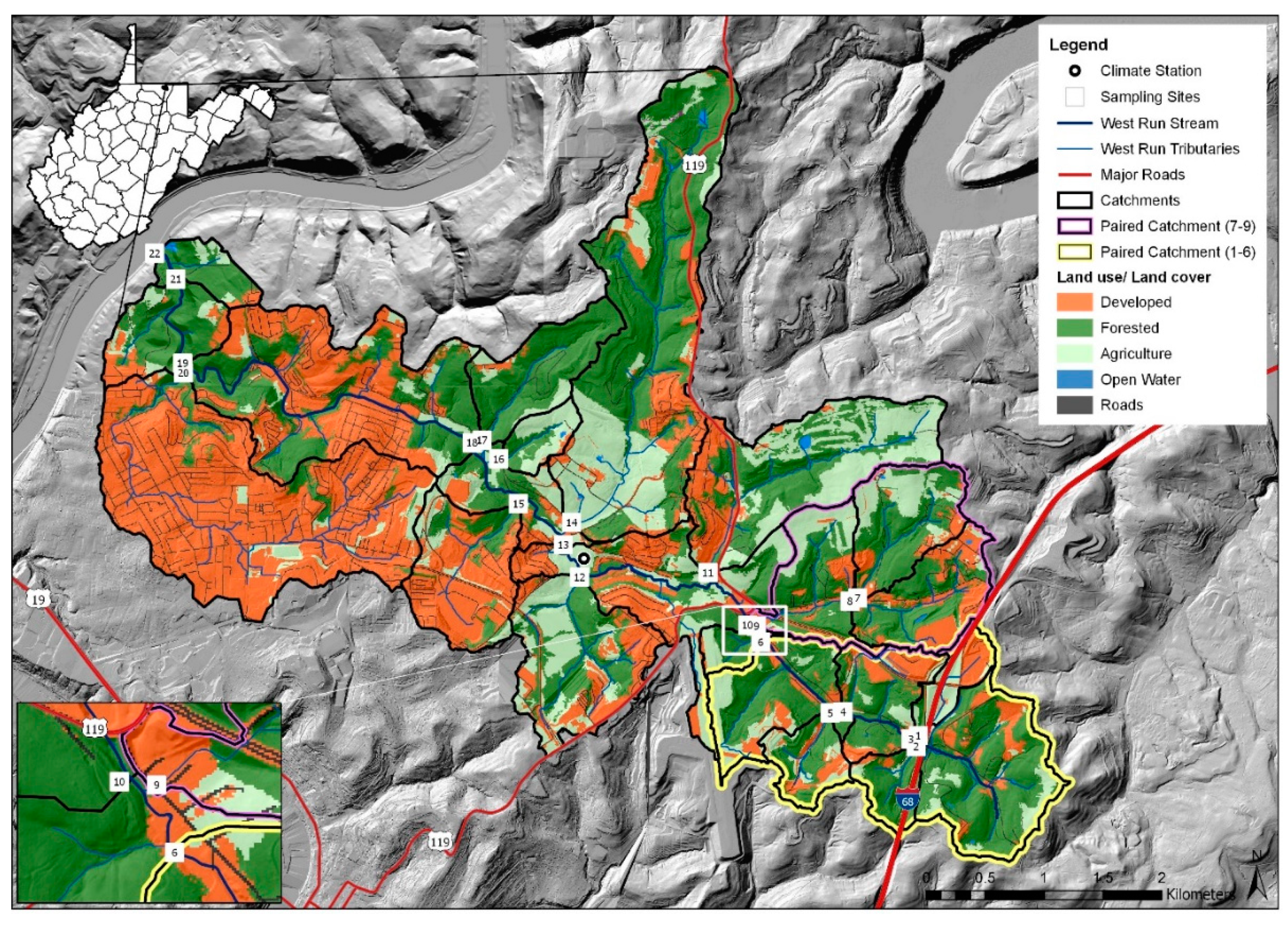
West Run Watershed (WRW) is located in the Monongahela Watershed and is categorized as a Hydrologic Group D watershed (HUC #05020003) located near Morgantown, West Virginia, USA [12]. The watershed spans 23 km2, and the main drainage, West Run Creek, drains directly into the Monongahela River [27,35]. Anecdotally observed by the project managers of the watershed-based plan for West Run of the Monongahela River [52], the increase in urban sprawl stemming from the surrounding city of Morgantown continues to increase the severity and frequency of flooding. The channel of West Run, according to habitat surveys, lacks sinuosity in many reaches and possesses a low channel slope of 1.1%, with back watering (flooding) near the terminus [12,52]. For this reason, site 22 (Figure 1) was excluded from the current study due to potential backwatering with the Monongahela River, and subsequent confounding analyses at that location. The average net radiation in Morgantown, measured during a study by Arguez et al. [53], from 1981 to 2010 was 130.68 W/m2. The average recorded precipitation depth in Morgantown is approximately 1096 mm/year (1981–2010). Precipitation falls throughout the year but increases in quantity during the spring and summer months [54]. Previous studies showed that precipitation has significantly (p = 0.01) increased in the Appalachian region by 2.2% over the past 111 years [27,54,55]. Precipitation is frequently generated via frontal storm convergence systems, but during the summer months in particular, precipitation also occurs via orographic and/or convective processes [12,54,55,56]. Dynamic water parameters (i.e., base flow, Tw, and storm flow) were first monitored in the WRW in 2016 when stilling wells were installed [12], using a paired and nested-scale experimental watershed study design. Each site was equipped with a Solinst Levelogger Gold pressure transducer that logged and stored Tw (°C) data, with an accuracy of ±0.05 °C, and stage (water depth, cm), with an accuracy of ±0.3 cm, at five-minute intervals. During the study period, climate data were recorded using research-grade climate instrumentation located within approximately 100 m of site 13 (Figure 1). Climate variables (recorded at a height of 3 m) included precipitation (TE525 Tipping Bucket Rain Gauge), average air temperature and relative humidity (Campbell Scientific HC2S3 Temperature and Relative Humidity Probe), average wind speed (Met One 034B Wind Set instrument), and net radiation (Campbell Scientific NR01 Four-Component Net Radiation Sensor).
2.2. LULC Data
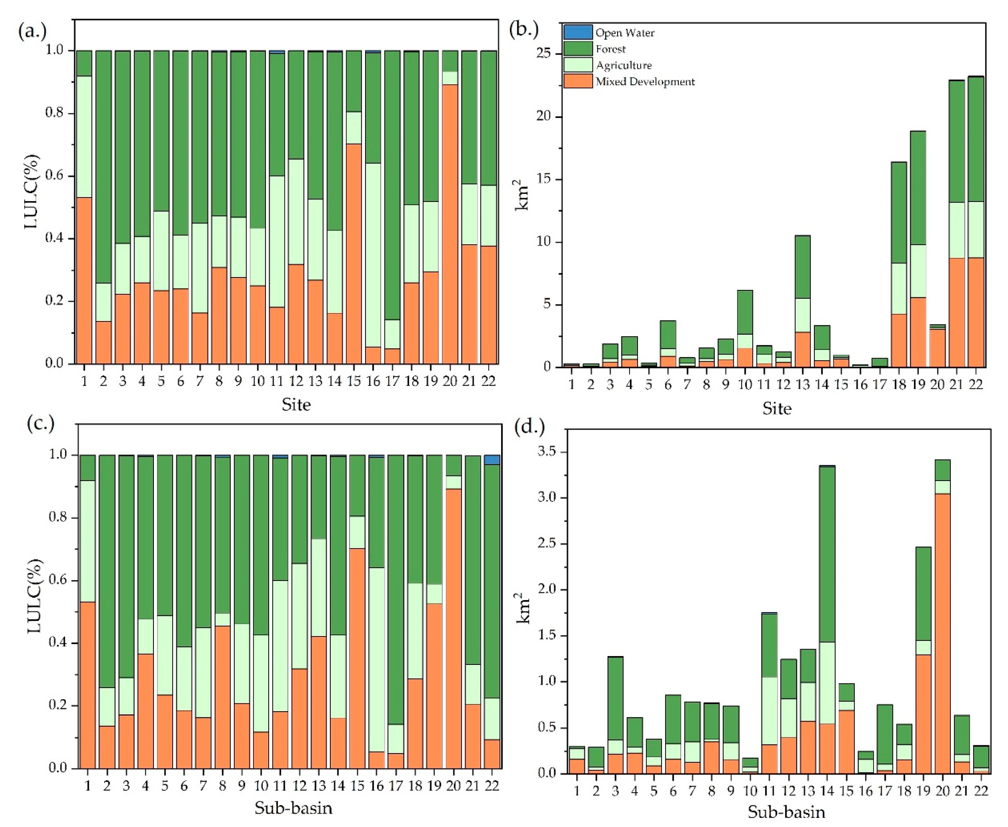
LULC data were derived from National Agricultural Imaging Program (NAIP) 2016 data. Initially, LULC types included 16 different assignations. For the current work, each of the original 16 LULC types was further grouped (lumped) into one of four LULC categories mixed-developed, agriculture, forested, and open water (Table 1). Using Arc GIS, watershed and sub-catchment boundaries were delineated, and LULC data incorporated. Each pixel representing 5 m2 was counted and converted to km2 and used to estimate percent LULC for each sub-catchment draining to each monitoring site; see Table 2 and Figure 2. Overall land use in West Run Watershed assessed using Arc GIS projected a composition of 19.4% agriculture, 42.7% forest, and 37.7% urban/suburban, with the portion of agricultural land use mainly comprised of animal husbandry (i.e., cattle) and crop fields (i.e., corn, soybeans, and cover crops) [12,27]. The presence of different land-use types coupled with regular land-use manipulation via human development justifies WRW categorization as a representative contemporary mixed-land-use watershed [12]. A combination of agricultural, mining, and industrial land use in and surrounding WRW has contributed to ongoing land and water resource degradation [12]. As per The United States Census Bureau report from 2019, the current population of Morgantown is 30,539 [57].
Forested land-use practices are the most abundant land-use classification in the WRW. For the current work, land-use/land-cover types grouped in the forested category included mature vegetation but were separated from mine grass classification, which is assumed to have succeeded to an intermediate successional stage [58,59]. Agricultural land-use practices were those classifications associated with early successional stages (i.e., low vegetation) or agriculturally maintained pastures and fields. The original classification grouped as mixed development land-use practices included mixed-development and all other LULC classifications associated with urban areas and/or impervious surfaces (e.g., barren, roads, and impervious) (Table 1) [34,35,60,61]. Figure 2 shows LULC proportions separated into percent area, and the LULC area of both the individual sites and each individual sub-basin.
2.3. Data Analysis
Data analyses included descriptive statistics (5 min data) of annual, quarterly, and monthly data in 2018 [47]. Quarterly time steps were delineated as 1 January–31 March (quarter 1), 1 April–30 June (quarter 2), 1 July–30 September (quarter 3), and 1 October–31 December (quarter 4). Data postprocessing included estimation of erroneous data or missing points (<0.2% of total data) by averaging between data points on either side of a gap, or by linear interpolation [62]. The Tw data were shown to be non-normally distributed using the Anderson–Darling test [62]. Therefore, land-use areas corresponding to each site were compared to maximum Tw using the Spearman rank correlation coefficient test (α = 0.05). The open water land-use type was excluded from analyses due to its negligible areal coverage relative to other land-use types in the watershed. Three separate analyses were run including (a) all sites (b) tributaries only (i.e., sites 1, 2, 5, 7, 8, 9, 11, 12, 14, 15, 16, 17, and 20), and (c) mainstem West Run Creek only (i.e., sites 3, 4, 6, 10, 13, 18, and 21) to assess the varying effects of surrounding land-use practices on tributaries vs. mainstem sites. Due to the detrimental influence of maximum Tw on aquatic biological/geochemical processes, a pairwise comparison of daily maximum Tw was conducted on a site by site basis using a Kruskal–Wallis ANOVA [62]. Multiple principle component analyses (PCAs) were developed to illustrate the relationship between LULC types at an annual, quarterly, and monthly timescale, again excluding open water [63]. Using OriginPro Pro 9b Academic (OriginLab Corporation, Northampton, MA, USA), correlation biplots were generated with standardized data [63]. Due to the use of observed Tw data, no autoscaling preprocessing was needed to compare Tw and LULC data in the PCA analysis. However, due to the use of differing units (i.e., proportions (%) and temperature (°C)), a correlation matrix was used rather than a covariate matrix [63]. Following the Kaiser–Guttman criterion, eigenvalues greater than one were accepted as principle components above the threshold of importance [63].
3. Results
3.1. Climate during Study
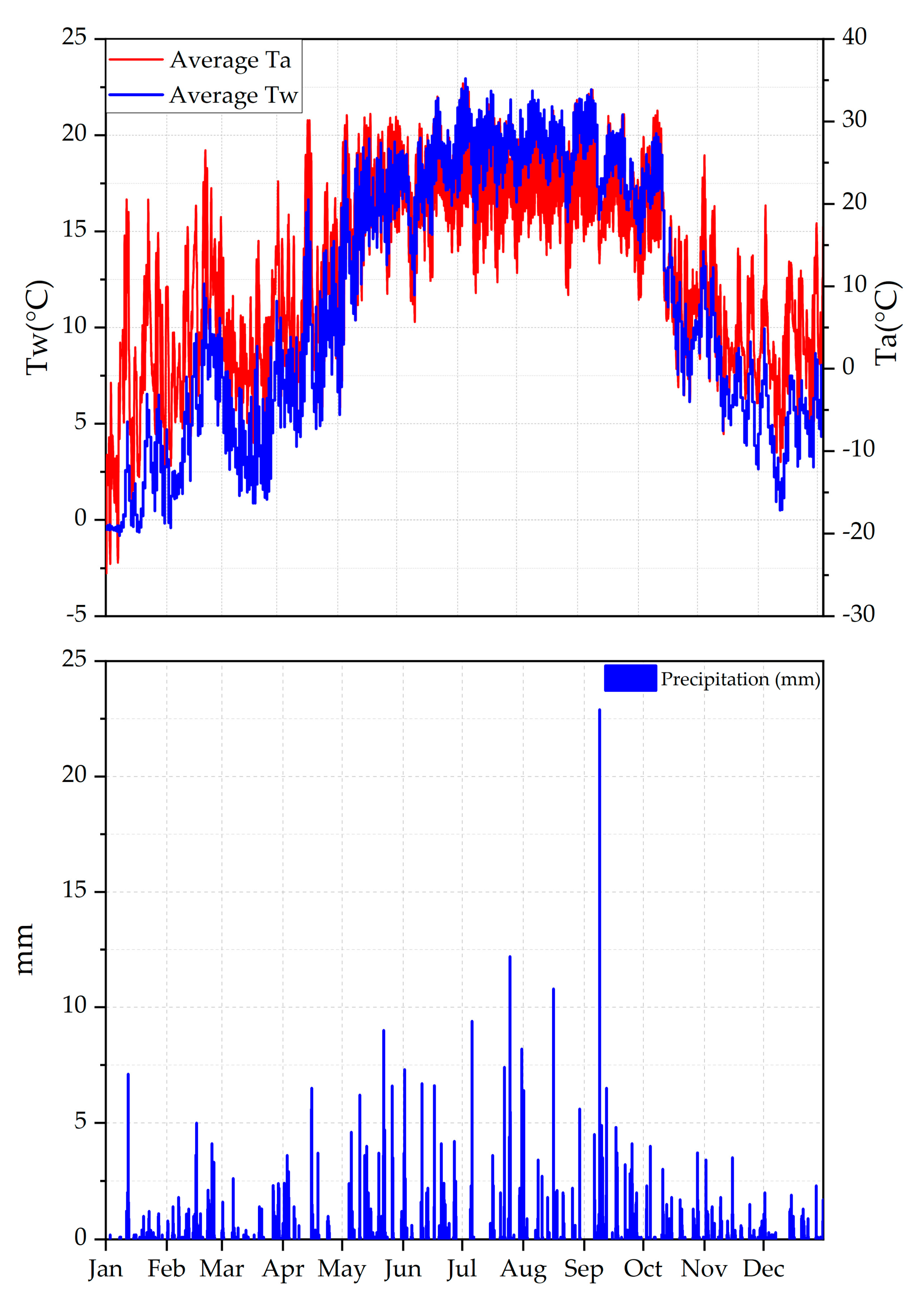
Total precipitation recorded in West Run Watershed in 2018 was 1378 mm, which was 282 mm higher than average annual precipitation (1096 mm) over the previous 111 years [54]. The largest precipitation event (22.9 mm) occurred in a 5 min window on 9 September. The largest continuous precipitation event (83.2 mm) began on 8 September at 18:00 and lasted until 9 September at 16:30; see Figure 3b. Mean air temperature (Ta) in 2018 was 11.6 °C, which was 0.2 °C lower than the average annual temperature (11.4 °C) in West Virginia between 1990 and 2016 [54]. The coldest (−24.8 °C) and warmest (34.6 °C) recorded temperature occurred on January 1st at 8:00 and on 1 July at 17:00, respectively. The maximum net radiation was 1100 W/m2, recorded on 7 May at 12:00. The mean near surface (1.5 m) net radiation was 139.5 W/m2 (Figure 3), which was 8.82 W/m2 higher than the mean annual net radiation in Morgantown between 1981 and 2010 (130.68 W/m2) [53].
3.2. Annual Stream Water Temperature
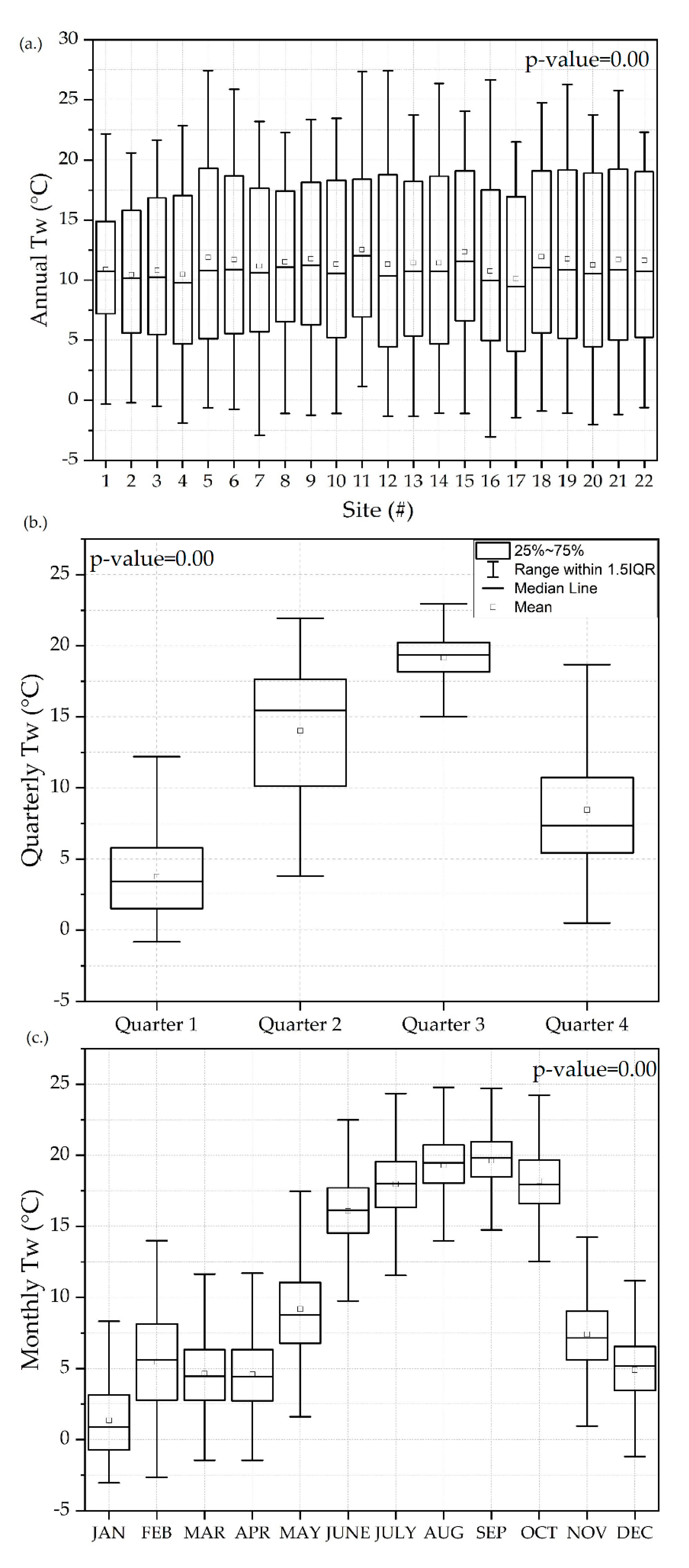
Annual average water temperature (Tw) across all sites varied by 2.4 °C, with a maximum of 12.5 °C at site 11 [dominant LULC agriculture; (41.9%)] and a minimum of 10.1 °C at site 17 [dominant LULC forested; (85.8%)] (Table 3). The lowest recorded Tw (−3.0 °C) occurred at site 16 [dominant LULC agriculture; (58.7%)] at 6:45 on 7 January, and the highest recorded Tw (27.4 °C) occurred at site 5 [dominant LULC forested; (51.1%)] at 16:05 on 3 July. Both were recorded less than a week after the lowest (−24.8 °C) and highest recorded Ta (34.6 °C).
Pairwise comparisons on a site by site basis comparing 21 of the 22 sites indicated that maximum Tw at site 1 was significantly different from site 5 (p = 0.02) [dominant LULC forested; (51.1%)], 11 (p = 0.00) [dominant LULC agriculture; (41.9%)], 12 (p = 0.00) [dominant LULC forested; (34.5%)], and 15 (p = 0.01) [dominant LULC mixed development; (70.3%)] (Table 4). Maximum Tw at site 2 [dominate LULC forested (74.2%)] was significantly different from 5 (p = 0.00) [dominate LULC forested; (51.1%)], 14 (p = 0.00) [dominant LULC forested; (56.9%)], 15 (p = 0.00), 18 (p = 0.00) [dominant LULC forested; (48.9%)], 19 (p = 0.00) [dominant LULC forested; (47.9%)], and 21 (p = 0.00) [dominant LULC forested; (42.2%)]. Maximum Tw at site 3 [dominant LULC forested; (61.3%)] was significantly different from site 5 (p = 0.01), 11 (p = 0.00), 12 (p = 0.00), and 15 (p = 0.01). Maximum Tw at site 4 [dominant LULC forested; (59.0%)] was significantly different from site 5 (p = 0.01), 11 (p = 0.00), 12 (p = 0.00), and 15 (p = 0.01). Maximum Tw at site 5 was significantly different from site 17 (p = 0.00). Maximum Tw at site 17 was significantly different from site 5 (p = 0.00), 6 (p = 0.01), 11 (p = 0.00), 12 (p = 0.00), 14 (p = 0.01), 15 (p = 0.00), 18 (p = 0.01), 19 (p = 0.02), 21 (p = 0.02). Spearman correlation coefficients of all twenty-one sites across the entire annual year indicated a significant (p = 0.01) positive correlation (rs = 0.6) between maximum Tw and agriculture LULC area, and a negative correlation (rs = −0.5) between maximum Tw and Forest LULCs (p = 0.03).
3.3. Quarterly Stream Water Temperature
Seasonal Tw regimes showed that quarter 1 (1 January–31 March) had the lowest minimum Tw (−3.0 °C, site 16), with a mean of 3.2 °C, a maximum Tw of 14.0 °C (site 12), and a standard deviation of 3.8 °C (Table 3, Figure 4). Quarter 2 (1 April–30 June) included the highest standard deviation (4.7 °C), and a mean Tw of 14.6 °C, a maximum Tw of 27.3 °C (site 11), and a minimum Tw of 1.6 °C (site 17). Quarter 3 (1 July–30 September) had the highest mean Tw (19.2 °C) and maximum Tw (27.4 °C) (site 12), with a standard deviation of 2.2 °C, and a minimum of 12.5 °C (site 4). Results from the Kruskal–Wallis ANOVA showed that all 21 sites were significantly different from each other during one of the four quarters based on daily maximum Tw. The most significant differences were observed in quarter 3, with 130 significant differences (all, p ≤ 0.04). Quarter 4 had three significant differences—the lowest number of returned significant differences of all four quarters. All three of the returned significant differences involved site 1 [site 4 (p = 0.01), 5 (p = 0.05), and 17 (p = 0.00)]. Significant Spearman correlation coefficients (α = 0.05) between LULC types and maximum Tw occurred during quarter 1, 3, and 4. Agriculture LULCs showed a significant positive correlation with maximum Tw during quarter 1 (rs = 0.5) (p = 0.03) and quarter 3 (rs = 0.5) (p = 0.01), specifically at sites 1, 11, 12, and 16. Forested LULCs showed a significant negative correlation with maximum Tw during quarter 3 (rs = −0.5) (p = 0.04), specifically at sites 2 and 17.
3.4. Monthly Stream Water Temperature
January included the lowest minimum Tw (−3.0 °C) (site 16), with a standard deviation of 2.4 °C (all 21 sites), a mean Tw of 1.4 °C (All 21 sites), and a maximum of 8.3 °C (site 8) (Table 3). May included the highest standard deviation (3.3 °C), with a mean Tw of 21.8 °C, a maximum of 23.4 °C (site 12), and a minimum of 1.6 °C (site 17). July included the highest maximum Tw (27.4°C) (site 12), with a mean Tw of 16.1 °C, a minimum Tw of 10.3 °C (site 17), and a standard deviation of 2.3 °C. September included the highest mean Tw (19.6 °C), a minimum Tw of 13.2 °C (site 17), a maximum Tw of 27.1 °C (site 16), and a standard deviation of 1.9 °C (Table 3). LULC and Tw analysis (n = 21 sites) showed 12 significant (α = 0.05) correlations with Tw variables. Results from the Kruskal–Wallis ANOVA showed that all 21 sites were significantly different from each other during at least one of the twelve months based on daily maximum Tw. The most significant differences were shown in July, with 108 significant differences (p ≤ 0.04). Both February and October had no significant differences between sites. Significant Spearman correlation coefficients (α = 0.05), between LULC types and maximum Tw, occurred during February, April, June, July, August, September, October, November, and December. Agriculture LULCs showed a significant positive correlation with maximum Tw during February (rs = 0.5) (p = 0.03), June (rs = 0.6) (p = 0.03), August, (rs = 0.7) (p = 0.04), September (rs = 0.7) (p = 0.05), November (rs = 0.8) (p = 0.03), and December (rs = 0.5) (p = 0.05), specifically at sites 1, 11, 12 and 16. Forested LULCs showed a significant negative correlation with maximum Tw during August (rs = −0.9) (p = 0.01), September (rs = −0.9) (p = 0.00), and December (rs = −0.5) (p = 0.02), specifically at sites 2 and 17 (all p values ≤ 0.04). Mixed-development LULCs showed a significant positive correlation with maximum Tw during August, (rs = 0.9) (p = 0.01), September (rs = 0.9) (p = 0.00), and November (rs = 0.6) (p = 0.04) at sites 1, 8, 12, 15, and 20.
3.5. PCAs
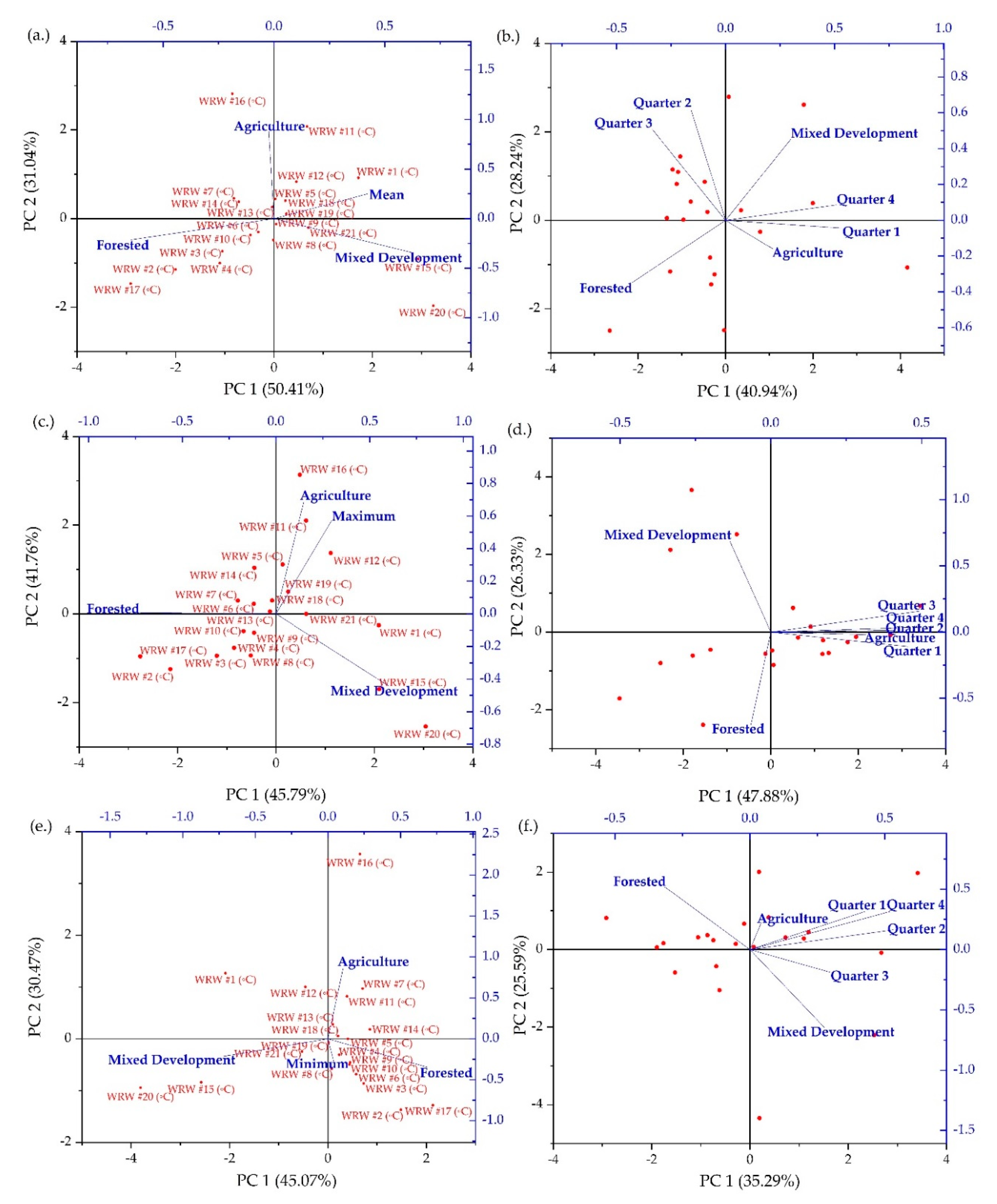
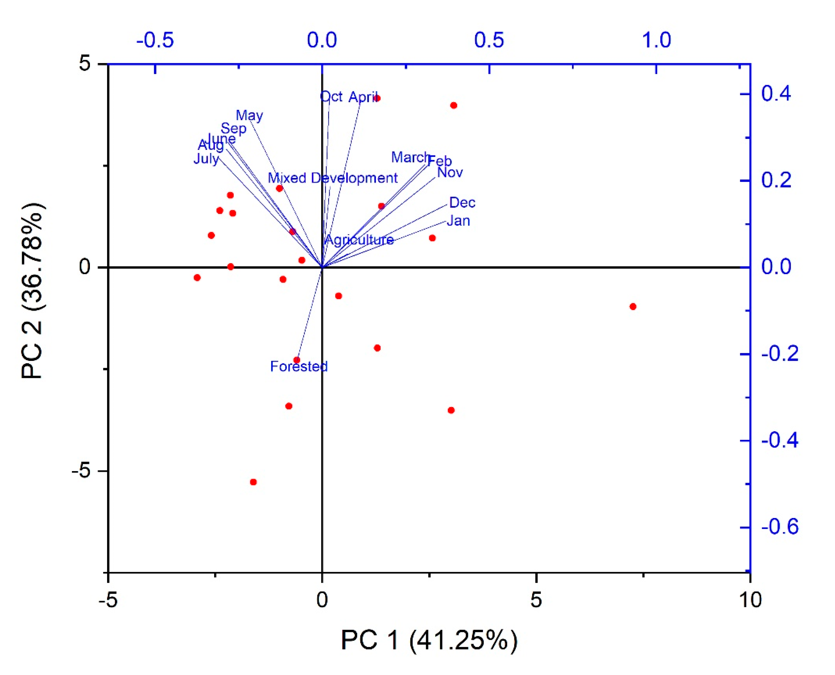
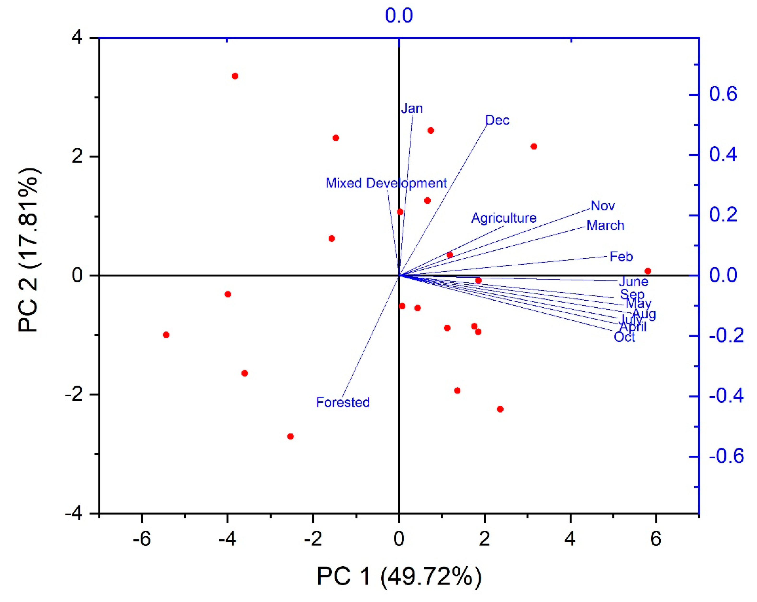
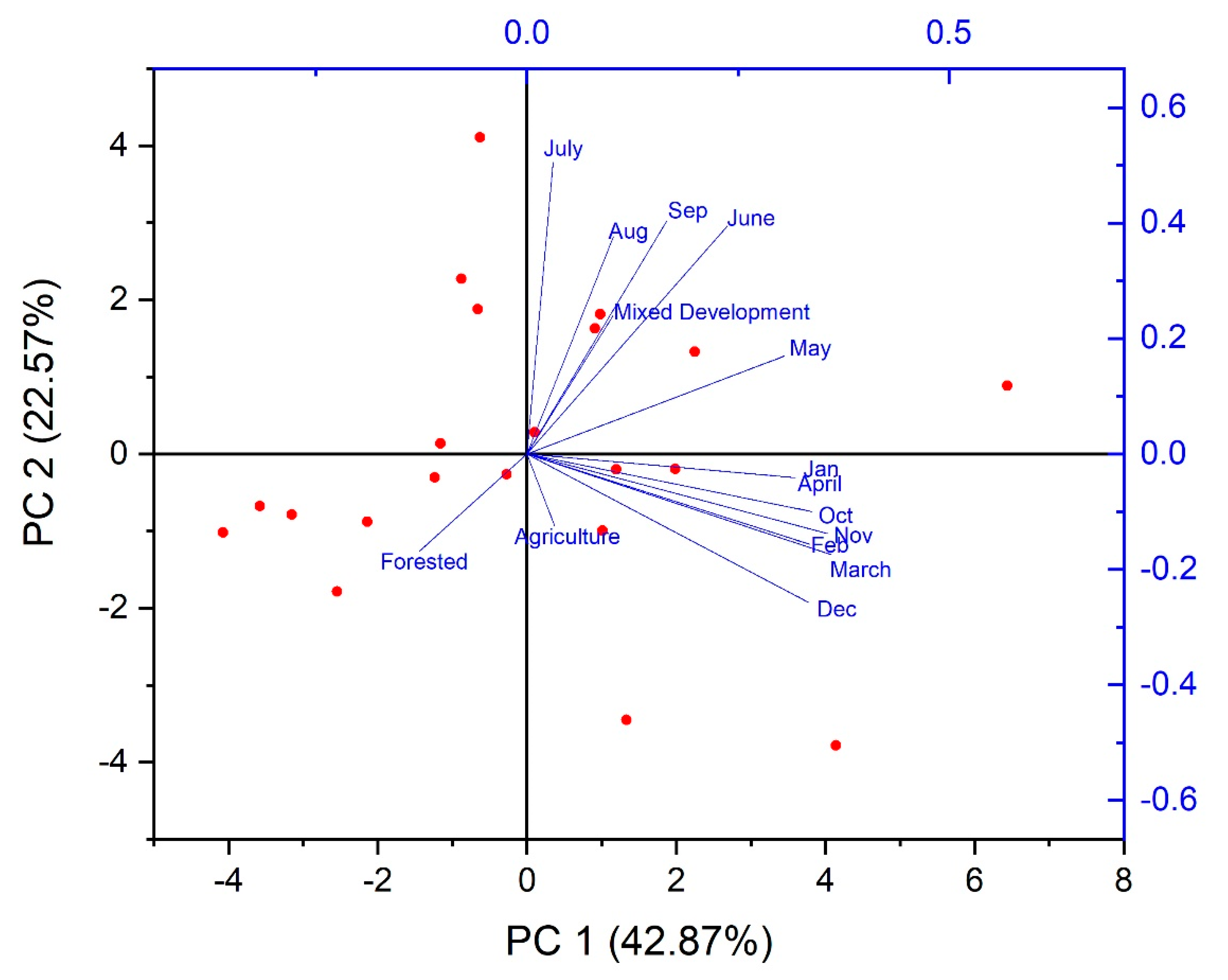
Annual timeseries comparisons between LULC areas and Tw variables at site 1–21 all showed two eigenvalues above the threshold of importance. If all variables (n = 4) exerted equal influence for the annual PCA, the values would be 0.5 (i.e., √(1/n)) [63]. For mean Tw annual PCA, PC1 had an eigenvalue of 2.0 and explained 50.4% of the variance and PC2 had an eigenvalue of 1.2 and explained 31.0% of the variance. PC1 was comprised of a positive relationship between mean Tw and mixed-development LULC and a negative relationship with forested LULC. PC2 was comprised of a positive relationship between agricultural LULC and mean Tw. For the minimum Tw annual PCA, PC1 had an eigenvalue of 1.8 and explained 45.1% of the variance and PC2 had an eigenvalue of 1.2 and explained 30.5% of the variance. PC1 was comprised of a negative correlation between minimum Tw and mixed-development LULC and a positive relationship with forested LULC. PC2 had a positive relationship between agricultural LULC and minimum Tw. For the maximum Tw annual PCA, PC1 had an eigenvalue of 1.8 and explained 45.8% of the variance and PC2 had an eigenvalue of 1.7 and explained 41.8% of the variance. PC1 was comprised of a positive relationship between maximum Tw and mixed-development LULC and a negative relationship with forested LULC. PC2 was comprised of a positive relationship between agricultural LULC and maximum Tw. Mean and maximum quarterly timeseries comparisons between LULC areas showed three eigenvalues above the threshold of importance. The mean Tw quarterly timeseries comparisons between LULC areas showed two eigenvalues above the threshold of importance. If all variables (n = 7) exerted equal influence, the eigenvalues would equal 0.38. For the mean Tw quarterly PCA, PC1 had an eigenvalue of 2.9 and explained 40.9% of the variance and PC2 had an eigenvalue of 2.0 and explained 28.4% of the variance. PC1 had a positive relationship between mixed-development LULC and quarter 1, and a negative relationship with forested LULC. PC2 was comprised of a positive relationship between mixed-development LULCs and quarters 2 and 3. For the minimum Tw quarterly PCA, PC1 had an eigenvalue of 2.5 and explained 35.3% of the variance and PC2 had an eigenvalue of 1.8 and explained 25.6% of the variance. PC1 showed a positive relationship between mixed-development LULC and quarter 1, 2 and 4, and a negative relationship with forested LULC. PC2 showed a positive relationship between mixed-development LULC and quarters 1 and 4, and a negative relationship with forested LULC. For the maximum Tw quarterly PCA, PC1 had an eigenvalue of 3.4 and explained 47.9% of the variance and PC2 had an eigenvalue of 1.8 and explained 26.3% of the variance. PC1 was comprised of a positive relationship between agricultural LULC and quarter 1, 2 and 4. PC2 was comprised of a positive relationship between mixed-development LULC and a negative relationship with forested LULC during quarter 4. Monthly timeseries comparison between LULC areas and Tw variables all showed four eigenvalues above the threshold of importance. If all variables (n = 15) exerted equal influence, the eigenvalues would equal 0.26. For the mean Tw monthly PCA, PC1 had an eigenvalue of 6.2 and explained 41.3% of the variance and PC2 had an eigenvalue of 5.5 and explained 36.8% of the variance. For the minimum Tw monthly PCA, PC1 had an eigenvalue of 6.4 and explained 42.9% of the variance and PC2 had an eigenvalue of 3.4 and explained 22.6% of the variance. For the maximum Tw monthly PCA, PC1 had an eigenvalue of 7.5 and explained 49.7% of the variance and PC2 had an eigenvalue of 2.7 and explained 17.8% of the variance. Extracted Eigenvector coefficients and plots for each monthly principle component analysis are included in the Appendix (Table A1, Table A2 and Table A3, Figure A1, Figure A2 and Figure A3).
4. Discussion
4.1. Climate during Study
Climate variables (e.g., Ta, precipitation, and net radiation) recorded in West Run Watershed in 2018 were average relative to historic climatic trends of West Virginia (i.e., 1900–2016) [54]. The average mean temperature (11.6 °C) differed only slightly (1.7%) from historic (1900–2016) averages observed in West Virginia from 1900 to 2016 (11.4 °C). During the study period, there was above average (20.5% higher) total precipitation relative to the historic (1900–2016) average (1096 mm) [54,64]. WRW did not include a dry season in 2018 and, a majority of the total precipitation fell during quarters 2 and 3 [46]. The overall climate in WRW during 2018 was predictably variable and consistent with historic climate trends (Figure 3) [46].
4.2. Stream Water Temperature
The highest maximum (27.4 °C) Tw was recorded during quarter 3, specifically for July. This is expected given the seasonal climate of WRW, which has the highest recorded Ta (34.6 °C) during July. While the highest Ta and Tw were recorded during quarter 3, the highest mean Ta was recorded during July, and the highest mean Tw was recorded during September (19.6 °C). In quarter 2, May had the highest Tw standard deviation (3.3 °C) (Figure 4) [64]. Further analysis into the Tw and Ta trends (Figure 3) showed that Tw followed but lagged behind Ta during May and across the entire study period [65,66,67,68]. This trend is constant with results of past studies that showed a strong relationship between Tw and Ta [39,66,67]. In May, Ta had a high standard deviation compared to other months (6.2 °C). The high Tw standard deviation in quarter 2 and May is likely attributable to the close relationship between Ta and Tw, as shown in many previous studies [38,39,66,67].
4.3. Stream Water Temperature LULC Relations
In general, results from both the PCA (Figure 5) and the Spearman rank correlation coefficient test (Table 5) showed that an increase in the proportion of forested LULC types is negatively correlated with all Tw variables, as confirmed in previous studies [14,22,65]. These results follow the same conclusions made by previous researchers that showed that forest harvest (e.g., clear cuts/canopy removal) increases Tw [6,14,16,22]. Additionally, although not surprising, during the winter season, a positive correlation was observed between the proportion of forest LULC and minimum Tw.
Moore et al. [14] suggested that riparian vegetation insolates Tw by lowering convective heat loss to the above atmosphere, thereby cooling Tw in the summer and warming Tw in the winter via latent heat gain [15,23,68]. In the current work, positive correlations between maximum Tw and percent forest LULC were observed in specific tributaries (Figure 6), thus contradicting findings of previous research [6,65,68]. However, when sites 8 and 9 were removed from the data pool, correlations trends reverted to the expected negative correlation [6,65]. For sites 8 and 9 of the current work, the positive correlation may be attributed to the high proportion of directly adjacent mixed-development LULC types at both sites 8 and 9 prior to monitoring sites.
Results from both the PCA (Figure 5) analyses and the Spearman rank correlation coefficient test (Table 5) showed that mixed-development LULC types were significantly correlated with mean, minimum, and maximum Tw, with variable effects throughout the year [30,31,32,34,35,60,61]. While results of the mixed-development Tw analysis were similar to results of previous research, the current work provides important validation by means of the high number of sampling sites and high frequency sampling [32,34,47]. Interestingly, PCA results showed a negative correlation between minimum, maximum, and mean Tw during the winter and early spring months (i.e., January, February, March, April, November, and December), indicating overall lower Tw. These findings contradict results of other research analyzing the relationship between mixed-development LULC and Tw. Rice et al. [34] showed that mean Tw increased during the winter season in heavily urbanized catchments of Boone, North Carolina. Alternatively, to Rice et al. [34], lower Tw correlated with mixed development during cooler months (i.e., January, February, March, April, November, and December) could be explained by runoff from impervious surfaces, which during these months is often lower in temperature than the Tw of surrounding streams. Qun et al. [69] showed a negative correlation between urban impervious surface and land surface temperatures (i.e., lower surface temperatures) during winter daytimes. Conflicting results might be further explained by the complex physiographic mosaic of the study watershed in which mixed development LULC types are broken up by other forested and agricultural LULC types at varying relative positions on the landscape, thus leaving room for future investigations.
Agricultural LULC types had a positive Spearman correlation, with maximum Tw in every quarter and month, except January (Table 5). These findings may be, at least in part, due to the removal of riparian vegetation, increased subsurface lateral flow rates through drainage tiles, and/or increased soil shortwave radiation exposure during periods when fields are bare as per findings of previous literature [27,70]. Interestingly, a relationship appeared between maximum Tw and crop absence. Typically, in the study watershed, crops are planted in spring and harvested in middle to late July following the observed trend in Table 5. Therefore, the positive relationship between crop absence and maximum Tw could be explained, at least in part, by increased shortwave interception and reduce runoff volumes through evapotranspiration and interception of precipitation by crops [15,23]. Conversely, after harvest, the relationship becomes significant because runoff volumes increase and the soil is exposed to greater amounts of shortwave radiation thereby reaching higher temperatures [15,27,29]. Furthermore, during these periods, water contacting or infiltrating into the soil is heated and transported to surrounding streams via runoff or subsurface lateral flows [27]. Younus et al. [27] found that drainage tiles exacerbated transport of heated subsurface lateral flow into surrounding streams during irrigation or precipitation events. The agricultural fields in the current study watershed have drainage tiles installed. Thus, subsurface lateral flows to West Run Creek may be increased, further explaining the significant relationship between maximum Tw and agricultural LULC types.
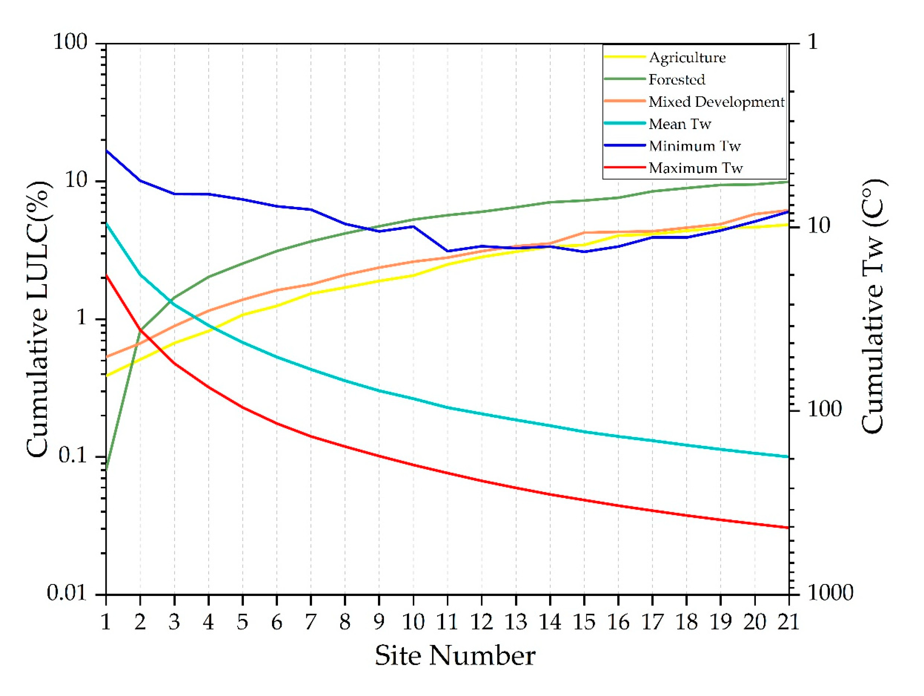
4.4. LULC Tw Tipping Points
Forested LULC types influenced Tw most significantly in the current investigation (Figure 6). As the percent of forested LULC types decreased below 74.2%, associated maximum Tw began to increase (thus a potential tipping point). As the percent of forested LULC decreased below 61.1% mean Tw began to either increase or decrease depending on the time of year. Below 52.2% forested LULC, the minimum Tw of associated streams began to increase or decrease again depending on the time of year. Mixed-development LULC types had next greatest impacts on Tw.
As the percent of mixed-development LULC types increased above 14%, associated mean Tw increased (thus a potential mixed-development tipping point). Above 24.1% mixed development, maximum Tw began to either increase or decrease depending on the time of year, and above 26.8% mixed development, the minimum Tw of streams began to increase or decrease (depending on the time of year). Agricultural LULC types also influenced Tw significantly. As the percent of agriculture LULC types increased above 14.9%, associated maximum Tw began to increase. Above 16.0% agriculture LULC, mean Tw began to increase, and above 26.4% agriculture LULC, the minimum stream Tw began to increase or decrease (time of year dependent).
4.5. Study Implications and Future Directions
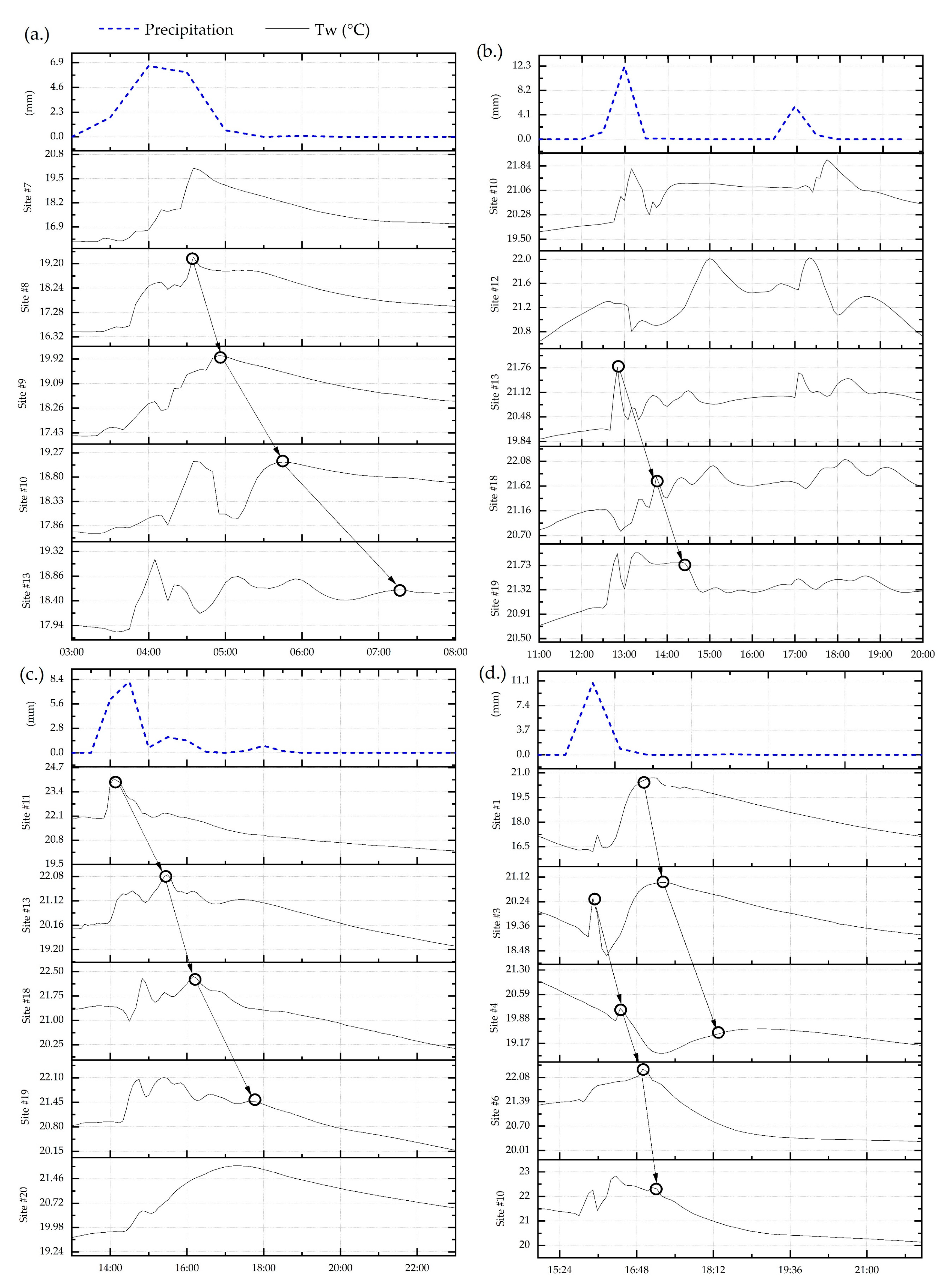
Implementing the nested experimental watershed study design coupled with the high-temporal and spatial-sampling regime used in this work allowed for a more comprehensive evaluation of surrounding LULC effects on associated Tw than is normally found in the primary literature. Forested LULC types were associated with overall lower Tw, whereas both mixed-development and agriculture LULC types had higher overall Tw. The finding of LULC tipping points (thresholds) for all three of the analyzed LULC classifications provides valuable information for both land managers and policy makers. For example, Tw tipping points emerged as forested LULC types dropped below 74.2%, due to the conversion to mixed development or agricultural LULC types. These tipping points can be used to guide management decisions in terms of development limits. Given the importance of maximum Tw for stream biota, a preliminary analysis of thermal surges was conducted. Select summer precipitation events were assessed as per Zeiger and Hubbart [32], Rice et al. [34], and Anderson et al. [71], where a Tw surge is defined as a greater than 1.0 °C increase within a 15 min time interval. Figure 7 is a stacked comparison of Tw on the y-axis and time on the x-axis showing time lag from the related precipitation event. Successive sites were added to Figure 7, showing the thermal plume moving through the watershed and eventually dissipating. Although this analysis was preliminary, it showed the existence of these events, thus conveying the need for future research into thermal surge dynamics. Future investigations may benefit from additional monitoring years to better understand the importance of climate and antecedent conditions with regard to Tw processes. In addition, future studies could focus on minimum Tw and mean Tw, and perhaps Tw variance, to understand relationships between land use, climate change and Tw regimes.
5. Conclusions
No previous research investigating stream water temperature (Tw) in contemporary watersheds has used such a high-temporal and spatial-sampling regime as that included in the current investigation. Implementation of the experimental design used in the current research is necessary to provide both validation for previous results and the discovery of temporal variation in LULC characteristics influencing Tw. In the current work, the relationship between LULC types and Tw was investigated in the Appalachian region of the eastern United States. The analysis used five-minute Tw timeseries data collected at 22-site nested sites using an experimental watershed study design. Results indicated that LULC has varying effects on Tw both spatially and temporally. PCA results showed that forested LULC types typically lowered maximum and mean Tw, particularly in the late summer months, whereas Spearman correlation results showed significant (p = 0.01) negative correlations with maximum Tw (−0.9) during August and September. PCA results indicated that mixed-development LULC types typically increased maximum and mean Tw during the summer months, whereas Spearman correlation results showed significant (p = 0.00) positive correlation with maximum Tw (0.9) during August and September. PCA results showed that agriculture LULC types were correlated with maximum Tw in every month except January. Although results are specific to the study watershed, the finding of tipping points shows LULC thresholds that, when exceeded, may begin to impact associated Tw. These relationships likely exist in all watersheds, particularly contemporary (municipal) watersheds. Given the impact that maximum Tw can have on stream ecosystems, a preliminary investigation of thermal surge events was conducted. This investigation showed thermal surges in the study watershed, and therefore presents future research opportunities into the investigation of Tw surge dynamics. Both results and findings of this study will advance the decision-making success of land managers and policy makers concerned with the health of aquatic ecosystems. In particular, the high-resolution (n = 22) study design presented in this work facilitates identification of upland mitigation sites and corresponding greater certainty in fiscal investment outcomes.
Author Contributions
Conceptualization, J.A.H.; methodology, J.A.H.; formal analysis, J.P.H. and J.A.H.; investigation, J.A.H. and J.P.H.; resources, J.A.H.; data curation, J.A.H.; writing—original draft preparation, J.A.H. and J.P.H.; writing—review and editing, J.A.H. and J.P.H.; visualization, J.A.H. and J.P.H.; supervision, J.A.H.; project administration, J.A.H.; funding acquisition, J.A.H. The authors declare no conflict of interest for the current work. All authors have read and agreed to the published version of the manuscript.
Funding
This work was supported by the National Science Foundation under Award Number OIA−1458952, the USDA National Institute of Food and Agriculture, Hatch project accession number 1011536, and the West Virginia Agricultural and Forestry Experiment Station. Results presented may not reflect the views of the sponsors and no official endorsement should be inferred. The funders had no role in study design, data collection and analysis, decision to publish, or preparation of the manuscript.
Acknowledgments
Special thanks are due to the many scientists of the Interdisciplinary Hydrology Laboratory (https://www.researchgate.net/lab/The-Interdisciplinary-Hydrology-Laboratory-Jason-A-Hubbart), and the Institute of Water Security and Science (https://iwss.wvu.edu/). The authors also appreciate the feedback of anonymous reviewers whose constructive comments improved the article.
Conflicts of Interest
The authors declare no conflict of interest for the current work.
Appendix A
Figure A1.
Results of the principle component analysis, showing biplots of the extracted principle components of mean monthly water temperature data collected in 2018 at the 22 monitoring sites of West Run Watershed, WV, USA, and their corresponding LULC area (km2).
Figure A1.
Results of the principle component analysis, showing biplots of the extracted principle components of mean monthly water temperature data collected in 2018 at the 22 monitoring sites of West Run Watershed, WV, USA, and their corresponding LULC area (km2).


Table A1.
Coefficients of principal components comprising 15 variables used to define 15 principal components of mean monthly water temperature data in 2018 in West Run Watershed, WV, USA.
Table A1.
Coefficients of principal components comprising 15 variables used to define 15 principal components of mean monthly water temperature data in 2018 in West Run Watershed, WV, USA.
| Variables | Coefficients of PC1 | Coefficients of PC2 | Coefficients of PC3 | Coefficients of PC4 |
|---|---|---|---|---|
| Jan | 0.37 | 0.11 | 0.04 | 0.07 |
| Feb | 0.31 | 0.24 | 0.14 | 0.13 |
| March | 0.32 | 0.24 | 0.06 | 0.04 |
| April | 0.12 | 0.39 | 0.12 | 0.08 |
| May | −0.21 | 0.34 | −0.03 | 0.08 |
| June | −0.28 | 0.29 | 0.02 | 0.04 |
| July | −0.31 | 0.25 | 0.15 | −0.03 |
| Aug | −0.29 | 0.27 | 0.15 | −0.05 |
| Sep | −0.28 | 0.29 | 0.03 | −0.04 |
| Oct | 0.02 | 0.39 | 0.08 | 0.14 |
| Nov | 0.34 | 0.21 | 0.02 | 0.04 |
| Dec | 0.37 | 0.15 | 0.05 | −0.01 |
| Mixed Development | 0.02 | 0.19 | −0.72 | −0.02 |
| Agriculture | 0.08 | 0.03 | 0.39 | −0.80 |
| Forested | −0.08 | −0.22 | 0.49 | 0.55 |
Figure A2.
Results of the principle component analysis, showing biplots of the extracted principle components of maximum monthly water temperature data collected in 2018 at the 22 monitoring sites of West Run Watershed, WV, USA, and their corresponding LULC area (km2).
Figure A2.
Results of the principle component analysis, showing biplots of the extracted principle components of maximum monthly water temperature data collected in 2018 at the 22 monitoring sites of West Run Watershed, WV, USA, and their corresponding LULC area (km2).

Table A2.
Coefficients of principal components comprising 15 variables used to define 15 principal components of maximum monthly water temperature data in 2018 in West Run Watershed, WV, USA.
Table A2.
Coefficients of principal components comprising 15 variables used to define 15 principal components of maximum monthly water temperature data in 2018 in West Run Watershed, WV, USA.
| Variables | Coefficients of PC1 | Coefficients of PC2 | Coefficients of PC3 | Coefficients of PC4 |
|---|---|---|---|---|
| Jan | 0.02 | 0.53 | 0.23 | 0.10 |
| Feb | 0.30 | 0.06 | 0.29 | 0.13 |
| March | 0.27 | 0.16 | 0.15 | 0.02 |
| April | 0.32 | −0.16 | 0.12 | 0.16 |
| May | 0.33 | −0.10 | −0.18 | 0.08 |
| June | 0.32 | −0.02 | 0.02 | 0.24 |
| July | 0.32 | −0.14 | −0.13 | 0.00 |
| Aug | 0.34 | −0.12 | −0.17 | −0.06 |
| Sep | 0.31 | −0.07 | −0.17 | −0.29 |
| Oct | 0.31 | −0.18 | −0.06 | −0.16 |
| Nov | 0.28 | 0.22 | 0.05 | 0.33 |
| Dec | 0.13 | 0.50 | 0.16 | 0.08 |
| Mixed Development | −0.02 | 0.28 | −0.63 | 0.17 |
| Agriculture | 0.15 | 0.17 | 0.29 | −0.73 |
| Forested | −0.08 | −0.40 | 0.46 | 0.30 |
Figure A3.
Results of the principle component analysis, showing biplots of the extracted principle components of minimum monthly water temperature data collected in 2018 at the 22 monitoring sites of West Run Watershed, WV, USA, and their corresponding LULC area (km2).
Figure A3.
Results of the principle component analysis, showing biplots of the extracted principle components of minimum monthly water temperature data collected in 2018 at the 22 monitoring sites of West Run Watershed, WV, USA, and their corresponding LULC area (km2).

Table A3.
Coefficients of principal components comprising 15 variables used to define 15 principal components of minimum monthly water temperature data in 2018 in West Run Watershed, WV, USA.
Table A3.
Coefficients of principal components comprising 15 variables used to define 15 principal components of minimum monthly water temperature data in 2018 in West Run Watershed, WV, USA.
| Variables | Coefficients of PC1 | Coefficients of PC2 | Coefficients of PC3 | Coefficients of PC4 |
|---|---|---|---|---|
| Jan | 0.30 | −0.04 | 0.26 | −0.22 |
| Feb | 0.34 | −0.16 | 0.07 | −0.04 |
| March | 0.36 | −0.17 | −0.08 | −0.01 |
| April | 0.32 | −0.04 | 0.00 | −0.03 |
| May | 0.31 | 0.17 | −0.03 | −0.08 |
| June | 0.24 | 0.40 | 0.02 | −0.10 |
| July | 0.03 | 0.51 | 0.14 | 0.10 |
| Aug | 0.10 | 0.38 | 0.31 | 0.27 |
| Sep | 0.17 | 0.40 | 0.16 | 0.01 |
| Oct | 0.34 | −0.10 | 0.01 | 0.08 |
| Nov | 0.36 | −0.14 | 0.09 | 0.00 |
| Dec | 0.33 | −0.26 | −0.09 | 0.09 |
| Mixed Development | 0.10 | 0.24 | −0.62 | −0.20 |
| Agriculture | 0.03 | −0.12 | 0.06 | 0.82 |
| Forested | −0.13 | −0.17 | 0.61 | −0.34 |
References
- Webb, B.W.; Hannah, D.M.; Moore, R.D.; Brown, L.E.; Nobilis, F. Recent advances in stream and river temperature research. Hydrol. Process. 2008, 918, 902–918. [Google Scholar] [CrossRef]
- Caissie, D. The thermal regime of rivers: A review. Freshw. Biol. 2006, 51, 1389–1406. [Google Scholar] [CrossRef]
- Webb, B.W. Trends in stream and river temperature. Hydrol. Process. 1996, 10, 205–226. [Google Scholar] [CrossRef]
- Coutant, C.C. Perspectives on Temperature in the Pacific Northwest’s Fresh Waters; Oak Ridge National Laboratory: Oak Ridge, TN, USA, 1999. [Google Scholar]
- Winder, M.; Sommer, U. Phytoplankton response to a changing climate. Hydrobiologia 2012, 698, 5–16. [Google Scholar] [CrossRef]
- Pollock, M.M.; Beechie, T.J.; Liermann, M.; Bigley, E.R. Stream Temperature Relationships to Forest Harvest in the Olympic Peninsula. Fish. Sci. 2009, 45, 1–33. [Google Scholar]
- Petty, J.T.; Thorne, D.; Huntsman, B.M.; Mazik, P.M. The temperature-productivity squeeze: Constraints on brook trout growth along an Appalachian river continuum. Hydrobiologia 2014, 727, 151–166. [Google Scholar] [CrossRef]
- Martin, R.W.; Petty, J.T. Local stream temperature and drainage network topology interact to influence the distribution of smallmouth bass and brook trout in a Central appalachian watershed. J. Freshw. Ecol. 2009, 24, 497–508. [Google Scholar] [CrossRef] [Green Version]
- Petty, J.T.; Hansbarger, J.L.; Huntsman, B.M.; Mazik, P.M. Brook trout movement in response to temperature, flow, and thermal refugia within a complex Appalachian riverscape. Trans. Am. Fish. Soc. 2012, 141, 1060–1073. [Google Scholar] [CrossRef]
- Poole, G.C.; Berman, C.H. An ecological perspective on in-stream temperature: Natural heat dynamics and mechanisms of human-caused thermal degradation. Environ. Manag. 2001, 27, 787–802. [Google Scholar] [CrossRef]
- Borman, M.; Larson, L. A case study of river temperature response to agricultural land use and environmental thermal patterns. J. Soil Water Conserv. 2003, 58, 8–12. [Google Scholar]
- Kellner, E.; Hubbart, J.; Stephan, K.; Freedman, Z.; Kutta, E.; Kelly, C.; Morrissey, E. Characterization of sub-watershed-scale stream chemistry regimes in an Appalachian mixed-land-use watershed. Environ. Monit. Assess. 2018, 190. [Google Scholar] [CrossRef] [PubMed]
- Mustafa, M.; Barnhart, B.; Babbar-Sebens, M.; Ficklin, D. Modeling landscape change effects on stream temperature using the Soil and Water Assessment Tool. Water Switz. 2018, 10, 1–18. [Google Scholar] [CrossRef] [Green Version]
- Moore, R.D.; Spittlehouse, D.L.; Story, A. Riparian microclimate and stream temperature response to forest harvesting: A review. J. Am. Water Resour. Assoc. 2005, 7, 813–834. [Google Scholar] [CrossRef]
- Oke, T.R. Boundary Layer Climates, 2nd ed.; Routledge: London, UK, 1987; ISBN 0-203-71545-4. [Google Scholar]
- Gravelle, J.A.; Link, T.E. Influence of timber harvesting on headwater peak stream temperatures in a northern Idaho watershed. (Special issue: Science and management of forest headwater streams). For. Sci. 2007, 53, 189–205. [Google Scholar]
- Webb, B.W.; Zhang, Y. Water temperatures and heat budgets in Dorset chalk water courses. Hydrol. Process. 1999, 321, 309–321. [Google Scholar] [CrossRef]
- Webb, B.W.; Zhang, Y. Spatial and Seasonal Variablility in the Componeets of The River Heat Budget. Hydrol. Process. 1997, 11, 79–101. [Google Scholar] [CrossRef]
- Bulliner, E.; Hubbart, J.A. An improved hemispherical photography model for stream surface shortwave radiation estimations in a central U.S. hardwood forest. Hydrol. Process. 2013, 27, 3885–3895. [Google Scholar] [CrossRef]
- Imhoff, M.L.; Zhang, P.; Wolfe, R.E.; Bounoua, L. Remote sensing of the urban heat island effect across biomes in the continental USA. Remote Sens. Environ. 2010, 114, 504–513. [Google Scholar] [CrossRef] [Green Version]
- Johnson, R.K.; Almlöf, K. Adapting boreal streams to climate change: Effects of riparian vegetation on water temperature and biological assemblages. Freshw. Sci. 2016, 35, 984–997. [Google Scholar] [CrossRef]
- Johnson, S.L.; Jones, J.A. Stream temperature responses to forest harvest and debris flows in western Cascades, Oregon. Can. J. Fish. Aquat. Sci. 2011, 57, 30–39. [Google Scholar] [CrossRef]
- Xuhui, L. Fundamentals of Boundary-Layer Meteorology; Springer: Gewerbestrasse, Switzerland, 2018; ISBN 978-3-319-60851-8. [Google Scholar]
- Boyde, C. Water Quality: An Introduction; Springer: Gewerbestrasse, Switzerland, 2016; ISBN 978-3-319-70548-4. [Google Scholar]
- Petersen, F.; Hubbart, J.A.; Kellner, E.; Kutta, E. Land-use-mediated Escherichia coli concentrations in a contemporary Appalachian watershed. Environ. Earth Sci. 2018, 77, 1–13. [Google Scholar] [CrossRef]
- Wiebe, K.D.; Gollehon, N.R. Agricultural Resources and Environmental Indicators; Nova Publishers: Hauppauge, NY, USA, 2007; ISBN 978-1-60021-467-7. [Google Scholar]
- Younus, M.; Hondzo, M.; Engel, B.A. Stream Temperature Dynamics in Upland Agricultural Watersheds. J. Environ. Eng. 2000, 126, 518–526. [Google Scholar] [CrossRef]
- Campbell, G.S.; Norman, J.M. Introduction to Environmental Biophysics, 2nd ed.; Springer: New York, NY, USA, 1998; ISBN 978-0-387-94937-6. [Google Scholar]
- Hatfield, J.L.; Sauer, T.J.; Prueger, J.H. Managing Soils to Achieve Greater Water Use Efficiency: A Review. Agron. J. 2001, 93, 10. [Google Scholar] [CrossRef]
- Kinouchi, T.; Yagi, H.; Miyamoto, M. Increase in stream temperature related to anthropogenic heat input from urban wastewater. J. Hydrol. 2007, 335, 78–88. [Google Scholar] [CrossRef]
- Palmer, M.A.; Nelson, K.C. Stream Temperature Surges under Urbanization. J. Am. Water Resour. Assoc. 2007, 43, 440–452. [Google Scholar] [CrossRef]
- Zeiger, S.J.; Hubbart, J.A. Urban Stormwater Temperature Surges: A Central US Watershed Study. Hydrology 2015, 193–209. [Google Scholar] [CrossRef]
- Herb, W.; Janke, B.; Mohseni, O.; Stefan, H. Thermal pollution of streams by runoff from paved surfaces. Hydrol. Process. 2008, 22, 987–999. [Google Scholar] [CrossRef]
- Rice, J.S.; Anderson, W.P., Jr.; Thaxton, C.S. Urbanization influences on stream temperature behavior within low-discharge headwater streams. Hydrol. Res. Lett. 2011, 5, 27–31. [Google Scholar] [CrossRef] [Green Version]
- Paul, M.J.; Meyer, J.L. Stream in The Urban Landscape. Annu. Rev. Ecol. Syst. 2001, 32, 333–365. [Google Scholar] [CrossRef]
- Menberg, K.; Blum, P.; Schaffitel, A.; Bayer, P. Long-Term Evolution of Anthropogenic Heat Fluxes into a Subsurface Urban Heat Island. Environ. Sci. Technol. 2013, 47, 9747–9755. [Google Scholar] [CrossRef]
- Sinokrot, B.A.; Stefan, H.G. Stream temperature dynamics: Measurements and modeling. Water Resour. Res. 1993, 29, 2299–2312. [Google Scholar] [CrossRef]
- O’Driscoll, M.A.; DeWalle, D.R. Stream-air temperature relations to classify stream-ground water interactions in a karst setting, central Pennsylvania, USA. J. Hydrol. 2006, 329, 140–153. [Google Scholar] [CrossRef]
- Webb, B.W.; Nobilis, F. Long-term perspective on the nature of the water-air temperature relationship—A case study. Hydrol. Process. 1997, 11, 137–147. [Google Scholar] [CrossRef]
- Gu, R.; McCutcheon, S.; Chen, C.J. Development of weather-dependent flow requirements for river temperature control. Environ. Manag. 1999, 24, 529–540. [Google Scholar] [CrossRef] [PubMed]
- Raitz, K. Appalachia: A Regional Geography: Land, People, and Development; Routledge: Abingdon, UK, 2019; ISBN 978-0-429-72421-3. [Google Scholar]
- Zajíček, A.; Kvítek, T.; Kaplická, M.; Doležal, F.; Kulhavý, Z.; Bystřický, V.; Žlábek, P. Drainage water temperature as a basis for verifying drainage runoff composition on slopes. Hydrol. Process. 2011, 25, 3204–3215. [Google Scholar] [CrossRef]
- Houston, D.; Werritty, A.; Bassett, D.; Geddes, A.; Hoolachan, A.; McMillan, M. Pluvial (Rain-Related) Flooding in Urban Areas: The Invisible Hazard; Joseph Rowntree Foundation: London, UK, 2011. [Google Scholar]
- LeBlanc, R.T.; Brown, R.D.; FitzGibbon, J.E. Modeling the effects of land use change on the water temperature in unregulated urban streams. J. Environ. Manag. 1997, 49, 445–469. [Google Scholar] [CrossRef]
- Petersen, F.; Hubbart, J.A. Quantifying Escherichia coli and Suspended Particulate Matter Concentrations in a Mixed-Land Use Appalachian Watershed. Water 2020, 12, 532. [Google Scholar] [CrossRef] [Green Version]
- Petersen, F.; Hubbart, J.A. Advancing Understanding of Land Use and Physicochemical Impacts on Fecal Contamination in Mixed-Land-Use Watersheds. Water 2020, 12, 1094. [Google Scholar] [CrossRef]
- Zeiger, S.; Hubbart, J.A.; Anderson, S.H.; Stambaugh, M.C. Quantifying and modelling urban stream temperature : A central US watershed study. Hydrol. Prochydrol. Process. 2016, 514, 503–514. [Google Scholar] [CrossRef]
- Hubbart, J.A.; Kellner, E.; Zeiger, S.J. A Case-Study Application of the Experimental Watershed Study Design to Advance Adaptive Management of Contemporary Watersheds. Water 2019, 11, 2355. [Google Scholar] [CrossRef] [Green Version]
- Hewlett, J.D.; Lull, H.W.; Reinhart, K.G. In Defense of Experimental Watersheds. Water Resour. Res. 1969, 5, 306–316. [Google Scholar] [CrossRef]
- Tetzlaff, D.; Carey, S.K.; McNamara, J.P.; Laudon, H.; Soulsby, C. The essential value of long-term experimental data for hydrology and water management: Long-term data in hydrology. Water Resour. Res. 2017, 53, 2598–2604. [Google Scholar] [CrossRef] [Green Version]
- Kellner, E.; Hubbart, J.A. Application of the experimental watershed approach to advance urban watershed precipitation/discharge understanding. Urban. Ecosyst. 2017, 20, 799–810. [Google Scholar] [CrossRef]
- The West Virginia Water Research Institute and The West Run Watershed Association. 2008; Watershed Based Plan for West Run. West Virginia Water Res. Inst. Available online: https://dep.wv.gov/WWE/Programs/nonptsource/WBP/Documents/WP/WestRun_WBP.pdf (accessed on 13 April 2020).
- Arguez, A.; Durre, I.; Applequist, S.; Vose, R.S.; Squires, M.F.; Yin, X.; Heim, R.R.; Owen, T.W. NOAA’s 1981–2010 U.S. Climate Normals: An Overview. Bull. Am. Meteorol. Soc. 2012, 93, 1687–1697. [Google Scholar] [CrossRef]
- Kutta, E.; Hubbart, J. Climatic Trends of West Virginia: A Representative Appalachian Microcosm. Water 2019, 11, 1117. [Google Scholar] [CrossRef] [Green Version]
- Kutta, E.; Hubbart, J. Observed Mesoscale Hydroclimate Variability of North America’s Allegheny Mountains at 40.2° N. Climate 2019, 7, 1–24. [Google Scholar] [CrossRef] [Green Version]
- Kutta, E.; Hubbart, J.A. Reconsidering meteorological seasons in a changing climate. Clim. Change 2016, 137, 511–524. [Google Scholar] [CrossRef]
- United States Census Bureau. Available online: https://2020census.gov/?cid=23745:united%20states%20census%20bureau:sem.ga:p:dm:en:&utm_source=sem.ga&utm_medium=p&utm_campaign=dm:en&utm_content=23745&utm_term=united%20states%20census%20bureau (accessed on 12 April 2020).
- Grime, J.P. Competitive Exclusion in Herbaceous Vegetation. Nature 1973, 242, 344–347. [Google Scholar] [CrossRef]
- Grime, J.P. Benefits of plant diversity to ecosystems: Immediate, filter and founder effects. J. Ecol. 1998, 86, 902–910. [Google Scholar] [CrossRef]
- Booth, D.B.; Roy, A.H.; Smith, B.; Capps, K.A. Global perspectives on the urban stream syndrome. Freshw. Sci. 2016, 35, 412–420. [Google Scholar] [CrossRef] [Green Version]
- Walsh, C.J.; Roy, A.H.; Feminella, J.W.; Cottingham, P.D.; Groffman, P.M.; Morgan, R.P. The urban stream syndrome: Current knowledge and the search for a cure. J. N. Am. Benthol. Soc. 2005, 24, 706–723. [Google Scholar] [CrossRef]
- Helsel, D.R.; Hirsch, R.M. Statistical methods in water resources. Stat. Methods Water Resour. 1992. [Google Scholar] [CrossRef]
- Bro, R.; Smilde, A.K. Principal component analysis. Anal. Methods 2014, 6, 2812–2831. [Google Scholar] [CrossRef] [Green Version]
- Jay, A.; Avery, C.; Barrie, D.; Apurva, D.; DeAngelo Dzaugis, B.; Kolian, M.; Lewis, K.; Reeves, K.; Winner, D. Fourth National Climate Assessment; U.S. Government Publishing Office: Washington, DC, USA, 2018; pp. 33–71. [Google Scholar]
- Beschta, R.L.; Taylor, R.L. Stream Temperature Increases and Land Use in a Forested Oregon Watershed. JAWRA J. Am. Water Resour. Assoc. 1988, 24, 19–25. [Google Scholar] [CrossRef]
- Stefan, H.G.; Preud’homme, E.B. Stream Temperature Estimation from Air Temperature. JAWRA J. Am. Water Resour. Assoc. 1993, 29, 27–45. [Google Scholar] [CrossRef]
- Mohseni, O.; Stefan, H.G. Stream temperature/air temperature relationship: A physical interpretation. J. Hydrol. 1999, 218, 128–141. [Google Scholar] [CrossRef]
- Macedo, M.N.; Coe, M.T.; DeFries, R.; Uriarte, M.; Brando, P.M.; Neill, C.; Walker, W.S. Land-use-driven stream warming in southeastern Amazonia. Philos. Trans. R. Soc. B Biol. Sci. 2013, 368. [Google Scholar] [CrossRef] [Green Version]
- Ma, Q.; Wu, J.; He, C. A hierarchical analysis of the relationship between urban impervious surfaces and land surface temperatures: Spatial scale dependence, temporal variations, and bioclimatic modulation. Landsc. Ecol. 2016, 31, 1139–1153. [Google Scholar] [CrossRef]
- Story, A.; Moore, R.D.; Macdonald, J.S. Stream temperatures in two shaded reaches below cutblocks and logging roads: Downstream cooling linked to subsurface hydrology. Can. J. For. Res. 2003, 33, 1383–1396. [Google Scholar] [CrossRef] [Green Version]
- Anderson, W.P.; Anderson, J.L.; Thaxton, C.S.; Babyak, C.M. Changes in stream temperatures in response to restoration of groundwater discharge and solar heating in a culverted, urban stream. J. Hydrol. 2010, 393, 309–320. [Google Scholar] [CrossRef] [Green Version]
Figure 1.
Land use and land cover of West Run Watershed (WRW), West Virginia, USA, including 22 nested gauging sites and corresponding sub-basins.
Figure 1.
Land use and land cover of West Run Watershed (WRW), West Virginia, USA, including 22 nested gauging sites and corresponding sub-basins.

Figure 2.
(a) Percent LULC of the sub-catchment and associated sites (cumulative), (b) the LULC area of the sub-catchment and each associated site (cumulative), (c) percent LULC of the sub-basin and associated sites, and (d) the LULC area of the sub-basin and each associated site in West Run Watershed, West Virginia, USA.

Figure 3.
Thirty-minute timeseries of air temperature (Ta) and Tw in 2018 (top graph) and a thirty-minute timeseries of precipitation (bottom graph) in 2018 collected from a climate station located near site 13 (Figure 1) in West Run Watershed, West Virginia, USA.
Figure 3.
Thirty-minute timeseries of air temperature (Ta) and Tw in 2018 (top graph) and a thirty-minute timeseries of precipitation (bottom graph) in 2018 collected from a climate station located near site 13 (Figure 1) in West Run Watershed, West Virginia, USA.

Figure 4.
Five-minute water temperature data shown on a (a) site by site, (b) quarterly, and (c) monthly basis collected from 22 gauging sites in West Run Watershed, West Virginia, USA, in 2018.
Figure 4.
Five-minute water temperature data shown on a (a) site by site, (b) quarterly, and (c) monthly basis collected from 22 gauging sites in West Run Watershed, West Virginia, USA, in 2018.

Figure 5.
Results of the principle component analysis, showing biplots of the extracted principle components of annual water temperature data (mean (a), maximum (c), and minimum (e)), and biplots with extracted the principle components of quarterly water temperature data (mean (b), maximum (d), and minimum (f)) collected in 2018 at the 22 monitoring sites of West Run Watershed, WV, USA, and their corresponding LULC area (km2).

Figure 6.
Average annual Tw variables (mean Tw, minimum Tw, and maximum Tw) vs. LULC types (forested, agriculture, and mixed development) moving from the headwaters to the terminus in West Run Watershed, West Virginia, USA, in 2018.
Figure 6.
Average annual Tw variables (mean Tw, minimum Tw, and maximum Tw) vs. LULC types (forested, agriculture, and mixed development) moving from the headwaters to the terminus in West Run Watershed, West Virginia, USA, in 2018.

Figure 7.
Stream water temperature surges sensed at sites in West Run Creek following a summer precipitation event during the summer of 2018. Black circles mark the peak Tw surges and arrows track the Tw surge as it moves downstream. (a) Stream water temperature surge one occurring on 06/17 at 04:15 (15.1 mm precipitation event) moving through West Run Creek. (b) Stream water temperature surge two occurring on 07/25 at 12:00 (13.5 mm precipitation event) moving through West Run Creek. (c) Stream water temperature surge three occurring on 07/16 at 13:00 (19.4 mm precipitation event) moving through West Run Creek. (d) Stream water temperature surge four (left) occurring on 08/16 at 15:55 (11.7 mm precipitation event) and stream water temperature surge five (right) occurring on 08/16 at 16:15 (11.7 mm precipitation).

Table 1.
Land-use/land-cover (LULC) (km2) of West Run Watershed, West Virginia, USA, from National Agricultural Imaging Program (NAIP) 2016 data with percent LULC types in parenthesis for each sub-basin and respective site in West Run Watershed. Sub-basin percent in parenthesis is the proportional of the total watershed area. Cumulative open water (0.295 km2) excluded and all values rounded to the tenths. Bold values represent dominant LULC type.
| Site | Mixed Development (km² (%)) | Agriculture (km² (%)) | Forested (km² (%)) | Sub-Basin (km² (%)) Total |
|---|---|---|---|---|
| 1 | 0.2 (53.2) | 0.1 (38.7) | 0.0 (8.1) | 0.3 (1.3) |
| 2 | 0.0 (13.6) | 0.0 (12.2) | 0.2 (74.2) | 0.3 (1.3) |
| 3 | 0.4 (22.4) | 0.3 (16.7) | 1.1 (61.3) | 1.9 (8.0) |
| 4 | 0.6 (25.9) | 0.4 (14.9) | 1.5 (59) | 2.5 (10.7) |
| 5 | 0.1 (23.4) | 0.1 (25.5) | 0.2 (51.1) | 0.4 (1.6) |
| 6 | 0.9 (23.9) | 0.6 (17.2) | 2.2 (58.7) | 3.7 (16.0) |
| 7 | 0.1 (16.3) | 0.2 (28.6) | 0.4 (54.9) | 0.8 (3.4) |
| 8 | 0.5 (30.8) | 0.3 (16.5) | 0.8 (52.4) | 1.6 (6.7) |
| 9 | 0.6 (23.9) | 0.4 (19.3) | 1.2 (52.8) | 2.3 (9.8) |
| 10 | 1.5 (24.9) | 1.1 (18.4) | 3.5 (56.5) | 6.2 (26.6) |
| 11 | 0.3 (18.2) | 0.7 (41.9) | 0.7 (39.2) | 1.8 (7.5) |
| 12 | 0.4 (31.8) | 0.4 (33.7) | 0.4 (34.5) | 1.2 (7.5) |
| 13 | 2.8 (26.8) | 2.7 (25.8) | 5.0 (47.1) | 10.5 (45.3) |
| 14 | 0.5 (16.2) | 0.9 (26.4) | 1.9 (56.9) | 3.4 (14.4) |
| 15 | 0.7 (70.3) | 0.1 (10.3) | 0.2 (19.4) | 1.0 (4.2) |
| 16 | 0.0 (5.4) | 0.1 (58.7) | 0.1 (35.2) | 0.2 (1.1) |
| 17 | 0.0 (4.8) | 0.1 (9.4) | 0.6 (85.8) | 0.7 (3.2) |
| 18 | 4.3 (26.0) | 4.1 (24.9) | 8.0 (48.9) | 16.4 (70.6) |
| 19 | 5.6 (29.4) | 4.2 (22.5) | 9.0 (47.9) | 18.9 (81.2) |
| 20 | 3.0 (89.2) | 0.1 (4.2) | 0.2 (6.6) | 3.4 (14.7) |
| 21 | 8.7 (38.1) | 4.5 (19.5) | 9.7 (42.2) | 22.9 (98.7) |
| 22 | 8.8 (37.7) | 4.5 (19.4) | 9.9 (42.7) | 23.2 (100.0) |
Table 2.
Original LULC classifications from NAIP 2016 data and the reclassification developed for use when analyzing Tw and LULC relationships in West Run Watershed, West Virginia, USA.
Table 2.
Original LULC classifications from NAIP 2016 data and the reclassification developed for use when analyzing Tw and LULC relationships in West Run Watershed, West Virginia, USA.
| Reclassified LULC | Original LULC Classification |
|---|---|
| Mixed Development | Roads, impervious, mixed development, barren |
| Agriculture | Low vegetation, hay pasture, cultivated crops |
| Forested | Mine grass, forest, mixed mesophytic forest, dry mesic oak forest, dry oak forest, small stream riparian habitats |
| Open water | Water, river floodplains, and wetlands PEM |
Table 3.
Descriptive statistics of stream water temperature (°C), annual by site, quarterly (all sites), and monthly (all sites) collected in West Run Watershed, West Virginia, USA, in 2018.
Table 3.
Descriptive statistics of stream water temperature (°C), annual by site, quarterly (all sites), and monthly (all sites) collected in West Run Watershed, West Virginia, USA, in 2018.
| Sites/Season/Month | Mean (°C) | Standard Deviation (°C) | Minimum (°C) | Maximum (°C) |
|---|---|---|---|---|
| Site 1 | 10.9 | 4.4 | −0.3 | 22.2 |
| Site 2 | 10.5 | 5.4 | −0.2 | 20.6 |
| Site 3 | 10.8 | 6.1 | −0.5 | 21.6 |
| Site 4 | 10.5 | 6.7 | −1.9 | 22.8 |
| Site 5 | 11.9 | 7.6 | −0.6 | 27.4 |
| Site 6 | 11.7 | 7.1 | −0.7 | 25.9 |
| Site 7 | 11.2 | 6.7 | −2.9 | 23.2 |
| Site 8 | 11.5 | 6.0 | −1.1 | 22.3 |
| Site 9 | 11.8 | 6.5 | −1.2 | 23.4 |
| Site 10 | 11.3 | 7.1 | −1.1 | 23.5 |
| Site 11 | 12.5 | 6.2 | 1.2 | 27.3 |
| Site 12 | 11.3 | 7.9 | −1.3 | 27.4 |
| Site 13 | 11.4 | 7.0 | −1.3 | 23.7 |
| Site 14 | 11.4 | 7.5 | −1.1 | 26.4 |
| Site 15 | 12.4 | 6.7 | −1.1 | 24.1 |
| Site 16 | 10.8 | 7.0 | −3.0 | 26.7 |
| Site 17 | 10.1 | 6.9 | −1.4 | 21.5 |
| Site 18 | 12.0 | 7.3 | −0.9 | 24.8 |
| Site 19 | 11.8 | 7.6 | −1.1 | 26.3 |
| Site 20 | 11.3 | 7.6 | −2.0 | 23.8 |
| Site 21 | 11.7 | 7.7 | −1.2 | 25.8 |
| Site 22 | 11.7 | 7.2 | −0.6 | 22.3 |
| Quarter 1 | 3.2 | 3.8 | −3.0 | 14.0 |
| Quarter 2 | 14.0 | 4.7 | 1.6 | 27.3 |
| Quarter 3 | 19.2 | 2.2 | 12.5 | 27.4 |
| Quarter 4 | 8.5 | 4.6 | −1.4 | 22.8 |
| January | 1.4 | 2.3 | −3.0 | 8.3 |
| February | 5.5 | 3.2 | −2.6 | 14.0 |
| March | 4.6 | 2.5 | −1.4 | 13.2 |
| April | 4.6 | 2.5 | −1.4 | 13.2 |
| May | 9.2 | 3.3 | 1.6 | 23.4 |
| June | 16.1 | 2.3 | 9.0 | 24.2 |
| July | 18.0 | 2.5 | 10.3 | 27.4 |
| August | 19.3 | 2.1 | 12.8 | 26.3 |
| September | 19.6 | 1.9 | 13.2 | 27.1 |
| October | 18.2 | 2.1 | 12.5 | 26.7 |
| November | 7.4 | 2.7 | 1.0 | 15.3 |
| December | 4.9 | 2.2 | −1.4 | 11.4 |
| All Sites | 11.4 | 6.9 | −3.0 | 27.4 |
Table 4.
Site by site comparison (i.e., pairwise comparison) of annual maximum daily Tw and dominant LULC percent (parenthetic) at twenty-one sites at West Run Watershed, West Virginia, USA, in 2018. Mix Dev represents the LULC type mixed development. All p-values displayed are significant at an α = 0.05.
| Site Comparison | p-Value (α = 0.05) | ||
|---|---|---|---|
| WRW 1 (22.2 °C) Mix Dev; (53.2%) | vs. | WRW 5 (27.4 °C) Forested; (51.1%) | 0.02 |
| WRW 1 (22.2 °C) Mix Dev; (53.2%) | vs. | WRW 11 (27.3 °C) Agriculture (41.9%) | 0 |
| WRW 1 (22.2 °C) Mix Dev; (53.2%) | vs. | WRW 12 (27.4) Forested; (34.5%) | 0 |
| WRW 1 (22.2 °C) Mix Dev; (53.2%) | vs. | WRW 15 (24.1 °C) Mix Dev (70.3%) | 0.01 |
| WRW 2 (22.2 °C) Forested; (74.2%) | vs. | WRW 5 (27.4 °C) Forested; (51.1%) | 0 |
| WRW 2 (20.6 °C) Forested; (74.2%) | vs. | WRW 6 (25.9 °C) Forested; (58.7%) | 0 |
| WRW 2 (20.6 °C) Forested; (74.2%) | vs. | WRW 9 (23.4 °C) Forested; (52.8%) | 0.01 |
| WRW 2 (20.6 °C) Forested; (74.2%) | vs. | WRW 11 (27.3 °C) Agriculture (41.9%) | 0 |
| WRW 2 (20.6 °C) Forested; (74.2%) | vs. | WRW 12 (27.4 °C) Forested; (34.5%) | 0 |
| WRW 2 (20.6 °C) Forested; (74.2%) | vs. | WRW 14 (26.4 °C) Forested (56.9%) | 0 |
| WRW 2 (20.6 °C) Forested; (74.2%) | vs. | WRW 15 (24.1 °C) Mix Dev (70.3%) | 0 |
| WRW 2 (20.6 °C) Forested; (74.2%) | vs. | WRW 18 (24.8 °C) Forested; (48.9%) | 0 |
| WRW 2 (20.6 °C) Forested; (74.2%) | vs. | WRW 19 (26.3 °C) Forested; (47.9%) | 0 |
| WRW 2 (20.6 °C) Forested; (74.2%) | vs. | WRW 21 (25.8 °C) Forested; (42.2%) | 0.01 |
| WRW 3 (21.6 °C) Forested; (61.3%) | vs. | WRW 5 (27.4 °C) Forested; (51.1%) | 0.01 |
| WRW 3 (21.6 °C) Forested; (61.3%) | vs. | WRW 11 (27.3 °C) Agriculture (41.9%) | 0 |
| WRW 3 (21.6 °C) Forested; (61.3%) | vs. | WRW 12 (27.4 °C) Forested; (34.5%) | 0 |
| WRW 3 (21.6 °C) Forested; (61.3%) | vs. | WRW 15 (24.1 °C) Mix Dev (70.3%) | 0.01 |
| WRW 4 (22.8 °C) Forested; (59%) | vs. | WRW 5 (27.4 °C) Forested; (51.1%) | 0.01 |
| WRW 4 (22.8 °C) Forested; (59%) | vs. | WRW 11 (27.3 °C) Agriculture (41.9%) | 0 |
| WRW 4 (22.8 °C) Forested; (59%) | vs. | WRW 12 (27.4 °C) Forested (34.5%) | 0 |
| WRW 4 (22.8 °C) Forested; (59%) | vs. | WRW 15 (24.1 °C) Forested (85.8%) | 0.01 |
| WRW 5 (27.4 °C) Forested; (51.1%) | vs. | WRW 17 (21.5 °C) Forested (85.8%) | 0 |
| WRW 6 (25.9 °C) Forested; (58.7%) | vs. | WRW 17 (21.5 °C) Forested (85.8%) | 0.01 |
| WRW 11 (27.3 °C) Agriculture (41.9%) | vs. | WRW 17 (21.5 °C) Forested (85.8%) | 0 |
| WRW 12 (27.4 °C) Forested; (34.5%) | vs. | WRW 17 (21.5 °C) Forested (85.8%) | 0 |
| WRW 14 (26.4 °C) Forested (56.9%) | vs. | WRW 17 (21.5 °C) Forested (85.8%) | 0.01 |
| WRW 15 (24.1 °C) Mix Dev (70.3%) | vs. | WRW 17 (21.5 °C) Forested (85.8%) | 0 |
| WRW 17 (21.5 °C) Forested (85.8%) | vs. | WRW 18 (24.8 °C) Forested; (48.9%) | 0.01 |
| WRW 17 (21.5 °C) Forested (85.8%) | vs. | WRW 19 (26.9 °C) Forested; (47.9%) | 0.02 |
| WRW 17 (21.5 °C) Forested (85.8%) | vs. | WRW 21 (25.8 °C) Forested; (42.2%) | 0.02 |
Table 5.
Spearman correlations between LULC types and the maximum Tw of all 21 sites, mainstem, and tributaries of West Run Watershed, West Virginia, USA, in 2018. Red (i.e., positive correlation) indicates an increase in Tw with increasing LULC and blue (i.e., negative correlation) indicates a decrease in Tw with increasing LULC. Bold values are significant correlations at α = 0.05.
| All Sites | ||||||||||||||||
| Max Correlation | Quarter 1 | Quarter 2 | Quarter 3 | Quarter 4 | Jan | Feb | Mar | Apr | May | Jun | Jul | Aug | Sep | Oct | Nov | Dec |
| Mixed Development | 0.0 | 0.1 | 0.0 | −0.1 | 0.2 | 0.1 | 0.0 | 0.0 | 0.2 | 0.1 | 0.1 | 0.2 | 0.2 | −0.1 | 0.3 | 0.3 |
| Agriculture | 0.5 | 0.4 | 0.5 | 0.4 | 0.3 | 0.5 | 0.3 | 0.3 | 0.3 | 0.4 | 0.5 | 0.5 | 0.4 | 0.4 | 0.3 | 0.5 |
| Forested | −0.1 | −0.2 | −0.5 | −0.3 | −0.3 | −0.2 | −0.3 | −0.1 | −0.3 | −0.2 | −0.3 | −0.4 | −0.5 | −0.3 | −0.4 | −0.5 |
| Mainstem | ||||||||||||||||
| Max Correlation | Quarter 1 | Quarter 2 | Quarter 3 | Quarter 4 | Jan | Feb | Mar | Apr | May | Jun | Jul | Aug | Sep | Oct | Nov | Dec |
| Mixed Development | 0.0 | 0.4 | 0.5 | 0.4 | −0.6 | 0.0 | 0.2 | 0.6 | 0.6 | 0.4 | 0.5 | 0.9 | 0.9 | 0.4 | 0.6 | −0.1 |
| Agriculture | 0.5 | 0.3 | 0.5 | 0.8 | −0.2 | 0.5 | 0.4 | 0.5 | 0.4 | 0.3 | 0.5 | 0.7 | 0.7 | 0.8 | 0.8 | 0.7 |
| Forested | −0.3 | −0.5 | −0.6 | −0.6 | 0.5 | −0.3 | −0.4 | −0.7 | −0.7 | −0.5 | −0.6 | −0.9 | −0.9 | −0.6 | −0.7 | −0.2 |
| Tributaries | ||||||||||||||||
| Max Correlation | Quarter 1 | Quarter 2 | Quarter 3 | Quarter 4 | Jan | Feb | Mar | Apr | May | Jun | Jul | Aug | Sep | Oct | Nov | Dec |
| Mixed Development | 0.0 | 0.1 | 0.1 | −0.2 | 0.2 | 0.1 | −0.1 | −0.3 | 0.3 | 0.3 | 0.4 | 0.3 | 0.3 | 0.1 | 0.6 | 0.4 |
| Agriculture | 0.5 | 0.3 | 0.4 | 0.3 | −0.1 | 0.4 | 0.2 | 0.2 | 0.5 | 0.6 | 0.6 | 0.6 | 0.6 | 0.5 | 0.6 | 0.4 |
| Forested | 0.0 | 0.0 | −0.4 | −0.1 | −0.4 | 0.4 | 0.2 | 0.4 | 0.3 | 0.5 | 0.3 | 0.2 | 0.1 | 0.3 | 0.4 | 0.2 |
© 2020 by the authors. Licensee MDPI, Basel, Switzerland. This article is an open access article distributed under the terms and conditions of the Creative Commons Attribution (CC BY) license (http://creativecommons.org/licenses/by/4.0/).
Share and Cite
MDPI and ACS Style
Horne, J.P.; Hubbart, J.A. A Spatially Distributed Investigation of Stream Water Temperature in a Contemporary Mixed-Land-Use Watershed. Water 2020, 12, 1756. https://0-doi-org.brum.beds.ac.uk/10.3390/w12061756
AMA Style
Horne JP, Hubbart JA. A Spatially Distributed Investigation of Stream Water Temperature in a Contemporary Mixed-Land-Use Watershed. Water. 2020; 12(6):1756. https://0-doi-org.brum.beds.ac.uk/10.3390/w12061756
Chicago/Turabian StyleHorne, Jason P., and Jason A. Hubbart. 2020. "A Spatially Distributed Investigation of Stream Water Temperature in a Contemporary Mixed-Land-Use Watershed" Water 12, no. 6: 1756. https://0-doi-org.brum.beds.ac.uk/10.3390/w12061756
Note that from the first issue of 2016, this journal uses article numbers instead of page numbers. See further details here.