Generalised Linear Models for Prediction of Dissolved Oxygen in a Waste Stabilisation Pond

Abstract

Due to simplicity and low costs, waste stabilisation ponds (WSPs) have become one of the most popular biological wastewater treatment systems that are applied in many places around the globe. Increasingly, pond modelling has become an interesting tool to improve and optimise their performance. Unlike process-driven models, generalised linear models (GLMs) can deliver considerable practical values in specific case studies with limited resources of time, data and mechanistic understanding, especially in the case of pond systems containing vast complexity of many unknown processes. This study aimed to investigate the key driving factors of dissolved oxygen variability in Ucubamba WSP (Ecuador), by applying and comparing numerous GLMs. Particularly, using different data partitioning and cross-validation strategies, we compared the predictive accuracy of 83 GLMs. The obtained results showed that chlorophyll a had a strong impact on the dissolved oxygen (DO) level near the water surface, while organic matter could be the most influential factor on the DO variability at the bottom of the pond. Among the 83 models, the optimal models were pond- and depth-specific. Specifically, among the ponds, the models of MPs predicted DO more precisely than those of facultative ponds; while within a pond, the models of the surface performed better than those of the bottom. Using mean absolute error (MAE) and symmetric mean absolute percentage error (SMAPE) to represent model predictive performance, it was found that MAEs varied in the range of 0.22–2.75 mg L⁻¹ in the training period and 0.74–3.54 mg L⁻¹ in the validation period; while SMAPEs were in the range of 2.35–38.70% in the training period and 10.88–71.62% in the validation period. By providing insights into the oxygen-related processes, the findings could be valuable for future pond operation and monitoring.

1. Introduction

Waste stabilisation ponds (WSPs) are commonly applied for municipal wastewater treatment, as they can offer completely natural purifying processes, with low costs and simplicity [1]. The most known and broadly used WSP layout is composed of a sequence of anaerobic, facultative (FP) and (a series of) maturation ponds (MPs). Anaerobic ponds are normally located at the primary treatment stage, to remove organic matter due to their robustness against a high loading rate. Subsequently, taking advantage of photosynthetic oxygenation, FPs are applied for further organic matter and nutrient removal, with minimal operational costs. Lastly, MPs are designed with shallow depths to remove pathogens and excessive nutrients [2]. WSPs can be found in many countries located in polar areas (e.g., North America or Europe) and in the equator (e.g., Africa or South Asia, treating wastewater from metropolitan to rural communities) [3,4].

Pond modelling is normally applied as a mathematical description of physical, chemical or biological states or processes occurring inside ponds. Using a model could help to investigate such processes and their mechanisms, so one could design better experiments and comprehend the results [5]. Many model construction and identification studies are conducted using generalised linear models (GLMs) and corresponding identification algorithms. GLMs are simple and often provide an adequate and interpretable description of how the inputs affect the output [6]. Applications of GLMs can be found in many scientific fields, including medicine, biology, agriculture, economics, engineering, sociology, geology, etc. The purposes of GLMs are: (1) Establish a causal relationship between the outcome variable Y and predictor variables x₁, x₂,…, x_n; (2) predict Y based on a set of values of x₁, x₂,…, x_n; and (3) screen variables x₁, x₂,…, x_n, to identify which variables are more important than others to explain the response variable Y, so that the causal relationship could be determined more efficiently and accurately [7]. For prediction purposes, these can sometimes outperform non-linear models, especially in situations with limited numbers of training cases [6]. In short, GLMs find a line that minimize the errors between the line and the experimental data points. There are a number of different definitions of “best fit,” and, therefore, a number of different development methods of GLMs that result in somewhat different fitted lines. By far, the most common is the “ordinary least-squares regression”. The least-squares method minimises the sum of the squares of the deviations of the theoretical data points from the experimental ones [7].

Recently, modelling has served as an important, low-cost tool for better description and improved understanding of WSP systems [8]. Models were developed that either focussed on hydrodynamics [9,10,11] or biochemical processes [12,13], or on both of them [14,15,16]. However, development of these models is time-intensive and requires understanding of mechanisms driving the processes in the systems. Additionally, the models require large datasets for calibration and validation; hence, very few applications of the calibrated and validated model can be found in pond modelling [14]. In this regard, data-driven models appear to be an optimal choice, as they can deliver considerable practical values in specific case studies with limited resources of time, data and mechanistic understanding.

In wastewater treatment facilities, dissolved oxygen (DO) plays a crucial role in the biodegradation of organic matter, control of odours and removal of pathogens. Hence, aeration costs normally account for 40–60% of the total energy consumption of a wastewater treatment plant (WWTP). On the other hand, DO is naturally supplied by algal photosynthetic process in WSPs, which reduce the operational costs and constrain potential risks from the emission of volatile organic compounds by avoiding mechanical aerations [17]. Due to the dependence of algal metabolisms on day–night cycles, highly fluctuated DO levels can affect the performance of WSPs. Additionally, when discharged into water bodies, DO in the effluent might comprise various implications from the ecological and environmental points of view, as it can affect aquatic organisms living in the water bodies. However, from previous pond design and operation guidelines [18,19], DO was identified only as an additional parameter for effluent quality monitoring and evaluation of pond performance. Similarly, pond modellers scarcely paid attention to the variables. To the authors’ knowledge, only two mechanistic models of Kayombo, Mbwette, Mayo, Katima and Jorgensen [13] and Banks, et al. [20] applied mathematical models to investigate the oxygen balance in facultative ponds (FPs). However, both models include no hydraulic processes and insufficient biochemical processes that can considerably affect the mass balance of oxygen in the ponds. The issues can be found in most biogeochemical pond models, since this is a challenge for modelling the complexity of the systems [8].

This study aimed to develop a GLM application to investigate the key driving factors of DO variability in WSPs. To this end, we conducted three sampling campaigns at Ucubamba WSP (Ecuador), collecting information about not merely the oxygen level but also the physicochemical, hydromorphological and meteorological variables. Subsequently, we applied different data partitioning and cross-validation strategies in model development, to take into account the spatial and temporal effects on the oxygen dynamic of WSPs and to identify the best predictive performing models. Such models could help in the management of the WSP and provide insights into oxygen-related processes for further development of advanced models for WSPs.

2. Materials and Methods

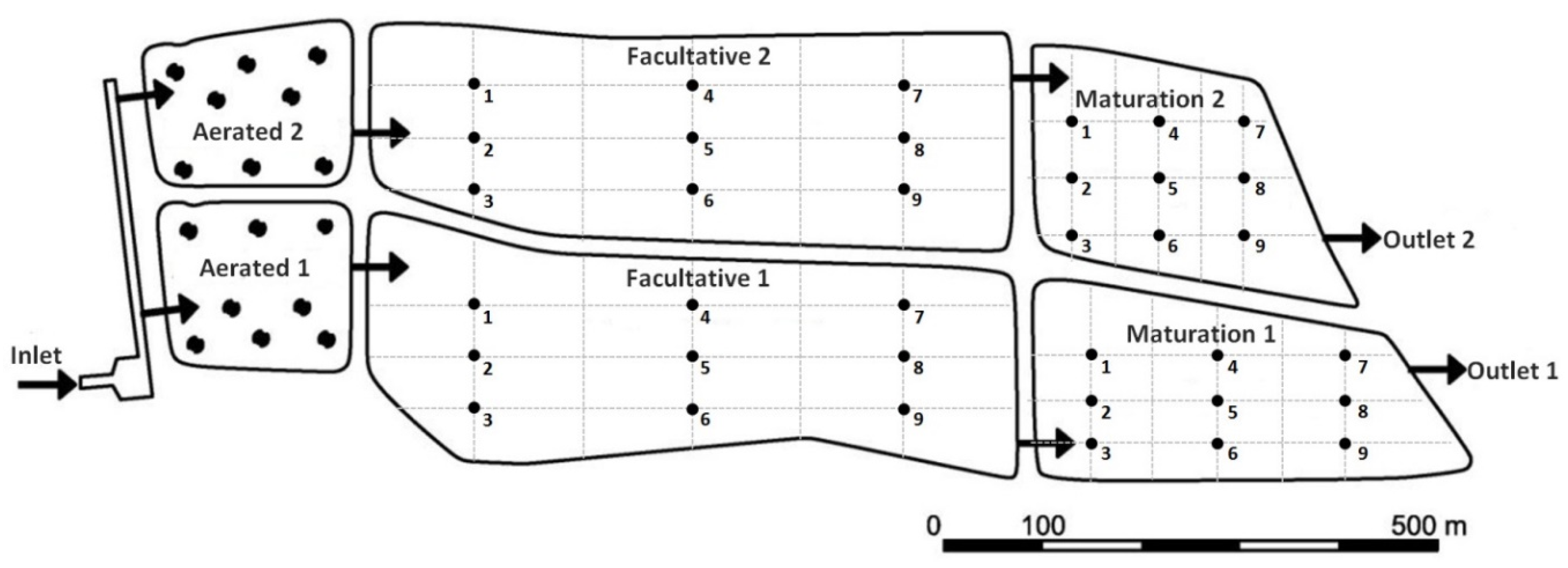
2.1. Study Area

The Ucubamba WSP is located at 2°52′21″ S, 78°56′30′ W, at an altitude of 2400 m above sea level and is designed to treat the domestic effluent from the city of Cuenca (Ecuador). The annual average temperature is 14 °C. The dry season is between June and December, and the rainy season is between January and May. The total surface of the WSP is 45 ha and the hydraulic retention time (HRT) is 11.5 days [21]. The WSP is in operation since 1999 by the Municipal Company ETAPA (Empresa Municipal de Telecomunicaciones, Agua Potable, Alcantarillado y Saneamiento) in Cuenca, Ecuador. Wastewater entering the WSP first passes through a pre-treatment step (screening and grit chamber). After this primary treatment, the wastewater is divided into two identical flow lines (Figure 1). Wastewater flows into an aerated lagoon, which contains mechanical floating aerators to provide oxygen for the removal of organic matter. The HRT is relatively short (i.e., two to three days). The total area of the aerated lagoons is 6 ha, with a depth of 4.5 m (two times 3 ha). Subsequently, the aerated wastewater flows from the aerated lagoon into the FPs, where further removal of soluble BOD takes place. The total area of the FPs is 26 ha, with a depth of 2 m (two times 13 ha) and the theoretical HRT is five to six days. The MPs are the last stage in the biological treatment chain and mainly remove pathogens [22]. The total area of the MPs is 13 ha with a depth of 1.8 m (7.4 ha in MPs from line 1 and 5.6 ha in line 2) and the HRT is three to four days. With no inclination, the bottom of the ponds is well-sealed by geotextiles to avoid seepage.

2.2. Sampling Scheme

In order to have representative samples for the whole pond, each pond was divided into 6 sections longitudinally and 4 sections transversally. Sampling was done at nine different locations (S1–S9) across the FPs and MPs, to measure the physical, chemical and biological characteristics (Figure 1). At each location, a multi-probe YSI 6600V2-2 (YSI Xylem Inc., Yellow Springs, Ohio, USA) was used to measure DO, chlorophyll a and water temperature at two depths, i.e., 30 cm below the water surface and 15 cm above the sediment layer of the ponds. Due to sludge accumulation at locations 1 and 2 of the FPs, only samples at 30 cm below the water surface were collected for these two locations. At the same time, a sampling device (Teledyne ISCO, model 6712, Teledyne Isco Inc, Wierde, Belgium) was used to collect the water samples at different locations and depths; three samples from the locations at a similar distance from the inlet (e.g., locations 1, 2 and 3) were mixed as one sample, resulting in 3 mixed samples per pond and per depth. These mixed samples were sent to the lab in ETAPA for biochemical oxygen demand (BOD) analysis using American Public Health Association methods (code 5210) [23]. Three sampling campaigns were implemented on 25 and 26 July (T1), 14 and 15 August (T2) and 26 and 27 August (T3) in 2013. At each sampling time, one WSP line was sampled over the course of one day, starting from 8:00 to 17:00. Average air temperature, solar radiation and wind speed were obtained from the Meteorological Station of CELEC Hidropaute, located approximately 600 m away from the WSP.

2.3. Model Construction and Diagnostics

2.3.1. Variables Used to Develop Models

GLMs were applied to predict the DO levels of both FPs and MPs. The Statistical Package for the Social Sciences (SPSS) version 22 by IBM was used for model construction and the coefficients of the variables were obtained by backward regression method [24]. The approach begins by including all predictors in the model and then calculating the contribution of each one by looking at the significance value of the t-test, which was used to test whether the coefficient was different from 0, for each predictor. This significance value was compared against a removal criterion (which could be either an absolute value of the test statistic or a probability value for that test statistic). If a predictor met the removal criterion (i.e., if it did not make a statistically significant contribution to how well the model predicted the outcome variable) it was removed from the model and the model was re-estimated including only the remaining predictors. The contribution of the remaining predictors was then reassessed in a similar fashion, until only significant predictors were left in the model. In this study, the default stepping method criterion in SPSS was used for variable selection. Variables could be entered or removed from the model, depending on the significance (probability) values in the t-test. A variable was entered into the model, if the significance value of its t-test was less than 0.05 (Entry value) and was removed if the significance level was greater than 0.1 (Removal value).

Six variables, i.e., chlorophyll a, BOD, water temperature, solar radiation, wind speed and air temperature, were always used as predictors in the models, given the mass balance of oxygen in the ponds. While the main oxygen sources in the WSP system were photosynthesis and the direct exchange of atmospheric oxygen through the air/water interface, oxygen consumption was mostly done by aerobic bacteria for mineralizing organic matter and nitrification process [25]. Additionally these six variables, depths ranging from 5 to 175 cm from the water surface, and timing (the time-points when the samples were taken) ranging from 8:00 to 17:00, were used in some of the models to test whether this inclusion would result in better model performance. The general predictive model of the DO was showed as follows:

$$\mathrm{DO}={\mathsf{\beta }}_0+{\mathsf{\beta }}_1\times \mathrm{Chl}+{\mathsf{\beta }}_2{\times \mathrm{BOD}}_5+{\mathsf{\beta }}_3\times \mathrm{WT}+{\mathsf{\beta }}_4\times \mathrm{SR}+{\mathsf{\beta }}_5{\times \mathrm{WS}+\mathsf{\beta }}_6\times \mathrm{AT}+{\mathsf{\beta }}_7{\times \mathrm{Depth}+\mathsf{\beta }}_8\times \mathrm{Timing}$$

(1)

where Chl: Chlorophyll a; BOD: Biological oxygen demand; WT: Water temperature; SR: Solar radiation; WS: Wind speed; and AT: Air temperature;

2.3.2. Model Development

Different data partitioning strategies were made to develop predictive models of DO. These strategies took into account the potential effects of sampling campaigns (T1, T2 and T3), depth (surface and bottom), pond types (FP and MP), pond lines (lines 1 and 2), ponds (FP1, FP2, MP1 and MP2) and sampling timing (morning and afternoon) (Figure 2). The data partitioning generated seven types of datasets—(1) a complete dataset; (2) three campaign-specific datasets; (3) three depth-specific datasets; (4) six depth-and-pond-type-specific datasets; (5) four depth-and-pond-line-specific datasets; (6) eight depth-and-pond-specific datasets; and (7) eight depth-and-pond-specific datasets, taking into account the Timing factor. From these datasets, two-third of the datasets were used for training the models and one-third of the datasets were used for validating the trained models. From the combination of the data partition and cross validation, 83 models were produced in total. Details of the 83 models can be found in Supplementary Material S1.

2.3.3. Model Diagnostics and Assessment

The presence of outliers in the dataset was detected and checked by a number of measures provided in SPSS, such as Cook’s distance, standardised residuals, average leverage, Mahalanobis distance, standardised DFBeta (in SPSS, DFBeta is defined as the difference between a parameter estimated using all cases and that estimated when one case is excluded) and Covariance ratio (CVR). Additionally, assumptions of GLMs were also taken into account, following the guidelines of Zuur, et al. [26]. Major assumptions of GLMs are—(1) homoscedasticity, which could be checked by the plot of the standardised residuals and the standardised predicted values; (2) independent errors, which could be checked by a Durbin–Watson test. As generally accepted, the Durbin–Watson value should be in the range of 1–3, and the closer to 2, the better; (3) multicollinearity, which could be determined by a variance inflation factor (VIF) > 10 and (4). Normally distributed errors, which could be observed by histogram of the standardised residuals and the normal probability plot of standardised residuals. For prediction purpose, it is not necessary to meet all assumptions, especially in ecological data, where the assumptions are difficult to meet and, therefore, evaluation of the models preferably focuses on the validity of the predictions in the new data. However, better predictions would result from a model that satisfied its underlying assumptions.

2.4. Model Comparison

In this study, two measures were used to compare the predictive accuracy of the models. They were the mean absolute error (MAE), showing how different the predicted value was from the observed value, and the symmetric mean absolute percentage error (SMAPE), showing the difference of the predicted and the observed value in percentage. MAE is a common measure of predictive accuracy [27] and is defined as the average sum of the absolute difference between the observed and the predicted values, while SMAPEs exist in several versions. Since predicted DO could be negative and the DO values especially near the bottom could be close to 0, SMAPEs formula introduced by [28] was used in this study and was modified to have the range from 0 to 100%. The MAE and SMAPE obtained during the validation of models constructed for different types of datasets were compared with each other and the optimal models were those that had the smallest MAE and the smallest SMAPE. The formulas to calculate MAE and SMAPE were as follows:

$$\mathrm{MAE}=\frac{1}{\mathrm{n}}{\displaystyle \sum }_{\mathrm{i}=1}^{\mathrm{n}}\left|{\mathrm{O}}_{\mathrm{i}}-{\mathrm{F}}_{\mathrm{i}}\right|$$

(2)

$$\mathrm{SMAPE}(\%)=\left[\frac{1}{\mathrm{n}}{\displaystyle \sum }_{\mathrm{i}=1}^{\mathrm{n}}\frac{\left|{\mathrm{O}}_{\mathrm{i}}-{\mathrm{F}}_{\mathrm{i}}\right|}{\left(\left|{\mathrm{O}}_{\mathrm{i}}\right|+\left|{\mathrm{F}}_{\mathrm{i}}\right|\right)}\right]\times 100\%$$

(3)

where O_i is the observed value and F_i is the predicted value and n is the number of data points.

2.5. Model Parameters and Their Importance

The coefficients of the models are important parameters, as they give information about the relationship between the outcome variable and each predictor variable. If the coefficient was positive, there was a positive relationship between the predictor variable and the outcome variable, while a negative coefficient represent a negative relationship [29]. Moreover, the coefficients also provide information about to what degree each predictor variable affects the outcome variable, if effects of all other predictor variables were held constant. Due to the difference in units of measurement of the predictor variables, standardised coefficients were preferably used to interpret the importance of each predictor variable [30]. The standardised coefficients represent the number of standard deviations that the outcome would change, as a result of one standard deviation change in the predictor. The standardised beta values were all measured in standard deviation units and so were directly comparable, therefore, they provided a better insight into the ‘importance’ of a predictor variable in the model. The degree of importance of the predictor variable to the outcome variable can be known by comparing the absolute values of the standardised coefficients. The larger the absolute value of the standardised coefficient, the more important the predictor variable.

3. Results

3.1. Variability of Physicochemical and Biological Parameters and Climatic Conditions in the Ponds

The sampling campaign was done in three different sampling times (T1, T2 and T3) to collect the data for modelling dissolved oxygen (DO) in both FPs and MPs. The variability of physicochemical and biological parameters and climatic conditions are showed in Supplementary Material S2. The data of chlorophyll a differed highly between the sampling times and depths (surface vs. bottom), which could be related to the timing of sampling (morning or afternoon). Chlorophyll a concentration also differed between the two depths within the pond and between the two different ponds (FPs vs. MPs). In general, the concentration of chlorophyll a at the surface was higher than that at the bottom and the concentration of chlorophyll a in the FPs was higher than that in the MPs. Specifically, the algal biomass near the water surface was around double that at the bottom. This proportion was lower in the FPs (around 1.5) but higher in the MPs (around 2.5). Higher algal biomass could also be found in the FPs compared to their consecutive ponds, i.e., 354.8 and 161 µg Chl a L⁻¹_. The concentration of BOD followed more or less the same pattern as chlorophyll a, except that there was no large variability of BOD concentration between the three different sampling times, which could be appointed to the quite stable BOD removal efficiency of the system. It was also observed that the concentration of BOD decreased from the FPs to MPs by a factor of two, i.e., 33.7 and 18.8 mg L⁻¹. Water temperature did not change that much between the three sampling times, and fluctuated around 18–19 °C. Additionally, water temperature seemed to be homogenous throughout the water column and between the two pond types. Related to the climatic conditions, only air temperature remained unaltered, i.e., 16.8 ± 2.1 °C, while wind speed and especially solar radiation did change a lot across the three sampling times, i.e., 2.4 ± 1.0 m s⁻¹ and 469.2 ± 223.8 W m⁻², respectively. As DO was in fact influenced by the BOD concentration and the diurnal activity of algae, it also showed a large variability across the three sampling times (Figure 3). Between the two pond types, DO across the three sampling times had a larger variability in FPs than in MPs. There was also a difference of DO between the surface and bottom of both FPs and MPs. Within line 1 of the WSP, there was a decrease of DO from FP 1 to MP 1, in both the surface and the bottom, while in line 2 of the WSP, DO throughout the ponds were more or less the same in both the surface and the bottom layers. From the outlet part of FP1 to MP1 inlet, DO values near the water surface dropped about 70%, i.e., from above 10 mg O₂·L⁻¹ to around 3 mg O₂·L⁻¹, while the oxygen level remained similar between the two ponds in the upper line.

3.2. Optimal Models for Prediction of Dissolved Oxygen in the Ponds

In total, 83 different models were built from seven data partitioning and cross-validation strategies (Figure 2). The best-performing model(s) (the one with lowest MAEs and SMAPEs in both the training and validation periods) of each dataset was selected as the representative model(s) of that dataset and then compared to each other to find the optimal models for prediction of DO in the WSP (Figure 4 and Figure 5). The obtained results showed that the optimal models were the ones constructed separately for ponds and depths, as in general they had lowest MAEs and SMAPEs among the others. The details of all models constructed for all datasets can be found in Supplementary Material S3.

Related to predictive accuracy, it can be seen from

Table 1. Predictive accuracy of the optimal models.

Pond	Training Dataset	Validation Dataset	Full Optimal Model	MAE ± sd (mg L−1)		SMAPE ± sd (%)		R2
				Training	Validation	Training	Validation
FP1_Surface	T2T3 FP1_Surface	T1 FP1_Surface	DO = −43.718 + 0.039Chl + 0.204BOD + 1.772AT	1.59 ± 0.73	3.06 ± 2.74	11.75 ± 14.17	11.01 ± 10.03	0.909
FP1_Bottom	T2T3 FP1_Bottom	T1 FP1_Bottom	DO = −9.550 + 0.447BOD	2.75 ± 2.20	3.52 ± 3.00	38.70 ± 31.49	20.08 ± 24.08	0.540
MP1_Surface	T1T2 MP1_Surface	T3 MP1_Surface	DO = −2.024 + 0.012Chl + 0.007SR	0.54 ± 0.46	0.74 ± 0.43	17.50 ± 21.64	17.64 ± 10.07	0.854
MP1_Bottom	T1T2 MP1_Bottom	T3 MP1_Bottom	DO = 7.470 − 0.445WT + 0.095AT	0.22 ± 0.18	0.79 ± 0.46	30.61 ± 17.28	49.19 ± 30.84	0.391
FP2_Surface	T1T3 FP2_Surface	T2 FP2_Surface	DO = −40.463 + 0.014Chl + 0.201BOD + 1.448WT + 0.496AT	1.07 ± 0.67	3.54 ± 2.62	12.66 ± 9.47	20.91 ± 10.35	0.752
FP2_Bottom	T1T3 FP2_Bottom	T2 FP2_Bottom	DO = −2.494 + 0.119BOD	0.29 ± 0.22	1.19 ± 1.10	25.29 ± 13.71	51.89 ± 25.79	0.424
MP2_Surface	T1T2 MP2_Surface	T3 MP2_Surface	DO = −15.016 + 0.016Chl + 1.952WT+ 0.004SR − 0.947WS − 0.969AT	0.32 ± 0.27	1.14 ± 0.77	2.35 ± 2.00	10.88 ± 6.42	0.885
MP2_Bottom	T1T2 MP2_Bottom	T3 MP2_Bottom	DO = −5.773 + 0.018Chl + 0.407BOD	0.55 ± 0.32	1.30 ± 1.35	13.51 ± 12.82	71.62 ± 33.56	0.624

FP = Facultative pond; MP = Maturation pond; DO = Dissolved oxygen; Chl = Chlorophyll a; BOD = Biological oxygen demand; WT = Water temperature; SR = Solar radiation; WS = Wind speed; AT = Air temperature; MAE = Mean absolute error; SMAPE = Symmetric mean absolute percentage error and sd = Standard deviation.

that MAE varied in the range of 0.22–2.75 mg L⁻¹ in the training period and 0.74–3.54 mg L⁻¹ in the validation period. To express the predictive accuracy in percentage, SMAPEs were also calculated and it was in the range of 2.35–38.70% in the training period and 10.88–71.62% in the validation period. In general, among the ponds, the model of MPs performed better than those of FPs, and within a pond, the models for the surface performed better than those for the bottom. This was supported by the higher MAEs and SMAPEs values in the optimal models of FPs, compared to those of MPs, and in the optimal models for the bottom compared to those for the surface (Table 1).

3.3. Importance of the Predictor Variables

In GLMs, standardised coefficients are used to determine the degree of importance of each predictor variable to the outcome variable [29]. They are also used to determine to what degree each predictor variable affects the outcome variable, if all other predictor variables are kept constant. The overview of the parameters of the optimal models and their important statistics are shown in

Table 2. Model parameters and the importance of the predictor variables.

Model	Model Parameter	Mean	Standard Deviation	Unstandardised Coefficient		Standardised Coefficient	95% Confidence Interval for Coefficient		Change of DO by Change of Each Variable †
				Coefficient	Standard Error		Lower Bound	Upper Bound
FP1 Surface	DO	11.28	5.90
	Constant			−43.718	5.975		−56.533	−30.904
	Chlorophyll a	430.22	109.10	0.039	0.005	0.713*	0.028	0.049	4.21
	BOD	41.67	7.74	0.204	0.068	0.268*	0.058	0.351	1.58
	Air temperature	16.87	2.09	1.772	0.238	0.626*	1.263	2.282	3.69
FP1 Bottom	DO	5.17	5.31
	Constant			−9.550	4.050		−18.375	−0.725
	BOD	32.93	8.72	0.447	0.119	0.735*	0.187	0.707	3.90
MP1 Surface	DO	2.46	1.89
	Constant			−2.024	0.511		−3.113	−0.935
	Chlorophyll a	245.73	108.63	0.012	0.002	0.678*	0.008	0.016	1.28
	Solar radiation	228.86	121.67	0.007	0.002	0.448*	0.004	0.010	0.85
MP1 Bottom	DO	0.402	0.369
	Constant			7.470	2.299		2.571	12.370
	Water temperature	18.59	0.86	−0.445	0.143	−1.035*	−0.750	−0.139	−0.38
	Air temperature	12.60	3.25	0.095	0.038	0.833*	0.014	0.176	0.31
FP2 Surface	DO	4.92	2.58
	Constant			−40.463	10.646		−63.462	−17.463
	Chlorophyll a	343.74	128.96	0.014	0.003	0.691*	0.006	0.021	1.78
	BOD	31.67	6.87	0.201	0.061	0.536*	0.070	0.333	1.38
	Water temperature	18.21	0.66	1.448	0.659	0.371*	0.025	2.871	0.96
	Air temperature	15.88	2.06	0.496	0.216	0.396*	0.029	0.962	1.02
FP2 Bottom	DO	0.60	0.49
	Constant			−2.494	1.046		−4.773	−0.215
	BOD	25.93	2.70	0.119	0.040	0.651*	0.032	0.207	0.32
MP2 Surface	DO	6.87	1.14
	Constant			−15.016	12.656		−42.590	12.558
	Chlorophyll a	242.92	63.72	0.016	0.002	0.910*	0.011	0.021	1.04
	Water temperature	19.32	0.23	1.952	0.688	0.387*	0.453	3.451	0.44
	Solar radiation	568.57	193.24	0.004	0.001	0.604*	0.001	0.006	0.69
	Wind speed	3.73	1.05	−0.947	0.174	−0.871*	−1.326	−0.558	−0.99
	Air temperature	18.89	0.46	−0.969	0.376	−0.386*	−1.787	−0.151	−0.44
MP2 Bottom	DO	2.51	1.05
	Constant			−5.773	1.723		−9.446	−2.100
	Chlorophyll a	67.04	33.85	0.018	0.006	0.592*	0.005	0.032	0.62
	BOD	17.33	2.63	0.407	0.082	1.016*	0.233	0.581	1.07

Note: * p < 0.05; † the change of DO (mg L⁻¹) when there was a change of one standard deviation of a variable while the effects of all other variables were kept constant.

. It can be seen from the values of the standardised coefficients that chlorophyll a was the most important predictor variable in all models for the surface of the ponds, while in the models for the bottom, BOD was the most important variable to DO, except for the model of MP1. Particularly, in the model of FP1 at the surface chlorophyll a, BOD and air temperature made a significant contribution to the prediction of DO. They all had a positive relationship with DO, indicating that an increase of each variable will result in an increase of DO. Among the three predictor variables, chlorophyll a was the most important one as it had the highest standardised coefficient (0.713), while air temperature was the second important one (0.626) and BOD was the third important one (0.268). The values of the standardised coefficients also indicated that as chlorophyll a increased by one standard deviation (109.10 µg L⁻¹), DO increased by 0.713 standard deviation, which was equal to 0.713 × 5.90 = 4.21 mg L⁻¹ (Table 2). Similarly, an increase of one standard deviation of air temperature (2.09 °C) and BOD (7.74 mg L⁻¹) would result in an increase of 3.69 (0.626 × 5.90) and 1.58 (0.268 × 5.90) mg L⁻¹ DO, respectively. Similar interpretations could be made for the other models, based on the values of the standardised coefficients in the last column of Table 2.

4. Discussion

4.1. Variability of the Physicochemical and Biological Parameters and Climatic Conditions in the Ponds

As the timing of sampling differed for each location, it could affect the variability of variables such as chlorophyll a and climatic conditions, which made it difficult to compare the difference of variables between the three sampling times. This was supported by the data of line 2, which was always sampled in the morning and, therefore, varied less between the three sampling times. In general, DO and chlorophyll a showed a large difference and variability between the two depths, between the two pond types and across the three samplings. The variability of these two parameters reflected the temporal and spatial dynamics of the micro-algal photosynthesis taking place in the ponds, as the variability of climatic conditions across the sampling times was also observed. Although it had a higher organic loading, the average DO in FPs was higher than that in the MPs. This could be associated with the higher chlorophyll a in the FPs, resulting in higher photosynthesis. This finding was in line with what is normally observed in most WSPs [31]. According to Pearson [31], total algal biomass, as determined by the chlorophyll a concentration in FPs, is usually higher than that in the subsequent MPs of the same series. This probably reflects the reduction in the available nutrients, and the increased grazing pressures by the zooplankton population that occurs in the more aerobic conditions prevailing in MPs [32]. Additionally, there was a logical difference of chlorophyll a and DO concentration between the surface and bottom of the WSP. Although repeated samplings were not done at the same times of the day, the average concentration of chlorophyll a and DO near the surface were always higher than that near the bottom. This could be associated with the photosynthesis of microalgae that occurred stronger at the surface of the ponds because of the sunlight [33]. However, it was also interesting to note that the maximum concentration observed in the WSP was 500 µg L⁻¹, which was considered to be low, according to Mara [1], as the chlorophyll a concentration in “healthy” WSPs is usually in the range of 500–2000 μg L⁻¹. Therefore, more samplings and long-term data collection should be done to figure out whether this low concentration of chlorophyll a was related to short-term data collection, or this could be a characteristic of a WSP operating at a high altitude [34,35,36,37,38].

BOD in the WSP did not show a large variability between the surface and the bottom, within a pond and across the three sampling times. First, this could be related to the use of mixed samples of BOD, resulting in less variability of BOD values between different locations. Second, it should be noted that the BOD samples were unfiltered BOD, causing the presence of algae in the samples to interfere with BOD values. The latter could be the case in this study, as it was reported by Gerardi [39] that in the BOD test, algae consumed DO to break down the substrate. When they die in the BOD bottle, they become substrate for heterotrophic bacteria in the BOD bottle that respire using DO. Consequently, these processes inflate the value of the BOD test in WSPs. Therefore, in order to determine the real BOD value, algae must be filtered from the sample tested for BOD.

The WSP in this study was situated at an altitude of 2400 m above sea level, in the Sierra of the Andes, the southern region of Ecuador, featuring a subtropical highland climate. The average daily temperature was relatively constant throughout the year. Consequently, there was no large difference on the average temperature between the dry and wet seasons. However, the daily fluctuations in temperature over 24-h periods are much more pronounced, meaning that temperature stratification can occur during daytime [38,40]. However, this was not the case in this study as no large difference and variability of water temperature between the surface and the bottom was observed in the ponds. This result implied that mixing (at least during the sampling period) occurred inside the system, which could be related to the wind and the hydraulic conditions of the ponds.

4.2. Model Comparison

The 8 optimal models (Table 1) selected for prediction of DO were the best-performing ones among the 83 models that were evaluated based on predictive accuracy (MAEs and SMAPEs). These optimal models were obtained as follows. First, different models developed from one type of dataset were compared to each other regarding their predictive performance, based on MAEs and SMAPEs, in both the training and validation periods. Second, the optimal model(s) of different dataset types were compared to each other, based on the same criteria, to obtain the optimal models.

In general, the optimal models of pond-and-depth-specific datasets had lower predictive accuracy compared to the optimal models of a complete dataset and depth-and-pond-type-specific datasets. Related to the optimal models of pond-and-depth-specific datasets with the Timing factor, it should be noted that these models were the same optimal models of pond-and-depth-specific datasets, without including Timing. When the factor was included, it resulted in only a small increase of the predictive performance of the model. For example, in the case of the model for DO at the surface of MP2, MAEs decreased from 0.32 and 1.14 to 0.29 and 0.99 mg L⁻¹ in the training and validation periods, respectively, and the SMAPEs decreased from 2.35 % and 10.88 % to 2.10 % and 9.46 % in the training and validation periods, respectively. Since DO dynamics in the ponds follow diurnal circles [20], timing was expected to have a strong effect on model predictive performance, this was not the case in this study.

4.3. Predictive Accuracy of the Optimal Models

MAE is one of the most commonly reported measures of predictive accuracy [41]. In this study, it was used to compare the predictive accuracy, which is the difference between the observed and predicted values of DO in the constructed models. Since this measure did not give the predictive accuracy in percentage, it is possible that a model with a small MAE could have a high SMAPE [28]. Therefore, SMAPEs were used alongside MAEs in selecting the optimal models. Additionally, predictive accuracy (MAEs and SMAPEs) was evaluated in both the training and validation periods, to increase the reliability of the selected optimal models, following the bias-variance trade-off principle [42]. It was shown, based on the measures of predictive accuracy, that the models of MPs performed better than those of FPs. This could be associated with the fact that FPs stabilise the incoming wastewater with varying BOD concentrations from the aerated ponds, resulting in high variability of many related parameters and creating a more dynamic and turbulent environment inside these ponds. Moreover, as FPs receive a higher organic loading than MPs, this would create a more dynamic algal community than the one in MPs [40,43]. As a result, oxygen produced by algae in FPs becomes more dynamic (variability) than in MPs, which in turn affected the models being trained. This was supported by the MAEs and SMAPEs showed in Table 2, where the MAEs of DO in the MPs (0.22–0.55 mg L⁻¹ and 0.74–1.30 mg L⁻¹ in the training and validation periods, respectively) was lower than that in the FPs (0.29–2.75 mg L⁻¹ and 1.19–3.54 mg L⁻¹ in the training and validation periods, respectively). Similarly, SMAPEs of MPs (2.35–30.61% and 10.88–71.62% in the training and validation periods, respectively) were also lower than those of FPs (11.75–38.70% and 11.01–51.89% in the training and validation periods, respectively).

4.4. Importance of the Predictor Variables in the Optimal Models

As seen in Table 2, chlorophyll a was the most important predictor variable of the models for the surface of the ponds, indicating that algae played an important role in driving DO at the surface of the WSPs. This result was in line with the literature, where it was reported that most oxygen production takes place at the surface of WSPs [44]. This result was useful for the pond manager to steer DO in the ponds, as to obtain a high concentration of DO at the surface of the WSPs, the pond manager should focus on the maintenance of a healthy algal biomass in the ponds, so that it can provide sufficient DO for organic matter oxidation through heterotrophic bacteria and minimise ecological impacts when pond the effluent is discharged into the water bodies [16]. Related to the models for the bottom of the ponds, BOD was the most important predictor in 3 out of 4 models, indicating the effect of BOD on the bottom DO.

Although chlorophyll a and the BOD variables were present in most of the optimal models, their coefficients were lower than other variables in the same optimal model, which could imply that they might not be the most influential variables on the output of DO. However, their presence in the models revealed that they were good representative predictors for the prediction of DO in the ponds, reflecting the influence of photosynthesis and organic loading. However, DO dynamics in the ponds were also affected by other physicochemical parameters, such as water temperature and climatic conditions. Therefore, these variables were also included in the optimal models with high coefficients, which indicate their strong effect on DO during the period that the data was collected. This finding again confirmed the high complexity of WSPs, as any process that occurs in the ponds is influenced/driven by a large number of physical, chemical, biological and environmental factors [45].

4.5. Application and Limitations of the Models

The GLMs developed in this study showed good prediction accuracy and reliable performance, which could be used as a useful tool to predict DO in the ponds. They also provided primary insights into important variables driving DO in the ponds. However, it should be noted that the coefficients of BOD were positive in all optimal models. The reason for this could be due to the presence of algae in the samples, which was believed to interfere with the results of the BOD analysis [39]. This could narrow the range of the BOD values and, therefore, might affect the coefficients of BOD. Another reason could be associated with short-term sampling data, which might not capture the whole variability of the physicochemical and biological parameters of the WSP.

It is important to collect enough data to obtain reliable GLMs [46]. However, due to resource and time constraints, only a limited number of short-term data was collected to develop and validate the models. This might limit the reliable application of models in predicting DO year-round, and affects the predictive power of GLMs in general. As seen in Table 2, the optimal models of both FPs and MPs predicted DO precisely in the training period. However, when they were used to predict a new dataset (validation), there was a small drop in their predictive power, implying that the optimal models were not generalised well and still needed to be further improved. More data should be collected to develop more reliable models before other causal reason(s), such as modelling techniques and methods, are addressed.

Many regression techniques are available for the development of predictive models and the application of different techniques would lead to different optimal models. In this study, backward regression was chosen, as it is a widely used method for developing GLMs, for prediction purpose [46]. Since the backward selection method relies on the algorithm-selecting variables, based on mathematical criteria, many authors argue that this takes many important methodological decisions out of the hands of the researcher [47]. The models derived by the algorithm often take advantage of sampling variability or sampling error, which is implied when the statistical characteristics of a population are estimated from a subset or sample of that population, and so decisions about which variables should be included are based on slight differences in their semi-partial correlation [48]. However, these slight statistical differences might contrast dramatically with the theoretical importance of a predictor to the model. There was also a danger of over-fitting (having too many variables in the model that essentially made little contribution to predicting the outcome) and under-fitting (leaving out important predictors) of the model [49]. Due to these disadvantages, a number of data points, which were not used in training models, were used to validate the models and the predictive accuracy of the models was evaluated in both the training and validation periods, so that the predictive power of the optimal model was maximised.

One of the largest limitations of GLMs applied in ecological data is the assumptions it has to meet [50]. Violation of GLMs assumptions is one of the reasons that makes model generalisation difficult. However, as the constructed models are used for prediction purpose, violation of these assumptions was considered to be less important, since the performances of the models were already evaluated based on their predictive accuracy (MAEs and SMAPEs). Moreover, due to the nature of the ecological data, which normally has a high variability between the data points, meeting all assumptions of GLMs is difficult to obtain in practice. However, it should be noted that when the assumptions of GLMs are met, the model could be accurately applied to the population of interest.

5. Conclusions

Three different sampling times were considered to collect physical–chemical and biological parameters, and the climatic conditions for the development of the predictive model of DO in a WSP in Cuenca, Ecuador. The results of this study showed that:

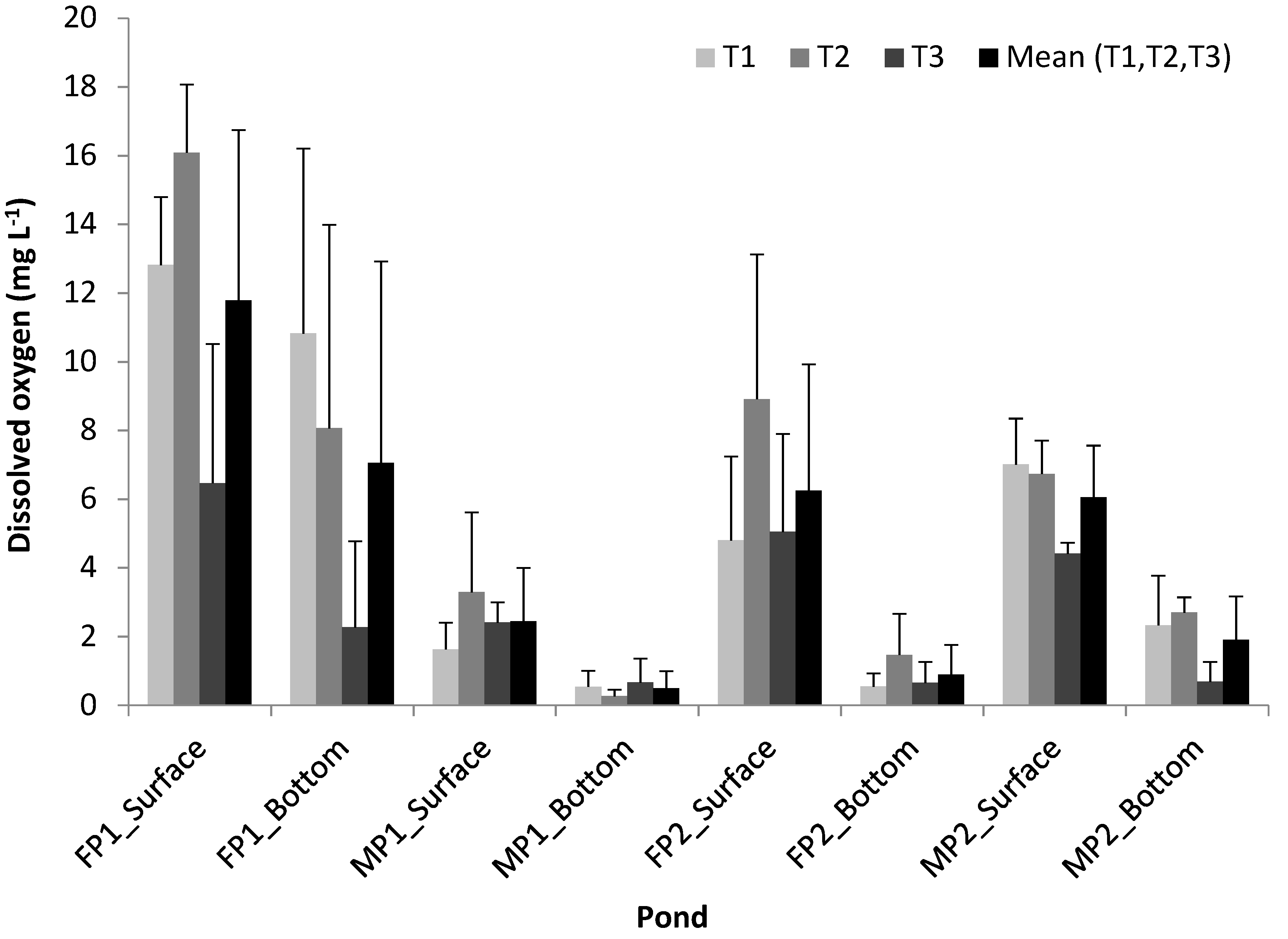
• There was a large variability of chlorophyll a, DO, and climatic conditions across the three sampling times. Within a pond, higher concentration of chlorophyll a and DO were observed near the surface than near the bottom. Between the two pond types, chlorophyll a and DO in the FPs were higher than those in the MPs. No large variability of BOD within a pond was observed across the three sampling times but there was a decrease of BOD from FPs to MPs.
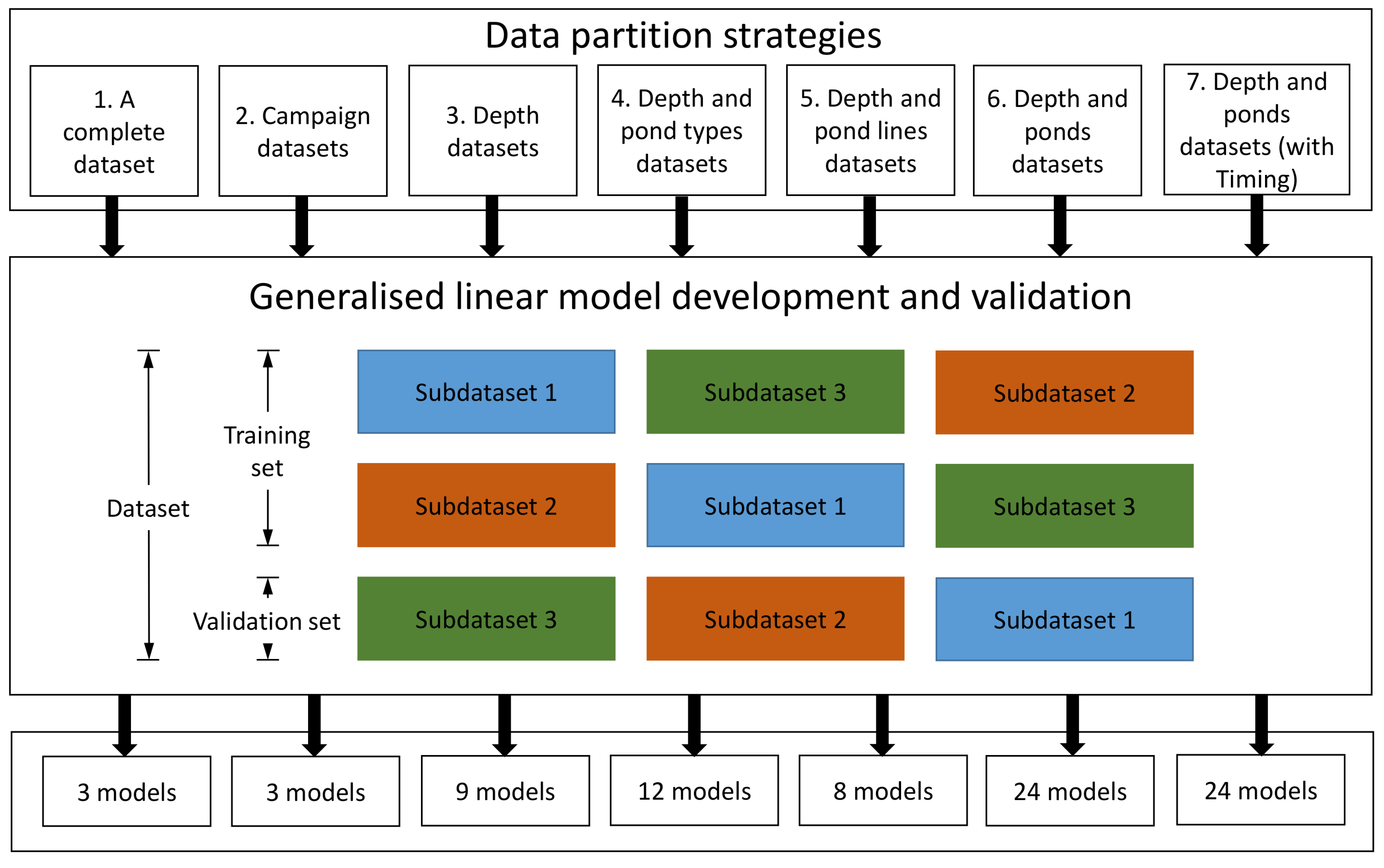
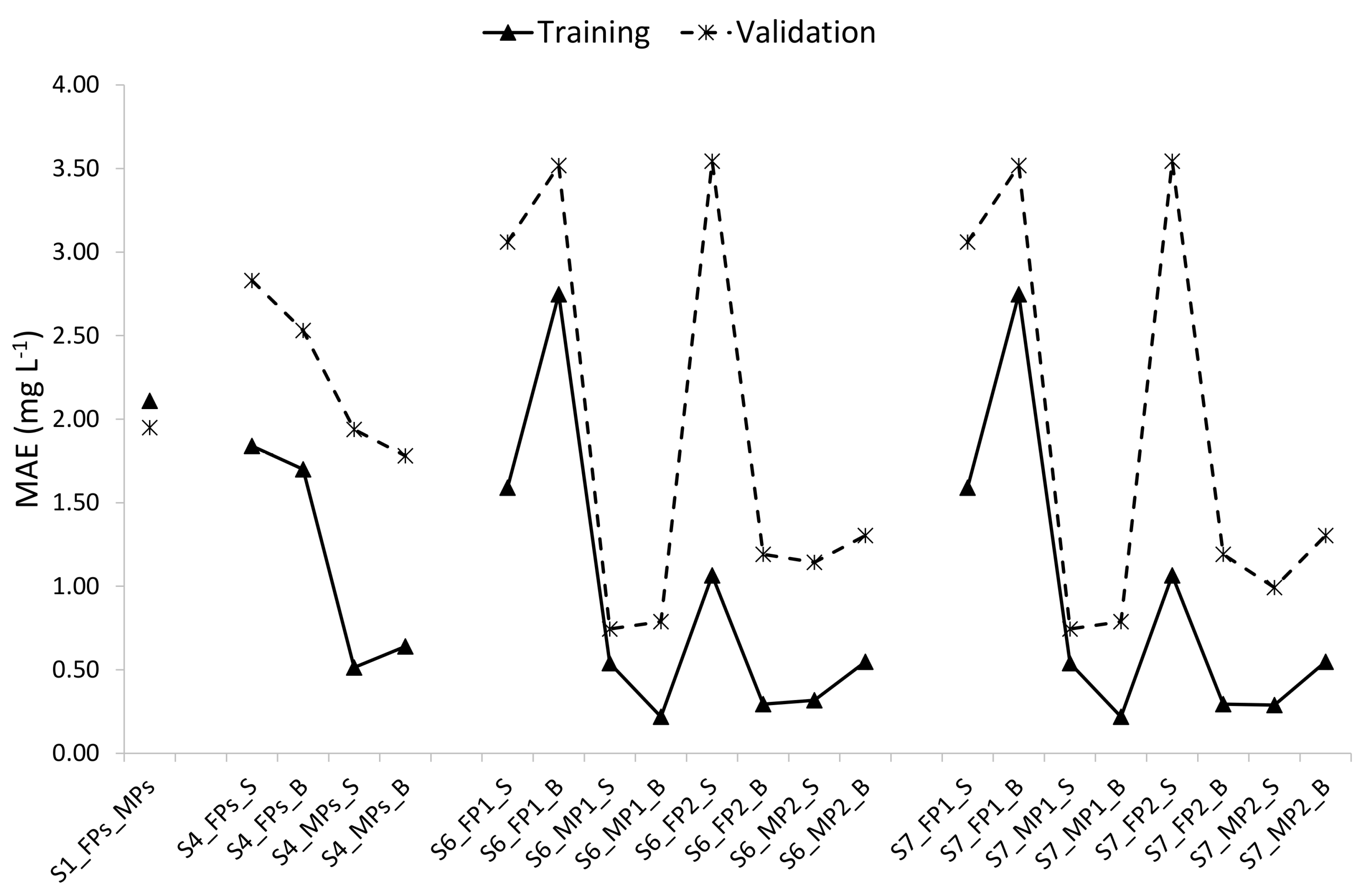
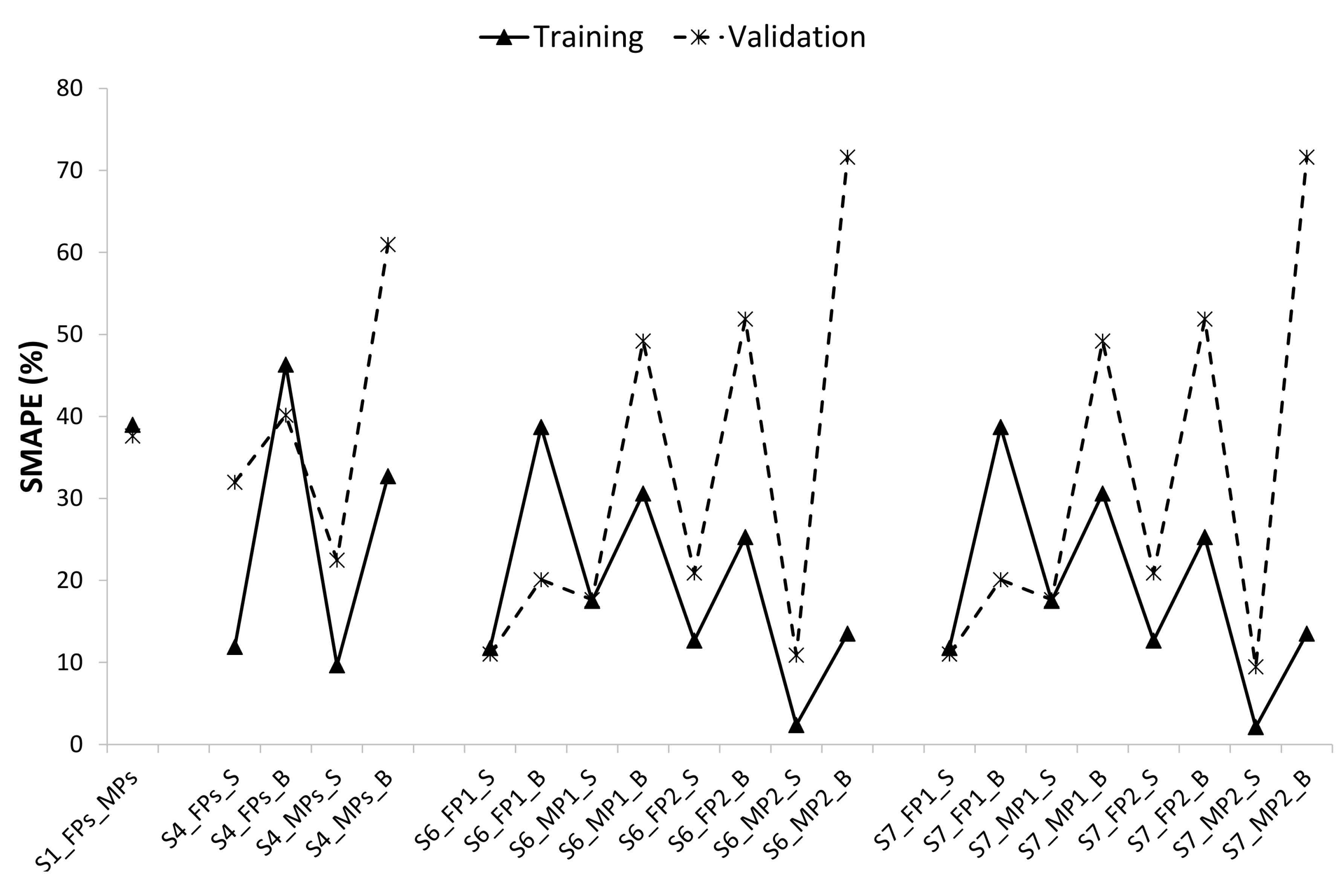
• Among the 83 models developed based on different data partitioning and cross-validation strategies, the 8 models developed specifically for each pond and each depth were the optimal ones. These optimal models depict varying MAEs of DO in the range of 0.21–2.75 mg L⁻¹, in the training period and 0.54–3.54 mg L⁻¹ in the validation period, and SMAPEs of dissolved oxygen were in the range of 3.18–38.70% in the training period and 7.54–89.24% in the validation period. Among the 8 optimal models, the optimal models of MPs performed better than those of FPs and within a pond, the optimal models for the surface seemed to perform better than those for the bottom.
• Among the variables used to predict dissolved oxygen, chlorophyll a and BOD appeared to be representative predictor variables. Additionally, water temperature and climatic conditions also highly influenced DO.
• The effect of the timing variable (expressed at the time points the samples were taken) did not show a strong effect on the prediction of DO.
• The results of this study are valuable in the management of WSP and provide basic insights into oxygen-related processes, which could help in further development of advanced models for WSPs.
• Despite the limitation of the data-driven approach for global extrapolation, it is expected that the data partitioning and cross-validation strategies developed in this study, could be widely applied to identify the optimal models for prediction purposes.

References

1. Mara, D.D. Domestic Wastewater Treatment in Developing Countries; Earthscan Publications: London, UK, 2004. [Google Scholar]
2. Ho, L.; Goethals, P.L.M. Municipal wastewater treatment with pond technology: Historical review and future outlook. Ecol. Eng. 2020, 148, 105791. [Google Scholar] [CrossRef]
3. Ho, L.T.; Van Echelpoel, W.; Goethals, P.L.M. Design of waste stabilization pond systems: A review. Water Res. 2017, 123, 236–248. [Google Scholar] [CrossRef]
4. Ho, L.; Goethals, P. Research hotspots and current challenges of lakes and reservoirs: A bibliometric analysis. Scientometrics 2020. [Google Scholar] [CrossRef] [Green Version]
5. Motulsky, H.; Christopoulos, A. Fitting Models to Biological Data Using Linear and Nonlinear Regression: A Practical Guide to Curve Fitting; Oxford University Press: Oxford, UK, 2004. [Google Scholar]
6. Hastie, T.; Tibshirani, R.; Friedman, J. The Elements of Statistical Learning: Data Mining, Inference, and Prediction; Springer: New York, NY, USA, 2013. [Google Scholar]
7. McDonald, J.H. Handbook of Biological Statistics; Sparky House Publishing, University of Delaware: Newark, DE, USA, 2009. [Google Scholar]
8. Sah, L.; Rousseau, D.P.; Hooijmans, C.M. Numerical modelling of waste stabilization ponds: Where do we stand? Water Air Soil Pollut. 2012, 223, 3155–3171. [Google Scholar] [CrossRef]
9. Wood, M.G.; Greenfield, P.F.; Howes, T.; Johns, M.R.; Keller, J. Computational fluid dynamic modelling of wastewater ponds to improve design. Water Sci. Technol. 1995, 31, 111–118. [Google Scholar] [CrossRef]
10. Shilton, A.; Mara, D.D. CFD (computational fluid dynamics) modelling of baffles for optimizing tropical waste stabilization pond systems. Water Sci. Technol. 2005, 51, 103–106. [Google Scholar] [CrossRef]
11. Alvarado, A.; Vesvikar, M.; Cisneros, J.F.; Maere, T.; Goethals, P.; Nopens, I. CFD study to determine the optimal configuration of aerators in a full-scale waste stabilization pond. Water Res. 2013, 47, 4528–4537. [Google Scholar] [CrossRef]
12. Dochain, D.; Gregoire, S.; Pauss, A.; Schaegger, M. Dynamical modelling of a waste stabilisation pond. Bioproc. Biosyst. Eng. 2003, 26, 19–26. [Google Scholar] [CrossRef]
13. Kayombo, S.; Mbwette, T.S.A.; Mayo, A.W.; Katima, J.H.Y.; Jorgensen, S.E. Modelling diurnal variation of dissolved oxygen in waste stabilization ponds. Ecol. Model. 2000, 127, 21–31. [Google Scholar] [CrossRef]
14. Ho, L.T.; Alvarado, A.; Larriva, J.; Pompeu, C.; Goethals, P. An integrated mechanistic modeling of a facultative pond: Parameter estimation and uncertainty analysis. Water Res. 2019, 151, 170–182. [Google Scholar] [CrossRef]
15. Ho, L.; Pompeu, C.; Van Echelpoel, W.; Thas, O.; Goethals, P. Model-based analysis of increased loads on the performance of activated sludge and waste stabilization ponds. Water 2018, 10, 1410. [Google Scholar] [CrossRef] [Green Version]
16. Sah, L.; Rousseau, D.P.L.; Hooijmans, C.M.; Lens, P.N.L. 3D model for a secondary facultative pond. Ecol. Model. 2011, 222, 1592–1603. [Google Scholar] [CrossRef]
17. Munoz, R.; Kollner, C.; Guieysse, B.; Mattiasson, B. Photosynthetically oxygenated salicylate biodegradation in a continuous stirred tank photobioreactor. Biotechnol. Bioeng. 2004, 87, 797–803. [Google Scholar] [CrossRef] [PubMed]
18. Mara, D.D.; Pearson, H.W. Waste Stabilization Ponds: Design Manual for Mediterranean Europe; World Health Organization. Regional Office for Europe: Geneva, Switzerland, 1998. [Google Scholar]
19. Pearson, H.W.; Mara, D.D.; Mills, S.W.; Smallman, D.J. Factors determining algal populations in waste stabilization ponds and the influence of algae on pond performance. Water Sci. Technol. 1987, 19, 131–140. [Google Scholar] [CrossRef]
20. Banks, C.J.; Koloskov, G.B.; Lock, A.C.; Heaven, S. A computer simulation of the oxygen balance in a cold climate winter storage WSP during the critical spring warm-up period. Water Sci. Technol. 2003, 48, 189–196. [Google Scholar] [CrossRef] [Green Version]
21. Alvarado, A.; Sanchez, E.; Durazno, G.; Vesvikar, M.; Nopens, I. CFD analysis of sludge accumulation and hydraulic performance of a waste stabilization pond. Water Sci. Technol. 2012, 66, 2370–2377. [Google Scholar] [CrossRef] [Green Version]
22. Verbyla, M.E.; Iriarte, M.M.; Guzman, A.M.; Coronado, O.; Almanza, M.; Mihelcic, J.R. Pathogens and fecal indicators in waste stabilization pond systems with direct reuse for irrigation: Fate and transport in water, soil and crops. Sci. Total Environ. 2016, 551, 429–437. [Google Scholar] [CrossRef] [Green Version]
23. APHA. Standard Methods for the Examination of Water and Wastewater; American Public Health Association (APHA): Washington, DC, USA, 2005. [Google Scholar]
24. SPSS Inc. SPSS-X User’s Guide; McGraw-Hill, Inc.: New York, USA, 1985. [Google Scholar]
25. Ellis, K.V. Stabilization ponds—Design and operation. Crit. Rev. Environ. Sci. Technol. 1983, 13, 69–102. [Google Scholar] [CrossRef]
26. Zuur, A.F.; Leno, E.N.; Elphick, C.S. A protocol for data exploration to avoid common statistical problems. Methods Ecol. Evol. 2010, 1, 3–14. [Google Scholar] [CrossRef]
27. Hyndman, R.J.; Koehler, A.B. Another look at measures of forecast accuracy. Int. J. Forecast. 2006, 22, 679–688. [Google Scholar] [CrossRef] [Green Version]
28. Goodwin, P.; Lawton, R. On the asymmetry of the symmetric MAPE. Int. J. Forecast. 1999, 15, 405–408. [Google Scholar] [CrossRef]
29. Rosner, B. Fundamentals of Biostatistics; Cengage Learning: Boston, MA, USA, 2010. [Google Scholar]
30. Zuur, A.F.; Ieno, E.N. A protocol for conducting and presenting results of regression-type analyses. Methods Ecol. Evol. 2016, 7, 636–645. [Google Scholar] [CrossRef]
31. Pearson, H. Microbiology of waste stabilization ponds. In Pond Treatment Technology; IWA publishing: London, UK, 2005; pp. 14–43. [Google Scholar]
32. Montemezzani, V.; Duggan, I.C.; Hogg, I.D.; Craggs, R.J. Control of zooplankton populations in a wastewater treatment High Rate Algal Pond using overnight CO2 asphyxiation. Algal Res. 2017, 26, 250–264. [Google Scholar] [CrossRef]
33. Ho, L.; Pham, D.; Van Echelpoel, W.; Muchene, L.; Shkedy, Z.; Alvarado, A.; Espinoza-Palacios, J.; Arevalo-Durazno, M.; Thas, O.; Goethals, P. A closer look on spatiotemporal variations of dissolved oxygen in waste stabilization ponds using mixed models. Water 2018, 10, 201. [Google Scholar] [CrossRef] [Green Version]
34. Pearson, H.W.; Mara, D.D.; Thompson, W.; Maber, S.P. Studies on high-altitude waste stabilization ponds in peru. Water Sci. Technol. 1987, 19, 349–353. [Google Scholar] [CrossRef]
35. Juanico, M.; Weinberg, H.; Soto, N. Process design of waste stabilization ponds at high altitude in Bolivia. Water Sci. Technol. 2000, 42, 307–313. [Google Scholar] [CrossRef]
36. Lloyd, B.J.; Leitner, A.R.; Vorkas, C.A.; Guganesharajah, R.K. Under-performance evaluation and rehabilitation strategy for waste stabilization ponds in Mexico. Water Sci. Technol. 2002, 48, 35–43. [Google Scholar] [CrossRef]
37. Recio-Garrido, D.; Kleiner, Y.; Colombo, A.; Tartakovsky, B. Dynamic model of a municipal wastewater stabilization pond in the arctic. Water Res. 2018, 144, 444–453. [Google Scholar] [CrossRef]
38. Ho, L.T.; Pham, D.T.; Van Echelpoel, W.; Alvarado, A.; Espinoza-Palacios, J.E.; Arevalo-Durazno, M.B.; Goethals, P.L.M. Exploring the influence of meteorological conditions on the performance of a waste stabilization pond at high altitude with structural equation modeling. Water Sci. Technol. 2018, 78, 37–48. [Google Scholar] [CrossRef]
39. Gerardi, M.H. The Biology and Troubleshooting of Facultative Lagoons; John Wiley & Sons: Hoboken, NJ, USA, 2015. [Google Scholar]
40. Pham, D.T.; Everaert, G.; Janssens, N.; Alvarado, A.; Nopens, I.; Goethals, P.L.M. Algal community analysis in a waste stabilisation pond. Ecol. Eng. 2014, 73, 302–306. [Google Scholar] [CrossRef]
41. Chai, T.; Draxler, R.R. Root mean square error (RMSE) or mean absolute error (MAE)?—Arguments against avoiding RMSE in the literature. Geosci. Model. Dev. 2014, 7, 1247–1250. [Google Scholar] [CrossRef] [Green Version]
42. Shmueli, G. To explain or to predict? Statist. Sci. 2010, 25, 289–310. [Google Scholar] [CrossRef]
43. Von Sperling, M. Waste Stabilisation Ponds; IWA publishing: London, UK, 2007. [Google Scholar]
44. Butler, E.; Hung, Y.T.; Al Ahmad, M.S.; Yeh, R.Y.L.; Liu, R.L.H.; Fu, Y.P. Oxidation pond for municipal wastewater treatment. Appl. Water Sci. 2017, 7, 31–51. [Google Scholar] [CrossRef] [Green Version]
45. Shilton, A. Pond Treatment Technology; IWA publishing: London, UK, 2005. [Google Scholar]
46. Krzywinski, M.; Altman, N. Points of significance: Power and sample size. Nat. Methods 2013, 10, 1139–1140. [Google Scholar] [CrossRef] [Green Version]
47. Muller, S.; Scealy, J.L.; Welsh, A.H. Model selection in linear mixed models. Stat. Sci. 2013, 28, 135–167. [Google Scholar] [CrossRef] [Green Version]
48. Field, A. Discovering Statistics Using SPSS; SAGE Publications: Thousand Oaks, CA, USA, 2009. [Google Scholar]
49. Abdi, H. Part (semi partial) and partial regression coefficients. In Encyclopedia of Measurement and Statistics; Sage Publications: Thousand Oaks, CA, USA, 2007; pp. 736–740. [Google Scholar]
50. Beaujean, A.A. Sample size determination for regression models using Monte Carlo methods in R. Pract. Assess. Res. Eval. 2014, 19, 2. [Google Scholar]
Figure 1. Layout of the waste stabilisation pond and the sampling locations. The arrows represent the location of the inlets and the outlets of the ponds.
Water 12 01930 g001
Figure 2. Schematic diagram of model development integrating different data partitioning and cross-validation strategies.
Water 12 01930 g002
Figure 3. Variability of dissolved oxygen in the ponds. T1, T2 and T3 represent the mean value of dissolved oxygen of each sampling time; and mean (T1, T2, T3) represents the mean value of dissolved oxygen of the three sampling times. Error bars represent the standard deviation.
Water 12 01930 g003
Figure 4. Mean absolute error of the models with the best predictive performance in different data partitioning and cross-validation strategies. Among seven strategies, only four strategies (S1, S4, S6 and S7) resulted in high predictive performing models, which were pond and depth-specific. FP = Facultative pond; MP = Maturation pond; S = Surface; and B = Bottom.
Water 12 01930 g004
Figure 5. Symmetric mean absolute percentage error of the models with the best predictive performance in different data partitioning and cross-validation strategies. Among seven strategies, only four strategies (S1, S4, S6 and S7) resulted in high predictive performing models, which were pond and depth-specific. FP = Facultative pond; MP = Maturation pond; S = Surface; and B = Bottom.
Water 12 01930 g005