Factors Controlling Hypoxia Occurrence in Estuaries, Chester River, Chesapeake Bay

Chesapeake Bay Program Office, University of Maryland Center for Environmental Science, 410 Severn Avenue, Annapolis, MD 21403, USA
Water 2020, 12(7), 1961; https://0-doi-org.brum.beds.ac.uk/10.3390/w12071961
Submission received: 11 June 2020
/
Revised: 4 July 2020
/
Accepted: 7 July 2020
/
Published: 10 July 2020
(This article belongs to the Special Issue Anthropogenic and Climatic Disturbances in Freshwater and Coastal Ecosystems: Interactive Impacts and Expected Threats)
Abstract
:The Chester River, a tributary of Chesapeake Bay, provides critical habitats for numerous living species and oyster aquaculture, but faces increasing anthropogenic stresses due to excessive nutrient loading and hypoxia occurrence. An application of the Integrated Compartment Water Quality Model (ICM), coupled with the Finite-Volume Community Ocean Model (FVCOM), was carried out to study the controlling mechanisms and interannual variability in hypoxia occurrence from 2002 to 2011. Our study shows that hypoxia occurs mostly in the main stem in July, followed by August and June. On an interannual scale, 2005 had the highest hypoxia occurrence with an accumulative hypoxia volume of about 10 km3-days, whereas 2008 had the lowest occurrence with an accumulative hypoxia volume of about 1 km3-days. Nutrient loading is the predominant factor in determining the intensity and interannual variability in hypoxia in the Chester River estuary, followed by stratification and saltwater intrusion. Phosphorus has been found to be more efficient in controlling hypoxia occurrence than nitrogen due to their different limiting extent. On a local scale, the Chester River estuary is characterized by several meanders, and at certain curvatures helical circulation is formed due to centrifugal forces, leading to better reaeration and dissolved oxygen (DO) supply to the deeper layers. Our study provides valuable information for nutrient management and restoration efforts in the Chester River.
1. Introduction
Hypoxia in oceanography is conventionally defined as a condition of low dissolved oxygen (<2 mg L−1), where living organisms are under stress [1,2]. This is commonly referred to as a Dead Zone [3]. Stratification, which reduces vertical water exchange and dissolved oxygen (DO) supply to deeper layers, is a physical condition for hypoxia development, but nutrient loadings resulted from anthropogenic activities lead to an ever-increasing trend in eutrophication and hypoxia occurrence in the coastal oceans and estuaries [4,5,6,7]. The North Sea, the Baltic Sea, and the Adriatic Sea are examples among other larger bodies of water that are subject to severe seasonal and episodic hypoxia events [2,8,9]. Elevated nitrogen concentrations are present in 28% of the U.S. stream length and 40% with elevated phosphorus concentration [10]. The Northern Gulf of Mexico, the Chesapeake Bay, the Long Island Sound, the Narragansett Bay, and the Puget Sound are examples of large bodies of water that regularly experience serious hypoxia events and ecosystem deterioration in the US. The Chesapeake Bay, located on the east coast along the Middle Atlantic Bight, is the largest estuary in the US. One major characteristic of the Chesapeake Bay is its large drainage watershed as compared to the Bay surface, 166.5 × 10³ vs. 11.4 × 10³ km2 [11]. The population in the surroundings has more than doubled since 1950 to about 18 million, as have the nutrient loadings to the Bay [12,13]. Even though hypoxia has been observed since the early 1900s [14,15], hypoxic water volume has tripled from 1950 to 2000 [16], with oyster landing having declined by up to 6 folds [17,18].
One of the defining characteristics of the Chesapeake Bay is that multiple major tributaries run over its watershed and empty into it. Among the average of 2300 m3 s−1 of freshwater discharge from the Bay’s watershed, the Susquehanna River at the head of the Bay delivers more than half of the flow [19], but other tributaries contribute a significant amount of freshwater discharge and nutrient load as well, including the Potomac River, the Patuxent River, the Rappahannock River, the York River, and the James River on the western bank, and the Chester River and the Choptank River on the eastern bank. Many studies have been carried out on the main stem of the Bay with observation [14,16,20,21,22] and modeling [23,24,25,26,27]. A significant amount of studies has also been undertaken on the western shore tributaries, such as the Potomac River, the Rappahannock River [28,29], the Patuxent River [30,31], the York River, and the James River [32]. As far as the Chester River is concerned, few reports can be found on its hypoxia development. The Chester River provides vital habitats for a variety of living species, including migratory fish spawning and nursery ground, and shellfish as well as oyster aquaculture [33,34]. Yet, the Chester River is classified as impaired in water quality due to excessive nutrient and sediment loading [35,36,37]. Nutrient management and water quality restoration represent a challenge to maintain the ecological service and aquatic resource production. This study is aimed at shedding new light on the major factors driving the occurrence and variation of hypoxia in the Chester River based on both long-term observation and modeling application. The Chesapeake Bay Program has maintained a long-term monitoring program since 1985 and the State of Maryland has implemented a continuous monitoring program with high-frequency data collection. These data provide a sound basis for model calibration and validation. The Corps of Engineers Integrated Compartment Water Quality Model (ICM), coupled with the Finite-Volume Community Ocean Model (FVCOM), were used with a resolution of up to 100 m in the coastal region. Surface forcing data are from the Thomas Point Buoy of the National Oceanic and Atmospheric Administration (NOAA) near the Chester River mouth and the North Atlantic Region Reanalysis (NARR) data base. Nutrient loading and river flow are from data-calibrated simulation using the watershed model Hydrological Simulation Program-Fortran (HSPF), and open boundary conditions are from Bay-wide simulation using the Curvilinear Hydrodynamic Model-3D (CH3D) coupled with ICM. This paper is organized as the following: The “Materials and Methods” section describes the water quality model, the forcing data and data for validation. The “Results” section presents comparison between simulation and simulation for dissolved oxygen, chlorophyll, and hypoxia volume prediction. The “Discussion” section focuses on the causality statistical analysis between hypoxia volume and forcing variables including geometry curvatures.
2. Materials and Methods
2.1. Water Quality Model
In this study, we used the Integrated Compartment Model (ICM) coupled with the Finite-Volume Coastal Ocean Model (FVCOM). The physical model setup and simulation was described in an earlier paper [38]. A brief description of the water quality model ICM is given below, and detailed information can be found in Cerco and Noel [39]. ICM consists of 32 state variables including temperature and salinity, nitrate+nitrite, ammonium, dissolved organic nitrogen, labile and refractory particulate organic nitrogen, phosphate, dissolved and particulate organic phosphorus, dissolved and particulate organic carbon, inorganic suspended solids, three groups of phytoplankton (Cyanobacteria, Diatoms and Green Algae), chlorophyll (as a property or content of phytoplankton), chemical oxygen demand, and dissolved oxygen. Phytoplankton (B) growth is controlled by light, nutrient availability, and temperature, and is lost through metabolism (respiration), mortality, grazing, and physical redistribution:
where μ, αm and αp are the growth, metabolism and predation losses, and the last two terms represent advection and diffusion redistribution (u is the current vector including the sinking velocity and D is the diffusivity in both horizontal and vertical). Zooplankton were not explicitly simulated and the grazing on phytoplankton was parameterized as a closure term by applying the grazing coefficient (αp) to the phytoplankton biomass. This term included all losses, such as filter feeder clearance and aggregation to larger particulates, so that the quadratic function was used. In a bottom-up control system where the predator abundance covaries with the prey, the predation loss of the prey takes a mass-dependent quadratic function of the prey [39,40]. Temperature, light, and nutrient control on phytoplankton growth rate (μ) were parameterized based on the Jassby and Platt function [41]:
where KT is an exponential coefficient for temperature control on phytoplankton growth, KI a constant in the Jassby–Platt light function, KN and KP are the half-saturation constants for nitrogen (N) and phosphorous (P), TO is the optimal temperature.
The source and sink terms of dissolved organic carbon (DOC) without the transport terms are
where aDOC is the DOC fraction of phytoplankton metabolism and predation losses, αLPOC and αLDOC are dissolution coefficients of labile and refractory particulate organic carbon (LPOC and RPOC), KOC and KDN are the half-saturation coefficients for DOC remineralization and denitrification, and αDOC and αDOC are DO-based and nitrate-based remineralization coefficients of DOC. The last term in Equation (3) determines the denitrification rate in the model that occurs at low DO and high nitrate concentration. The remineralization of particulate organic carbon (LPOC and RPOC) is through the dissolution (or hydrolysis) to DOC followed by the remineralization of the latter, so that the source terms are the metabolism and predation of phytoplankton, and sink terms are the dissolution and sinking to the bottom. Dissolved and particulate organic nitrogen and phosphorus are simulated in a similar way to carbon, with different rates of geochemical processes. As mentioned earlier, inorganic nitrogen cycles involved nitrification and denitrification. The ammonium equation is written as
where aNC is the N:C ratio in phytoplankton, αNH, αDON, and αNT are the coefficients for metabolism leading to NH4, DON mineralization, and nitrification rate, pNH is the ammonium uptake preference by phytoplankton, KONT and KNNT are the half-saturation of DO and NH4 for nitrification, and kNT is the exponential temperature coefficient for nitrification. The last term, nitrification, depends on DO and NH4 concentration and temperature (NH4 represents a variable in the model and not the chemical form of ammonium).
Dissolved oxygen (DO) constitutes the core water quality variable in the ICM. DO is determined by photosynthesis production, consumption by phytoplankton respiration, DOC remineralization, nitrification, COD (Chemical Oxygen Demand) oxidation, and reaeration at the sea surface:
where aOC is the oxygen to carbon ratio in phytoplankton and organic matter, pNH is NH4 sustained primary production (ammonium preference), aCD fraction of metabolism leading to DOC, aON oxygen to nitrogen ratio in nitrification, aDOC DOC remineralization rate, aCOD COD oxidation rate, KODC and KCOD half-saturation of DO for DOC remineralization and COD oxidation, aair reaeration rate at the sea surface, DOs DO saturation and DZs the thickness of the surface layer. The reaeration rate was linked to wind speed (Vw) to the 1.5th power and surface water temperature (T) and salinity (S) due to their influence on the viscosity [39]: aair = a0Vw1.5(0.54 + 0.0233T − 0.002S). DO saturation concentration was computed using the Garcia and Gordon formulation [42]. One mole of carbon fixation released 1.3 mole of oxygen based on nitrate assimilation, but only 1 mole of oxygen based on ammonium (constants in the first term of Equation (5)) [43]. Parameter definition and values are given in Table 1.
ICM uses the Ditoro and Fitzpatrick model as the diagenesis module, which simulates the sinking flux of organic matter to the sediment, remineralization, burial, and fluxes of nutrients and COD from the sediment to the water column [44]. Two sediment layers (aerobic and anaerobic) were simulated and organic substances were divided into three categories based on the rate of remineralization [45]: G1, G2, and G3. Basically, G1 is labile (half-life about 20 days), G2 is refractory (half-life about 1 year), and G3 is almost inert (half-life about 30 years). Linear approaches were implemented in terms of decay from organic particulate substances to dissolve inorganic components and the decay rates were linked to temperature. Nutrient fluxes at the sediment-water interface were computed with an exchange coefficient applied to the difference in concentration between the overlying water and the sediment porewater. Fluxes of methane and sulfite were expressed together in oxygen equivalent as chemical oxygen demand (COD).
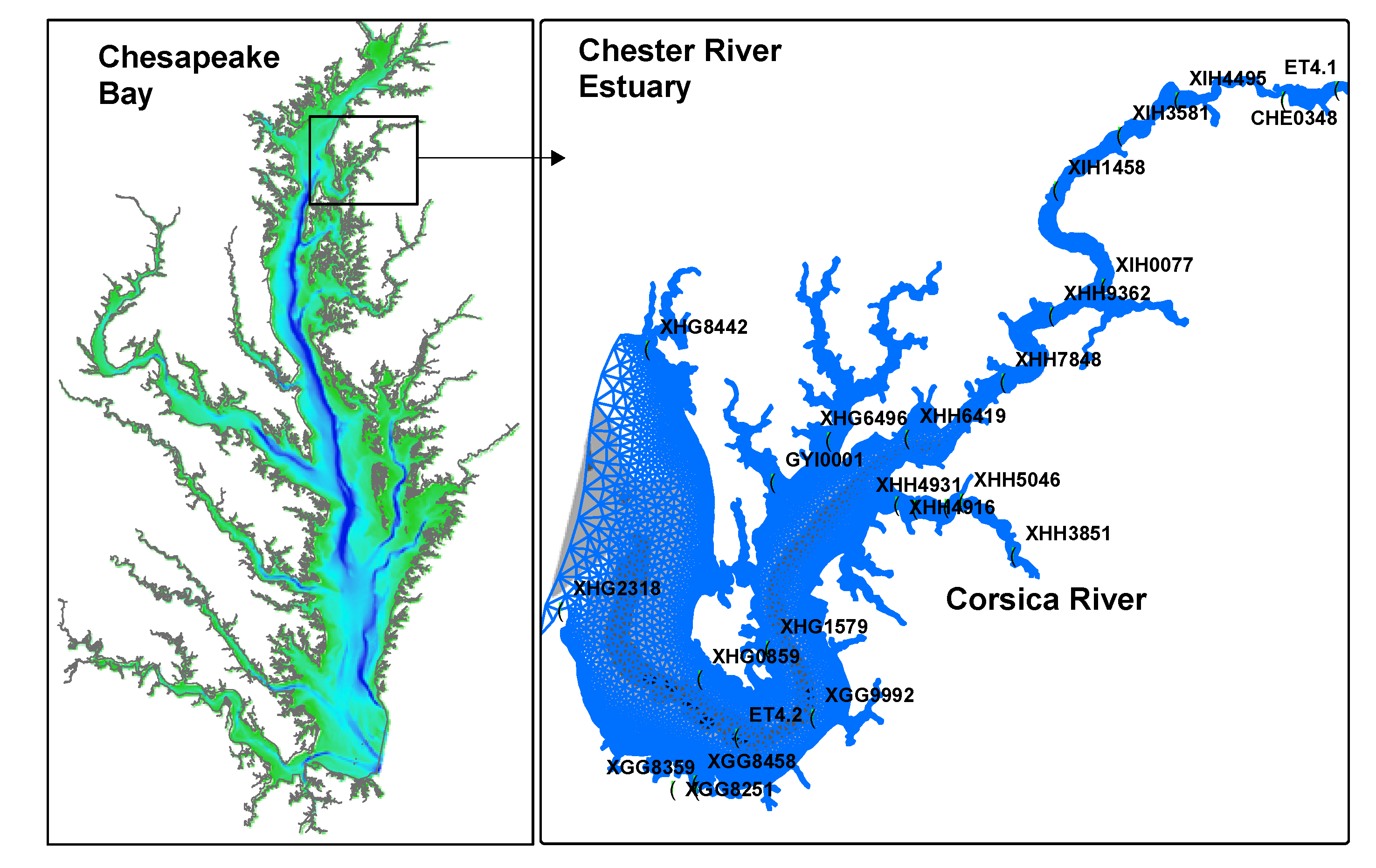
The simulation domain covers from the fall line to the Chester River mouth (Figure 1). Grid resolution varies from 1 km at the river mouth to 100 m near the coastline, with 13,824 cells in total, 8351 nodes, and 10 vertical sigma layers. The simulation time step was set at 5 s. The model was first spun up for 5 years using the forcing and currents of 2002. Initial condition was based on the EPA regulatory model CH3D-ICM simulation of the whole Chesapeake Bay (see the following section). Following the spinning up, the model was continuously run from 2002 to 2011.
2.2. Forcing Data
ICM uses the FVCOM computed currents and turbulence diffusivity fields to drive the water quality simulation [39]. In addition to the physical forcing, ICM needs shortwave radiation for photosynthesis and wind speed to determine the DO reaeration at the sea surface. Wind speed data were from the NOAA Thomas Point Buoy (38°53′56″ N 76°26′9″ W) located in the northern part of the Chesapeake Bay close to the Chester River estuary, and shortwave radiation data were downloaded from the North America Regional Reanalysis (NARR) ftp site (ftp://ftp.cdc.noaa.gov/Datasets/ NARR). A factor of 0.47 was applied to shortwave radiation to convert to Photosynthetically Active Radiation (PAR), including reflection at the sea surface [46]. NARR provided data with 3 h intervals and a linear interpolation was conducted during the simulation.
Fall line data of nutrient loading was generated using the regulatory watershed model HSPF calibrated with data collected at the USGS River Input Monitoring (RIM) stations on the Chesapeake Bay watershed. The annual total nitrogen loading to the Chester River domain ranged from 0.8 to 2.5 × 10⁶ kg with an average of 1.5 × 10⁶ kg, and that of phosphorus ranged from 30 to 178 × 103 kg with an average of 117 × 103 kg. Open boundary conditions at the river month were based on the CH3D-ICM simulation. The CH3D-ICM simulations were calibrated over the entire Chesapeake Bay from 2001 to 2011 with extensive monitoring data from the Chesapeake Bay Program. State variables at the Chester River open boundary nodes were recorded hourly. As CH3D-ICM and FVCOM-ICM shared the same nodes at the Chester River mouth, the CH3D-ICM outputs were directly used for the FVCOM-ICM simulation without horizontal interpolation. However, CH3D-ICM uses a z-coordinate in the vertical, and a linear interpolation was performed to bring the boundary data from the CH3D-ICM z-layers to the FVCOM-ICM sigma layers. As the FVCOM-ICM uses a smaller time step (5 s) as compared to the CH3D-ICM output (hourly), a linear interpolation in time was also performed during the simulation.
2.3. Observation Data and Statistical Analysis
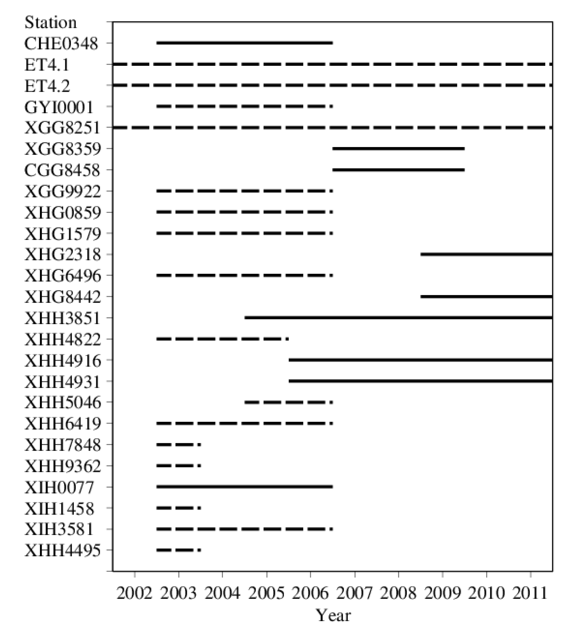
The Chesapeake Bay Program has maintained a monitoring program over the entire Bay since 1984. Two of the long-term monitoring stations are in the Chester River domain: ET4.2 in the mesohaline region (salinity 10–18 psu), and ET4.1 in the tidal fresh area (salinity <0.5 psu; Figure 1). Data of DO and chlorophyll from monthly (in winter) and biweekly (summer) cruises are available for the entire simulation period from 2002 to 2011 (Figure 2). The Department of Natural Resource (DNR) of Maryland also undertakes monitoring activities in the Maryland portion of the Bay, including the Chester River and the Corsica River in the simulation domain. Some of the stations are occupied in long terms, such as XGG8251 located on the southern bank of the Chester River estuary (Figure 1), but most of the DNR monitoring stations are rotational, occupied during certain years. There were 23 stations sampled during the simulation period in the DNR monitoring programs and data availability and duration are depicted in Figure 2.
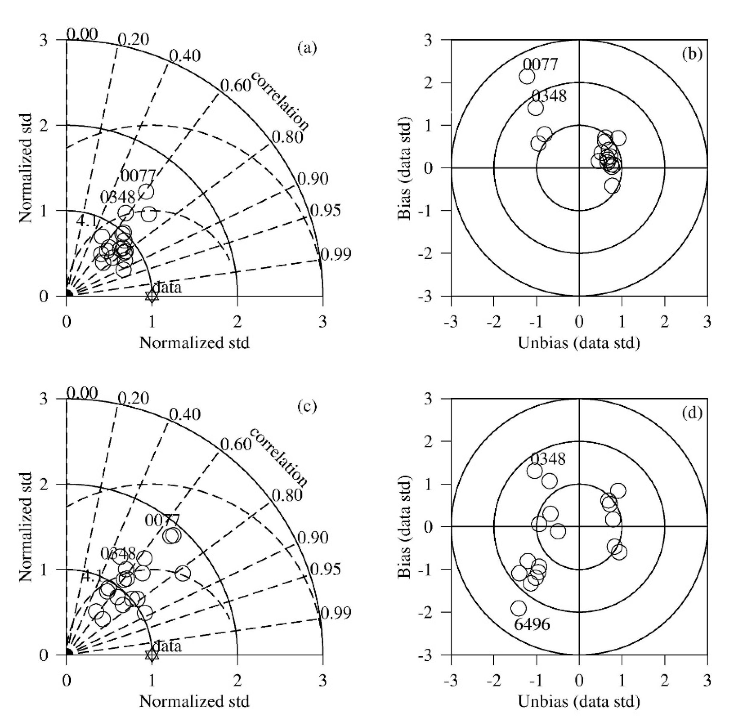
In addition to cruise-based monitoring programs, DNR conducted Continuous Monitoring programs (CMON) at nine of the monitoring stations (solid line in Figure 2). These are high-frequency (every 15 min) data based on electronic sensor measurements, and tele-communicated to land-based laboratories. The sensors were carefully calibrated on a monthly basis with bottle sample analysis. All these data were used for model calibration and validation. Time-series plots, Taylor Diagrams, and Target Diagrams were employed for simulation-observation comparison, and Principal Component Analysis (PCA) and Generalized Additive Model (GAM) were used for model results analysis. These methods were described in [39], where readers are referred to for more information. Briefly, Taylor diagrams depict the comparison between simulations and observations in terms of the correlation coefficient, the standard deviation of both the simulation and the observation, and the centered root mean squared error (CRMSE) on the same diagram [47,48]. The angle from zero indicates the correlation between simulation and observation, and the distance from the origin is the normalized standard deviation (std) of the simulated values (simulation std divided by observation std), with the result that the overall distance between the observation and the simulation on the Taylor diagram is the CRMSE. Note that the correlation coefficient (R) is used in the Taylor diagram whereas the coefficient of determination (R2) is often referred to in statistical analyses. In the Target diagram, the bias (the difference between the simulation mean and the observation mean) is scaled on the y axis and the centered mean squared error (unbias) on the x axis, and as a result the total bias (the root mean squared error, RMSE) is the radial distance from the origin to the data point [48,49]. As in the Taylor diagram, the bias and the CRMSE are normalized to the data standard deviation. The combined Taylor and Target diagram can thus give a comprehensive assessment of the simulation by providing the correlation coefficient, standard deviation, the centered mean squared error, the bias, and the total RMSE (see “Results” section for graphic examples). The correlation coefficient essentially compares the timing of phytoplankton blooms and the seasonality of biogeochemical events, the bias compares the magnitudes and CRMSE compares the variability between simulation and observation. Harding et al. [50] found that GAM is suitable to extract long-term trend, interannual and seasonal variations from time series data, which was adopted in this paper. Principal component analysis (PCA) is a type of linear transformation through which principal dimensions are found in the variable space that explain the covariance among the variables [51].
3. Results
3.1. Comparison between Simulation and Observation
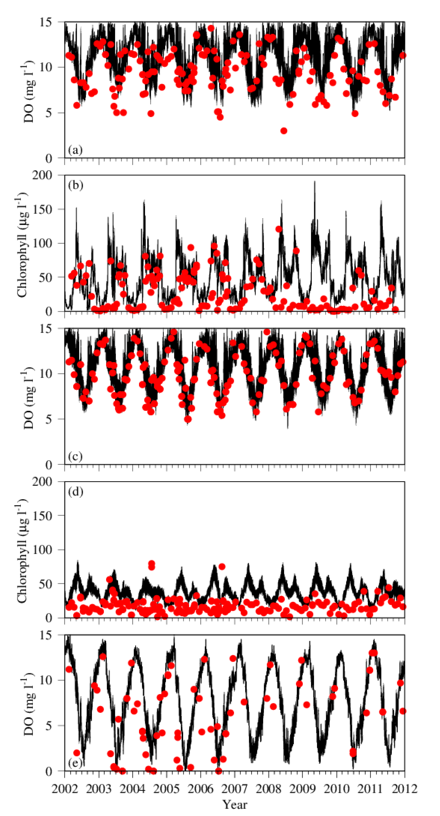
Data of dissolved oxygen and chlorophyll collected at 24 stations were used to assess the robustness of the simulation. Given the large quantity of data, only the most representative stations are plotted in time-series (Figure 3): ET4.1 in the tidal fresh zone with shallow water depth (3 m), and ET4.2 in the central part of the mesohaline region in the deep channel of the lower estuary (Figure 1). These two stations are part of the long-term monitoring network of the Chesapeake Bay Program and thus have the most complete data set over the simulation period. Data from other stations occupied during the Maryland state monitoring programs were included in the statistical analysis of the Taylor and Target diagrams.
Given the shallow depth at Station ET4.1, only the surface layer is presented (Figure 3a,b). The time series of DO was dominated by seasonal cycle both in the observation and simulation, with high values in winter and low values in summer and transitional in spring and fall (Figure 3a). In addition to the seasonal cycles, the model revealed significant high-frequency variations in DO at a diurnal scale. In some years, the model tended to overestimate DO concentration at both the high and low ends. A particularly low value of DO (ca. 3 mg L−1) was observed in May 2008, which was not produced in the model simulation. The minimum values of DO in 2003 and 2004 were also lower in the observation than in the simulation.
In the chlorophyll time series data at Station ET4.1, (Figure 3b), two peaks of concentration were observed and simulated in most of the years: one in April and another in October. This indicates two phytoplankton blooms in the region: spring bloom in April and fall bloom in October. The spring phytoplankton bloom had a higher amplitude with chlorophyll concentration up to 150 to 200 µg L−1, whereas the fall bloom had a relatively lower amplitude with chlorophyll concentration close to 100 µg L−1. The lowest values were reached during the winter season between two successive years. High-frequency variations superposed on the seasonal cycle were also reproduced in the chlorophyll concentration as well as in the DO concentration. In most of the cases, the model simulation compared reasonably well with the observation. In 2009, however, the observation did not show pronounced blooms, whereas the model predicted two blooms as in other years. Additionally, the spring phytoplankton bloom was missing in the observation in 2010 and 2011 but was generated in the simulation.
DO at Station ET4.2 was also dominated by large seasonal variations, with high values in winter and spring, and low values in summer and fall (Figure 3c). The highest values were mostly found in spring during the phytoplankton bloom. At this station, the model simulation of DO compared well with the observation in both the timing and amplitude of the seasonal cycles. The model predicted two phytoplankton blooms at this station as well (Figure 3d), but with an amplitude much smaller than that at Station ET4.1. The spring bloom reached about 70 µg L−1 in chlorophyll concentration and about 50 µg L−1 for the fall bloom, which were less than half of the amplitudes at Station ET4.1. DO simulation in the bottom layer also compared well with the observation (Figure 3e). The amplitude of seasonal variation in the bottom DO was even higher than that in the surface layer, ranging from 0 to 15 mg L−1.
Taylor Diagrams and Target Diagrams were constructed on DO simulation at all the observation stations (Figure 4). For surface DO, most of the stations had a correlation coefficient between simulation and observation >0.6 and the centered mean squared error <1 standard deviation of the observation (Figure 4a). Stations 0348 and ET4.1 had a correlation coefficient lower than 0.6 and Station 0077 had a centered root mean squared error higher than 1. These stations are all located in the tidal fresh zone where DO concentration is relatively high (>2 mg L−1, the critical value for hypoxia). As show in Figure 3a, the model tended to overestimate DO concentration at both the high and low ends in the DO concentration range, which may explain the lower statistical numbers. On the Target diagram (Figure 4b), most of the stations had a total root mean squared error (RMSE) lower than or close to 1 standard deviation of the observation. Again, Stations 0077 and 0348 were outliers with a total RMSE higher or close to 2. At these two stations, the model tended to overestimate the mean of DO concentration. Similar results were obtained for the bottom layer (Figure 4c,d). Most of the stations had a correlation coefficient >0.6 and a centered RMSE less than 1. Stations 0348 and ET4.1 were among the stations with a lower correlation coefficient (<0.6) and Station 0077 had a relatively larger centered RMSE. On the Target Diagram, most of the stations had a total RMSE <1, with some other stations being between 1 and 2. Station 6496 was an outlier with a total RMSE higher than 2. Both the mean and the variability were underestimated by the model at this station. This station is in a secondary tributary on the northern bank of the Chester River and it is unlikely that it can significantly contribute to the total hypoxia volume in the entire Chester River estuary.
3.2. Seasonality and Interannual Variations in Hypoxia Volume
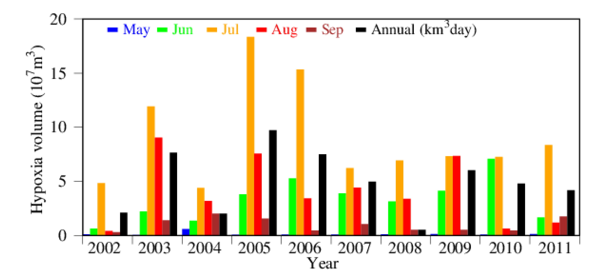
Hypoxia is defined as a condition of low dissolved oxygen (<2 mg L−1) in a marine environment [1,2,9,52]. Instantaneous and monthly average of hypoxia was given in total volume in the Chester River estuary, while interannual variations were expressed as hypoxia volume-days, i.e., the sum of daily hypoxia volume over the entire year. The timing of hypoxia occurrence can differ from year to year so that changes in daily and monthly hypoxia volume can be caused by shifting in time of the hypoxia occurrence. Hypoxia volume-days integrate all the hypoxia occurrences during the entire year so that it is less subject to changes in the seasonality of hypoxia events. The year 2005 had the highest hypoxia volume-days (black bar in Figure 5), followed by 2003 and 2006, whereas 2008 had the lowest hypoxia volume-days among the 10 simulated years. Additionally, 2002 and 2004 had relatively low hypoxia volume-days compared to the average of the 10 simulated years. On a monthly basis, July had the highest hypoxia volume in most of the simulated years, except in 2009 when August’s hypoxia volume was slightly higher than that of July. In 2010, the hypoxia volume was almost identical in June and July. Hypoxia started in June and lasted till September in 2009, whereas in 2002, only July had a significant amount of hypoxia. Hypoxia volume in July 2005 was the highest among all the simulated years and months.
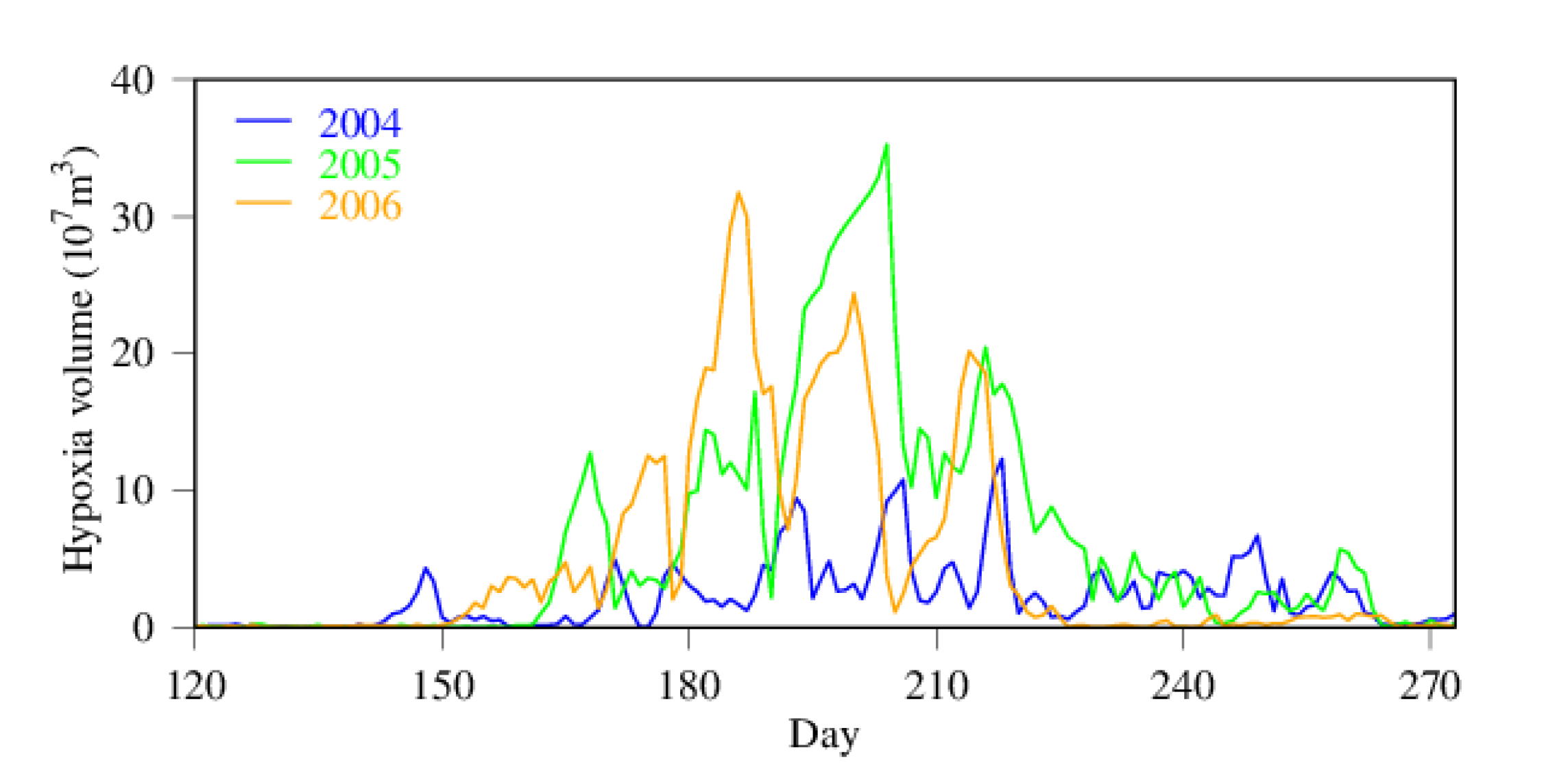
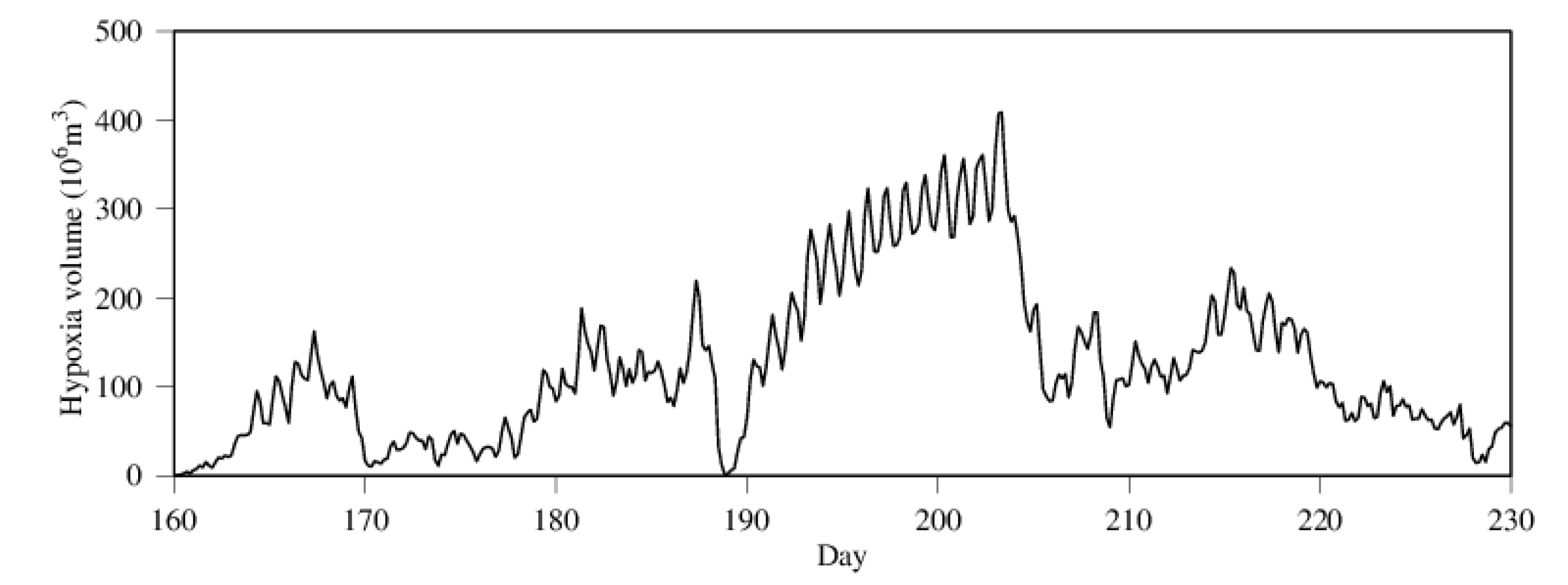
Daily hypoxia volume is depicted in Figure 6 for 2004 through 2006, with 2004 as an example of low hypoxia years and the other two years as examples of high hypoxia years. Hypoxia did not widely spread in 2004, with only sporadic hypoxic events with limited amplitude. There was a huge hypoxic event during the entire month of July in 2005, leading to a year of high hypoxia volume-days, while moderate hypoxic events occurred from June through August in 2006. Hypoxia occurrence differs from year to year with interruptions between hypoxic events. Hypoxia volume has diurnal variability as well (Figure 7). Diurnal changes in hypoxia volume can reach the order of 1.0 × 10⁸ m3 in the Chester River estuary, amounting to about one quart to one third of the total hypoxia volume. Note that there was an abrupt decrease in hypoxia volume near the end of July 2005 (day 202–206).
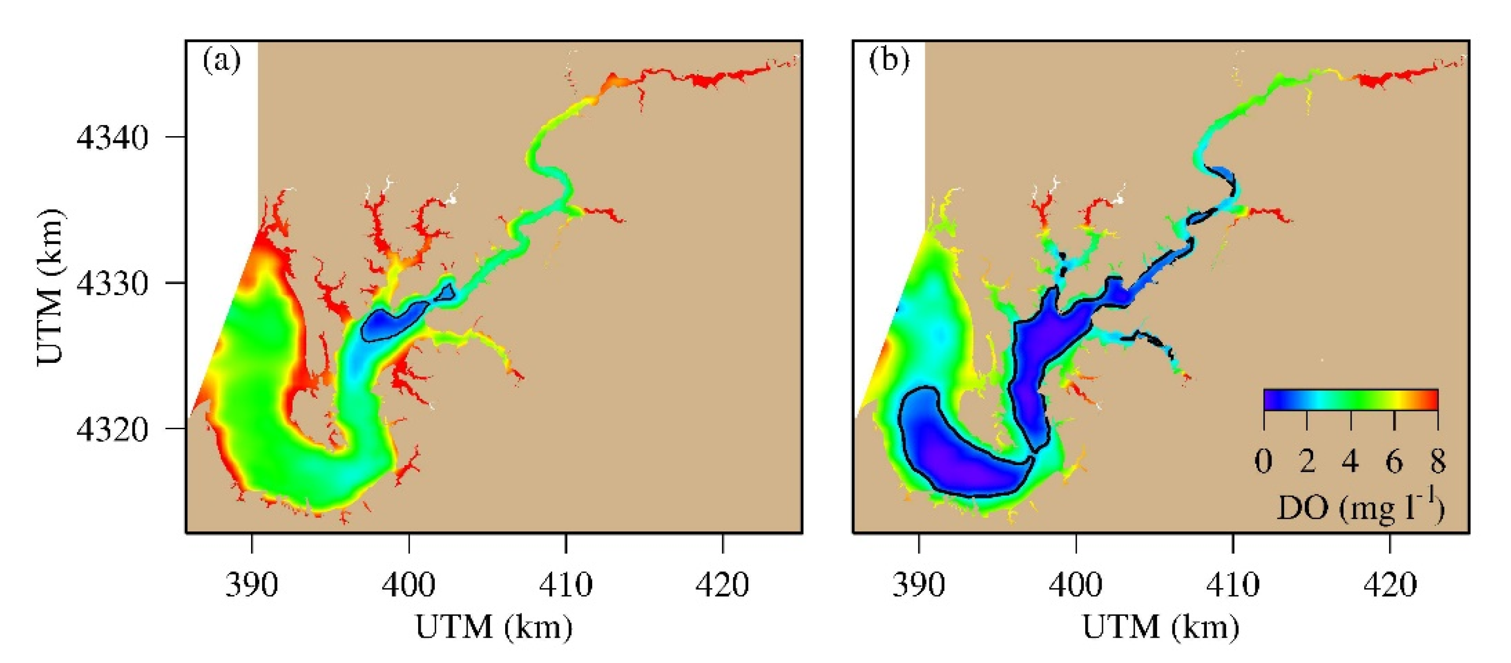
The spatial distribution of bottom DO in June 21 is depicted as an example of low hypoxia day and in July 21 as an example of high hypoxia day in 2005 (Figure 8). In June 21, only a small area in the deep channel adjacent to the Corsica River had bottom DO <2 mg L−1. In July 21, low DO <2 mg L−1 became widespread, from the lower estuary to the upper reach of the estuary. The core of hypoxia distribution is along the main deep channel. What is interesting is that hypoxia distribution is discontinued at several curvatures of the main channel. The bathymetry did not show similar discontinuity in a similar manner at the same location. It is most likely linked to other mechanisms that have the potential to alter DO concentration in the bottom layer.
3.3. GAM Decomposition of Time-Series Hypoxia Volume and PCA Causality Analysis
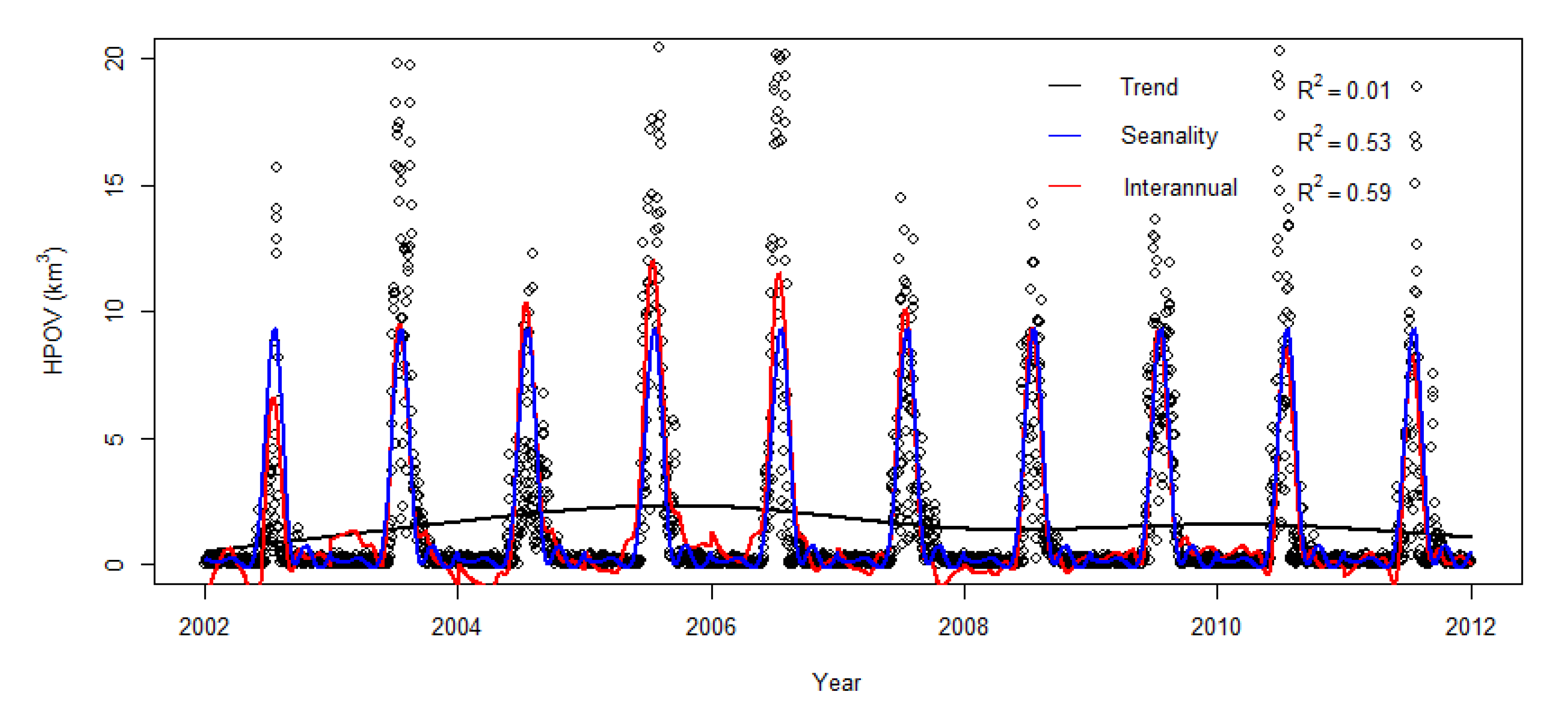
General additive models were fitted to the daily hypoxia volume time series (Figure 9). No general trend was found. The hypoxia time series is dominated by seasonal variations, with seasonal model accounting for 53% of the total variance. Most of the hypoxia occurred within a relatively short period of time in June and July. Adding interannual variations resulted in a fitted function that explains 59% of the total variance. The prediction of the interannual function (red curve, Figure 9) was higher than the seasonal curve from 2004 to 2006 by about 4 km3, indicating that hypoxia was significantly higher in these three successive years than in other years. On the other hand, the interannual variation line is below the seasonal prediction (blue line) in 2002 by about 4 km3, indicating that hypoxia was particularly low in 2002. These differences are based on the prediction of the fitted interannual GAM function. The maximum hypoxia volume reached 20 km3 in 2005, but only about 12 km3 in 2004.
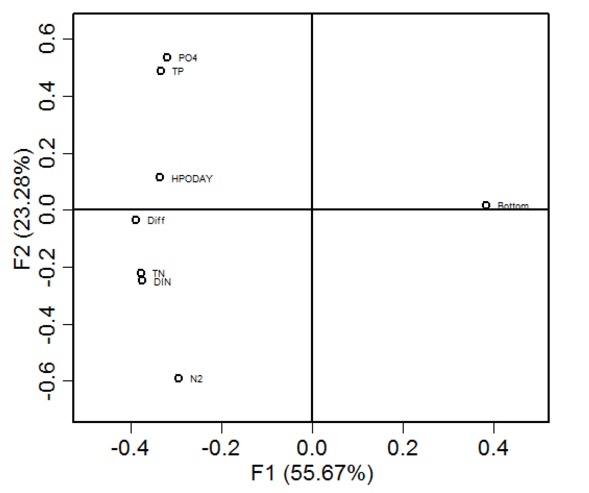
Principal component analysis (PCA) was conducted on the daily data of total hypoxia volume (HPOV), nutrient loads including dissolved inorganic nitrogen (DIN), total nitrogen (TN), phosphate (PO4) and total phosphorus (TP), bottom saltwater intrusion distance (Bottom), difference between bottom and surface saltwater intrusion (Diff), and stratification using the Brunt–Väisälä frequency (N2). The N2 was the daily average on the along-channel transect. The first principal component explained 56% of the total variance (x axis in Figure 10) and the second accounted for another 23% of the total variance (y axis in Figure 10). As such, the first two principal components explained 79% of the total variance. All the variables had high loadings on the first principal component and were thus relevant to the hypoxia development. Except the bottom saltwater intrusion distance, all other variables were located on the same side as HPOV on the first principal component, indicating their positive relationships with hypoxia occurrence. On the second principal component, PO4 and TP were located on the same side as HPOV whereas DIN and TN were on the opposite side, indicating that phosphorus loads have more impact on the hypoxia development than nitrogen loads in the Chester River estuary. Both the stratification N2 and Diff were loaded on the same side as the HPOV on the first principal component, indicating their positive impact on hypoxia development. However, saltwater intrusion had a negative relationship with HPOV.
4. Discussion
4.1. Time-Series Pattern
The seasonal cycle of DO is due to changes in the solubility of DO in response to changes in water temperature and changes in biological and biogeochemical processes. Water temperature ranges from 1 °C in winter to about 30 °C in summer [38]. Based on the DO saturation formulation of Garcia and Gordon, [42] used in the model and assuming a salinity value of 2 psu at Station ET4.1, the DO saturation concentration varies from 14.0 mg L−1 at 1 °C to 7.5 mg L−1 at 30 °C., i.e., the saturation concentration at 1 °C is almost double that at 30 °C. The simulated variation in DO concentration ranges from 5 to 15 mg L−1, which is larger than the changes in solubility. This extra seasonal variation in DO concentration is linked to seasonal shifts in biological and biogeochemical dynamics. Spring is dominated by phytoplankton blooms, which produce oxygen and lead to supersaturation in DO concentration. Summer and early fall are dominated by remineralization of organic substances, which consume DO and lead to under-saturation in DO concentration. The diurnal variations on top of the seasonal cycles are due to the diurnal cycle between phytoplankton photosynthesis during the daytime and respiration and remineralization during the night. Other mechanisms that can lead to high-frequency variations are heterogeneity in the water property, such as DO concentration and phytoplankton abundance, and horizontal advection. Tide and river flow continuously move water mass through a fixed station such as ET4.1, and differences in water property will lead to variations in observation and simulation at a fixed station.
The amplitude of seasonal variability in bottom DO at ET4.2 is even higher than that in the surface layer, ranging from 0 to 15 mg L−1. In addition to changes in solubility, stratification is another factor affecting DO concentration in the bottom layer. During the winter season when the water column is quasi-homogeneous, bottom water is mostly mixed with surface water with a high DO concentration. During the summer season when the water column is stratified, bottom water is stagnated with little convection or mixing with the surface layers. Moreover, high temperature and abundant organic substances produced by the spring phytoplankton bloom contribute to the increased remineralization and thus DO depletion in summer, amplifying the seasonal variations in bottom DO. The high similarity between bottom DO observation and simulation provides sound basis for robust model prediction of hypoxia volume.
4.2. Major Drivers of Hypoxia Occurrence
PCA causality analysis revealed that nutrient loads are the major driver of hypoxia development in the Chester River estuary. This agrees with previous studies conducted in the entire Chesapeake Bay where nutrient loading is found to be the dominating factor in determining interannual variability in hypoxia occurrence [16,22]. However, phosphorus and nitrogen loads do not have equal impact. Phosphorus loads have a higher effect than nitrogen loads on hypoxia development in the Chester River estuary. This is due to the difference in limitation between the two types of nutrient elements. Usually phosphorus is more limiting in terrestrial environments, whereas nitrogen is the essential limiting factor in the ocean [20]. Estuaries are transitional zones where the relative limiting effect can vary in space and time [53,54]. In the Chester River estuary, phosphorus is more of a limiting factor than nitrogen. Consequently, phosphorus loads have more impact on hypoxia development than nitrogen. This has an important implication in nutrient management and related decision making. Phosphorus load reduction will be more efficient than nitrogen in water quality restoration in the Chester River estuary. On top of nutrient loads, stratification and saltwater intrusion turned out to be significant factors in determining hypoxia occurrence in the Chester River estuary. Both the Brunt–Väisälä frequency (N2) and the difference between bottom and surface saltwater intrusion distances reflect stratification of the water column. The negative relationship between stratification and bottom water saltwater intrusion means that stronger saltwater intrusion leads to less stratification and less hypoxia. When saltwater intrusion extended to the oligohaline zone (salinity 0.5–10 psu) in the middle portion of the Chester River estuary where water depth is relative shallow, bottom friction can cause strong vertical mixing and reduce the overall average of stratification along the main stem and less hypoxia development.
4.3. Spatial Distribution of Hypoxic Water
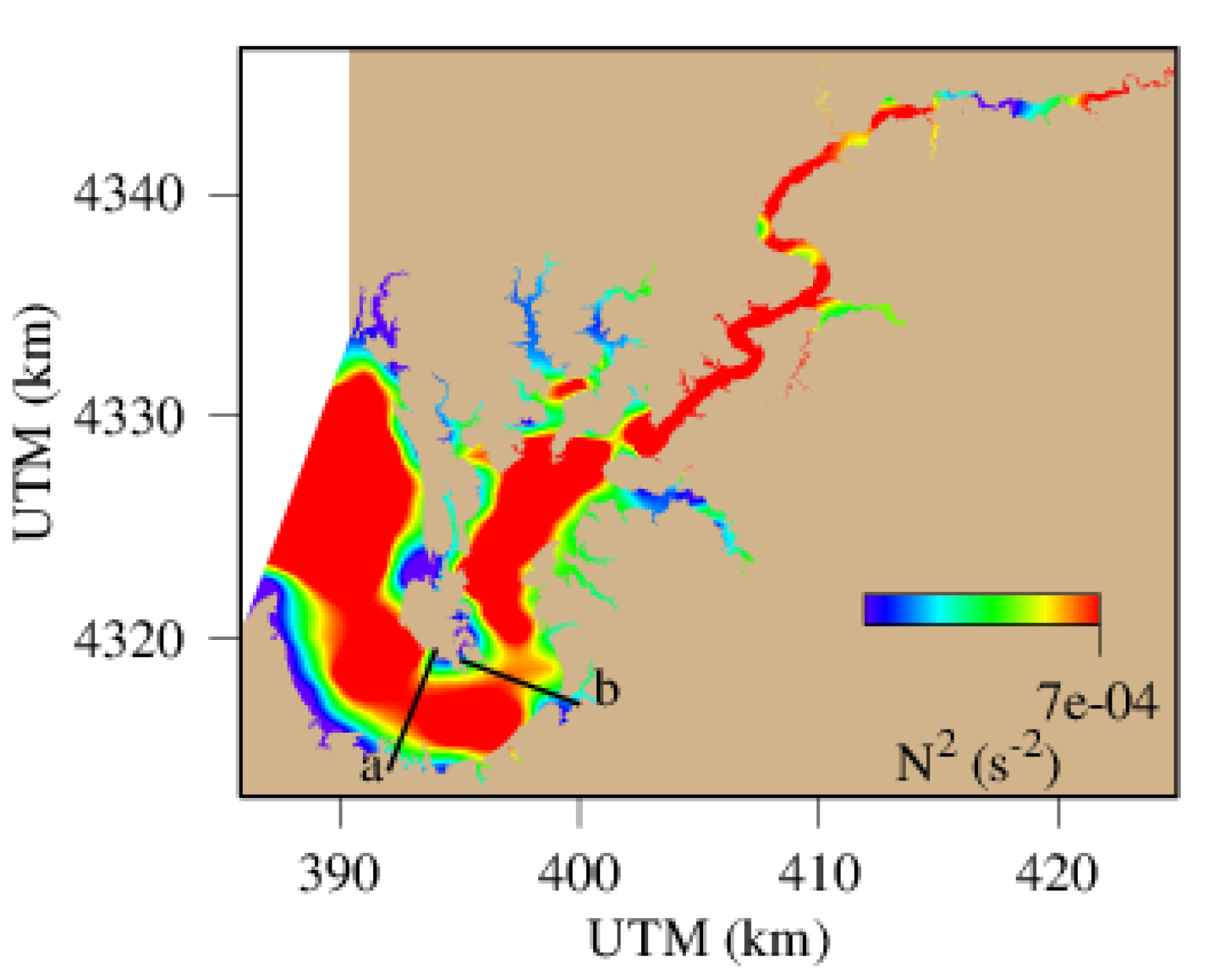
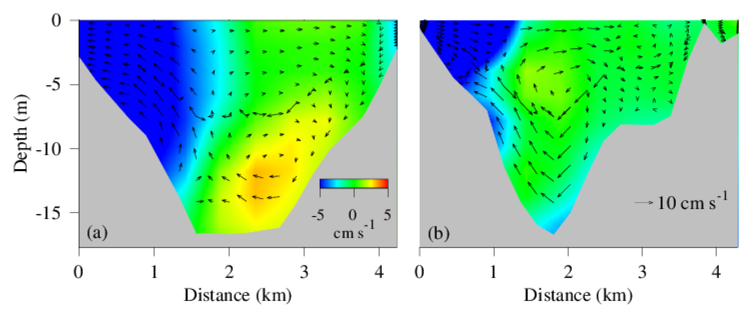
Figure 8b shows the spatial distribution of hypoxic water with DO < 2 mg L−1, and there is a major discontinuity at the curvature of the main stem. Similarly, the stratification metric N2 is also relatively low at the same location and time (Figure 11). At meandering points, the water momentum and centrifugal force lead to the formation of helical circulation that can strengthen lateral circulation and vertical convection [38,55,56,57,58]. Indeed, there is stronger lateral circulation on the transect at the curvature where hypoxia distribution is interrupted (Figure 12b). In the surface layer, water moves toward the right-hand shore (the outside bank of the meandering), which is in the opposite direction of the Coriolis force, but in the direction of the centrifugal force. Consequently, the outside bank of the curvature becomes a convergent zone whereas the inside bank a divergent zone, which subsequently generate cross channel circulation with elevated vertical vectors in the circulation field. On the other transect downstream of the meandering where the main channel is relatively straight, water mass mostly moves to the left side (looking up stream), in agreement with the Coriolis force. The major meandering of the main channel at the lower Chester River estuary causes helical circulation, enhances vertical convection and mixing, weakens stratification, and improves DO concentration and hypoxia occurrence.
5. Conclusions
The model simulation shows that hypoxia is the most severe in July in the Chester River, followed by August and June, whereas there is limited extension in hypoxia occurrence in May and September. The timing of the hypoxia occurrence changes from year to year, but mostly within the three-month window from June to August. In 2010, the total hypoxia volume in June was as high as in July and in 2009, the total hypoxia volume was even slightly higher in August than in July. Most of the hypoxia occurred in the main stem along the deep channels, with limited occurrence in the Corsica River and other sub-tributaries. The Chester River estuary is characterized by several meanders and it has been found that helical circulation is formed at certain curvatures due to the centrifugal force exerted on running water. The helical lateral circulation creates vertical convective vectors, reduces stratification, enhances exchange between the surface and bottom layers, and as such reduces the occurrence of hypoxia at certain locations. Hypoxia was the most severe in 2005 and the lowest in 2004. Statistical analysis shows that nutrient loading is the dominating factor in determining the extension and severity of hypoxia in the Chester River estuary, followed by stratification and saltwater intrusion. It has been found that phosphorus loads have more impact on hypoxia occurrence than nitrogen in the Chester River estuary due to its higher limiting effect on phytoplankton development. Consequently, phosphorus load reduction will be more efficient than nitrogen load reduction in restoration efforts.
Funding
This research was funded by the US Environmental Protection Agency (grant number CB-75230480) and the APC was funded by the Integration and Application Network, University of Maryland Center for Environmental Science.
Acknowledgments
The author thanks the Chesapeake Bay Program and the Maryland Department of Natural Resource for providing the observation data and Florence R. Tian for English edits. Special thanks go to the Chesapeake Bay Program Modeling Team for their enthusiastic helps, particularly Lewis Linker, Gary Shenk, Ping Wang, Gopal Bhatt, Bill Dennison, and Dave Nemazie. Comments from the editor and two reviewers were appreciated.
Conflicts of Interest
The authors declare no conflict of interest.
References
- Renaud, M.L. Hypoxia in Louisiana coastal waters during 1983: Implications for fisheries. Fish. Bull. 1986, 84, 19–26. [Google Scholar]
- Diaz, R.J. Overview of hypoxia around the world. J. Environ. Qual. 2001, 30, 275–281. [Google Scholar] [CrossRef] [PubMed]
- Rabalais, N.N.; Turne, R.E.; Wiseman, W.J. Gulf of Mexico hypoxia, aka “The dead zone”. Ann. Rev. Ecol. Syst. 2002, 33, 235–263. [Google Scholar] [CrossRef]
- Diaz, R.J.; Rosenberg, R. Spreading dead zones and consequences for marine ecosystems. Science 2008, 321, 926–929. [Google Scholar] [CrossRef]
- Howarth, R.F.; Chan, D.J.; Conley, J.; Garnier, S.C.; Doney, R.M.; Billen, G. Coupled biogeochemical cycles: Eutrophication and hypoxia in temperate estuaries and coastal marine ecosystems. Front. Ecol. Environ. 2011, 9, 18–26. [Google Scholar] [CrossRef] [Green Version]
- Rabalais, N.N.; Cai, W.J.; Carstensen, J.; Conley, D.J.; Fry, B.; Hu, X.; Quiñones-Rivera, Z.; Rosenberg, R.; Slomp, C.P.; Turner, R.E.; et al. Eutrophication-driven deoxygenation in the coastal ocean. Oceanography 2014, 27, 172–183. [Google Scholar] [CrossRef] [Green Version]
- Hale, S.S.; Cicchetti, G.; Deacutis, C.F. Eutrophication and hypoxia diminish ecosystem functions of benthic communities in a New England estuary. Front. Mar. Sci. 2016, 3. [Google Scholar] [CrossRef] [Green Version]
- Raballais, N.N.; Turner, R.E.; Wiseman, W.J., Jr. Hypoxia in the Gulf of Mexico. J. Environ. Qual. 2001, 30, 320–329. [Google Scholar] [CrossRef]
- Zhang, J.; Gilbert, D.; Gooday, A.J.; Levin, L.; Naqvi, S.W.A. Natural and human-induced hypoxia and consequences for coastal areas: Synthesis and future development. Biogeosciences 2010, 7, 1443–1467. [Google Scholar] [CrossRef] [Green Version]
- Manuel, J. Nutrient pollution: A persistent threat to waterways. Environ. Health Perspect. 2014, 122, 304–309. [Google Scholar] [CrossRef] [Green Version]
- Larsen, C.E. The Chesapeake Bay: Geologic product of rising sea level. USGS Fact Sheet 1998, 1–12, 102–198. [Google Scholar]
- Boynton, W.R. Chesapeake Bay eutrophication Current status, historical trends, nutrient limitation and management actions. In Proceedings of the Coastal Nutrients Workshop, Australian Water & Wastewater Association Incorporated, Artamon, Australia, 30–31 October 1997; pp. 6–13. [Google Scholar]
- Murphy, R.R.; Kemp, W.M.; Ball, W.P. Long-term trends in Chesapeake Bay seasonal hypoxia, stratification, and nutrient loading. Estuar. Coasts 2011, 34, 1293–1309. [Google Scholar] [CrossRef]
- Sale, J.W.; Skinner, W.W. The vertical distribution of dissolved oxygen and the precipitation by saltwater in certain tidal areas. J. Franklin I. 1917, 184, 837–848. [Google Scholar] [CrossRef]
- Newcombe, C.L.; Horne, W.A. Oxygen-poor waters of the Chesapeake Bay. Science 1938, 88, 80–81. [Google Scholar] [CrossRef] [PubMed]
- Hagy, J.D.; Boynton, W.R.; Keefe, C.W.; Wood, K.V. Hypoxia in Chesapeake Bay, 1950-2001: Long-term change in relation to nutrient loading and river flow. Estuaries 2004, 27, 634–658. [Google Scholar] [CrossRef]
- Rothschild, B.J.; Ault, J.S.; Goulletquer, P.; Heral, M. Decline of the Chesapeake Bay oyster population: A century of habitat destruction and overfishing. Mar. Ecol. Prog. Ser. 1994, 111, 29–39. [Google Scholar] [CrossRef]
- Breitburg, D.L.; Hondorp, D.W.; Davias, L.A.; Diaz, R.J. Hypoxia, nitrogen, and fisheries: Integrating effects across local and global landscapes. Annu. Rev. Mar. Sci. 2009, 1, 329–349. [Google Scholar] [CrossRef] [Green Version]
- Schubel, J.R.; Pritchard, D.W. Responses of upper Chesapeake Bay to variations in discharge of the Susquehanna River. Estuaries 1986, 9, 236–249. [Google Scholar] [CrossRef]
- Kemp, W.M.; Boyton, W.R.; Adolf, J.E.; Boesch, D.F.; Boicourt, W.C.; Brush, G.; Cornwell, J.C.; Fisher, T.R.; Gilbert, P.M.; Hagy, J.D.; et al. Eutrophication of Chesapeake Bay: Historical trends and ecological interactions. Mar. Ecol. Prog. Ser. 2005, 303, 1–29. [Google Scholar] [CrossRef]
- Kemp, W.M.; Testa, J.M.; Conley, D.J.; Gilbert, D.; Hagy, J.D. Temporal responses of coastal hypoxia to nutrient loading and physical controls. Biogeosciences 2009, 6, 2985–3008. [Google Scholar] [CrossRef] [Green Version]
- Li, M.; Lee, Y.J.; Testa, J.M.; Li, Y.; Ni, W.; Kemp, W.M.; Di Toro, D.M. What drives interannual variability of hypoxia in Chesapeake Bay: Climate forcing versus nutrient loading? Geophys. Res. Lett. 2016, 43, 2127–2134. [Google Scholar] [CrossRef] [Green Version]
- Scully, M.E. Wind modulation of dissolved oxygen in Chesapeake Bay. Estuar. Coasts 2010, 33, 1164–1175. [Google Scholar] [CrossRef]
- Testa, J.M.; Li, Y.; Lee, Y.J.; Li, M.; Brady, D.C.; Di Toro, D.M.; Kemp, W.M.; Fitzpatrick, J.J. Quantifying the effects of nutrient loading on dissolved O2 cycling and hypoxia in Chesapeake Bay using a coupled hydrodynamic–biogeochemical model. J. Mar. Syst. 2014, 139, 139–158. [Google Scholar] [CrossRef]
- Irby, I.D.; Friedrichs, M.A.M.; Friedrichs, C.T.; Bever, A.J.; Hood, R.; Lanerolle, L.W.J.; Li, M.; Linker, L.; Scully, S.E.; Sellner, K.; et al. Challenges associate with modeling low-oxygen waters in Chesapeake Bay: A multiple model comparison. Biogeosciences 2016, 13, 2011–2028. [Google Scholar] [CrossRef] [Green Version]
- Xia, N.; Jiang, L. Application of an unstructured grid-based water quality model to Chesapeake Bay and its adjacent coastal ocean. J. Mar. Sci. Eng. 2016, 4, 52. [Google Scholar] [CrossRef] [Green Version]
- Jiang, L.; Xia, M. Wind effects on the spring phytoplankton dynamics in the middle reach of the Chesapeake Bay. Ecol. Model. 2017, 363, 68–80. [Google Scholar] [CrossRef]
- Kuo, A.Y.; Moustafa, M. Hypoxia in the Lower Rappahannock Estuary. In Special Report in Applied Marine Science and Ocean Engineering No. 302; W&M Publish, William and Mary College: Williamsburg, WV, USA, 1989; pp. 1–133. [Google Scholar]
- Sturdivant, S.K.; Brush, M.J.; Diaz, R.J. Modeling the effect of hypoxia on macrobenthos production in the Lower Rappahannock River, Chesapeake Bay, USA. PLoS ONE 2013, 8, e84140. [Google Scholar] [CrossRef]
- Breitburg, D.L.; Admack, A.; Rose, K.A.; Kolesar, S.E.; Decker, M.B.; Purcell, J.E.; Keister, J.E.; Cowan, J.H., Jr. The pattern and influence of low dissolved oxygen in the Patuxent River, a seasonally hypoxic estuary. Estuaries 2003, 26, 280–297. [Google Scholar] [CrossRef]
- Testa, J.M.; Kemp, W.M.; Boynton, W.R.; Hagy, J.D., III. Long-term changes in water quality and productivity in the Patuxent River estuary: 1985 to 2003. Estuar. Coasts 2008, 31, 1021–1037. [Google Scholar] [CrossRef] [Green Version]
- Kuo, A.Y.; Neilson, B.J. Hypoxia and salinity in Virginia estuaries. Estuaries 1987, 10, 277–283. [Google Scholar] [CrossRef]
- MDE. Watershed Report for Biological Impairment of Middle Chester River Watershed in Kent and Queen Anne’s Counties, Maryland; EPA Report, BSID Analysis; Middle Chester River: Annapolis, MD, USA, 2013; 33p. [Google Scholar]
- DNR. Maryland Chesapeake Bay Oyster Management Plan; DNR 17-012319-117; Maryland Department of Natural Resource: Annapolis, MD, USA, 2019.
- Cooney, J.J.; Martin, F.D.; Roosenberg, W.H.; Freeman, D.H.; Bostater, C.R. An Evaluation of Chester River Oyster Mortality; MDDNR: Annapolis, MD, USA, 1990; 129p. [Google Scholar]
- Boynton, W.R.; Testa, J.M.; Kemp, W.M. An Ecological Assessment of the Corsica River Estuary and Watershed: Scientific Advice for Future Water Quality Management; CBL 09-117; UMCES: Cambridge, MD, USA, 2009. [Google Scholar]
- Leight, A.; Jacobs, J.; Gonsalves, L.; Messick, G.; McLaughpin, S.; Lewis, J.; Brush, J.; Daniels, E.; Rhodes, M.; Collier, L.; et al. Coastal Ecosystem Assessment of Chesapeake Bay Watershed: A Story of Three Rivers–The Corsica, Magothy and Rhode; NOAA Technical Memorandum NOS NCCOS 189; NOAA: Silver Spring, MD, USA, 2014; 93p. [Google Scholar]
- Tian, R.C. Factors controlling saltwater intrusion across multi-time scales in estuaries, Chester River, Chesapeake Bay. Estuar. Coast. Shelf Sci. 2019, 223, 61–73. [Google Scholar] [CrossRef]
- Cerco, C.F.; Noel, M.R. The 2002 Chesapeake Bay Eutrophication Model; US EPA report 903-R-04-004; US Army Corps of Engineers, Waterways Experiment Station: Washington, DC, USA, 2004. [Google Scholar]
- Sanderson, B.G.; Redden, A.M.; Evens, K. Grazing constants are not constant: Microzooplankton grazing is a function of phytoplankton production in an Australian lagoon. Estuar. Coasts 2012, 35, 1270–1284. [Google Scholar] [CrossRef]
- Jassby, A.; Platt, T. Mathematical formulation of the relationship between photosynthesis and light for phytoplankton. Limnol. Oceanogr. 1976, 21, 540–547. [Google Scholar] [CrossRef] [Green Version]
- Garcia, H.W.; Gordon, L.I. Oxygen solubility in seawater: Better fitting equations. Limnol. Oceanogr. 1992, 37, 1307–1312. [Google Scholar] [CrossRef]
- Morel, F. Principles of Aquatic Chemistry; John Wiley and Sons: New York, NY, USA, 1983; 150p. [Google Scholar]
- DiToro, D.; Fitzpatrick, J. Chesapeake Bay Sediment Flux Model; Contract Report EL-93-2; US Army Engineer Experiment Station: Vicksburg, MS, USA, 1993; 200p. [Google Scholar]
- Westrich, J.; Berner, R. The role of sedimentary organic matter in bacterial sulfate reduction: The G model tested. Limnol. Oceanogr. 1984, 29, 236–249. [Google Scholar] [CrossRef]
- Kirk, J.T.O. Light and Photosynthesis in Aquatic Environment; Cambridge University Press: Cambridge, UK, 1983; 401p. [Google Scholar]
- Taylor, K.E. Summarizing multiple aspects of model performance in a single diagram. J. Geophys. Res. Oceans 2001, 106, 7183–7192. [Google Scholar] [CrossRef]
- Tian, R.; Chen, C.; Qi, J.; Ji, R.; Beardsley, R.C.; Davis, C. Modeling study of nutrient and phytoplankton dynamics in the Gulf of Maine: Patterns and drivers for seasonal and interannual variability. ICES J. Mar. Sci. 2014, 72, 388–402. [Google Scholar] [CrossRef] [Green Version]
- Jolliff, J.K.; Kindle, J.C.; Shulman, I.; Penta, B.; Friedrichs, M.A.M.; Helber, R.; Arnone, R.A. Summary diagrams for coupled hydrodynamic-ecosystem model skill assessment. J. Mar. Syst. 2009, 76, 64–82. [Google Scholar] [CrossRef]
- Harding, L.W., Jr.; Adolf, J.E.; Mallonee, M.E.; Miller, W.D.; Gallegos, C.L.; Perry, E.S.; Johnson, J.M.; Sellner, K.G.; Paerl, H.W. Climate effects on phytoplankton floral composition in Chesapeake Bay. Estuar. Coast. Shelf Sci. 2015, 162, 53–68. [Google Scholar] [CrossRef]
- Gotelli, N.J.; Ellison, A.M. A Primer of Ecological Statistics; Sinauer: Sunderland, MA, USA, 2004; 510p. [Google Scholar]
- Roman, M.R.; Brandt, S.B.; House, E.D.; Pierson, J.J. Interactive effects of hypoxia and temperature on coastal pelagic zooplankton and fish. Front. Mar. Sci. 2019. [Google Scholar] [CrossRef] [Green Version]
- Fisher, T.R.; Peele, E.R.; Ammerman, J.W.; Harding, L.W., Jr. Nutrient limitation of phytoplankton in Chesapeake Bay. Mar. Ecol. Prog. Ser. 1992, 82, 51–63. [Google Scholar] [CrossRef]
- Fisher, T.R.; Gustafson, A.B.; Sellner, K.; Lacouture, R.; Haas, L.W.; Wetzel, R.L.; Magnien, R.; Everitt, D.; Michaels, B.; Karrh, R. Spatial and temporal variation of resource limitation in Chesapeake Bay. Mar. Biol. 1999, 133, 763–778. [Google Scholar] [CrossRef]
- Lacy, J.R.; Monismith, S.G. Secondary currents in a curved, stratified, estuarine channel. J. Geophys. Res. Oceans 2001, 106, 31283–31302. [Google Scholar] [CrossRef]
- Chant, R.J. Secondary circulation in a region of flow curvature: Relationship with tidal forcing and river discharge. J. Geophys. Res. Oceans 2002, 107, 3131. [Google Scholar] [CrossRef] [Green Version]
- Huijts, K.M.H.; Schuttelaars, B.H.M.; De Swart, H.E.; Friedrichs, C.T. Analytical study of the transverse distribution of along-channel and transverse residual flows in tidal estuaries. Cont. Shelf Res. 2009, 9, 89–100. [Google Scholar] [CrossRef]
- Basdurak, N.B.; Valle-Levinson, A. Tidal variability of lateral advection in a coastal plain estuary. Cont. Shelf Res. 2013, 61, 85–97. [Google Scholar] [CrossRef]
Figure 1.
Geographic location, grids, bathymetry, and observation stations in the simulation domain. Left-hand panel is the Chesapeake Bay and right-hand panel is the Chester River estuary. Dark background indicates deep area up to 50 m in the Chesapeake Bay and 18 m in the Chester River estuary.
Figure 1.
Geographic location, grids, bathymetry, and observation stations in the simulation domain. Left-hand panel is the Chesapeake Bay and right-hand panel is the Chester River estuary. Dark background indicates deep area up to 50 m in the Chesapeake Bay and 18 m in the Chester River estuary.

Figure 2.
Monitoring stations and data availability. Dashed lines indicate cruise-based biweekly and monthly data and continuous lines indicate Continuous Monitoring (CMON) data collected with electronic sensors at a 15 min interval.
Figure 2.
Monitoring stations and data availability. Dashed lines indicate cruise-based biweekly and monthly data and continuous lines indicate Continuous Monitoring (CMON) data collected with electronic sensors at a 15 min interval.

Figure 3.
Time series of observation (red dots) and simulation (black lines) of DO and chlorophyll at the long-term monitoring stations ET4.1 in the tidal-fresh zone (a,b) and ET4.2 in the mesohaline region (c–e). Only the surface layer is depicted at the shallow Station ET4.1 and bottom DO (e) is added to the ET4.2 station in the deep mesohaline region.

Figure 4.
Taylor and Target diagrams of surface (a,b) and bottom (c,d) DO at all 25 stations. Stars in the Taylor Diagram represents the observation and the standard deviation of simulation are normalized to the standard deviation of observation. Bias and unbias between the observation and simulation are also normalized in the Target Diagram.

Figure 5.
Monthly hypoxia volume (DO ≤ 2 mg L−1) from May through September (color bars) and annual hypoxia volume-days (black bars) from 2002 through 2011.
Figure 5.
Monthly hypoxia volume (DO ≤ 2 mg L−1) from May through September (color bars) and annual hypoxia volume-days (black bars) from 2002 through 2011.

Figure 6.
Time-series of hypoxia volume in 2004 (low hypoxia year) and 2005 and 2006 (high hypoxia years).
Figure 6.
Time-series of hypoxia volume in 2004 (low hypoxia year) and 2005 and 2006 (high hypoxia years).

Figure 7.
Diurnal variability in hypoxia volume in summer 2005.

Figure 8.
Spatial distribution of bottom DO and hypoxia (blue within the 2 mg L−1 contour), (a) June 21 (low hypoxia) and (b) July 21 (high hypoxia), 2005.
Figure 8.
Spatial distribution of bottom DO and hypoxia (blue within the 2 mg L−1 contour), (a) June 21 (low hypoxia) and (b) July 21 (high hypoxia), 2005.

Figure 9.
General Additive Model fitting to daily hypoxia volume. Dots: daily data; black line: trend (y = gam(s(time, bs = ”cr”)) where time is expressed in decimal years) “cr” indicates “cubic regression spline smooth”; blue line: seasonal variability (y = gam(s(DOY, bs = ”cr”)) where DOY stands as day of the year); red line: Interannual variability (y = gam(s(time, bs = ”cr”) + s(DOY, bs = ”cr”) + ti(time, DOY, bs = ”cr”)) where ti is the tensor product interaction function of time and DOY).

Figure 10.
Principal Component analysis of daily hypoxia volume (HPOV) with nutrient loadings (TN: Total nitrogen; TP: Total phosphorus; DIN: Dissolved inorganic nitrogen; PO4: Phosphate), bottom saltwater intrusion distance (Bottom), difference between bottom and surface saltwater intrusion distances (Diff) and stratification (N2).

Figure 11.
Spatial distribution of maximum buoyancy (squared Brunt–Vaisala Frequency) on 21 July, 2005. (a) and (b) are two transects where the current fields are depicted in Figure 12.
Figure 11.
Spatial distribution of maximum buoyancy (squared Brunt–Vaisala Frequency) on 21 July, 2005. (a) and (b) are two transects where the current fields are depicted in Figure 12.

Figure 12.
Along channel (color, blue downstream, red upstream) and cross-channel (arrows) at the transect (a) in the mesohaline open area and (b) at the meandering section where hypoxia and buoyancy are discontinued (see Figure 11 for location).
Figure 12.
Along channel (color, blue downstream, red upstream) and cross-channel (arrows) at the transect (a) in the mesohaline open area and (b) at the meandering section where hypoxia and buoyancy are discontinued (see Figure 11 for location).


Table 1.
Parameter definition, values and units of the model [39].
Table 1.
Parameter definition, values and units of the model [39].
| Symbol | Definition | Value | Unit |
|---|---|---|---|
| B | Phytoplankton biomass | variable | g C m−3 |
| VW | Wind speed | variable | m s−1 |
| aDOC | DOC fraction from metabolism and grazing | 0.2 | dimensionless |
| aNC | Fraction of metabolism leading to NH4 | 0.5 | dimensionless |
| aOC | O:C ratio in metabolism and remineralization | 2.67 | g O2 g−1 C |
| aON | O:N ratio in nitrification | 4.33 | g O2 g−1 N |
| αair | Reaeration rate | ∝VW | s−1 |
| αCOD | COD oxidation rate | 5 | day−1 |
| αDOC | DOC remineralization rate | 0.1 | day−1 |
| αDON | DON remineralization rate | 0.15 | day−1 |
| αLPOC | Dissolution coefficient for labile POC | 0.15 | day−1 |
| αNT | Maximum nitrification rate of NH4 | 0.4 | day−1 |
| αRPOC | Dissolution coefficient for refractory POC | 0.005 | day−1 |
| αm | Metabolism coefficient | 0.02 | day−1 |
| αp | Grazing coefficient | 0.06 | day−1 |
| αDOC | Denitrification rate | 0.05 | day−1 |
| KCOD | Half-saturation constant for COD oxidation | 0.1 | g O m−3 |
| KDN | Half-saturation constant of NO3 for denitrification | 0.1 | g N m−3 |
| KI | Light constant for phytoplankton growth | 50 | Watt |
| KN | Half-saturation constant for nitrogen uptake | 0.5 | g N m−3 |
| KNNT | Half-saturation constant of NH4 for nitrification | 0.5 | g N m−3 |
| KOC | Half-saturation constant of DO for DOC remineralization | 0.5 | g DO m−3 |
| KONT | Half-saturation constant of DO for nitrification | 1.0 | g DO m−3 |
| KP | Half-saturation constant for phosphorus uptake | 0.0025 | g P m−3 |
| KT | Temperature coefficient for phytoplankton growth | 0.02 | °C −1 |
| To | Optimal reference temperature for phytoplankton growth | 22,8,15 | °C |
| μmax | Phytoplankton maximum growth rate | 200,300,300 | g C g−1 Chl day−1 |
© 2020 by the author. Licensee MDPI, Basel, Switzerland. This article is an open access article distributed under the terms and conditions of the Creative Commons Attribution (CC BY) license (http://creativecommons.org/licenses/by/4.0/).
Share and Cite
MDPI and ACS Style
Tian, R. Factors Controlling Hypoxia Occurrence in Estuaries, Chester River, Chesapeake Bay. Water 2020, 12, 1961. https://0-doi-org.brum.beds.ac.uk/10.3390/w12071961
AMA Style
Tian R. Factors Controlling Hypoxia Occurrence in Estuaries, Chester River, Chesapeake Bay. Water. 2020; 12(7):1961. https://0-doi-org.brum.beds.ac.uk/10.3390/w12071961
Chicago/Turabian StyleTian, Richard. 2020. "Factors Controlling Hypoxia Occurrence in Estuaries, Chester River, Chesapeake Bay" Water 12, no. 7: 1961. https://0-doi-org.brum.beds.ac.uk/10.3390/w12071961
Note that from the first issue of 2016, this journal uses article numbers instead of page numbers. See further details here.