Energy Dissipation and Hydraulics of Flow over Trapezoidal–Triangular Labyrinth Weirs

Abstract

In this work experimental and numerical investigations were carried out to study the influence of the geometric parameters of trapezoidal–triangular labyrinth weirs (TTLW) on the discharge coefficient, energy dissipation, and downstream flow regime, considering two different orientations in labyrinth weir position respective to the reservoir discharge channel. To simulate the free flow surface, the volume of fluid (VOF) method, and the Renormalization Group (RNG) k-ε model turbulence were adopted in the FLOW-3D software. The flow over the labyrinth weir (in both orientations) is simulated as a steady-state flow, and the discharge coefficient is validated with experimental data. The results highlighted that the numerical model shows proper coordination with experimental results and also the discharge coefficient decreases by decreasing the sidewall angle due to the collision of the falling jets for the high value of H/P (H: the hydraulic head, P: the weir height). Hydraulics of flow over TTLW has free flow conditions in low discharge and submerged flow conditions in high discharge. TTLW approximately dissipates the maximum amount of energy due to the collision of nappes in the upstream apexes and to the circulating flow in the pool generated behind the nappes; moreover, an increase in sidewall angle and weir height leads to reduced energy. The energy dissipation of TTLW is largest compared to vertical drop and has the least possible value of residual energy as flow increases.

1. Introduction

Weirs are extensively used for passage flood, flow measurement and deviation, and control of water level river sand open channels [1]. Since the volume of the passing flow through the weir is dependent on the length and shape of the weir crest, most research has been devoted to the influence of hydraulic and geometrical parameters on the flow discharge coefficient and the overflow discharge through weirs. To increase the flow, weir length at a certain width can be modified, adopting non-linear weirs, such as triangular, trapezoidal, and circular called labyrinth weirs. They are usually made in one or several cycles.

Hydraulic performance of labyrinth weirs has been widely assessed in the past [2,3,4,5,6]. The first serious investigations into the labyrinth weirs were conducted by Taylor [7] and Hay and Taylor [8]; they used the ratio of the discharges of a labyrinth and linear weirs to show the performance of the labyrinth weirs, presenting design curves with an effective head on the weir coincident with the flow depth. Kumar et al. [9] experimentally investigated the labyrinth weir discharge coefficient with the triangular plan, showing that by decreasing the apex weir angle, the length of the interference zone increased and the weir discharge coefficient decreased significantly. They also provided relationships to calculate the flow discharge coefficient at different apex angles. Crookston and Tullis [10], following Houston [3], focused on the development of labyrinth weir into the reservoir, observing a better performance of arched labyrinth weirs as a result of the orientation of the weir cycles. Carollo et al. [11], using dimensional analysis, presented relationships to calculate the weir outflow rate from triangular labyrinth weirs. Bilhan et al. [12] experimentally investigated the discharge capacity of labyrinth weirs with and without nappe breakers. They indicated that nappe breakers placed on the trapezoidal labyrinth weirs and circular labyrinth weirs reduced the discharge coefficient up to 4% compared to an un-amended weir. Abbaspuor et al. [13] experimentally and numerically examined hydraulic passing flow through a triangular labyrinth weir. Their results showed that by increasing the angle of the weir apex, the crossflow interference with the lateral fall blades reduced and created less flow vortex. Azimi and Hakim [14] experimentally studied hydraulic passing flow through a rectangular labyrinth weir, demonstrating its suitability for the ratio h₀/P < 0.4 (h₀ the flow head over the weir and P weir height). Also, under submerged conditions, a rectangular labyrinth weir is more sensitive to the linear weir, and its efficiency is reduced by 10% over the linear weir.

The improvements in computational speed and computer storage capacity, along with the advent of suitable turbulence modeling approaches, have made Computational Fluid Dynamics (CFD) a viable complementary investigation tool [15,16,17,18,19,20,21,22,23,24]. Sangsefidi et al. [25] numerically studied the effect of the downstream bed level on the discharge coefficient of labyrinth weirs. The results showed that for high-head conditions, the lowering of downstream bed level increases its efficiency, especially in the case of an arced labyrinth weir. Shaghaghian and Sharifi [26] investigated the characteristics of flow in triangular labyrinth weirs using commercial software FLUENT. Carrillo et al. [27] numerically studied the discharge coefficient on free and submerged flows over labyrinth weirs and analyzed the free surface flow profile. The results showed that CFD models are able to provide very good evaluations of the discharge on free and submerged labyrinth weirs for a large sidewall angle. Norouzi et al. [28] and Shafiei et al. [29] investigated the discharge coefficient of labyrinth weirs using support vector machines and adaptive neuro-fuzzy interface system (ANFIS) as well as a hybrid model called “firefly algorithm” via the CFD approach. The firefly algorithm has the ability to find optimized values for non-linear problems with high convergence speed. The results showed that both artificial intelligence and ANFIS models had better accuracy in estimating the discharge coefficient.

Despite the above literature review, there is still a strong need for fundamental studies of flow over labyrinth weirs and its corresponding characteristics. The present study aims to investigate the hydraulic flow over the composite form of a trapezoidal–triangular labyrinth weirs (TTLW) located in a reservoir with normal and reverse orientations. The main objectives of this study focus on the effects of the geometric parameters on the discharge coefficient, energy dissipation, and downstream flow regime of TTLW. The paper is organized as follows: Section 2 presents the governing equations of free surface flow and main parameters affecting the discharge coefficient and energy dissipation. The description of the laboratory model and the numerical setup are shown in Section 3. Subsequently, details of the verification of the numerical modeling versus the experimental (Section 4) data are presented. Moreover, flow characteristics and discharge coefficients of a TTLW are described and the effects of the geometric parameters, considering two different orientations with respect to the reservoir, on energy dissipation and hydraulics of flow will be analyzed. The paper closes with a discussion on the results obtained.

2. Materials and Methods

2.1. Effective Parameters in the Discharge Coefficient

The weirs discharge coefficient depends on several factors including the hydraulic properties of passing flow the weir crest and the geometric properties of the weir. The general relationship of the weirs discharge is as follows:

$$Q=\frac{2}{3}{C}_{d}L\sqrt{2g}{H}_{}^{1.5}$$

(1)

where Q is the discharge flow, C_d is the discharge coefficient, L is the effective length of the weir crest (L = N* × (2D + 2l), H is the hydraulic head relative to the crest level upstream of the weir, and g is the gravity acceleration [6].

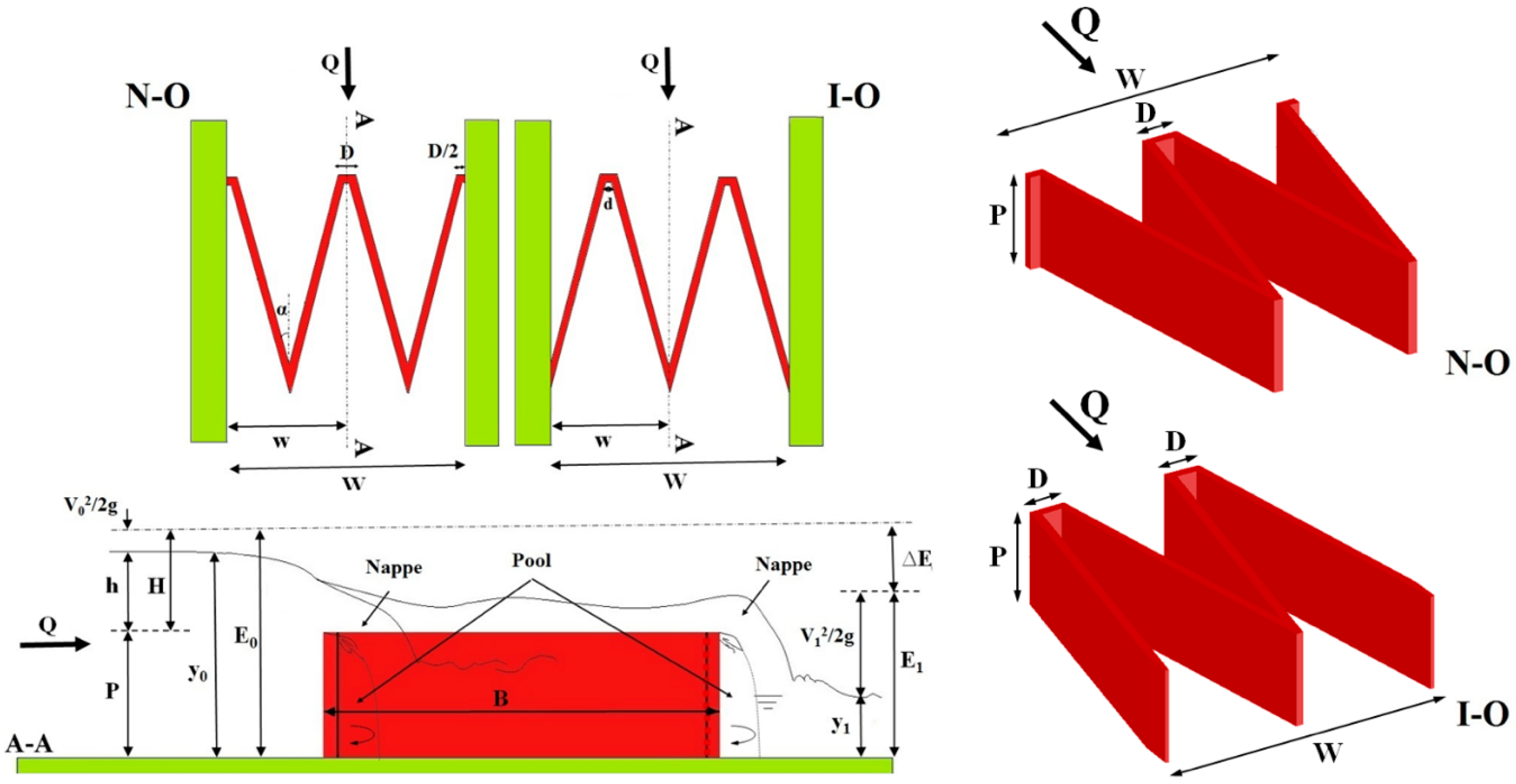
According to Figure 1, the main parameters affecting the discharge coefficient of the TTLW are (Equation (2)): the weir height (P), the number of labyrinth weir cycles (N), the length of each weir cycle (l), the width of each cycle (w), the weir external span (D), the weir internal span (d), the angle of the labyrinth weir wall (α), and the longitudinal slope of the weir bed (S₀).

$$Q=f(H,P,l,N,w,d,\alpha ,S_0,g)$$

(2)

After performing the dimensional analysis, Equation (2) can be written as follows:

$$f(\frac{Q}{L\sqrt{g}{H}^{1.5}},\frac{H}{P},\frac{w}{P},\frac{l}{P},N,\alpha ,S_0)=0$$

(3)

In test cases of our work where N = 2 and S₀ = 0, it follows that these parameters can be eliminated from Equation (3):

$$\frac{Q}{L\sqrt{g}{H}^{1.5}}=f(\frac{H}{P},\frac{w}{P},\frac{l}{P},\alpha )$$

(4)

Combining Equations (1) and (4) it is possible to derive the following equation:

$$C_d=f(\frac{H}{P},\frac{w}{P},\frac{l}{P}\alpha )$$

(5)

The effect of the dimensionless parameters presented in Equation (5) on the TTLW discharge coefficient will be examined in the next sections.

2.2. Effective Parameters in the Energy Dissipation

The energy dissipation rate in the TTLW can be investigated by comparing the total energy dissipation in the labyrinth weir (ΔE) with the maximum possible energy dissipation (ΔE_max). According to the special energy curve, as known, the minimum specific energy (E_min) occurs in critical flow conditions (Froude number (Fr) = 1). Thus, the minimum amount of energy remaining downstream of the TTLW will be as follows:

$$E_{1\min }=E_{\min }=1.5y_c$$

(6)

where y_c indicates the critical depth of passing flow the labyrinth weir. The maximum possible energy dissipation is therefore given by:

$$\mathsf{\Delta }{E}_{\max }=E_0-E_1{}_{\min }=E_0-1.5y_c$$

(7)

The equation of maximum relative energy dissipation is given as follows:

$$\frac{\mathsf{\Delta }{E}_{\max }}{E_0}=1-1.5\frac{y_c}{E_0}$$

(8)

The relative energy dissipation on the weir can be derived, through a dimensional analysis, based on the relationship of the geometric parameters of the weir and the flow conditions [30,31]. Regardless of the effect of viscosity and surface tension, the labyrinth weir energy dissipation can be stated as follows:

$$f(\mathsf{\Delta }E,E_0,y_c,P,l,w,\alpha )=0$$

(9)

Using Buckingham $\mathsf{\pi }$ theorem, the dimensionless parameters affecting the rate of energy dissipation over the TTLW wrote as follows:

$$\frac{\mathsf{\Delta }E}{E_0}=f(\frac{y_c}{E_0},\frac{l}{w},\frac{l}{P},\frac{w}{P},\alpha )$$

(10)

2.3. Numerical Model

FLOW-3D^® software package was used to numerically simulate the flow pattern. The software solves the three-dimensional Reynolds averaged Navier–Stokes equations (RANS) with the finite volume method [32,33]:

$$V_F\frac{\partial \rho }{\partial t}+\frac{\partial \left(\rho u{A}_x\right)}{\partial x}+\frac{\partial \left(\rho v{A}_y\right)}{\partial y}+\frac{\partial \left(\rho w{A}_z\right)}{\partial z}=R_{SOR}+R_{DIF}$$

(11)

$$\frac{\partial u}{\partial t}+\frac{1}{V_F}\left(u{A}_x\frac{\partial u}{\partial x}+v{A}_y\frac{\partial u}{\partial y}+w{A}_z\frac{\partial u}{\partial z}\right)=-\frac{1}{\rho }\frac{\partial P}{\partial x}+G_x+f_x$$

(12)

$$\frac{\partial v}{\partial t}+\frac{1}{V_F}\left(u{A}_x\frac{\partial v}{\partial x}+v{A}_y\frac{\partial v}{\partial y}+w{A}_z\frac{\partial v}{\partial z}\right)=-\frac{1}{\rho }\frac{\partial P}{\partial y}+G_y+f_y$$

(13)

$$\frac{\partial w}{\partial t}+\frac{1}{V_F}\left(u{A}_x\frac{\partial w}{\partial x}+v{A}_y\frac{\partial w}{\partial y}+w{A}_z\frac{\partial w}{\partial z}\right)=-\frac{1}{\rho }\frac{\partial P}{\partial z}+G_z+f_z$$

(14)

where (x, y, z) are the cartesian coordinates, P is the pressure, V_f is the volume fraction of the fluid in each cell, and (u, v, w) are the Cartesian velocity components. The A symbols are the fractional areas associated with the flow direction. The G terms are local accelerations of the fluid and the f terms are related to frictional forces. The ρ symbol indicates the fluid density, R_DIF is a turbulent diffusion term, and R_SOR is mass source.

A turbulence model is necessary to account for the turbulent Reynolds stresses. Here, the Renormalization Group (RNG) k-ε turbulence model was selected. This model has been applied to similar flow scenarios and is capable of providing accurate and efficient solutions [34,35,36,37,38]. The RNG k-ε model equations are given by:

$$\frac{\partial }{\partial t}(\rho k)+\frac{\partial (\rho k{u}_i)}{\partial x_i}=\frac{\partial }{\partial x_j}({\alpha }_k{\mu }_{eff}\frac{\partial k}{\partial x_j})+G_k+G_b-\rho \epsilon -Y_M+S_k$$

(15)

$$\frac{\partial }{\partial t}(\rho \epsilon )+\frac{\partial (\rho \epsilon u_i)}{\partial x_i}=\frac{\partial }{\partial x_j}({\alpha }_s{\mu }_{eff}\frac{\partial k}{\partial x})+C_{1s}-\frac{\epsilon }{k}(G_k+G_{3s}{G}_b)+C_{2\epsilon }\rho \frac{{\epsilon }^2}{k}-R_{\epsilon }+S_{\epsilon }$$

(16)

where k is the turbulent kinetic energy per unit mass, $\epsilon$ is the turbulence dissipation rate per unit mass, G_k is the production of turbulent kinetic energy due to velocity gradient, G_b is turbulent kinetic energy production from buoyancy, and Y_M is turbulence dilation oscillation distribution [39,40]. In the above equations, ${\alpha }_k$ = ${\alpha }_s$ = 1.39, C_1s = 1.42, and $C_{2\epsilon }$ = 1.6 are model constants. All of the constants are derived explicitly in the RNG procedure. The terms S_k and $S_{\epsilon }$ are source terms for k and $\epsilon$, respectively. Also $\mu$_eff is the effective viscosity (μ_eff = μ + μ_t), where μ_t is called eddy viscosity or turbulent viscosity. Among the two equation models, the one by Launder and Spalding [41] popularly known as RNG k-ε model, proposes:

$${\mu }_t=C_{\mu }\frac{\rho k^2}{\epsilon }$$

(17)

Here C_μ is an empirical constant equal to 0.09.

FLOW-3D^® uses an advanced algorithm for tracking free-surface flows, called the volume of fluid (VOF) [42]. The VOF method consists of three main components: fluid ratio function, VOF transport equation solution, and boundary conditions at the free surface. The VOF transport equation is expressed by (18):

$$\frac{\partial F}{\partial t}+\frac{1}{V_F}\left[\frac{\partial (F{A}_{x}u)}{\partial x}+\frac{\partial (F{A}_{y}v)}{\partial y}+\frac{\partial (F{A}_{z}w)}{\partial z}\right]=0$$

(18)

In the above equation, A is the average ratio of flow area along x, y, and z directions; u, v, and w are average velocities along x, y, z; and F is the fluid ratio function which takes on values between 0 and 1. If F = 0, the cell is completely full of air, and if F = 1, the cell is full of water. The free surface is tracked where F = 0.5.

3. Case Study

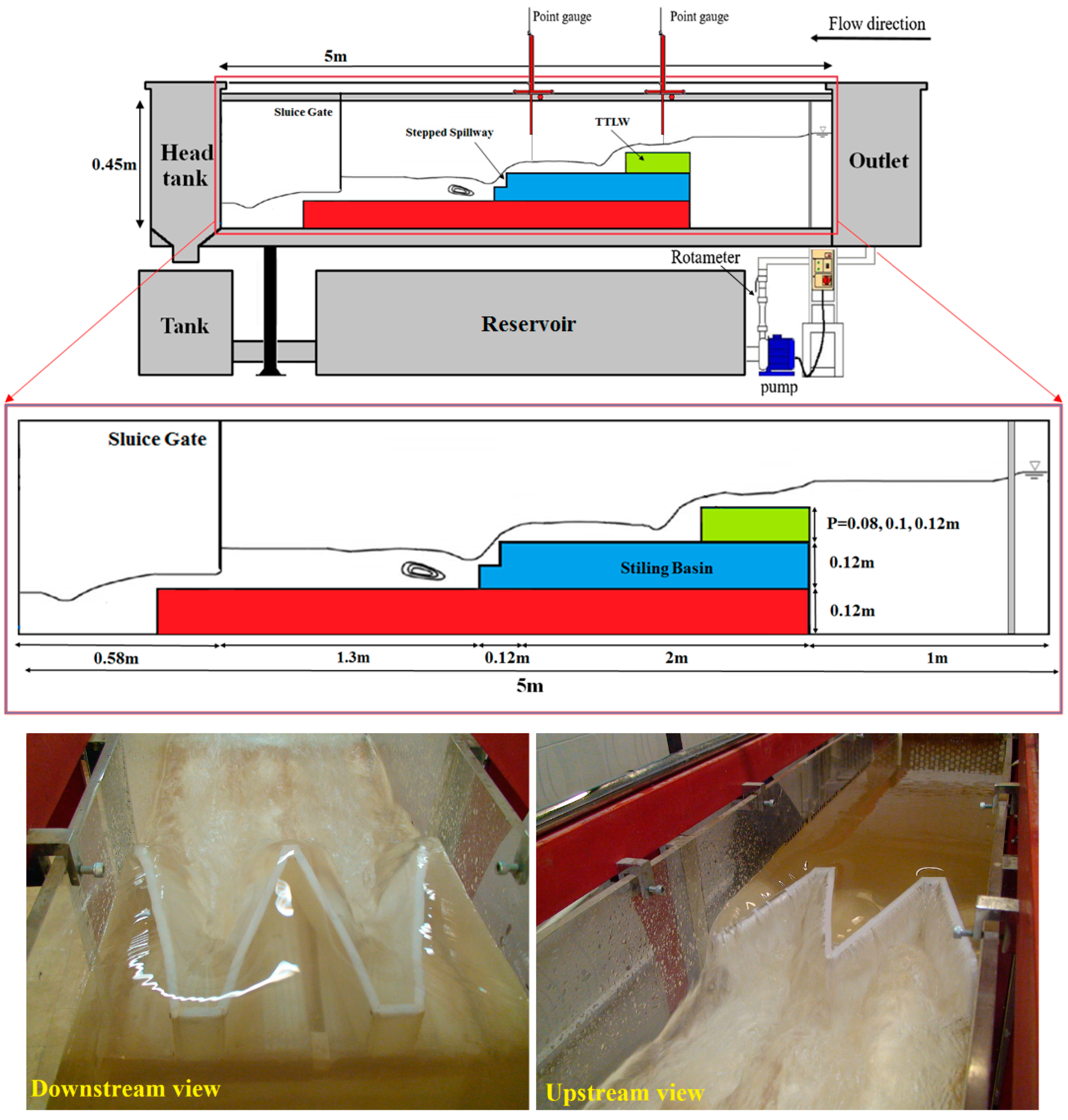
Laboratory tests were performed in a horizontal rectangular channel with length, width, and height of 5, 0.3, and 0.45 m, respectively. Ten weir models with heights of 0.08, 0.1, and 0.12 m were constructed (

Table 1. Geometrical properties of weir models and hydraulic flow parameters in the present study.

Models	Q (l/s)	α (°)	l (cm)	w (cm)	P (cm)	l/w	w/p	Fr0
Range	3–15	10–30	27–72	15	8–12	1.8–4.8	1.87–1.25	0.08–0.16

). To provide a smooth surface with the least roughness, floors and channel walls were constructed from Plexiglas. However, according to Johnson [43], the effect of channel walls on the discharge coefficient of labyrinth weir can be neglected. To ensure steady flow, weir models were installed 1.5 m downstream of the inlet tank. At the inlet of the channel, there was a screen that eliminated the flow turbulence and the flow slowly entered the laboratory flume. Channel flow was measured by two pumps each at a maximum discharge of 7.5 L/s by two valves connected to two rotameters with an accuracy of ±2% installed at the pump outlet (Figure 2). In total, 210 experiments were performed to investigate the research objectives.

The flow depth for both the upstream and downstream sections was determined by a gauge point mounted on the flume top with an accuracy of ±1 mm. This technique was adopted from previous studies, for example, Ghaderi et al. [44] and studies. To record the upstream flow depth, the gauge point was positioned at 3 h to 4 h [45]. Also, the flow depth was recorded downstream of the weir at a distance of 0.8 m. Upstream Froude number was calculated as Fr₀ = Q/[gW²(h + P)³]^0.5, downstream Froude number as Fr₁ = V₁/(gy₁)^0.5, Reynolds number as R = (gh³)^0.5/υ, critical depth as y_c = (Q²/Gw²)^1/3, upstream speed as V₀ = Q/y₀, and downstream speed as V₁ = Q/Wy₁.

Computational Mesh and Boundary Conditions

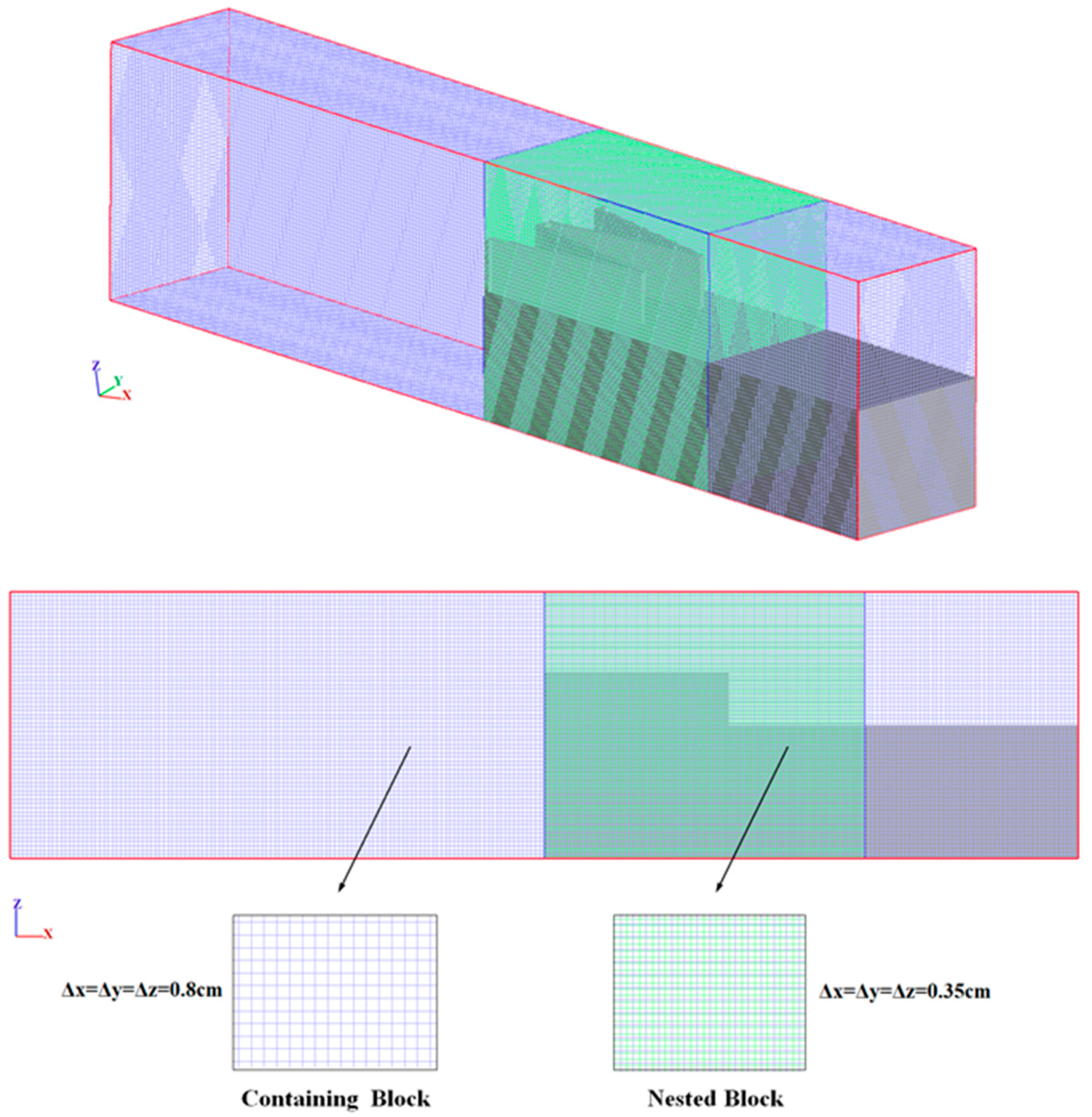
The weir setup was performed by inserting a sterolithography (STL) file. The spatial domain was meshed using a structured rectangular hexahedral mesh. A containing mesh block was created for the whole spatial domain, and then, a nested mesh block with refined cells for the area of interest (in correspondence of the weir) was built (see Figure 3). This technique, i.e., a nested mesh block, was adopted from previous studies (see, for example, Ghaderi and Abbasi [33], Choufu et al. [46], and Ghaderi et al. [47]). Considering the geometry dimensions, five computational meshes were tested to select the appropriate one. To this aim, a comparison between simulated and measured free surface profiles for the different meshes was performed (

Table 2. Mesh sensitivity analysis for the present study.

Test No.	Turbulence Model	Coarser Cells Size (cm)	Finer Cells Size (cm)	Total Mesh Number	Computational Time (min)	* MAPE (%) $100\times \frac{1}{\mathbf{n}}{\displaystyle \sum }_1^{\mathbf{n}}\left|\frac{{\mathbf{X}}_{\mathbf{exp}}-{\mathbf{X}}_{\mathbf{num}}}{{\mathbf{X}}_{\mathbf{exp}}}\right|$	** RMSE (cm) $\sqrt{\frac{1}{\mathit{n}}{\displaystyle \sum }_1^{\mathbf{n}}{{(\mathbf{X}}_{\mathbf{exp}}-{\mathbf{X}}_{\mathbf{num}})}^2}$
T1	k-ε (RNG)	1.10	0.65	711,758	50	19.39	3.44
T2	k-ε (RNG)	1.00	0.55	1,302,587	85	11.12	1.96
T3	k-ε (RNG)	0.90	0.45	1,997,425	120	6.07	0.85
T4	k-ε (RNG)	0.80	0.35	2,703,458	175	3.75	0.56
T5	k-ε (RNG)	0.70	0.30	3,587,624	220	3.32	0.44

* mean absolute percentage error, ** root mean square error, Xexp: experimental value of X; Xnum: numerical value of X; and n: total number of data.

).

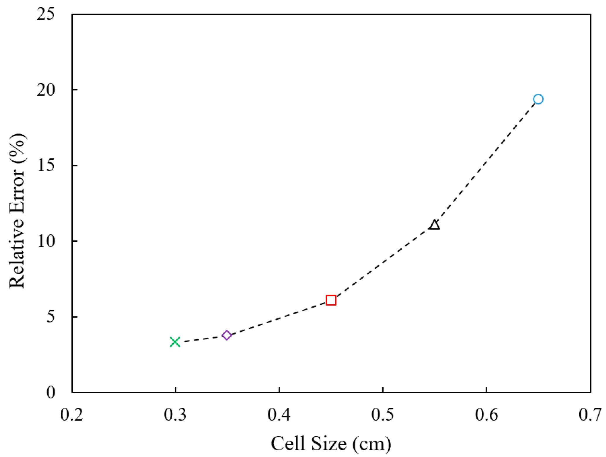
According to Figure 4, which shows the variation of the mean relative error as a function of the cell sizes for free surface profiles, we can see that the simulated free surface profiles exhibit better agreement with the measured free surface profiles for the finer cell size of 0.30 cm. In addition, the variation of mean relative errors can be neglected by decreasing the cell size from 0.35 cm to 0.30 cm. In summary, the cell size of 0.35 cm was selected and there were 598,500 coarse cells (0.8 cm in all directions) and 2,104,958 finer cells (0.35 cm in all directions). To reduce the effect of computational mesh on simulation results, the same mesh was adopted for all models of this research.

Computations in the viscous sub-layer were prevented. The first node was located near a wall in order to keep the dimensionless parameter of y⁺ (Equation (19)) in the range of 5 < y⁺ < 30 [48]. The ratio of turbulent and laminar influences in a cell, y⁺, is defined as:

$$y^{+}=\frac{y_p{u}_{*}}{\upsilon }$$

(19)

where y_p is the distance of the first node from the wall, u* is the shear velocity of the wall and υ is the kinematic viscosity.

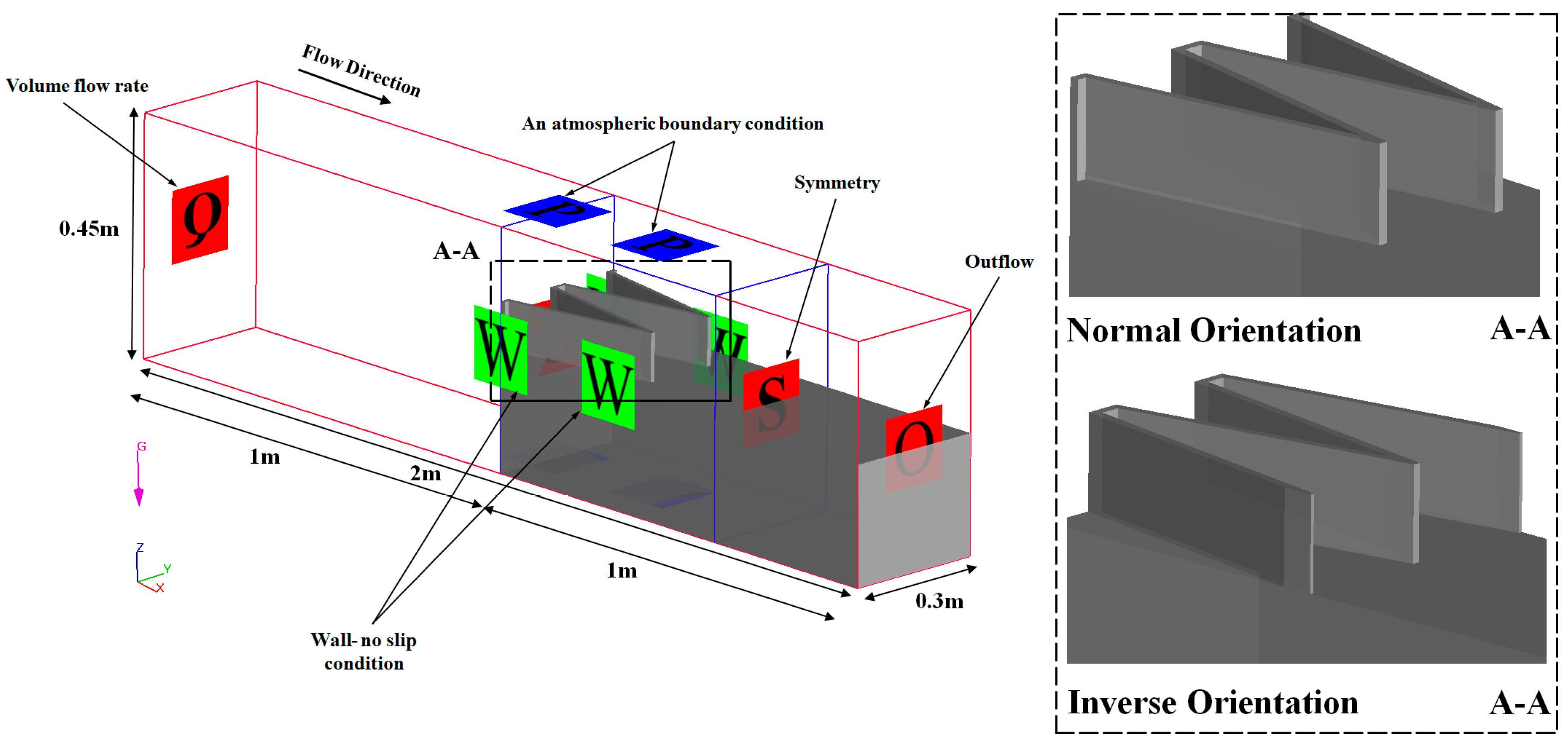
According to the experimental conditions, the inlet boundary condition was set to a discharge flow rate (Q; equal to the experimental flow exit discharge) and outlet (O) flow conditions were applied to the downstream boundary. Wall roughness has been neglected due to the small roughness of the material of the experimental facility (plexiglass) used for validation. The lower Z (Z_min) and both of the side boundaries were treated as rigid walls (W). No-slip conditions were applied at the wall boundaries, treated as non-penetrative boundaries. An atmospheric boundary condition was set to the upper boundary of the channel: the flow can enter and leave the domain as null von Neumann conditions are imposed on all variables, except for pressure, set to zero (i.e., atmospheric pressure). Symmetry boundary conditions (S) were used at the inner boundaries as well. Figure 5 shows the computational domain of the present study and the associated boundary conditions.

4. Results and Discussions

4.1. The Validity of the FLOW-3D Model

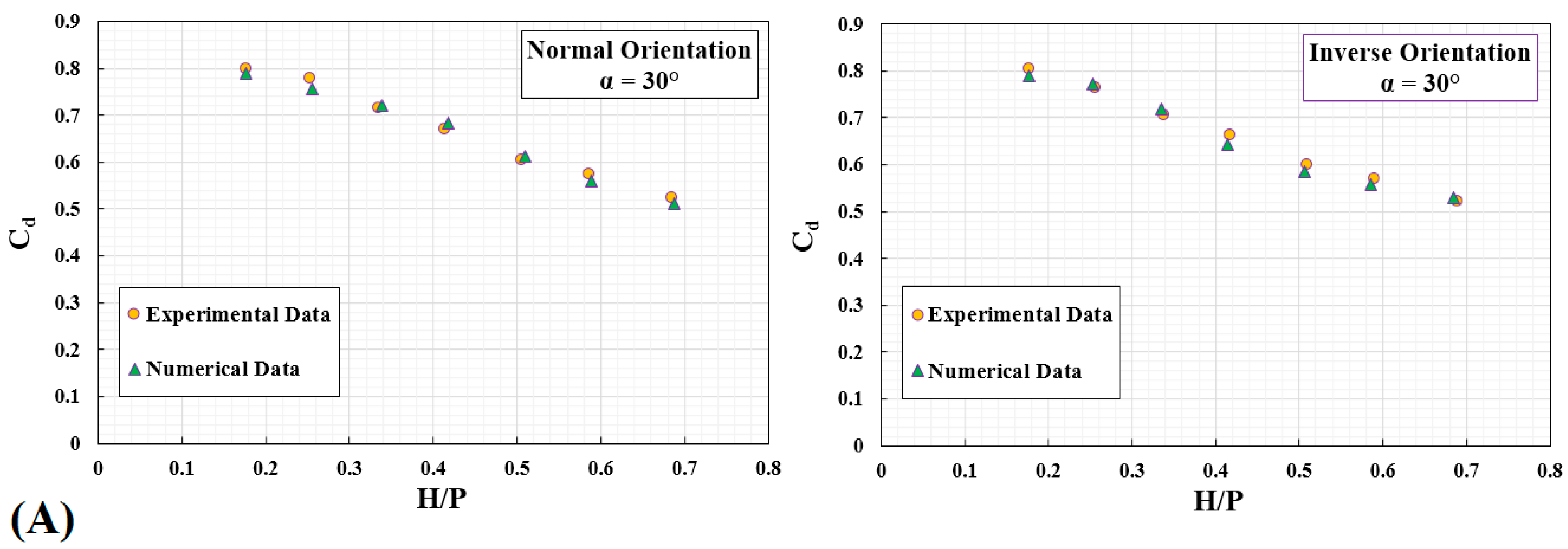
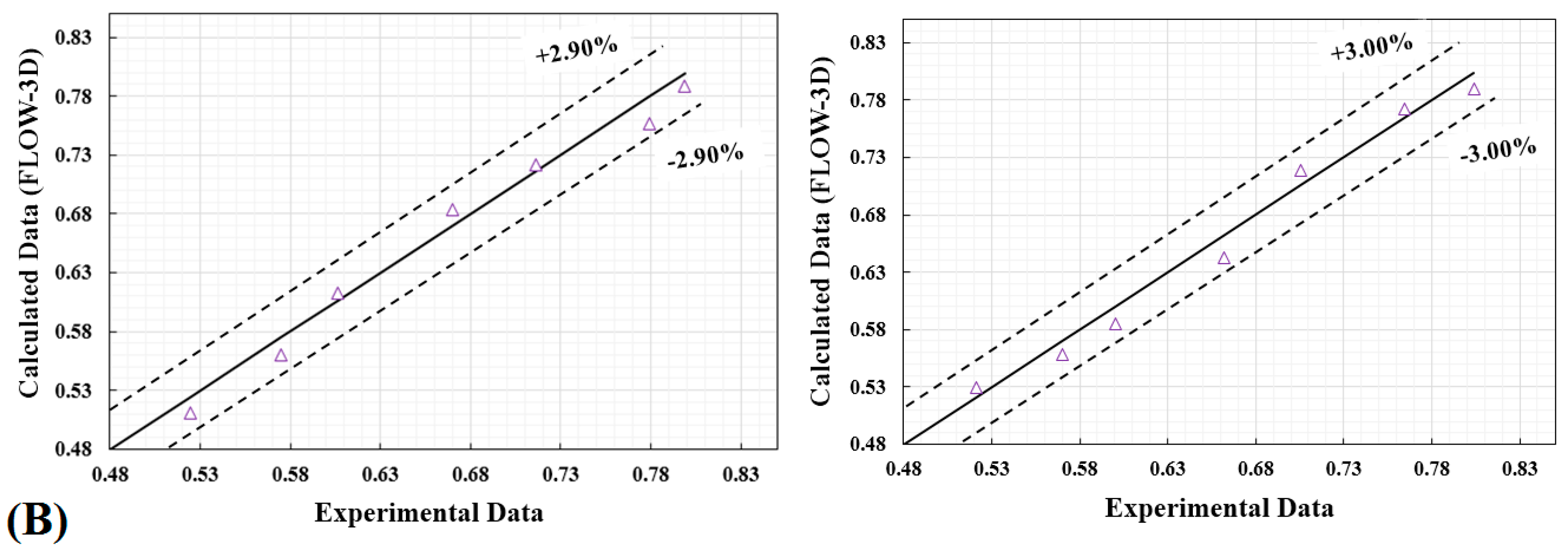
During the iteration, the time-step size has been controlled by stability (based on Courant number) and convergence criterion, which leads to time steps between 0.0001 and 0.0014 s. The evolution in time was used as a relaxation to the final steady state. The steady-state condition was checked for monitoring the kinetic energy of the flow, flow rate at the outlet boundary, and the free surface elevation at the inlet boundary. It was found that with the 12 s simulation of the flow, the solution became fully converged and the steady-state condition was achieved for all of the considered H/P (H: the hydraulic head, P: the weir height) values. The flow over the labyrinth weir in both orientations is simulated as a steady-state of flow (Figure 6A), and the discharge coefficient (C_d) is validated with experimental data. To ensure a good agreement between the numerical and experimental data, the error was determined and is presented in Figure 6B.

It can be observed that simulated discharge coefficient values at different H/P ratios were similar to the experimental data. Discharge coefficient C_d increased for a low H/P ratio and decreased for high ratios. A quantitative evaluation of the computed and measured discharge coefficient versus different H/P ratios comparisons were made by using mean absolute relative error (MARE).

$$MARE=\frac{1}{N}{\displaystyle \sum _{i=1}^N\left|\frac{O_i-P_i}{O_i}\right|}\times 100$$

(20)

where O_i and P_i are measured and computed values, respectively, and N is the total number of data.

Table 3. MARE Values for the discharge coefficient versus different H/P ratios on NO and IO orientation.

Model	H/P	Cd-NO-Measured Values	Cd-NO-Computed Values	Cd-IO-Measured Values	Cd-IO-Computed Values	MARE (%)-NO	MARE (%)-IO
Trapezoidal–Triangular Labyrinth Weir (TTLW)	0.176	0.799	0.789	0.804	0.790	1.29	1.70
	0.256	0.779	0.757	0.764	0.772	2.87	1.10
	0.338	0.716	0.722	0.706	0.719	0.77	1.90
	0.417	0.670	0.684	0.662	0.642	2.02	3.00
	0.509	0.606	0.613	0.600	0.585	1.14	2.50
	0.589	0.575	0.560	0.570	0.559	2.55	2.00
	0.688	0.525	0.510	0.521	0.529	2.72	1.60
	Mean					1.91	1.97

gives the results for MARE at different H/P ratio and weir orientation.

Regarding the overall mean value MARE in Table 3, there was a good agreement between numerical and laboratory results. The maximum percentage of error for H/P = 0.417 was 3% and the minimum value for H/P = 0.338 was 0.77%, which confirms the ability of the numerical model to predict specifications of flow over TTLW.

4.2. Hydraulics of Free Flow

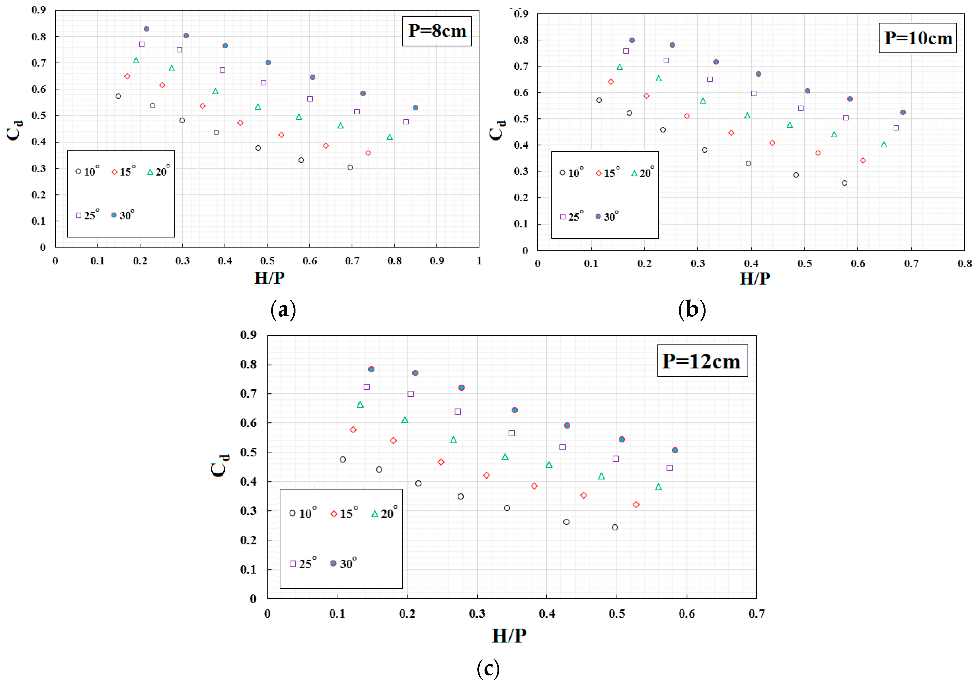
According to Ackers et al. [45] experimental investigations have demonstrated that the weir performance in free flow conditions can be assessed by the discharge coefficient. Figure 7 shows the variations of discharge coefficient C_d versus H/P for different weir geometries. It can be noted that C_d decreases by decreasing the sidewall angle due to the collision of the falling jets, for high value of H/P. It can be noted that for the low value of H/P, the C_d value is high, due to the fact that the collision of jets is not so severe. As a result, by increasing the sidewall angle, the decrease rate of C_d with H/P increases.

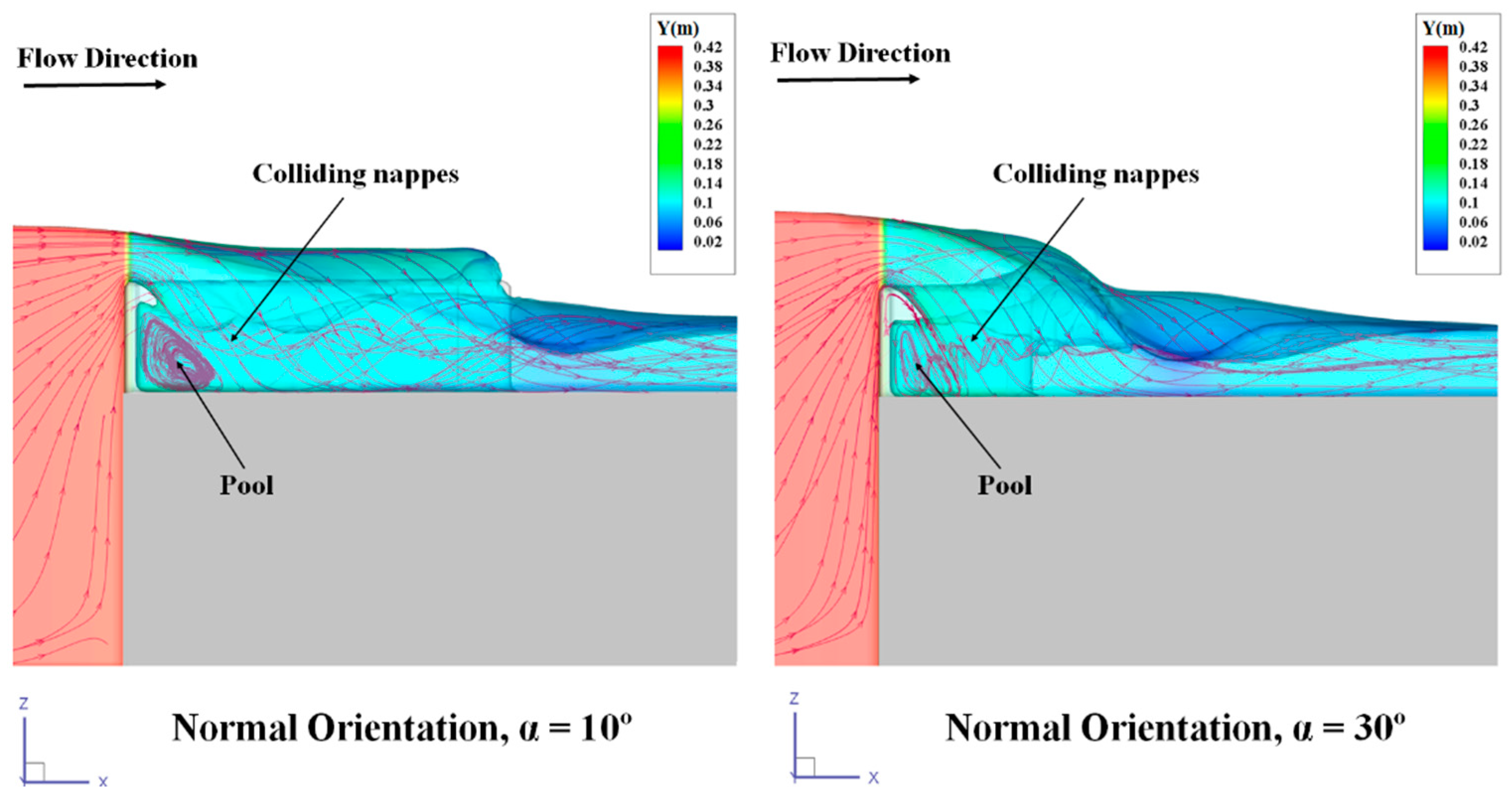
According to Crookston [49], nappe interaction occurs when two or more nappes collide. It can be seen that C_d decreases by increasing the weir heights due to nappe interaction. In fact, the nappe interaction increases with discharge, leading to a decrease in discharge coefficient C_d of the TTLW. For TTLW, nappe interference originates at the upstream apex and can produce wakes downstream of the apex (Figure 8). It can be stated that for triangular shape, downstream of the apex, nappe interactions do not happen.

The behavior of C_d with H/P for the weirs of different orientations, obtained from experimental and numerical results, is shown in Figure 9. It can be noted that the trend of discharge coefficient for normal and inverse orientation is the same and C_d decreases by decreasing the sidewall angle.

A comparison of experimental tests TTLW orientations showed that no difference in discharge efficiency was observed between the normal and inverse orientations (Figure 10).

4.3. Energy Charachterization and Flow Regime

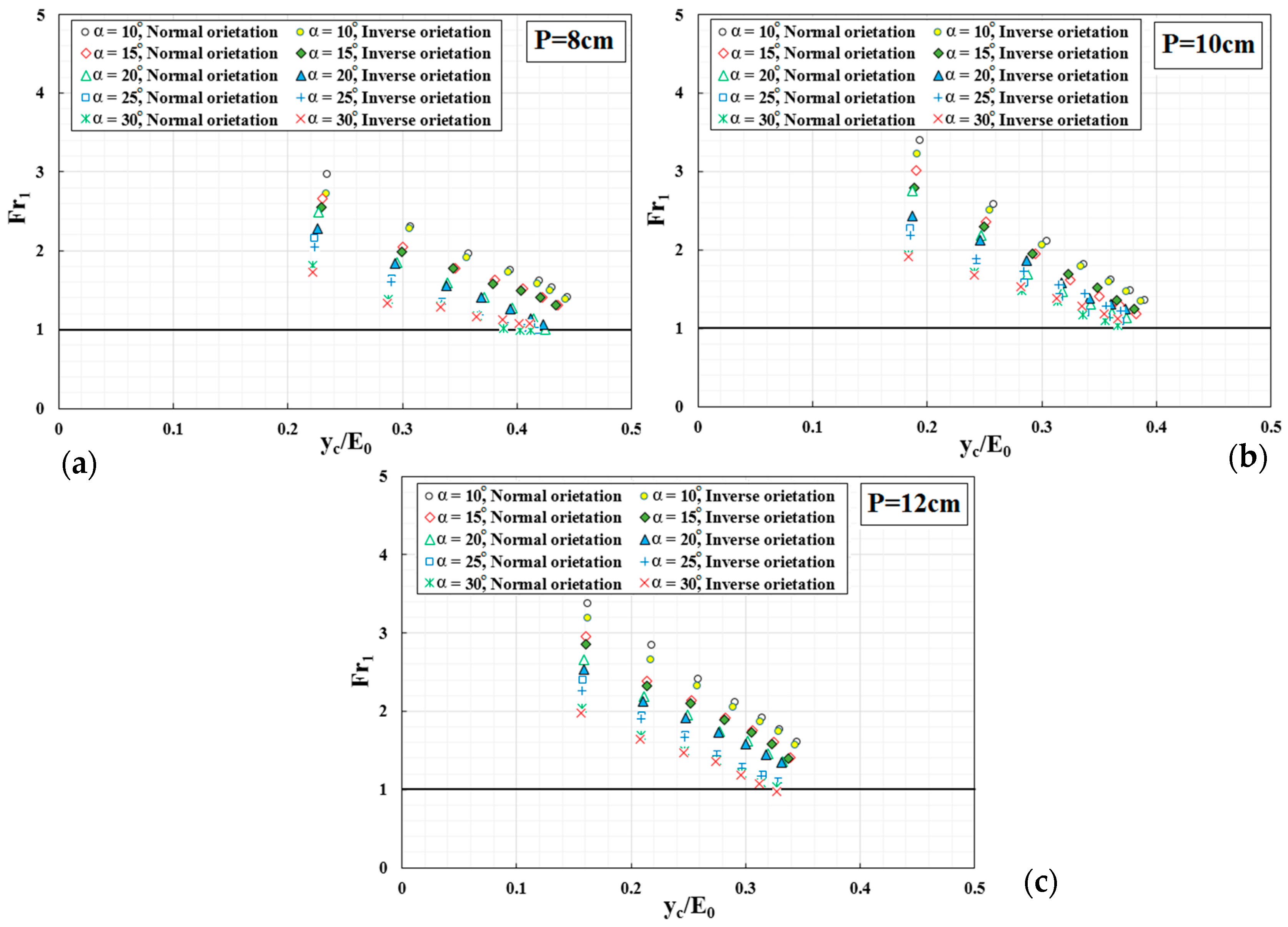
The weir downstream flow regime can be evaluated through the Froude number of flow Fr₁. Variation of Fr₁ with the relative critical depth y_c/E₀ for experimental results is shown in Figure 11 for different sidewall angles and height of the weirs. As highlighted in this figure, in most of the cases, the downstream flow regime of TTLW was supercritical: Froude number was larger than one with an increase of y_c/E₀ at different weir heights.

By increasing discharge (corresponding to the relative critical depth y_c/E₀), Fr₁ tends to be 1 but in some models with a high sidewall angle Fr₁ < 1 (subcritical flow); this is the result of weak hydraulic jump occurrence, due to circulating flows behind the nappes and collision of supercritical flows at the base of nappes (see Figure 12). Also, in the same discharge values, the submerged flow was earlier with a low sidewall angle.

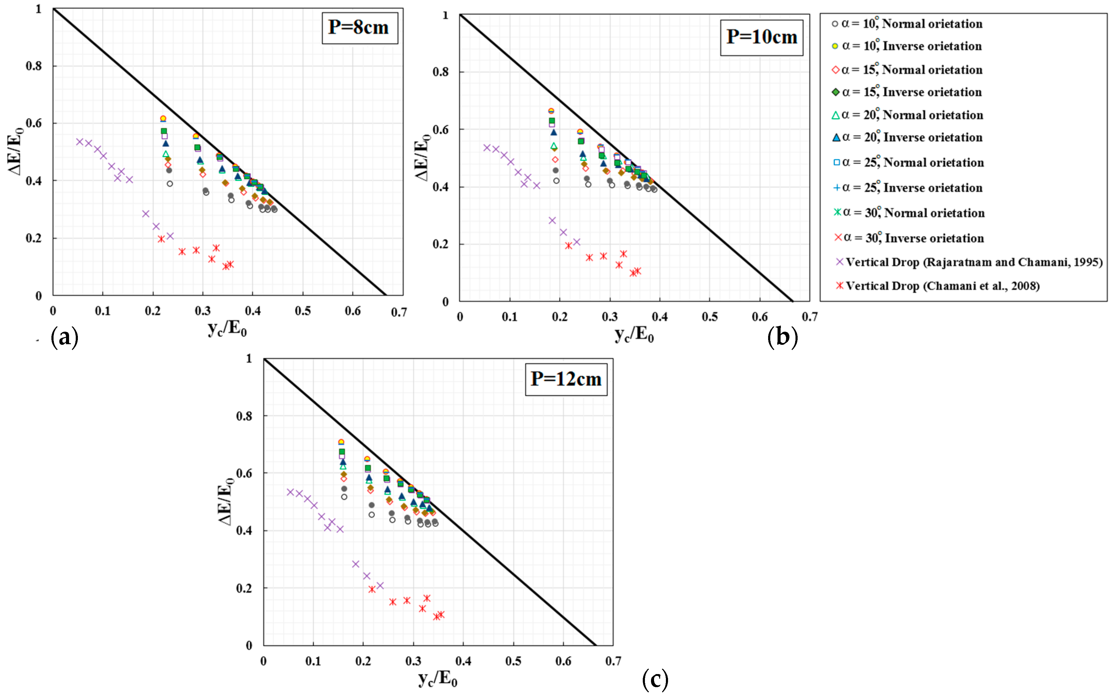
In Figure 13, the relative energy dissipation ∆E/E₀ versus the relative critical depth y_c/E₀ is presented. Energy dissipation results of vertical drops are compared with the results of Rajaratnam and Chamani [50] and Chamani et al. [51], indicating that TTLW approximately dissipates the maximum amount of energy. Increasing the sidewall angle and weir height (from 8 to 12) and subsequently increasing the dimensionless ratio of y_c/E₀, TTLW reduces more energy with respect to the vertical case. In fact, collision of nappes happens in the upstream apexes of TTLW, generating a localized hydraulic jump condition near it that leads therefore to energy dissipation. Moreover, with the creation of a pool behind the nappes in the upstream apexes of TTLW, circulating flow (in the pool) enhances the turbulent mixing and dissipates a large portion of energy (see Figure 12). It should also be noted that a weak hydraulic jump downstream of TTLW contributes to dissipating a higher and significant portion of energy.

For these reasons, values of energy dissipation on TTLW are more than energy dissipation on the vertical drop. Based on Rajaratnam and Chamani [50] and Chamani et al. [51], circulating flow in the pool is the main reason for energy dissipation on the linear weir and vertical drop.

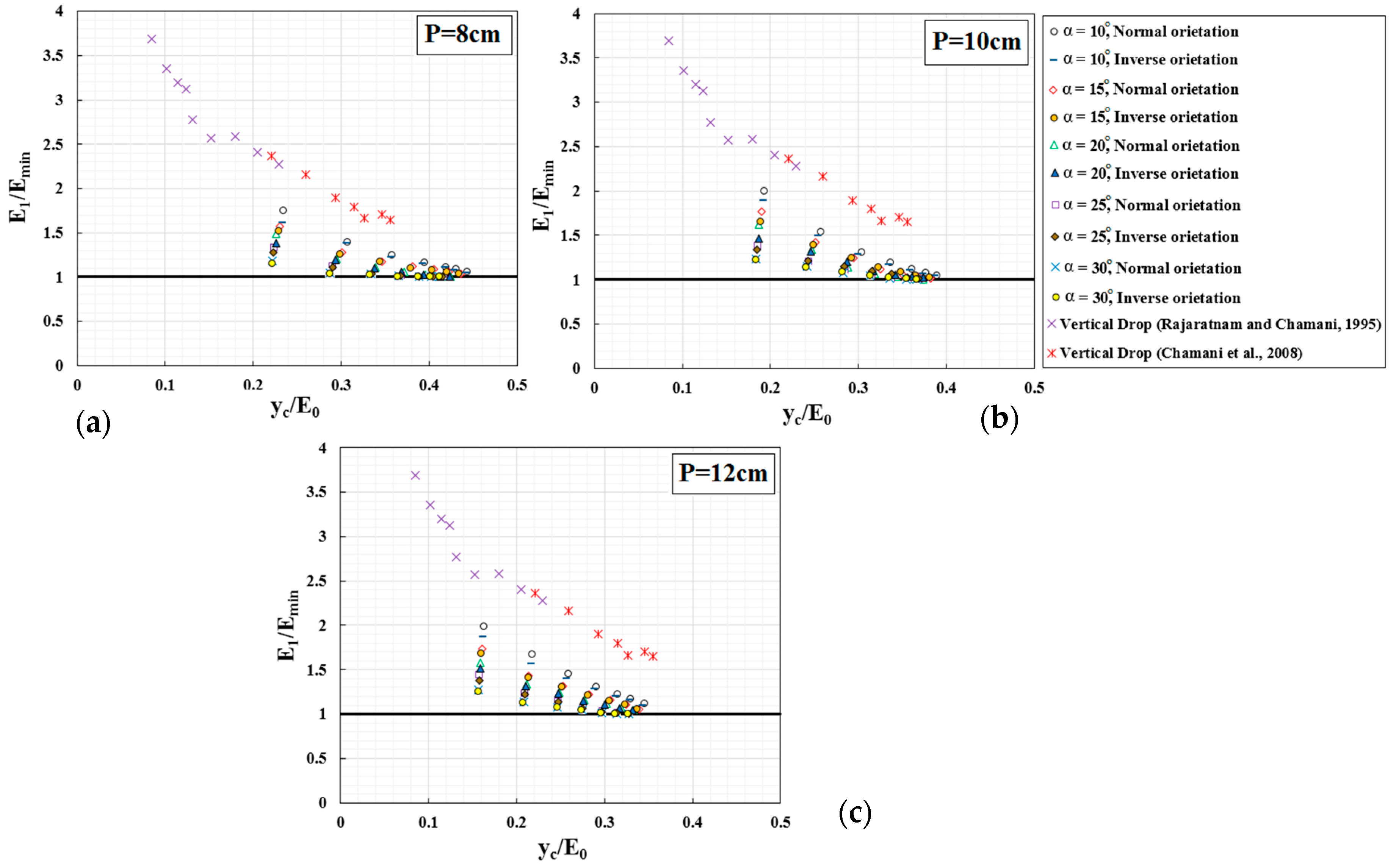
The measured residual energy E₁ downstream of weir models is normalized with the minimum theoretical minimum residual energy E_min, and results are then presented with the normalized critical depth y_c/E₀ (Figure 14). This result indicates that TTLW has energetic dissipation performance that leads to value of residual energy very close to the minimum possible value of residual energy. The energy dissipation of TTLW is largest compared to vertical drop and has the least possible value of residual energy as flow increases.

5. Conclusions

This paper presented and discussed the effects of the geometric parameters on the discharge coefficient, energy dissipation, and downstream flow regime of trapezoidal–triangular labyrinth weirs (TTLW) located in a reservoir with the normal and inverse orientations (experimentally and numerically studied).

In fact, weirs are very important structural measures extensively used, for instance, for water level and erosion control in rivers [52,53,54] and the optimization of their performance have objective advantages for hydraulic engineering works.

To simulate the free flow surface and turbulence, the volume of fluid (VOF) method and the RNG k-ε model in FLOW-3D software were used, respectively. The capability of this numerical method to reproduce the actual turbulent flow conditions in the analyzed flow over labyrinth weir has been assessed through comparisons with experimental data. The results of the study can be summarized as follows:

• It can be concluded that the FLOW-3D software can accurately predict characteristics of flow over TTLW. In comparisons between the calculated and measured free surface profiles, appropriate mesh with 2,118,270 elements by relative error and RMSE of 3.05%, 0.43 cm and maximum aspect ratio 1.07, was selected for calculations. The maximum and minimum value MARE errors are 3% and 0.77%.
• In the high value of H/P due to the collision of the falling jets, the discharge coefficient decreases by decreasing the sidewall. While for the low of H/P, the collision of jets is not so severe, hence in high values for C_d. Also, by increasing the sidewall angle, the decrease of C_d with H/P increases. Increasing the weir heights decreases the discharge coefficient due to nappe interactions occurring when two or more nappes collide, and the nappe interaction increases as discharge increases.
• In low discharge, hydraulics of flow over the TTLW has free flow conditions and for high discharge it has submerged conditions. In all models, the downstream Froude number is larger than one with an increase of relative critical depth y_c/E₀ at different weir heights.
• TTLW approximately dissipates the maximum amount of energy and increases the sidewall angle, weir height, and relative critical depth y_c/E₀, it reduces more energy dissipation. Circulating flows behind the nappes enhances the turbulent mixing and dissipates a large portion of energy in the upstream apexes of TTLW. It must be noted that a weak hydraulic jump downstream of TTLW contributes to the more energy dissipation.

Overall, CFD models may provide very good predictions of the energy dissipation and hydraulic characterization of flow over on labyrinth weirs for a different geometric and hydraulic conditions. These structures establish a unique, complex, and three-dimensional flow field in their vicinity. A hydraulic jump as the formation and location of hydraulic jump on the downstream of the weir can be simulated with numerical solutions. However, the accurate modeling of the erosion downstream of the weir caused by hydraulic jump, in particular in its vicinity, remains still an issue to be faced.

References

- Falvey, H. Hydraulic Design of Labyrinth Weirs; American Society of Civil Engineers: Reston, VA, USA, 2003. [Google Scholar]
- Mayer, P.G. Bartletts Ferry Project, Labyrinth Weir Model Studies; Project No. E-20-610; Georgia Institute of Technology: Atlanta, GA, USA, 1980. [Google Scholar]
- Houston, K.L. Hydraulic Model Study of the UTE Dam Labyrinth Spillway; Report No. GR-82-7; U.S. Bureau of Reclamations: Denver, CO, USA, 1982.
- Lux, F.; Hinchliff, D.L. Design and construction of labyrinth spillways. In Proceedings of the 15th Congress ICOLD, Lausanne, Switzerland, 24–28 June 1985; Volume 4, pp. 249–274. [Google Scholar]
- Lux, F. Design and application of labyrinth weirs. In Design of Hydraulic Structures 89; Alberson, M.L., Kia, R.A., Eds.; Balkema/Rotterdam/Brookfield: Toronto, ON, Canada, 1989. [Google Scholar]
- Tullis, B.P.; Amanian, N.; Woldron, D. Design of labyrinth spillways. J. Hydraul. Eng. 1995, 121, 247–255. [Google Scholar] [CrossRef]
- Talor, G. The Performance of Labyrinth Weirs. Ph.D. Thesis, University of Nottingham, Nottingham, UK, 1968. [Google Scholar]
- Hay, N.; Taylor, G. Performance and design of labyrinth weirs, American Society of Civil Engineering. J. Hydraul. Eng. 1970, 96, 2337–2357. [Google Scholar]
- Kumar, S.; Ahmad, Z.; Mansoor, T. A new approach to improve the discharging capacity of sharp crested triangular plan form weirs. J. Flow Meas. Instrum. 2011, 22, 175–180. [Google Scholar] [CrossRef]
- Crookston, B.M.; Tullis, B.P. Arced Labyrinth Weirs. J. Hydraul. Eng. 2012, 138, 555–562. [Google Scholar] [CrossRef]
- Carollo, G.F.; Ferro, V.; Pampalone, V. Experimental Investigation of the Outflow Process over a Triangular Labyrinth-Weir. ASCE J. Irrig. Drain. Eng. 2012, 138, 73–79. [Google Scholar] [CrossRef]
- Bilhan, O.; Emiroglu, M.E.; Miller, C.J. Experimental Investigation of Discharge Capacity of Labyrinth Weirs with and without Nappe Breakers. World J. Mech. 2016, 6, 207–221. [Google Scholar] [CrossRef] [Green Version]
- Abbaspuor, B.; Haghiabi, A.H.; Maleki, A.; Poodeh, H.T. Experimental and numerical evaluation of discharge capacity of sharp-crested triangular plan form weirs. Int. J. Eng. Syst. Model. Simul. 2017, 9, 113–119. [Google Scholar] [CrossRef]
- Azimi, A.H.; Hakim, S.S. Hydraulics of flow over rectangular labyrinth weirs. Irrig. Sci. 2019, 37, 183–193. [Google Scholar] [CrossRef]
- Savage, B.M.; Crookston, B.M.; Paxson, G.S. Physical and numerical modeling of large headwater ratios for a 15 labyrinth spillway. J. Hydraul. Eng. 2016, 142, 04016046. [Google Scholar] [CrossRef]
- Daneshfaraz, R.; Joudi, A.R.; Ghahramanzadeh, A.; Ghaderi, A. Investigation of flow pressure distribution over a stepped spillway. Adv. Appl. Fluid Mech. 2016, 19, 811–822. [Google Scholar] [CrossRef]
- Ghaderi, A.; Daneshfaraz, R.; Dasineh, M. Evaluation and prediction of the scour depth of bridge foundations with HEC-RAS numerical model and empirical equations (Case Study: Bridge of Simineh Rood Miandoab, Iran). Eng. J. 2019, 23, 279–295. [Google Scholar] [CrossRef]
- Daneshfaraz, R.; Minaei, O.; Abraham, J.; Dadashi, S.; Ghaderi, A. 3-D Numerical simulation of water flow over a broad-crested weir with openings. ISH J. Hydraul. Eng. 2019, 25, 1–9. [Google Scholar] [CrossRef]
- Biscarini, C.; Di Francesco, S.; Ridolfi, E.; Manciola, P. On the Simulation of Floods in a Narrow Bending Valley: The Malpasset Dam Break Case Study. Water 2016, 8, 545. [Google Scholar] [CrossRef] [Green Version]
- Paxson, G.; Savage, B. Labyrinth Weirs: Comparison of Two Popular U.S.A Design Methods and Consideration of Non-Standard Approach Conditions and Geometries. In International Junior Researcher and Engineer Workshop on Hydraulic Structures; Report CH61/06, Div. of Civil Eng.; Matos, J., Chanson, H., Eds.; The University of Queensland: Brisbane, Australia, 2006. [Google Scholar]
- Daneshfaraz, R.; Ghahramanzadeh, A.; Ghaderi, A.; Joudi, A.R.; Abraham, J. Investigation of the Effect of Edge Shape on Characteristics of Flow under Vertical Gates. J. Am. Water Works Assoc. 2016, 108, 425–432. [Google Scholar] [CrossRef]
- Dabling, M.R.; Tullis, B.P. Modifying the downstream hydrograph with staged labyrinth weirs. J. Appl. Water Eng. Res. 2018, 6, 183–190. [Google Scholar] [CrossRef]
- Ghaderi, A.; Abbasi, S.; Abraham, J.; Azamathulla, H.M. Efficiency of Trapezoidal Labyrinth Shaped Stepped Spillways. Flow Meas. Instrum. 2020, 72, 101711. [Google Scholar] [CrossRef]
- Macián-Pérez, J.F.; García-Bartual, R.; Huber, B.; Bayon, A.; Vallés-Morán, F.J. Analysis of the Flow in a Typified USBR II Stilling Basin through a Numerical and Physical Modeling Approach. Water. 2020, 12, 227. [Google Scholar] [CrossRef] [Green Version]
- Sangsefidi, Y.; Mehraein, M.; Ghodsian, M. Numerical simulation of flow over labyrinth weirs. Sci. Iran. 2015, 22, 1779–1787. [Google Scholar]
- Shaghaghian, M.R.; Sharifi, M.T. Numerical modeling of sharp-crested triangular plan form weirs using FLUENT. Indian J. Sci. Technol. 2015, 8, 1–7. [Google Scholar] [CrossRef] [Green Version]
- Carrillo, J.M.; Matos, J.; Lopes, R. Numerical modeling of free and submerged labyrinth weir flow for a large sidewall angle. Environ. Fluid Mech. 2019, 20, 1–18. [Google Scholar] [CrossRef]
- Norouzi, R.; Daneshfaraz, R.; Ghaderi, A. Investigation of discharge coefficient of trapezoidal labyrinth weirs using artificial neural networks and support vector machines. Appl. Water Sci. 2019, 9, 148. [Google Scholar] [CrossRef]
- Shafiei, S.; Najarchi, M.; Shabanlou, S. A novel approach using CFD and neuro-fuzzy-firefly algorithm in predicting labyrinth weir discharge coefficient. J. Braz. Soc. Mech. Sci. Eng. 2020, 42, 44. [Google Scholar] [CrossRef]
- Haghiabi, A.H.; Azamathulla, H.M.; Parsaie, A. Prediction of head loss on cascade weir using ANN and SVM. ISH J. Hydraul. Eng. 2017, 23, 102–110. [Google Scholar] [CrossRef]
- Mohammadzadeh-Habili, J.; Heidarpour, M.; Samiee, S. Study of energy dissipation and downstream flow regime of labyrinth weirs. Iran. J. Sci. Technol. Trans. Civil Eng. 2018, 42, 111–119. [Google Scholar] [CrossRef]
- Flow Science Inc. FLOW-3D V 11.2 User’s Manual; Flow Science Inc.: Santa Fe, NM, USA, 2016. [Google Scholar]
- Ghaderi, A.; Abbasi, S. CFD simulation of local scouring around airfoil-shaped bridge piers with and without collar. Sādhanā 2019, 44, 216. [Google Scholar] [CrossRef] [Green Version]
- Daneshfaraz, R.; Ghaderi, A. Numerical Investigation of Inverse Curvature Ogee Spillway. Civil Eng. J. 2017, 3, 1146–1156. [Google Scholar] [CrossRef] [Green Version]
- Zahabi, H.; Torabi, M.; Alamatian, E.; Bahiraei, M.; Goodarzi, M. Effects of Geometry and Hydraulic Characteristics of Shallow Reservoirs on Sediment Entrapment. Water 2018, 10, 1725. [Google Scholar] [CrossRef] [Green Version]
- Sangsefidi, Y.; MacVicar, B.; Ghodsian, M.; Mehraein, M.; Torabi, M.; Savage, B.M. Evaluation of flow characteristics in labyrinth weirs using response surface methodology. Flow Meas. Instrum. 2019, 69, 101617. [Google Scholar] [CrossRef]
- Ghaderi, A.; Dasineh, M.; Abbasi, S.; Abraham, J. Investigation of trapezoidal sharp-crested side weir discharge coefficients under subcritical flow regimes using CFD. Appl. Water Sci. 2020, 10, 31. [Google Scholar] [CrossRef] [Green Version]
- Ghaderi, A.; Dasineh, M.; Daneshfaraz, R.; Abraham, J. Reply to the discussion on paper: 3-D numerical simulation of water flow over a broad-crested weir with openings. ISH J. Hydraul. Eng. 2019, 1–9. [Google Scholar] [CrossRef]
- Yakhot, V.; Orszag, S.A.; Thangam, S.; Gatski, T.B.; Speziale, C.G. Development of turbulence models for shear flows by a double expansion technique. Phys. Fluids A Fluid Dyn. 1992, 4, 1510–1520. [Google Scholar] [CrossRef] [Green Version]
- Chero, E.; Torabi, M.; Zahabi, H.; Ghafoorisadatieh, A.; Bina, K. Numerical analysis of the circular settling tank. Drink. Water Eng. Sci. 2019, 12, 39–44. [Google Scholar] [CrossRef] [Green Version]
- Launder, B.E.; Spalding, D.B. The numerical computation of turbulent flows. In Numerical Prediction of Flow, Heat Transfer, Turbulence and Combustion; Pergamon: Bergama, Turkey, 1983; pp. 96–116. [Google Scholar]
- Hirt, C.W.; Nichols, B.D. Volume of Fluid (VOF) method for the dynamics of free boundaries. J. Comput. Phys. 1981, 39, 201–225. [Google Scholar] [CrossRef]
- Johnson, M. Discharge Coefficient Scale Effects Analysis for Weirs. Ph.D. Thesis, Utah State University, Logan, UT, USA, 1996. [Google Scholar]
- Ghaderi, A.; Daneshfaraz, R.; Torabi, M.; Abraham, J.; Azamathulla, H.M. Experimental investigation on effective scouring parameters downstream from stepped spillways Water Supply. Water Supply 2020, in press. [Google Scholar] [CrossRef]
- Ackers, P.; White, W.R.; Perkins, J.A.; Harrison, A.J. Weirs and Flumes for Flow Measurements; Wiley: Chichester, UK, 1978; p. 327. [Google Scholar]
- Choufu, L.; Abbasi, S.; Pourshahbaz, H.; Taghvaei, P.; Tfwala, S. Investigation of flow, erosion, and sedimentation pattern around varied groynes under different hydraulic and geometric conditions: A numerical study. Water 2019, 11, 235. [Google Scholar] [CrossRef] [Green Version]
- Ghaderi, A.; Daneshfaraz, R.; Abbasi, S.; Abraham, J. Numerical analysis of the hydraulic characteristics of modified labyrinth weirs. Int. J. Energy Water Res. 2020, 1–12, in press. [Google Scholar] [CrossRef]
- Sicilian, J.M.; Hirt, C.W.; Harper, R.P. FLOW-3D. Computational Modeling Power for Scientists and Engineers; Report FSI-87-00-1; Flow Science: Los Alamos, NM, USA, 1987. [Google Scholar]
- Crookston, B.M. Labyrinth Weirs. Ph.D. Thesis, Utah State University, Logan, UT, USA, 2010. [Google Scholar]
- Rajaratnam, N.; Chamani, M.R. Energy loss at drops. J. Hydraul. Res. 1995, 33, 373–384. [Google Scholar] [CrossRef]
- Chamani, M.R.; Rajaratnam, N.; Beirami, M.K. Turbulent jet energy dissipation at vertical drops. J. Hydraul. Eng. 2008, 134, 1532–1535. [Google Scholar] [CrossRef]
- Ridolfi, E.; Di Francesco, S.; Pandolfo, C.; Berni, N.; Biscarini, C.; Manciola, P. Coping with extreme events: Effect of different reservoir operation strategies on flood inundation maps. Water 2019, 11, 982. [Google Scholar] [CrossRef] [Green Version]
- Manciola, P.; Di Francesco, S.; Biscarini, C. Flood Protection and Risk Management: The Case of Tescio River Basin; IAHS-AISH Publication: Capri, Italy, 2009; Volume 327, pp. 174–183. [Google Scholar]
- Di Francesco, S.; Biscarini, C.; Manciola, P. Characterization of a Flood Event through a Sediment Analysis: The Tescio River Case Study. Water 2016, 8, 308. [Google Scholar] [CrossRef] [Green Version]
Figure 1.
The effective parameters of the trapezoidal–triangular labyrinth weir (TTLW).
Figure 2.
Schematic view of the test section and flumes.
Figure 3.
Sketch of mesh setup.
Figure 4.
Variations of the relative error of the free surface profiles versus cell size.
Figure 5.
Applied boundary conditions.
Figure 6.
(A) Comparison of discharge coefficient obtained from numerical solution with experimental data; (B) Determination of error percentage.
Figure 7.
Experimental results obtained for the effects of weir geometry on variations of discharge coefficient Cd versus H/P, (a) P = 8 cm, (b) P = 10 cm, (c) P = 12 cm.
Figure 8.
The collision of nappes from adjacent sidewalls of TTLW in (A) normal orientation and (B) inverse orientation.
Figure 9.
Variations of discharge coefficient Cd with H/P in normal and inverse orientation.
Figure 10.
Comparison of experimental tests TTLW orientations in discharge coefficient (Cd).
Figure 11.
Downstream Froude number (Fr1) versus the relative critical depth yc/E0, (a) P = 8 cm, (b) P = 10 cm, (c) P = 12 cm.
Figure 12.
The collision of nappes and circulating flows in the pool at upstream apexes of the TTLW.
Figure 13.
Energy dissipation on TTLW with vertical drop and maximum energy dissipation [31] (∆E/E0 versus yc/E0), (a) P = 8 cm, (b) P = 10 cm, (c) P = 12 cm.
Figure 14.
Comparison of the residual energy downstream of TTLW with a vertical drop, and minimum residual energy (E1/Emin versus yc/E0), (a) P = 8 cm, (b) P = 10 cm, (c) P = 12 cm.