Non-Fickian Solute Transport in Rough-Walled Fractures: The Effect of Contact Area


1
MOE Key Laboratory of Soft Soils and Geoenvironmental Engineering, Zhejiang University, Hangzhou 310058, China
2
Center for Hypergravity Experimental and Interdisciplinary Research, Zhejiang University, Hangzhou 310058, China
3
School of Resource and Environmental Engineering, Wuhan University of Science and Technology, Wuhan 430081, China
*
Author to whom correspondence should be addressed.
Water 2020, 12(7), 2049; https://0-doi-org.brum.beds.ac.uk/10.3390/w12072049
Submission received: 9 June 2020
/
Revised: 14 July 2020
/
Accepted: 15 July 2020
/
Published: 18 July 2020
(This article belongs to the Section Hydrology)
Abstract
:The influence of contact area, caused by normal deformation, on fluid flow and solute transport through three-dimensional (3D) rock fractures is investigated. Fracture surfaces with different Hurst exponents (H) were generated numerically using the modified successive random addition (SRA) method. By applying deformations normal to the fracture surface (Δu), a series of fracture models with different aperture distributions and contact area ratios (c) were simulated. The results show that the contact area between the two fracture surfaces increases and more void spaces are reduced as deformation (Δu) increases. The streamlines in the rough-walled fractures show that the contact areas result in preferential flow paths and fingering type transport. The non-Fickian characteristics of the “early arrival” and “long tail” in all of the breakthrough curves (BTCs) for fractures with different deformation (Δu) and Hurst parameters (H) were determined. The solute concentration distribution index (CDI), which quantifies the uniformity of the concentration distribution within the fracture, decreases exponential as deformation (Δu) and/or contact area ratios (c) increase, indicating that increased contact area can result in a larger delay rate of mass exchange between the immobile zone around the contact areas and the main flow channel, thus, resulting in a longer time for the solute to fill the entire fracture. The BTCs were analyzed using the continuous time random walk (CTRW) inverse model. The inverse modeling results show that the dispersion exponent decreases from 1.92 to 0.81 as c increases and H decreases, suggesting that the increase in contact area and fracture surfaces enhance the magnitude of the non-Fickian transport.
1. Introduction
Fluid flow and solute transport in fractured rock masses play a critical role in many geoscience and geoengineering disciplines, including groundwater contamination and remediation, nuclear waste disposal, shales oil extraction, carbon capture and storage, and geothermal energy extraction [1,2,3,4,5,6,7]. In a natural rock, the fracture network consists of numerous single fractures. Therefore, in order to improve the understanding of the transport properties in fractured rock, fluid flow and solute transport in a single fracture, which is the fundamental element of a fracture network, should be studied.
Using numerical and theoretical models, laboratory and field experiments, many previous studies have shown that macroscopic solute transport through a single fracture is often non-Fickian [8,9,10,11,12,13,14] and is characterized by the “early arrival” and “long tail”. Specifically, the “early arrival” means that the arrival time of the dimensionless particle concentration equals 0.5 in the BTCs, which is earlier than that predicted by the Fickian transport model, while the “long tail” represents the longer residence time of particles in the fracture [15]. Therefore, predictability of the observed non-Fickian is essential for environmental and human health-related issues, such as radionuclide transport in the subsurface or water quality evolution in managed aquifer recharge systems [11], as it controls the early arrival and the long residence time of particles. It is well known that matrix diffusion can induce non-Fickian transport [16] and that it plays an important role in transport processes in fracture–matrix systems [1,10,17,18,19], but our interest in this study is in rock formations such as fractured granite, in which the role of matrix diffusion is relatively minor and can often be ignored [20].
Geologic fractures always experience significant overburden stress or large displacement. Recently, experiments and numerical modeling have shown that increasing the normal/shear deformation increases the fracture roughness and the fracture contact area, resulting in lower relative permeability values and an evolution of flow process [21,22,23,24]. For instance, Zhou et al. [25] and Chen et al. [26] conducted a series of laboratory tests on fluid flow in rough fractures with normal loading, and they found that the fracture aperture and fluid conductivity decreased notably with high normal stress. Zhou et al. [25] also proposed that the normal loading could result in fracture closure, brittle damage of surface asperities and an increase in the contact area, which leads to a tortuous flow paths in the fractures. The surface roughness statistics for the experimental samples show that the surface roughness is remarkably degraded after testing. Vogler et al. [27] carried out laboratory experiments and numerical simulations to understand the coupled hydro-mechanical processes of fluid flow in heterogeneous fractures, and found that a nonlinear fracture closure and fluid injection pressure increase with loading. Liu et al. [28] numerically study the effect of shear on the evolutions of geometric and hydraulic properties of 3D self-affine fractures. They found that as shear deformation increases, the streamlines in the fracture become tortuous bypassing the contacts, showing obvious channeling flow phenomenon because of a large number of contacts and the small mean aperture. While normal/shear deformation has been shown to fundamentally impact fluid flow through rough-walled fractures, studies of non-Fickian transport on the scale of individual fractures have only focused on the role of fracture roughness and non-linear flow, while only a few studies have investigated the effects of normal deformation on solute and/or contaminant transport processes in single rock fractures. Jeong et al. [29] numerically investigated the flow and transport properties in a rough fracture under effective normal stress conditions, showing that the flow paths offered to particles become isolated from main channels due to the contact areas increasing with effective normal stresses. Koyama et al. [30] carried out numerical simulations of particle transport in rock fractures with normal loading; their results show that the effect of normal stress on the particle transport is significant, and dispersion becomes larger with increasing normal stress. Zhao et al. [4] deduced an analytic solution to model the coupled stress–flow–transport processes along a single 2D fracture embedded in a porous rock matrix. In their study, they investigated the influence of fracture aperture closure on solute transport along the fracture and into the rock matrix under increasing normal deformation conditions. Their results indicate that the concentrations both along the fracture and within the rock matrix decrease with increasing normal deformation due to the smaller fluid velocity (or fracture aperture). Kang et al. [31] reported the emergence of non-Fickian transport through a 3D rough-walled fracture due to increasing normal deformation. Their study showed that a larger number of contact areas in the highly deformed fracture led to a heterogeneous flow dominated by preferential channels and stagnation zones, resulting in non-Fickian transport behavior. Zou et al. [10] performed a direct numerical simulation of fluid flow and solute transport in a 3D rough-walled fracture–matrix system with several contact areas induced by normal and shear deformation. They found that the low-velocity and low-concentration zones were mostly located around the contact areas, which resulted in the long tails of the solute spreading within the fracture. Nevertheless, to the authors’ knowledge, quantifying the relationships between the magnitude of the non-Fickian transport and the contact area ratio due to normal deformation has not been attempted in previous studies.
Based on the previous studies described above, in order to assess the significance of non-Fickian character of solute diffusion, quantitative transport parameters should be introduced. To accomplish this, several transport models have been developed, such as the fractional advection–dispersion equation (FADE), the mobile–immobile method (MIM), the multi-rate mass transfer model and the continuous time random walk (CTRW) model. A detailed description and comparison of these transport models can be found in several previous studies [6,9,32,33,34,35]. By fitting non-Fickian BTCs to the different transport models, it is possible to accurately estimate the transport parameters and quantitatively evaluate the non-Fickian transport. The CTRW model was shown to be capable of capturing both Fickian and non-Fickian transport, and the inverse CTRW model has been successfully applied to many applications for characterizing non-Fickian BTCs. For example, the non-Fickian BTCs in heterogeneous porous media and single variable-aperture fractures [9,36,37]. However, the capability of the CTRW model to capture the non-Fickian characteristics induced by the contact area in a 3D single fracture still needs to be investigated.
Here, we demonstrate that an increase in contact area caused by normal deformation can induce non-Fickian transport in fractures. Normal deformation (Δu) transforms the fracture’s geometry from a relatively homogeneous flow structure to a very heterogeneous flow structure. The contact area between the two fracture surfaces increases and more void spaces are reduced as the mean fracture aperture decreases, after which the flow becomes organized into preferential flow channels and stagnation zones. To study the impact of the contact area ratio (c) on the flow and transport, a self-affine fractal model is applied to generate rough-walled fractures with different surface roughness parameters (H) using the modified successive random addition (SRA) method. The evolutions of the aperture distribution in the deformed rough-walled fracture are simulated based on the topographical data for the generated fracture surfaces. Then, the flow and transport problem through deformed rough-walled fractures is solved. Then, the influence of the normal deformation and contact area ratio on the flow paths, permeability, and non-Fickian transport are estimated. The non-Fickian transport properties resulting from the different H, Δu, and/or c are systematically investigated. Our findings further our understanding of solute transport through fractured media by linking the magnitude of the non-Fickian transport behavior with the contact conditions in fractures.
2. Fracture Model
2.1. Fracture Generation
In geological formations, the surface roughness of natural rock fractures typically follows a self-affine fractal distribution [38,39,40,41,42,43], which can be commonly simulated using fractional Brownian motion (fBm). Several methods have been attempted in the previous study to employ fBm to generate fracture surfaces [44,45]. The most widely used methods are Fourier transformation, the randomization of the Weierstrass–Mandelbrot function, and SRA. In this study, the SRA algorithm is used to generate fracture surfaces for its efficiency and straightforwardness [9,46,47,48,49,50,51].
The fracture wall height can be simulated from a two-dimensional fBm (or 2D Wiener–Brownian stochastic process) as the realization of a random, continuous, single-valued function with . Then, the stationary increment, with , over the distance (lag) h = (hx2 + hy2)1/2 has a centered Gaussian distribution with variance σ2 [46,52]. The statistical self-affine property of the fBm increment can be expressed as
where 〈•〉 represents the mathematical expectation, H is the scaling parameter or the Hurst exponent varying from 0 to 1 and related to the 3D fractal dimension (D) by D = 3 − H (for the surface; D = 2 − H for the profile) [46,53], and r is a constant. The variance is defined as
Based on the scaling properties of fBm, a modified SRA algorithm was developed by Liu et al. [47] and Ye et al. [46] to generate the fracture surfaces, and it improves the poor scaling and correlation properties of the fractal distributions involved in the traditional SRA algorithms.
By using Liu’s algorithm, a series of self-affine surfaces were generated with different H values. It should be noted that the H of natural rock fractures has proved to vary mostly between 0.45 and 0.87 [40,51,54]. Therefore, H values equal to 0.50, 0.55, 0.60, and 0.65 were selected in this study for comparison. Limited by the computer power and its memory capacities of solving the Navier–Stokes equation and advection–diffusion equation for the 3D self-affine rough fracture models with highly fine representation of the fracture surfaces, a domain of the surface of 32 mm × 32 mm in size that consist of a 128 × 128 grid was obtained with an interval of 0.25 mm. The choice of the sample interval is reasonable to represent the geometrical features of fracture surfaces, as an interval range from 0.2 mm to 0.4 mm was commonly employed in research when using a high-resolution 3D laser scanning system to obtain the topographical data of rock sample surfaces [8,51,55]. A more detailed description for generating self-affine surfaces using the modified SRA method is described by Ye et al. [46].
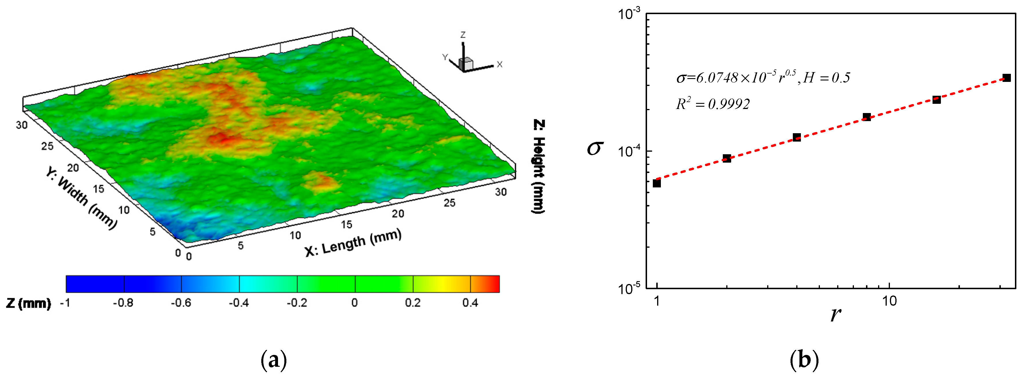
For generating the fBm distribution surface more accurately, we optimized the SRA method by controlling the error between the input roughness parameter H and the fitted H value of less than 0.001. Figure 1 shows a simulated example with H = 0.50 and an analysis of the scaling property. The calculation between the standard deviation (σ) and the lag (r) in the horizontal direction shows that the fitted H value is almost equal to the input values. It is further verified that the modified SRA algorithm is robust and is capable of generating fBm distributions accurately.
2.2. The Relationship between the Aperture Distribution, Contact Area Ratio, and Normal Deformation
Since the response of fluid flow and solute transport through a fractured medium is highly sensitive to fracture aperture, it is important to accurately simulate the variation in aperture during the shear and compression processes. Previous studies have shown that the aperture distributions of both natural and artificial fractures mostly exhibit truncated Gaussian distributions [56,57,58]. In this study, the method proposed by Wang et al. [59] was applied to generate the apertures with truncated Gaussian distributions.
Initially, the lower surface of the fracture is generated through the above modified SRA algorithm and is described using the function . Then, the upper surface is generated by replicating the lower surface and displacing it through shear deformation . It is expressed as , where is the mean aperture between the lower and upper surfaces in the initial state. Therefore, the aperture distribution can be calculated using
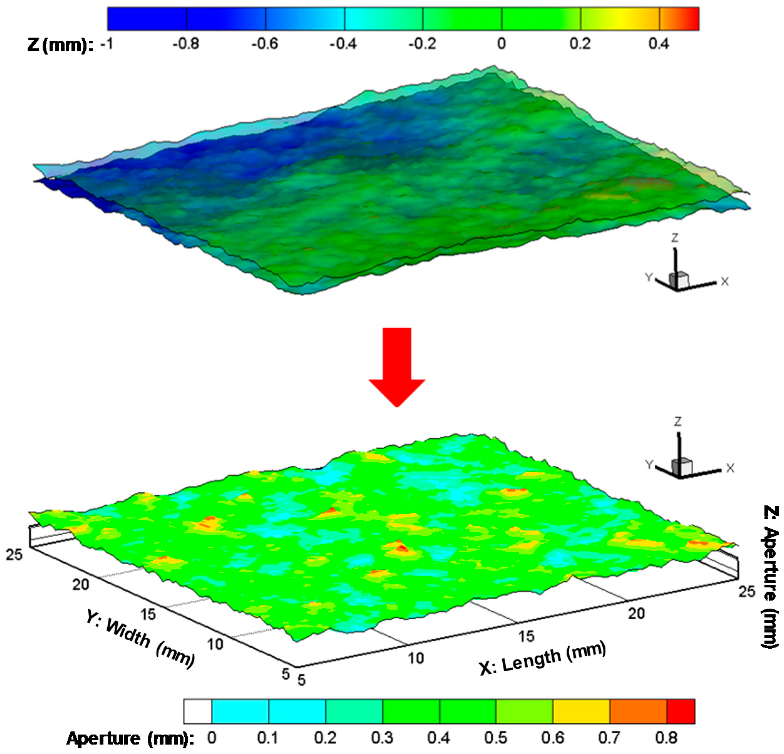
The value of indicates the contact point between the two fracture surfaces. A 20 mm × 20 mm aperture field was extracted from the central part of the original model to ensure a constant analysis area, due to the decreasing nominal contact area between the upper and lower fracture surfaces during shear deformation. Shear deformation was used in the generation of the fractures. An initial mean aperture of was adopted to ensure that the initial aperture distribution satisfied the Gaussian distribution. Figure 2 shows the original 3D self-affine fracture and the generated aperture distribution for H = 0.50.
When rough-walled fractures are subjected to normal deformation Δu, the two fracture walls shift vertically due to the normal stress. However, due to the heterogeneity in the micro-geometrical topography, the mechanism of fracture deformation is complex. For simplicity, the penetration model suggested by Oron and Berkowitz [60] and Walsh et al. [56] was adopted to characterize the deformation of the aperture distribution; a detailed explanation of the penetration model is described by Ye et al. [46]. Based on this model, the aperture distribution can be calculated using
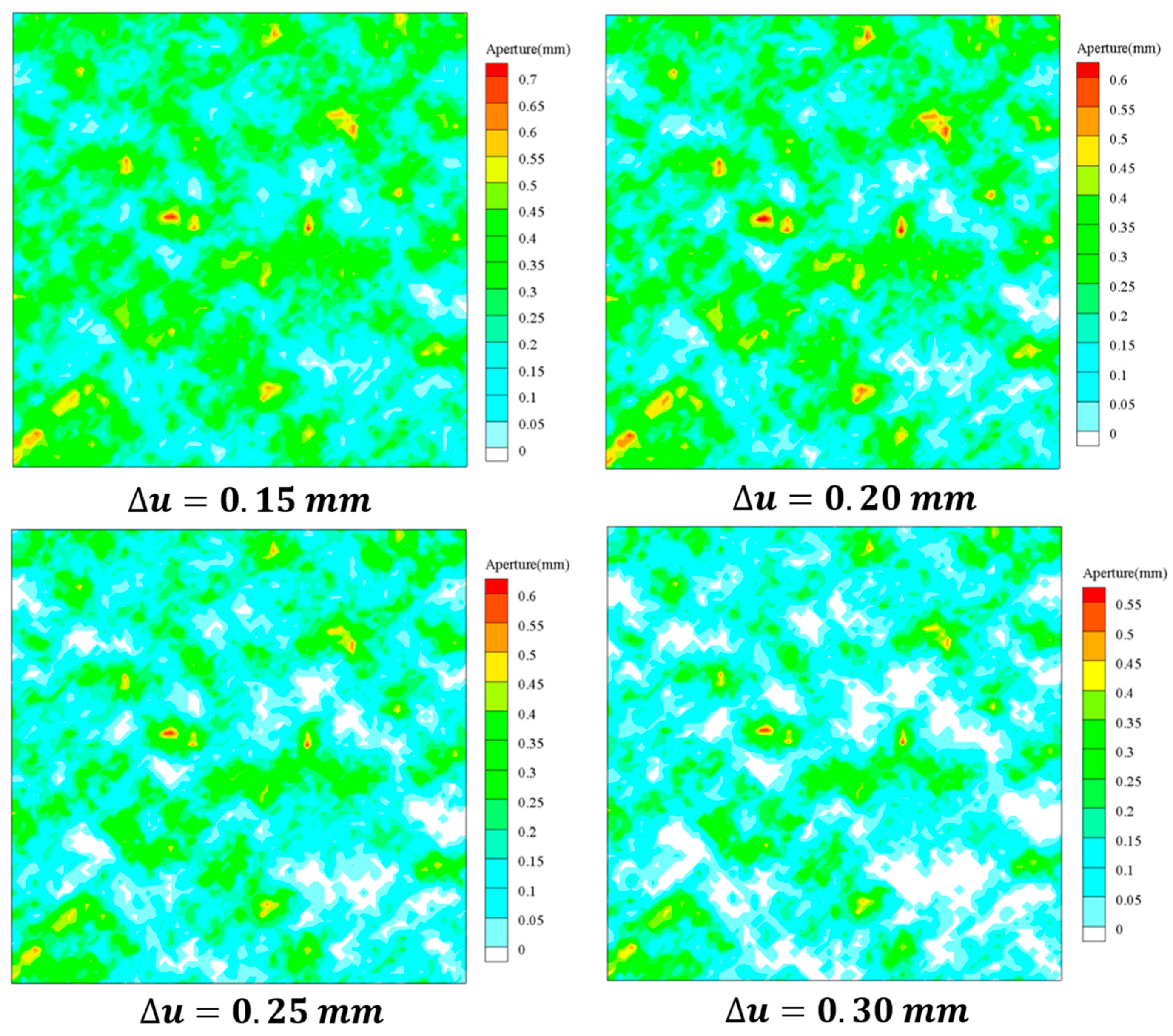
Figure 3 shows an example of the changes in the aperture distribution and contact area for different normal deformation conditions () for H = 0.50.
As can be seen in Figure 3, the size of the apertures decreases and the contact area increases as the normal deformation across the fractures increases. According to our previous study [46], the aperture distribution for b ≥ 0 can be described as a function of a mean value of u and a standard deviation of σ:
Thus, the frequency of the contact area with zero aperture value can be derived as:
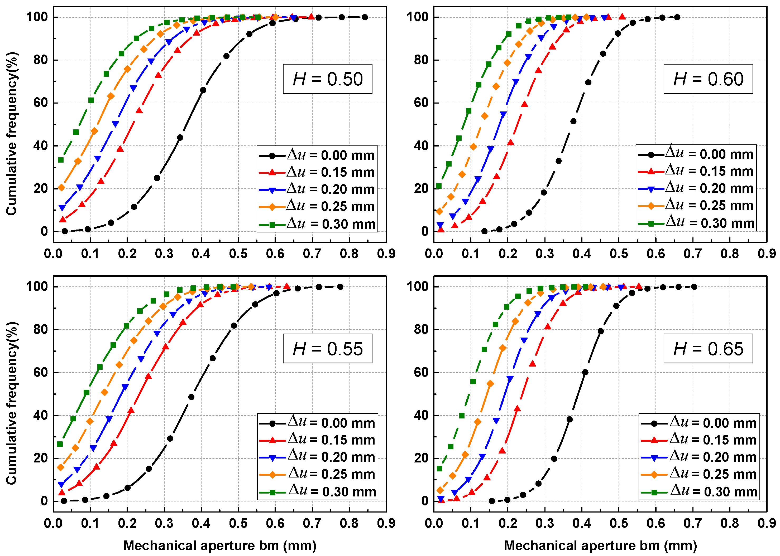
where erfc is a complementary error function. In this study, the contact area is considered to be zero between the two rough-walled fracture surfaces. Therefore, on account of aperture truncation, the cumulative probability distributions of fracture aperture for fractures with different ∆u and H are presented, as shown in Figure 4.
As shown in Figure 4, for the case of Δu = 0.00 mm, the cumulative probability distribution curves show a typical Gaussian distribution for different H. However, as Δu increases to 0.30 mm, the cumulative probability distribution curves shift to the left, and shows a truncated Gaussian distribution. For a certain H value, the frequency corresponding to b = 0 increases as Δu increases, indicating that the contact area between the two fracture surfaces increases, and more void spaces are reduced by the normal deformation. An increase in the H value has the opposite impact on the contact pattern and reduces the contact areas, and it can be found that the shape of the cumulative probability distribution curve changes from a sharp curve to a broader curve as H decreases. This is due to the fact that for H = 0.50, roughness spatial correlations are short, i.e., peaks are followed by valleys; when applying a normal deformation to the surface, peaks are clutched together, and contact area ratios increase with Δu. As H increases, peaks and valleys become wider, resulting in less contact areas clutched together under normal deformation, thus, the curve dependency between Δu and c decreases.
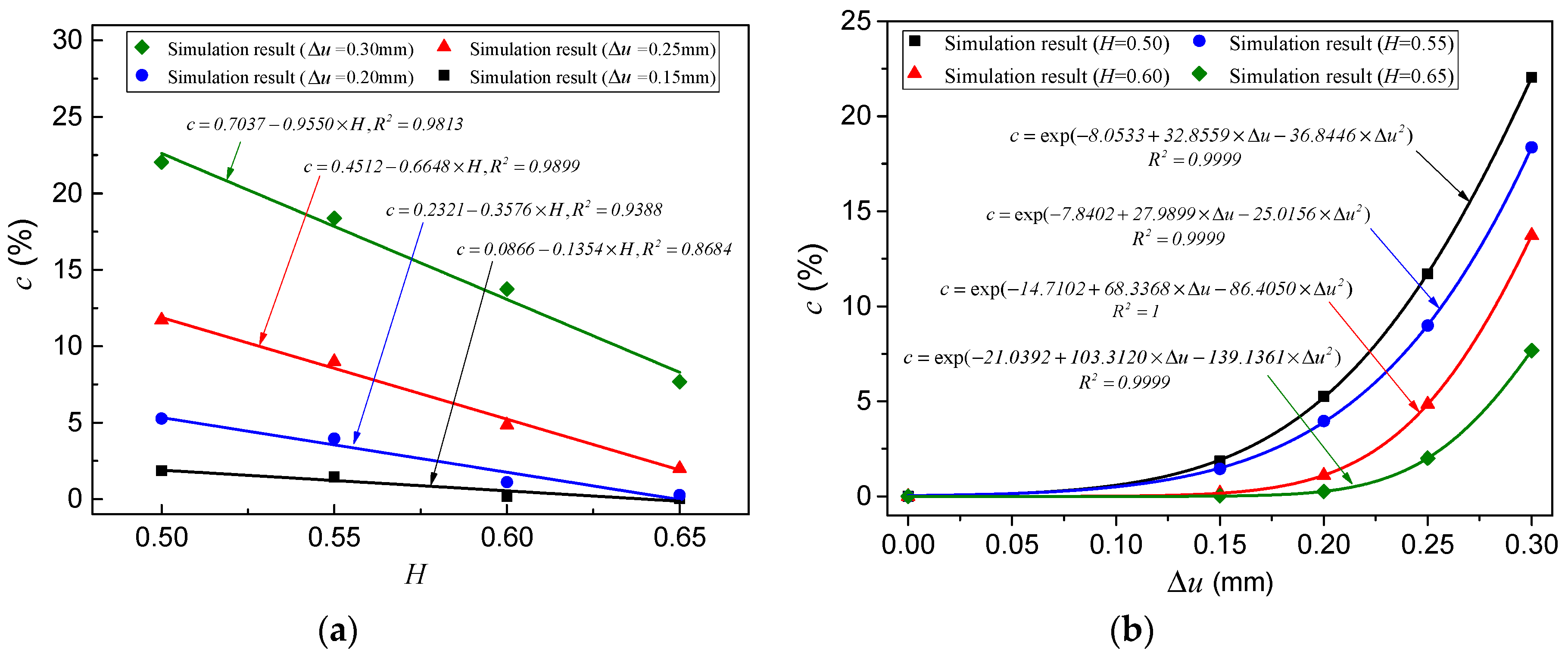
In this study, the locations where the apertures are equal to or less than zero represent the contact areas. The contact area ratio c (dimensionless) is proposed here to characterize the contact characteristics, which is defined as the ratio of the area of the contacts to the total area of the fracture:
where (M2) is the area of contacts, including dead voids, with no contribution to the flow; and (M2) is the total area of the fracture. Figure 5 shows the changes in c for different Δu and different H. The results show that c increases with increasing Δu, regardless of the value of H used. Figure 5 also shows that the growth rate of c at smaller H values (i.e., H = 0.5) is higher than that at larger H values (i.e., H = 0.65), directly indicating the important role of surface roughness in developing contact area under normal deformation conditions. This is due to the fact that for H = 0.50, roughness spatial correlations are short, i.e., peaks are followed by valleys; when applying a normal deformation to the surface, peaks are clutched together, and contact area ratios increase with Δu. As H increases, peaks and valleys become wider, resulting in less contact areas clutched together under normal deformation, thus, the curve dependency between Δu and c decreases.
3. Direct Simulation of Conservative Solute Transport
3.1. Physical Considerations and Governing Equations
The aperture distribution of natural rock fractures is variable and plays an important role in absorption and chemical reaction processes [1,10,18,19,61,62]. Bodin et al. [5,63] provided a comprehensive review of the key physical mechanisms involved in fracture–matrix systems, which mainly include solute advection, dispersion, and diffusion in the fracture; matrix diffusion from the fracture into the matrix; fracture surface and matrix sorption; decay; and chemical reactions. However, in this study, to highlight the variations with increasing normal deformation and contact area ratio, we only consider three major transport mechanisms for simplicity: the advection, dispersion and diffusion mechanisms within 3D self-affine fractures.
The fluid-flow field in a single rough-walled fracture can be solved directly using the Navier–Stokes and continuity equations, which describe isothermal, incompressible, and homogenous single Newtonian steady flow:
where , , , and are the fluid density (kg/m3), velocity vector (m/s), total pressure (Pa), and dynamic viscosity (Pa s), respectively. For the numerical simulations, the fracture surfaces were considered to be non-slip boundaries (). A given pressure drop (Pa) was applied over the fracture’s length, which is a Dirichlet boundary condition, to drive the fluid flow from left to right.
The solute transport through the 3D single rough-walled fracture was simulated using the advection–diffusion equation coupled with the previously solved velocity field, which is expressed as
where , , and are the solute concentration (kg/m3), time (s), and molecular diffusion coefficient (m2/s), respectively. We assumed typical conservative solute transport, e.g., Cl− in water, and set equal to 2.03 × 10⁻⁹ m2/s, following the method of Yuan and Gregory [64].
The initial and boundary conditions were as follows:
where is the initial/boundary condition, is the longitudinal or vertical length of the fracture (m), and is the direction normal to the boundary. The initial concentration was assumed to be zero. The inlet was a Dirichlet boundary assuming continuous injection with , whereas the outlet was an open boundary with zero diffusive flux. It should be noted that the accurate velocity field calculated by the Navier-Stokes equation (NSE) is the 3D vector field, but rather mean velocity; therefore, the transport of solute by dispersion or mechanical mixing, caused by the non-uniform distribution of the velocity field in the rough-walled fractures, was directly captured in the advection term in the numerical simulation. Consequently, the advection, dispersion and diffusion processes are all considered in this study [16].
The fluid flow and solute transport models, which are composed of nonlinear partial differential equations coupled with the velocity, pressure, and concentration fields, were solved using the finite element method (FEM) and were implemented using the commercial software of COMSOL Multiphysics 5.4 [65].
3.2. Direct Numerical Modeling Settings
The flux-weighted BTCs obtained from the numerical results can be expressed as a ratio of the effluent solute mass to the fluid mass:
To enable convenient comparison of the results, the concentration and time were normalized as follows:
where is the dimensionless concentration, is the dimensionless time or the pore volume (PV), is the flow rate (m3/s), and is the volume of the fracture (m3).
In this study, the Péclet number (Pe) is defined as the ratio of the rate of advection to the rate of diffusion of the same solute driven by the gradient, and the Reynolds number (Re) is defined as follows:
is the width of the fracture in Y direction (m).
The specific physical parameters and boundary conditions used in the simulations are summarized in Table 1.
3.3. Inverse Modeling Using Breakthrough Curves
3.3.1. 1D Advection–Dispersion Equation (ADE) Model
In this study, it should be noted that in the numerical simulation, the solute transport by dispersion or by mechanical mixing arises due to the non-uniform distribution of the velocity field within the rough-walled fractures. In order to investigate the effects of the contact area ratio on the transport behavior within the fractures, the least square fitting method based on the 1D ADE model was inversely implemented to fit the BTCs obtained from the direct solute transport simulation. More details on this method could be found in Dou et al. [9] and Hu et al. [15].
3.3.2. Continuous Time Random Walk
In order to determine whether non-Fickian transport occurs in the numerical simulation cases, the continuous time random walk (CTRW) model is used. Following the example of Dentz et al. [66] and Cortis and Berkowitz [67], this approach provides a solution for the one dimensional (1D) Fokker–Planck equation with a memory term for the Laplace transformed concentration :
where p is the Laplace variable, and x is the direction in which the particle moves. and are the transport velocity and the dispersion within the framework of the CTRW model, respectively. C0 (x) is the initial concentration, and is the memory function, which captures the non-Fickian transport induced by the local heterogeneity or the local process, and the corresponding formulation is
where is the characteristic time, and is the Laplace-transformed form of . is a probability density function (PDF), which is the core of the CTRW model and is defined as the probability rate for a transition time t between the transport sites. In general, there are three different models for : the asymptotic model, the truncated power law (TPL) model, and the modified exponential model. Details of the three different models of are described by Cortis and Berkowitz [67]. Here, we only used the TPL model in the framework of the CTRW model, which is widely used to interpret transport phenomena at different scales:
where is the characteristic transition time for the onset of the power law region, and is the cut-off time describing when the Fickian behavior dominates, . is the incomplete Gamma function. β is a critical dispersion exponent characterizing the different types of solute transport. As Cortis and Berkowitz [67] pointed out, 0 < β < 1 indicates highly non-Fickian transport; while 1 < β < 2 is associated to moderate non-Fickian transport or moderately dispersive transport; and β > 2 indicates Fickian transport with a Gaussian concentration plume. It should be noted that both and depend on , which is fundamentally different from the average flow velocity () and the effective dispersion coefficient (DL) in the classical ADE model [9,36,37].
4. Results and Discussion
4.1. Flow Field in the Fracture
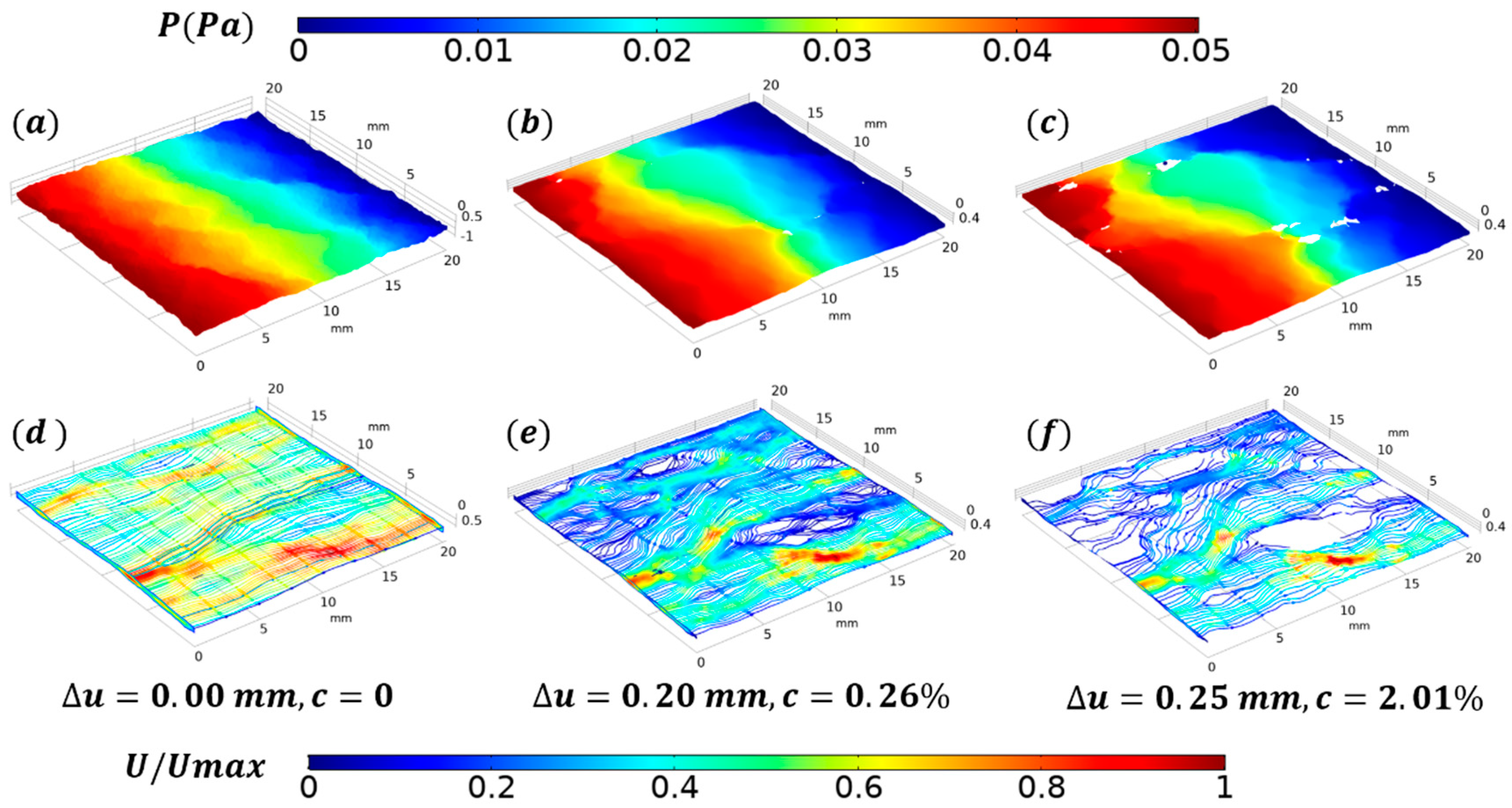
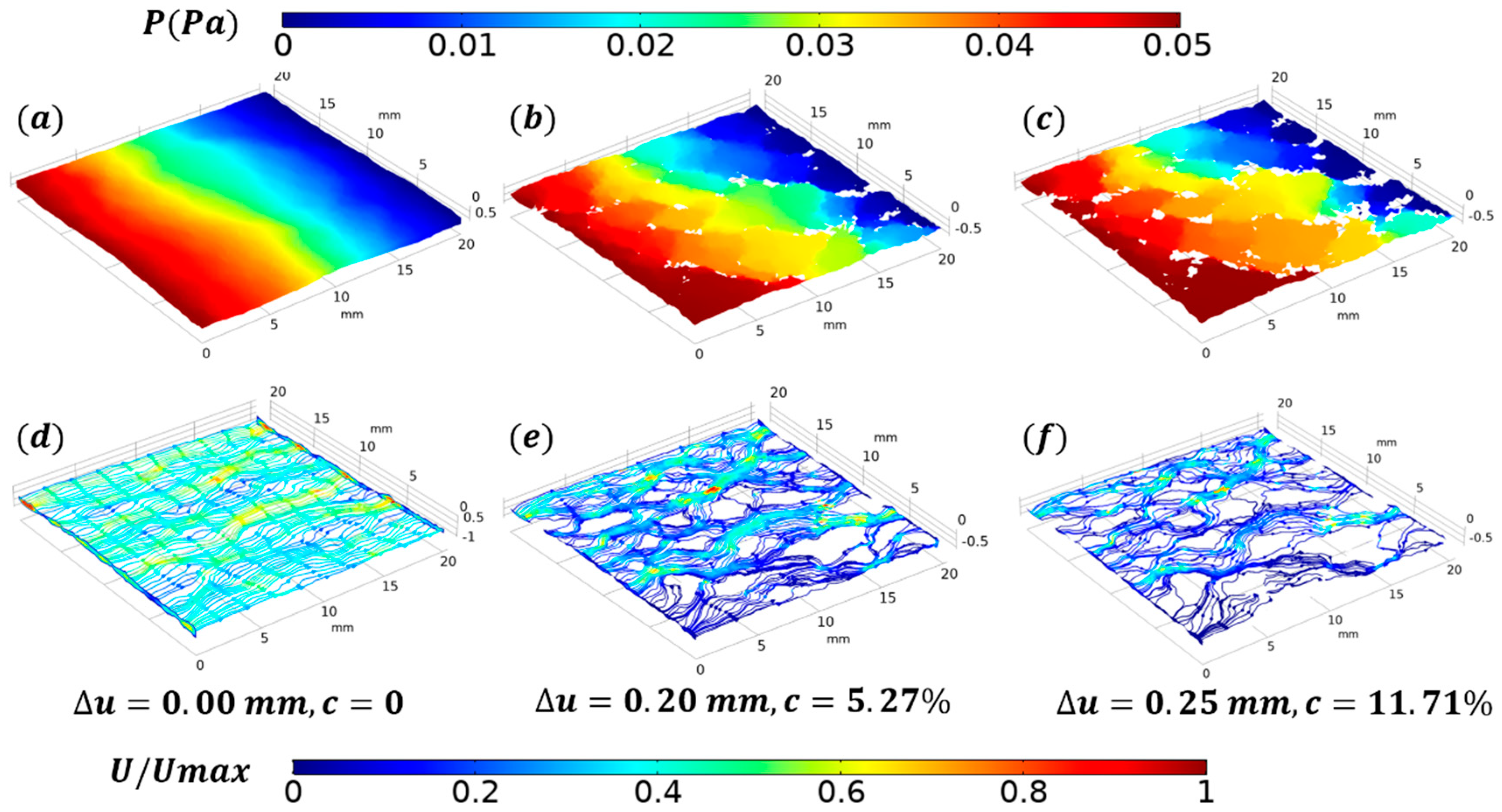
The numerical results for the fractures with H = 0.65 and H = 0.50 at three normal deformations of Δu = 0.00, 0.20, and 0.25 mm are used for illustration and comparison without loss of generality. Figure 6 and Figure 7 show the 3D distributions of the pressure, normalized velocity (U/Umax) and flow streamlines, respectively, during different normal deformations in fractures with H = 0.65 and 0.50. As can be seen in Figure 6a–c and Figure 7a–c, for the case of Δu = 0.00 mm, the iso-surface of the pressure is almost straight along the direction perpendicular to the flow (y-direction) and the pressure varies along the flow direction (x-direction) almost linearly in fractures with H = 0.65 and 0.50. However, as Δu increases, obvious heterogeneous or uneven distributions of the pressure start to appear in the fractures. This phenomenon is more obvious for smaller values of H with a dramatic increase in the contact area (Figure 7). These results are caused by the contact area and the local changes in the aperture, indicating that the contact area and surface roughness have a significant effect on the overall pressure distribution within the fractures.
As can be seen in Figure 6d–f and Figure 7d–f, the flow patterns throughout the fracture models change significantly with increasing Δu and decreasing H. For the case of Δu = 0.00 mm and H = 0.65 (see Figure 6d), the streamlines of the fluid flow are almost linearly distributed in the fracture domain. However, the normalized flow velocity (U/Umax) in Figure 6d was heterogeneously distributed within the fracture domain due to the variable distribution of the fracture aperture. As Δu increases, such as for the case of Δu = 0.25 mm and H = 0.65, the contact spots block off the flow and, thus, the streamlines go around the contact spots, resulting in preferential flow paths and a complex velocity distribution. As H decreases, such as for the case of Δu = 0.25 mm and H = 0.50, the streamlines are cut off by the widely spread contact areas, causing a significant decrease in the flow area. As a result, the actual flow paths and/or streamlines become more tortuous at larger Δu and smaller H. This phenomenon is the well-known channeling effect. At present, only numerical simulations can realistically illustrate the process of the complex evolution of flow localization (channeling) under different normal deformation conditions, since direct measurements and visualizations are not possible.
Figure 6d–f and Figure 7d–f also show that the flow is channeled into the main high-speed streams with many stagnant zones with very low velocities around the contact areas. It can also be found that the velocity field within a fracture with a smaller H and larger Δu is more complex, with the high velocity regions being more discretely distributed.
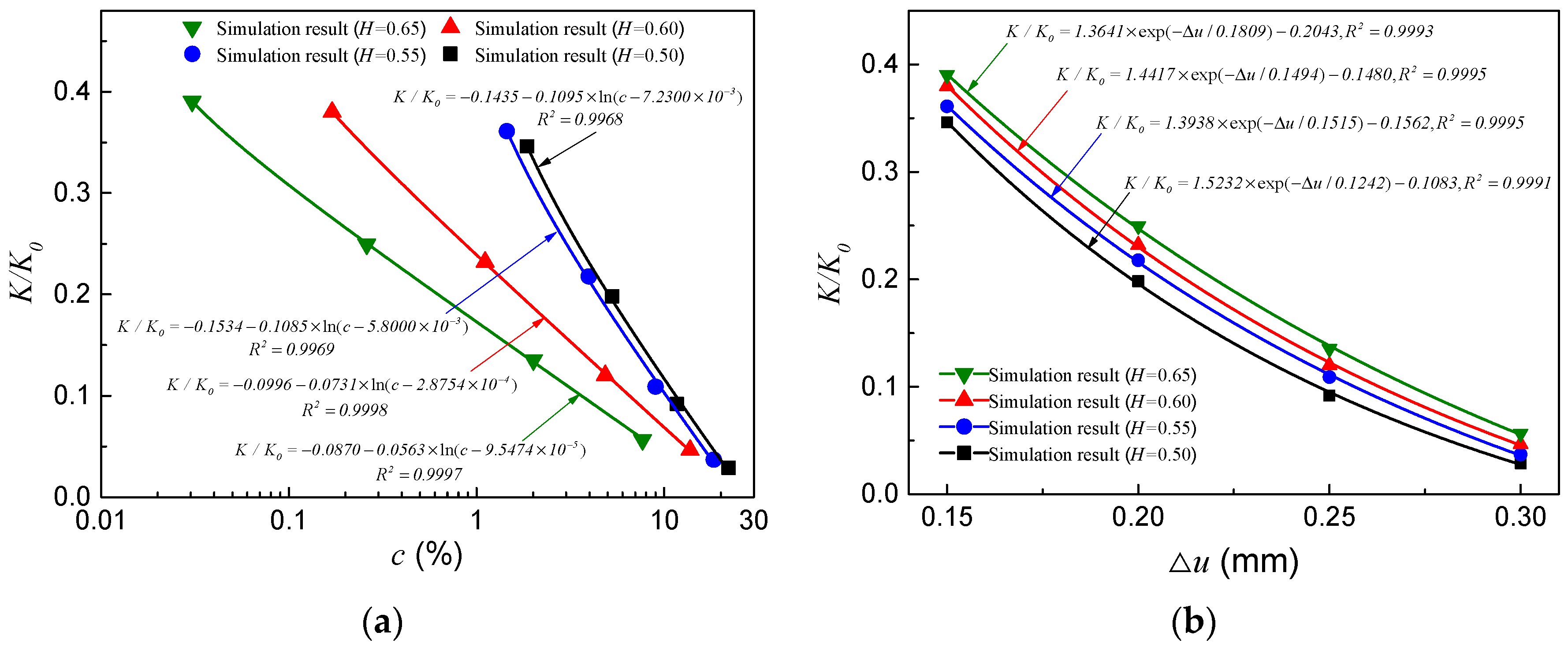
In order to analyze the influence of the normal deformation on the permeability of fractures with different H values, the relative permeability (K/K0), which relates the permeability at Δu (K) to the permeability at Δu = 0.00 mm (K0) in the flow direction, is calculated. Notably, the permeability in this study is macroscopic permeability of the fracture, which is obtained by Darcy’s law. The evolution of K/K0 for different H with respect to Δu and the contact area ratio c is displayed in Figure 8. For each fracture roughness, K/K0 decreases as Δu increases from 0.00 to 0.30 mm. In particular, when Δu = 0.30 mm, K/K0 reaches a minimum value and ranges from 0.029 to 0.057 with different H, indicating that the permeability for different roughness can be 17.5 or 34.5 times smaller than that at Δu = 0.00 mm. Comparisons of four fractures with the same Δu show that K/K0 increases as H increases, suggesting that under normal deformation conditions, permeability changes more in rougher fractures. The same evolution of K/K0 with respect to c is shown in Figure 8a. It should be noted that when c increases, the decrease in K/K0 for a smaller H is more significant than for larger H values. This is because the aperture distribution within the rougher fracture is more heterogeneous than that within the smoother fracture (as described in Section 2.2) which results in more tortuous flow paths, and thus a notable decrease in the permeability of the entire fracture.
4.2. Importance of Diffusion within the Fracture
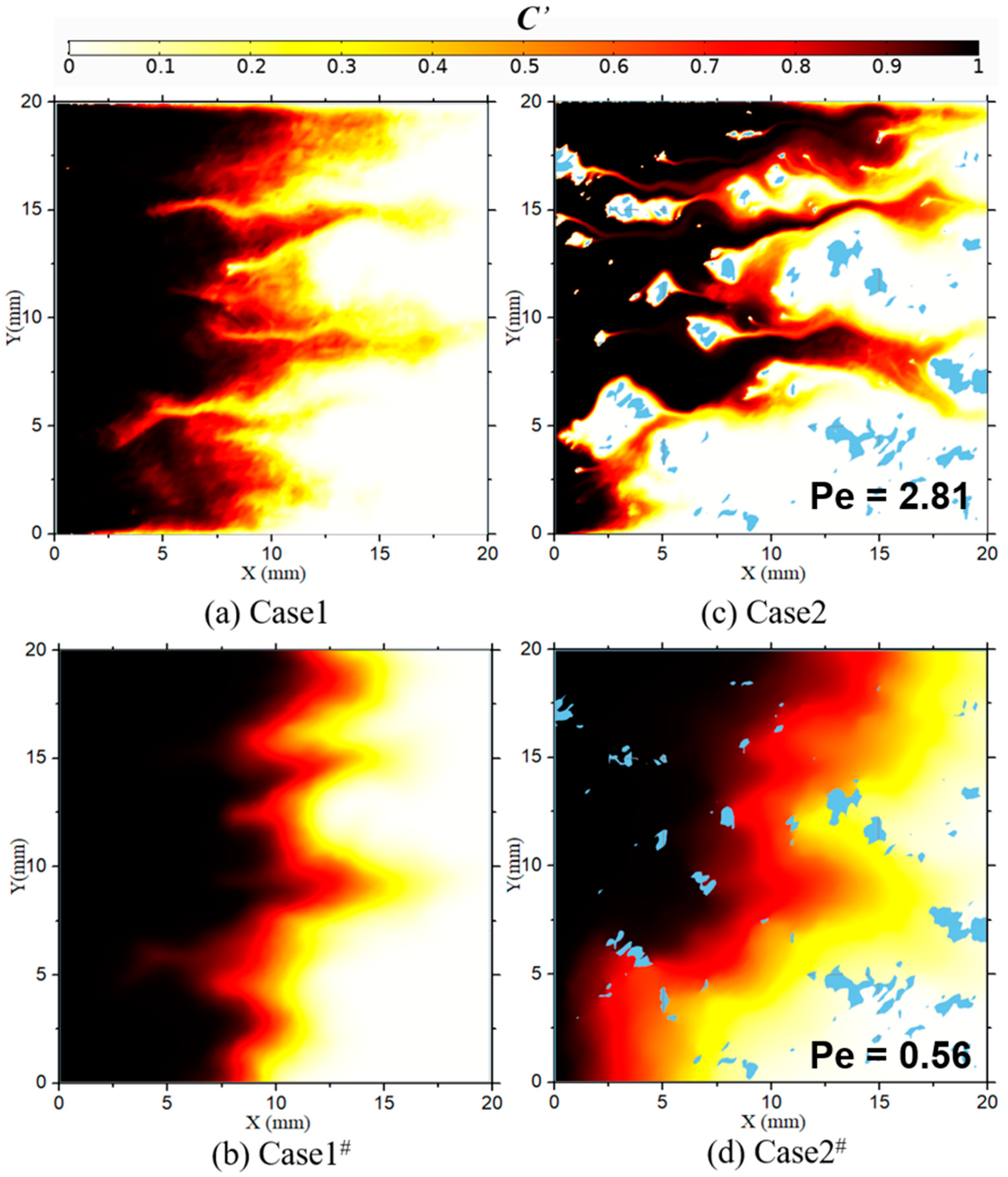
In this section, the numerical simulations that do not consider the diffusion process were carried out to illustrate the importance of the diffusion process in solute transport within a fracture. The simulation results of the concentration distribution at dimensionless time PV = 0.6 for H = 0.50 at Δu = 0.00 and 0.20 mm are presented in Figure 9a,c, respectively. For comparison, the corresponding simulation results considering the diffusion process are also plotted in Figure 9b,d.
The contour map of Case1 and Case2 shows that the concentration distributions are spotty and highly fragmented spread along the fractures. Additionally, the transport strongly follows preferential flow channels and exhibits notable fingering type transport paths. This transport behavior illustrates the fact that the flow heterogeneity caused by the complex geometric structure of the fracture roughness and contact areas (as described in Section 4.1) has a significant impact on the transport processes within the fracture.
As shown in Figure 9a,c, as Δu increases from 0.00 to 0.20 mm, the transport channels in Case 2 become more tortuous than those in Case1 due to the increased contact area ratio. As can be clearly seen in Figure 9c, the zones around the contact area are immobile domains where the dead zones with zero concentrations are formed. The reason for this is that the velocity around the contact area is almost 0; this cuts off the pathway for concentration transport into these zones when the absence of the diffusion obstructs the exchange of the concentration between the immobile zone (zero flow velocity) and the mobile zone (non-zero flow velocity).
In addition, the iso-surfaces of the concentration distributions in Case1 # and Case2 # are not as rough as those in Case1 and Case2, and the concentration fronts in Case1 and Case2 migrate faster than those in Case1 # and Case2 #, while the tails move slower than in Case1 # and Case2 #. This is due to the transverse redistribution of the concentration caused by the diffusion process, which slows down the speed of the solute fronts and enhances the mixing process in the tails. According to the analysis of Fried and Combarnous [68], both advection and diffusion contribute significantly to transport process when Pe between 0.4 and 5. Therefore, this comparison preliminarily validates the importance of the diffusion process in the evolution of the concentration field within the fractures, as the Pe numbers for Case1 # and Case2 # are 2.81 and 0.56, respectively, which indicates that the diffusion process is as important as the advection process. This finding is important in case of emergency pollution accidents in fractured rocks when the diffusion process is dominated or the value of Pe is between 0.4 and 5, according to previous study [68].
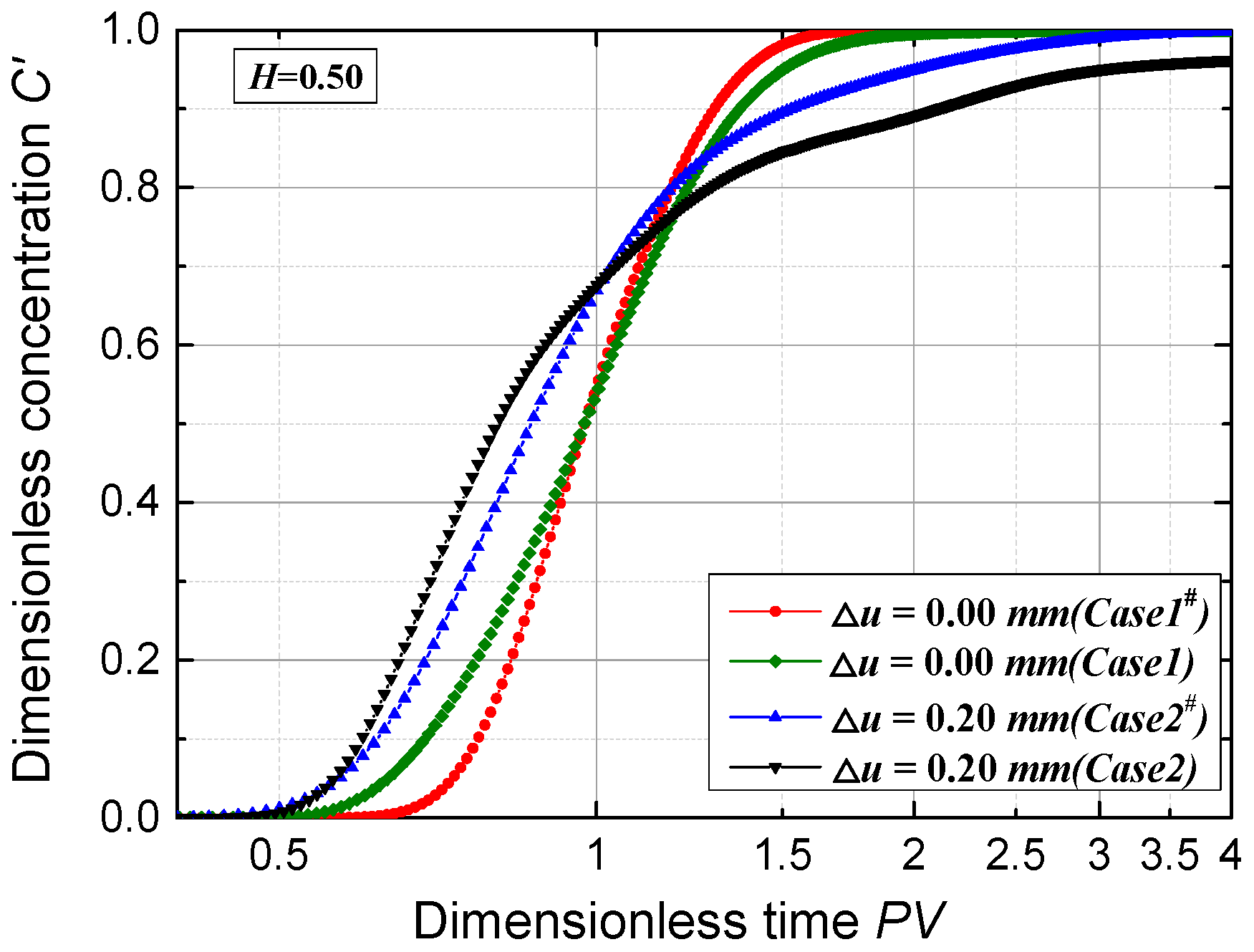
The flux-weighted BTCs calculated from the numerical simulations for Case1, Case1 #, Case2, and Case2 # are illustrated in Figure 10 to show the breakthrough features of the solute transport within the fractures with or without considering the diffusion process. As was explained in Section 3.2, the BTCs were calculated using continuous injection conditions. The transport for these cases is non-Fickian and exhibits early arrival and long tail characteristics. The early arrival and long tail in Case1 # and Case2 # are shortened and weakened, respectively, compared to those of Case1 or Case2, suggesting that the diffusion process notably affects the transport characteristics. Therefore, it is concluded that the final transport characteristics are caused by the combined effects of the advection and diffusion processes, which can be described by Pe.
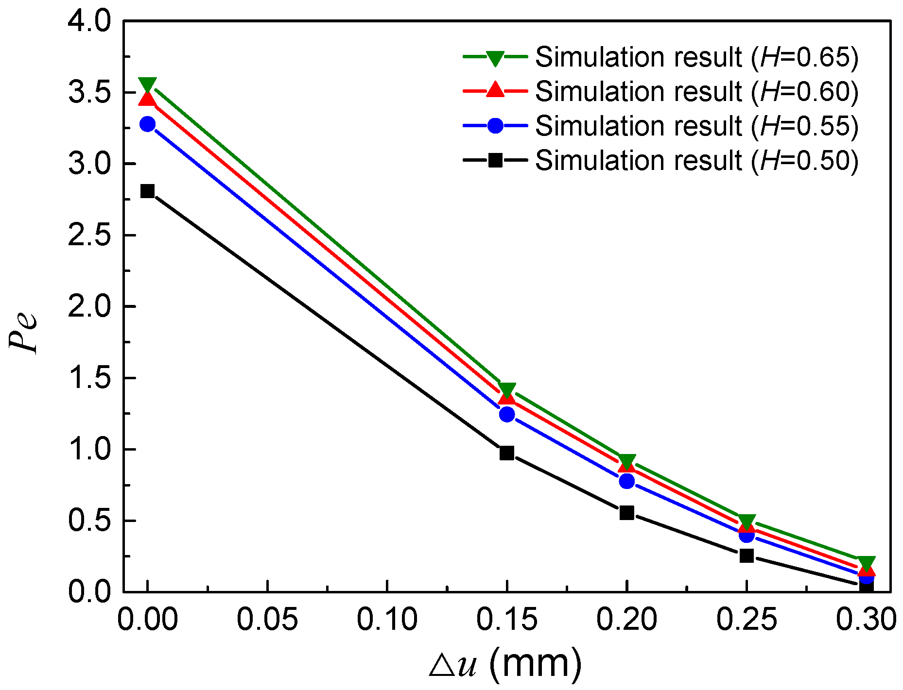
Figure 11 shows the values of Pe for the 20 simulation cases in this study. For a given fracture roughness, the Pe number decreases as Δu increases. It is clear that as Δu increases, the permeability of the fracture decreases and, thus, the flow rate (Q) in the fracture is decreased under the same pressure drop condition, resulting in a decrease in Pe. For all of the cases, the value of Pe ranges from 0.04 to 3.57. This indicates that both the diffusion term and the advection term are important for this study and, thus, they are taken into consideration in the following analysis.
4.3. Evolution of the Concentration Field
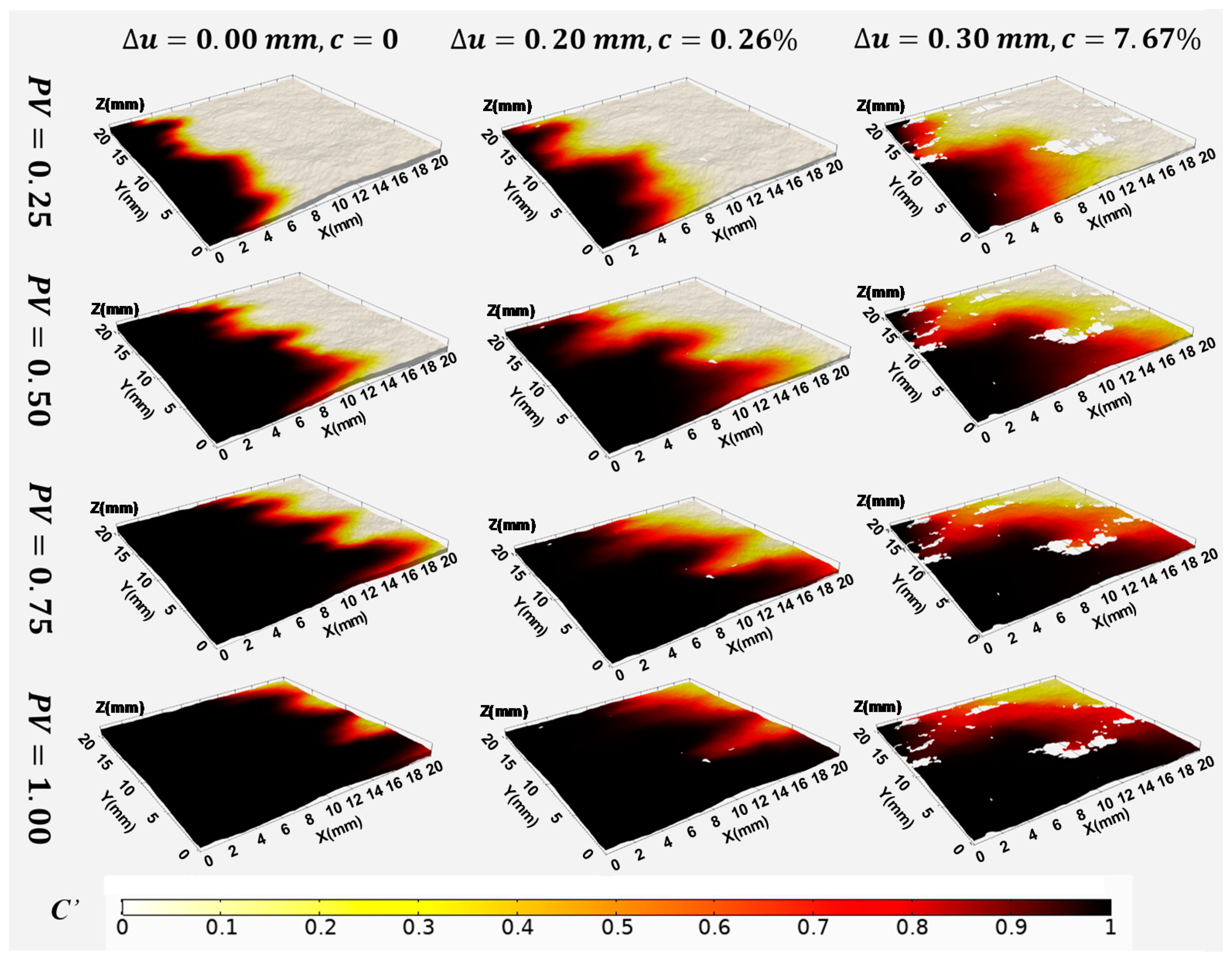
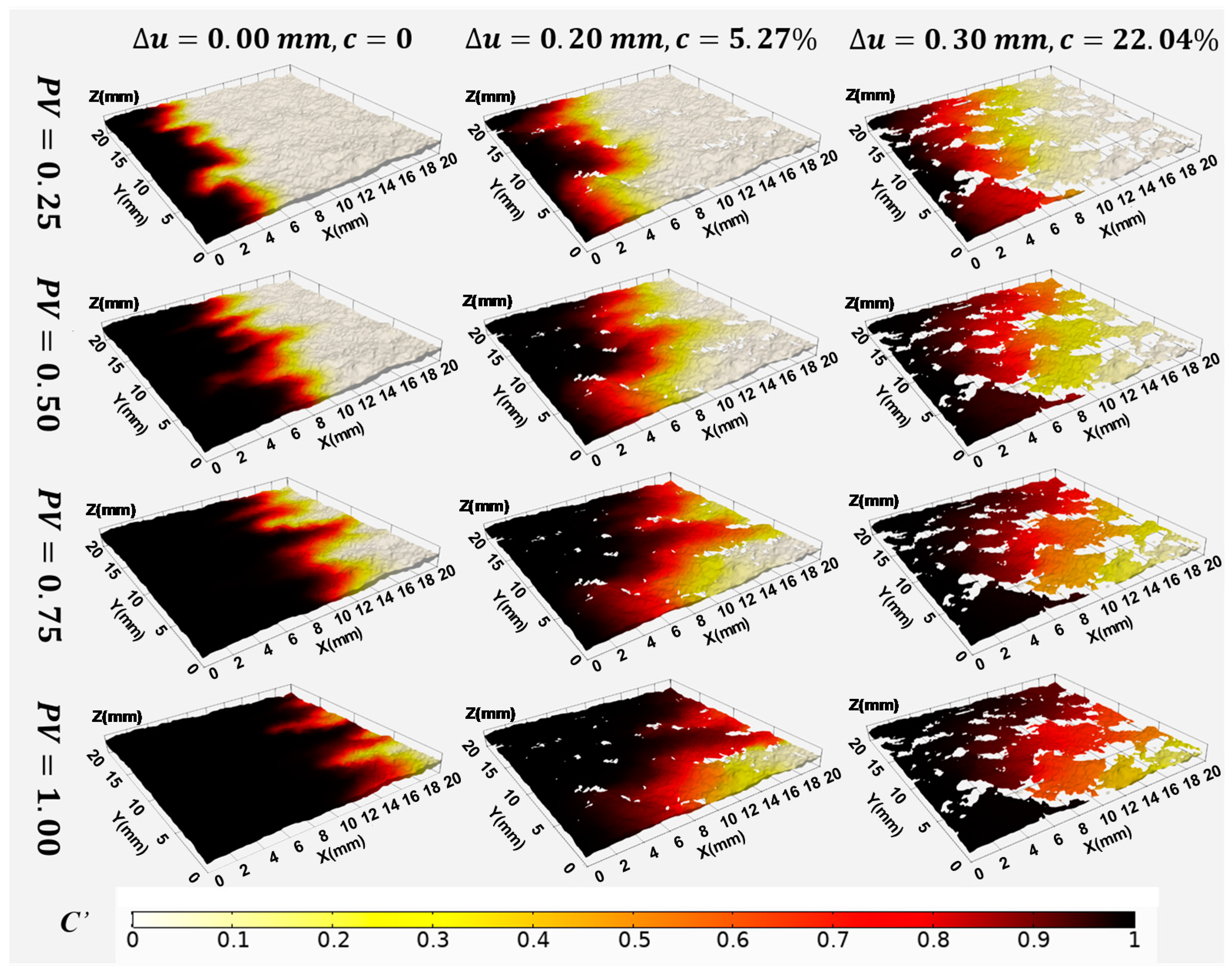
In order to investigate the influence of normal deformation and contact area on the spatial evolution of the solute, the same injected pore volumes (0.25, 0.50, 0.75, and 1.0 PV) in Figure 12 and Figure 13 were chosen for H = 0.65 and 0.50 with Δu = 0.00, 0.20, and 0.30 mm, respectively. As can be seen in Figure 12 and Figure 13, the evolution of the concentration field is sensitive to the contact area, especially for the cases with H = 0.50 (Figure 13). For the case of Δu = 0.00 mm (Figure 12a and Figure 13a), the spatial evolution of the solute is mainly affected by the surface roughness and aperture distribution of the fracture (c = 0). It clearly shows that there were several preferential channels of solute transport along the longitude direction of the fracture. This phenomenon may be explained by the fact that the flow velocity within the fracture was heterogeneously distributed due to the variable distribution of the fracture aperture, as stated in Section 3.1. In addition, the transport process is dominated by advection within the fracture, i.e., the Pe numbers in the cases are larger than 1.0 (Pe = 3.57 for H = 0.65 and Pe = 2.81 for H = 0.50). When Δu increases from 0.00 to 0.20 mm (Figure 12b and Figure 13b), the contact area increases in the relatively small aperture regions (c = 5.27% for H = 0.50, and c = 0.26% for H = 0.65). The solute around the zones with contact areas exhibited slower transport than the zones without contact areas. When Δu increases from 0.20 to 0.30 mm (Figure 12c and Figure 13c), the solute around the contact areas is further delayed; however, the fingering type transport disappears gradually compared to the cases with Δu = 0.00 mm. This is because of the low Pe numbers in the cases with Δu = 0.30 mm (i.e., Pe = 0.21 for H = 0.65 and Pe = 0.04 for H = 0.50), which indicates that the transport is dominated by diffusion. As a result, the preferential transport caused by the channeling effects is masked by the diffusion process. Nevertheless, due to the dominance of the diffusion process, the movement of the solute in the cases with Δu = 0.30 mm is still faster than in the cases with smaller Δu.
For all of the cases, based on the analysis in Section 4.2, we conclude that the solute first passes without penetrating the zones near contacts, then, it invades them due to the diffusion. These contact areas result in the formation of an immobile region and can provide strong resistance against spreading and mixing. Consequently, the transport of the solute is significantly delayed by the contact areas, as shown in the cases of Δu = 0.30 mm in Figure 12c and Figure 13c.
4.4. BTCs, First Arrival Times and the Residence Time Distributions (RTDs)
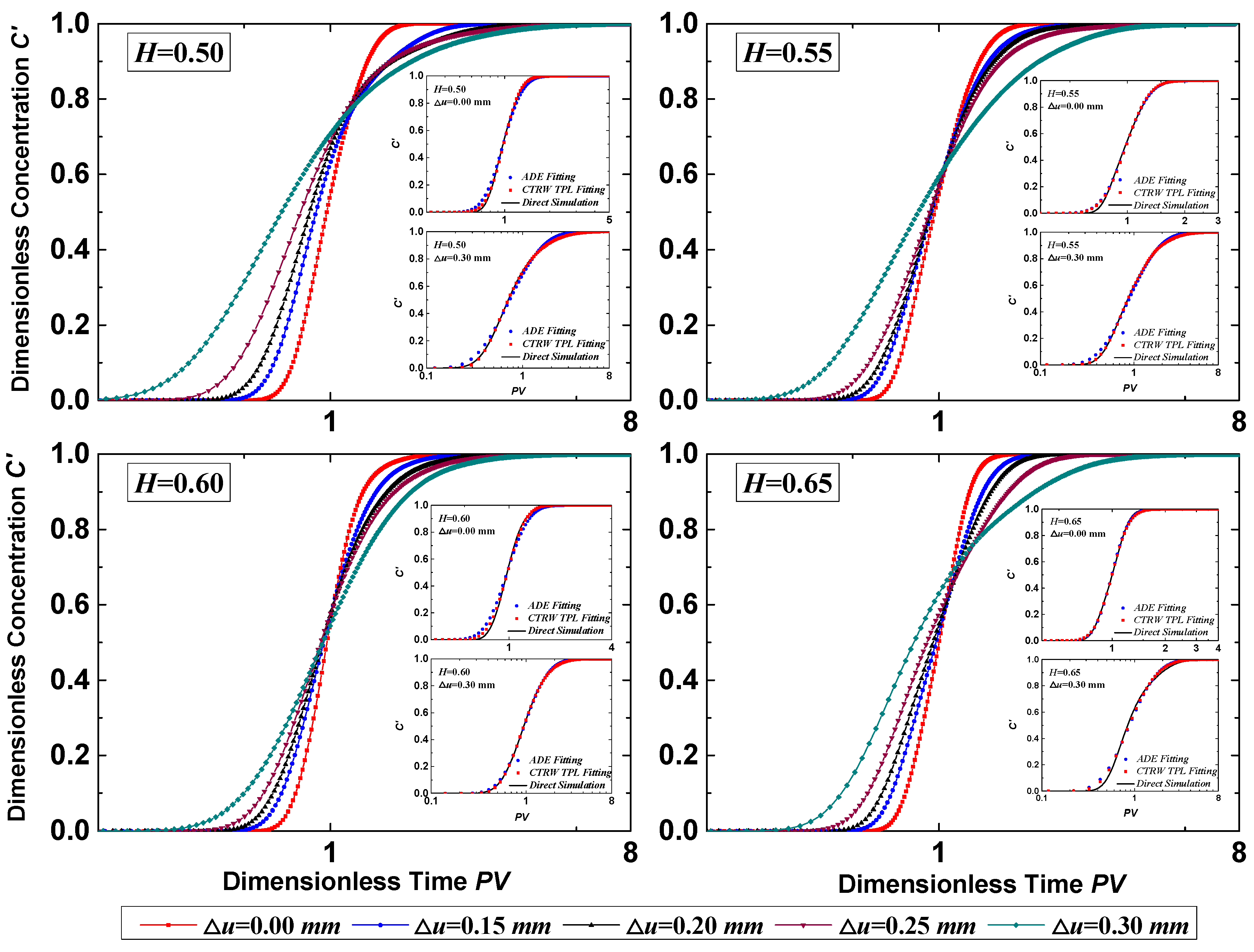
In order to analyze the influence of the contact area ratio and normal deformation on solute transport, the corresponding flux-weighted BTCs were calculated for different values of H and Δu, as shown in Figure 14. The typical early arrival and long tail characteristics were observed in all of the BTCs, indicating non-Fickian transport. As was discussed in Section 4.1 and Section 4.2, the preferential transport caused by the complex aperture distribution and contact area was likely responsible for the ubiquitous non-Fickian transport. In fact, for the cases with Δu = 0.00 mm, the non-Fickian characteristics were not obvious. However, the early arrival tends to be enhanced as Δu increases, which is directly caused by the enhanced preferential transport and diffusion process within the fracture, as stated in Section 4.2 and Section 4.3.
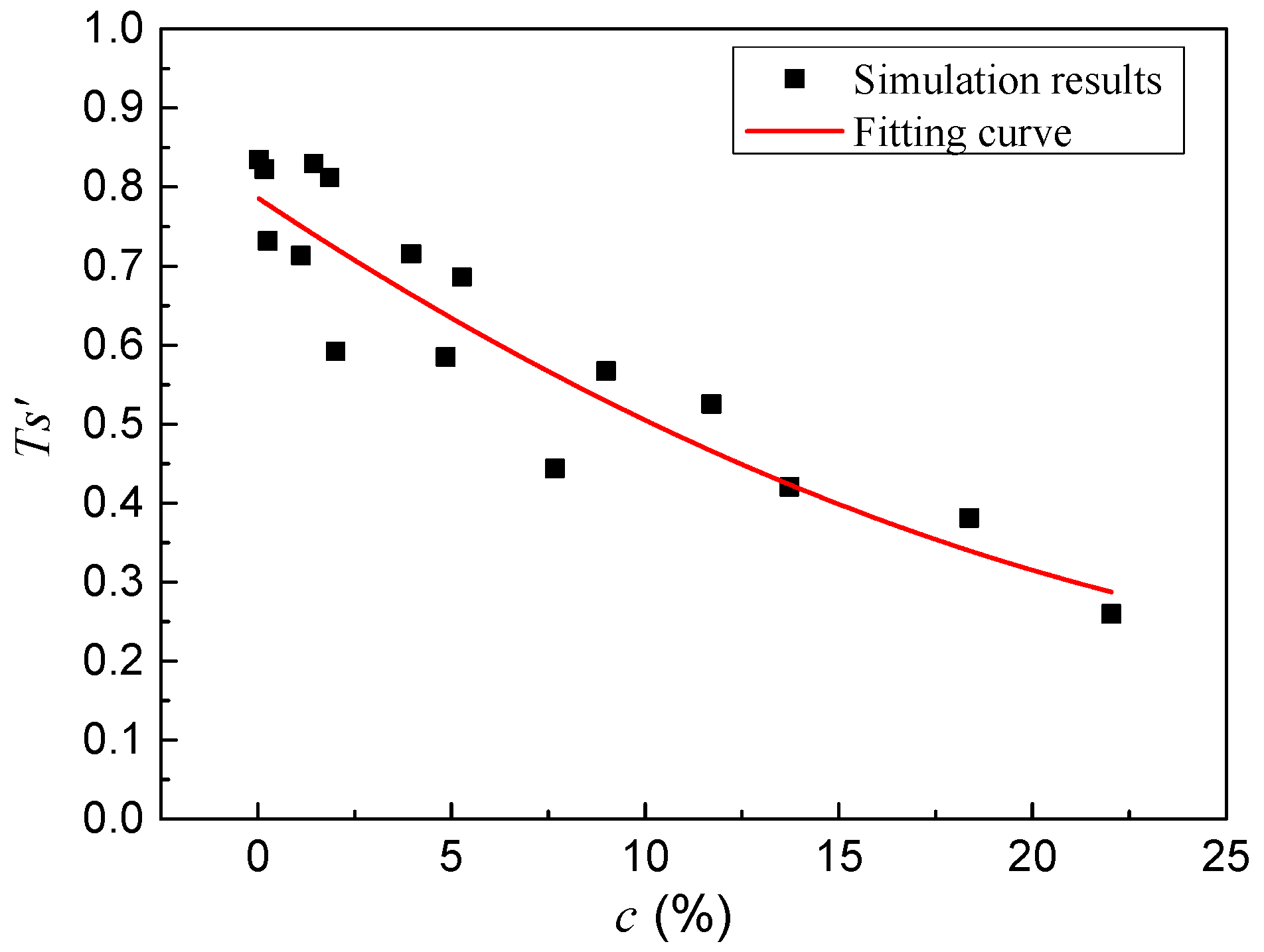
To quantify the relationship between the observed early arrival characteristic and the contact area ratio c in Figure 14, the normalized first breakthrough time Ts′ of the solute transport was calculated using
where Ts is the first breakthrough time (when C′ equals 1 × 10⁻⁵) for Δu = 0.15, 0.20, 0.25, and 0.30 mm, and is the first breakthrough time for Δu = 0.00 mm.
Figure 15 shows the relationship between Ts′ and c for all numerical simulation cases. The results show that as c increases, Ts′ decreases rapidly, and it is less than 0.83 when c ≥ 0.03%. In particular, when c = 22.04%, Ts′ reaches a minimum value of 0.26, indicating that the contact area ratio significantly affects the breakthrough time of the solute transport within the fractures.
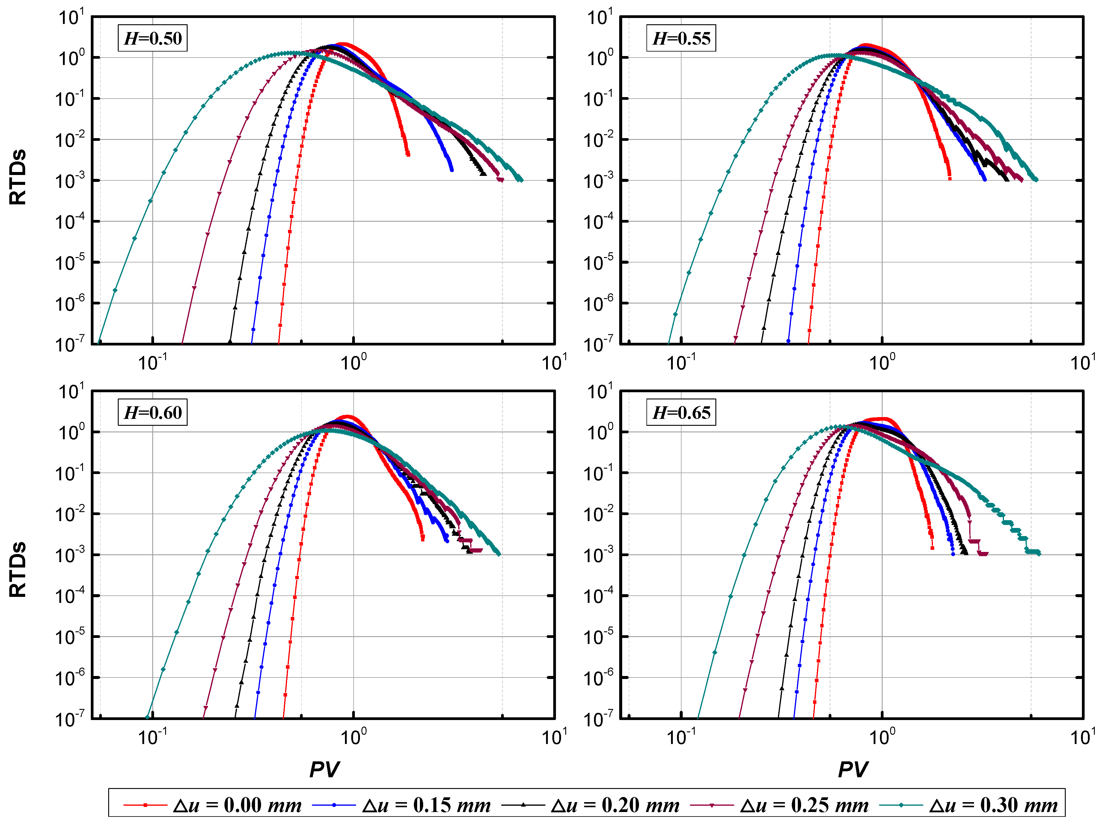
According to the behaviors of the velocity fields and concentration fields within the fracture domain (Section 4.1 and Section 4.3), the presence and development of the contact areas within the rough-walled fractures divide the fracture into immobile and mobile regions, which represent the zero-velocity or low-velocity zone and the relatively high-velocity zone, respectively. This mobile-immobile region causes solute exchange between the two regions across the fracture aperture because of the solute diffusion mechanism. Thus, this phenomenon is most likely responsible for the long tails of the BTCs. In order to characterize the long tail characteristics of the BTCs, the residence time distributions (RTDs) were calculated for the solute transport within the fractures under different normal deformations. In this study, the RTDs were derived from the time derivative of the BTCs, . Figure 16 shows the RTDs for solute transport through the fractures for different values of H and Δu. The tail after the peak is apparent in the RTDs and follows a power-law drop (especially for large Δu). The degree of the power-law drop increases as Δu increases. This is attributed to the increase in the number of contact spots cutting off the transport channels, thus increasing the arrival time of the solute at the fracture outlet.
4.5. Uniformity of the Concentration Distribution within the Fracture
The numerical simulations revealed the important non-uniform concentration distribution within the fracture caused by the surface roughness and the contact areas, especially when the contact area ratio c increases (see Figure 12 and Figure 13). As can be found in Figure 6, Figure 7, Figure 12 and Figure 13, the solute concentration in the main flow channel is higher than that in other channels, especially the low velocity zones. However, this non-uniform concentration distribution tends to be uniform for continuously injected solute. The evolution from non-uniform to uniform concentration distribution determines the magnitude of the tails of the BTCs, i.e., the longer the evolution process, the heavier the tail. Here, the metric of concentration distribution index (CDI) proposed in our previous study [15] is applied to quantify the properties of the non-uniform concentration distribution. The CDI is defined as the ratio between the total solute concentration within the full-scale fracture domain at dimensionless time or PV and the solute concentration of the uniform distribution state, which is mathematically equal to the volume of the entire fracture. The CDI is given by
where is the fracture domain or integral domain, and (kg/m3) is the solute concentration within the fracture at dimensionless time or PV. It should be noted that the larger the value of , the more uniform the concentration distribution within the fracture domain.
Figure 17 illustrates the temporal evolution of CDI for H = 0.50, 0.55, 0.60, and 0.65 and Δu = 0.15, 0.20, 0.25, and 0.30 mm. For all of the cases, CDI was less than 1.0 after one PV, suggesting the presence of the non-uniform concentration distribution within the fracture. The CDI value at PV = 1.0 was analyzed to quantify the differences between various rough fractures with different normal deformation values (Figure 18). As can be seen in Figure 18, the CDI at PV = 1.0 decreased as Δu increases, suggesting that increasing the contact area enhances the non-uniform concentration distribution within the fracture domain. This is likely the reason that the transport channel becomes more complex with increasing contact area, leading to a longer time for the solute to spread and mix around the contact spots, thereby delaying the time required to reach a uniform distribution (CDI = 1.0). Therefore, for large Δu, heavier tails were observed in the BTCs and RTDs.
Figure 18a,b show the CDI as a function of the roughness parameter H for different normal deformation levels and as a function of Δu for different H, respectively. As can be seen in Figure 18a, the fitted trend lines vary linearly with increasing H for increasing CDI, and CDI is larger than 0.90 when Δu = 0.00 mm, while it is smaller than 0.8 when Δu = 0.30 mm, indicating that surface roughness has an important effect on the spreading and mixing process in solute transport. In contrast, when Δu increases, the CDI decreases exponentially (Figure 18b), indicating that the increased c, caused by the normal deformation, results in a longer time for the solute/contaminant to fill the entire fracture. Therefore, the contact area within the fracture plays an important role in delaying the solute exchange between the region around the contact areas and the main flow channel, which directly results in the tails of BTCs.
4.6. Inverse Model for Non-Fickian BTCs
To further investigate the impact of contact area on the non-Fickian transport behavior, the ADE and CTRW models were used to fit all of the BTCs in this study. The inserted subfigures in Figure 14 show the best-fit results of the BTCs using the ADE and CTRW models. The root mean square error (RMSE) was introduced to quantify the goodness-of-fit, which is given as follows:
where and represent the solute’s concentration at the ith point to be compared with the fitting results and the numerical results, respectively; N is the number of data points in the BTC.
Figure 19 shows the boxplots of the RMSE of the BTCs between the numerical simulations and the fitted results for all cases. The boxplots in Figure 19 reveal that the mean, maximum, and minimum values of the CRTW fitting are smaller than the ADE fitting, and the RMSE of the CTRW fittings is smaller than 1%, indicating that the best-fit results of the BTCs from the CTRW model are better than those from the ADE model. This is because the TPL model embedded in the CTRW is capable of capturing the early arrival and long tail phenomena, while the ADE falls short. Physically, the difference between these two models is that the TPL–CTRW model uses a transition probability function that allows for local heterogeneity, so it more accurately models the actual solute transport dynamics, while the ADE inherently treats heterogeneous fractures as homogeneous media with a flow velocity and dispersion coefficient that are constant in space and time.
β is the estimated parameter of the CTRW model for the numerical simulation cases, and it is often applied as a metric for quantifying the degree of non-Fickian transport. Therefore, analyzing β provides insight into the mechanism of the impact of contact area on non-Fickian transport. As can be seen in Figure 20, β mostly ranges from 0.8 to 2, indicating a moderate non-Fickian transport regime for these cases, as described in Section 3.3.2. As can be seen in Figure 20a, the estimated β is smaller within the fracture for lower H values, indicating that increased surface roughness enhances the heterogeneity of the solute transport or non-Fickian transport. In addition, Figure 20b,c show that β decreases exponential as Δu and/or c increase, further suggesting that the normal deformation-induced contact area plays a critical role in non-Fickian transport within the rough-walled fracture. The connections we established between β and H, Δu and c allow for the upscaling of the effects of local spreading and mixing processes around the contact areas within the CTRW framework, at least for 3D single rough-walled fractures.
5. Conclusions and Suggestions
In this study, a series of 3D self-affine fractal models were established to study the combined effects of surface roughness and the contact area on non-Fickian transport. Fractures with different surface roughnesses (H) were considered. The fracture surfaces were generated using the modified successive random addition (SRA) method. Normal deformation (Δu) was applied on the upper surface by fixing the lower surface. The evolutions of the aperture distribution and contact area ratio (c) within the deformed rough-walled fractures were analyzed. In addition, the flow and transport problem through the deformed rough-walled fractures was solved. The influence of Δu and c on the flow paths, permeability, and non-Fickian transport was estimated. The non-Fickian transport properties resulting from H, Δu, and c were systematically investigated. The following conclusions were drawn from the results of this study:
- (1)
- As Δu increases, the contact area between the two fracture surfaces increases and more void spaces are reduced. The streamlines within the rough-walled fractures show that the contact areas block off the flow and, thus, the streamlines go around the contact areas, resulting in preferential flow paths and a complex velocity distribution. The spatial evolution of the solute within the fractures for different c values shows that the transport exhibits a strong channeling effect and notable fingering type transport paths, indicating that the contact conditions have a crucial effect on the flow paths and solute transport.
- (2)
- The non-Fickian early arrival and long tail characteristics in all of the BTCs for fractures with different Δu and H values were captured. The normalized first breakthrough time (Ts’) at the outlet for different c values was used to quantify the characteristic of the early arrival of the BTCs. As c varies from 0% to 22.04%, Ts’ decreases from 0.83 to 0.26, indicating that the breakthrough time of solute transport is shortened as the contact area ratio increases.
- (3)
- The uniformity of the concentration distribution within the fracture was quantified using the concept of the concentration–dilution index. The temporal evolution of the dilution index reveals that the immobile zone around the developing contact areas provides strong resistance to solute transport and delays the solute exchange with the main flow channel. We conclude that the dilution index at a given pore volume (PV) can effectively describe the relationship between the magnitude of the tails of the BTCs and the delayed rate of solute exchange. Although the solute exchange processes between the main flow channel and the contact area cannot be directly quantified, our results qualitatively highlight the fact that the tails are caused by the increasing contact area and surface roughness.
- (4)
- The CTRW–TPL model is quite capable of capturing the effect of contact area ratio on non-Fickian transport in 3D rough-walled fractures. The estimated β values of the CTRW model decrease from 1.92 to 0.81 as c increases from 0% to 22.04% and H decreases from 0.65 to 0.50, indicating that the developed contact area and rougher fracture surface increase the magnitude of the non-Fickian transport. The connections we established between β and Δu and c allow for the upscaling of the effects of the local spreading and mixing processes around the contact areas within the CTRW framework, at least for 3D single rough-walled fractures.
Author Contributions
Conceptualization, W.X. and Y.H.; methodology, Y.H. and Z.Y.; software, Y.H.; validation, Y.H.; formal analysis, W.X., Y.H. and Z.Y.; investigation, Y.H.; resources, W.X. and Y.H.; data curation, Y.H.; writing—original draft preparation, Y.H.; writing—review and editing, W.X. and L.Z.; visualization, Y.H.; supervision, W.X. and L.Z.; project administration, L.Z. and Y.C.; funding acquisition, L.Z. and Y.C. All authors have read and agreed to the published version of the manuscript.
Funding
The study is financially supported by the National Funds for Distinguished Young Scholars of China (Grant Nos. 51625805), the National Key Research and Development Project (Grant Nos. 2018YFC1802300) and the National Natural Science Foundation of China (No. 51988101).
Conflicts of Interest
The authors declare no conflict of interest.
References
- Zhou, R.; Zhan, H. Reactive solute transport in an asymmetrical fracture–rock matrix system. Adv. Water Resour. 2018, 112, 224–234. [Google Scholar] [CrossRef]
- Wang, L.; Bayani Cardenas, M. Transition from non-Fickian to Fickian longitudinal transport through 3-D rough fractures: Scale-(in)sensitivity and roughness dependence. J. Contam. Hydrol. 2017, 198, 1–10. [Google Scholar] [CrossRef] [Green Version]
- Cvetkovic, V.; Frampton, A. Solute transport and retention in three-dimensional fracture networks. Water Resour. Res. 2012, 48, 419–420. [Google Scholar] [CrossRef]
- Zhao, Z.; Jing, L.; Neretnieks, I.; Moreno, L. Numerical modeling of stress effects on solute transport in fractured rocks. Comput. Geotech. 2011, 38, 113–126. [Google Scholar] [CrossRef]
- Bodin, J.; Delay, F.; de Marsily, G. Solute transport in a single fracture with negligible matrix permeability: 1. fundamental mechanisms. Hydrogeol. J. 2003, 11, 418–433. [Google Scholar] [CrossRef]
- Berkowitz, B. Characterizing flow and transport in fractured geological media: A review. Adv. Water Resour. 2002, 25, 861–884. [Google Scholar] [CrossRef]
- Moreno, L.; Neretnieks, I. Fluid flow and solute transport in a network of channels. J. Contam. Hydrol. 1993, 14, 163–192. [Google Scholar] [CrossRef]
- Zhou, J.; Wang, L.; Chen, Y.; Cardenas, M.B. Mass Transfer Between Recirculation and Main Flow Zones: Is Physically Based Parameterization Possible? Water Resour. Res. 2019, 55, 345–362. [Google Scholar] [CrossRef] [Green Version]
- Dou, Z.; Sleep, B.; Zhan, H.; Zhou, Z.; Wang, J. Multiscale roughness influence on conservative solute transport in self-affine fractures. Int. J. Heat Mass Transf. 2019, 133, 606–618. [Google Scholar] [CrossRef]
- Zou, L.; Jing, L.; Cvetkovic, V. Modeling of Solute Transport in a 3D Rough-Walled Fracture–Matrix System. Transp. Porous Media 2017, 116, 1005–1029. [Google Scholar] [CrossRef] [Green Version]
- Kang, P.K.; Dentz, M.; Le Borgne, T.; Juanes, R. Anomalous transport on regular fracture networks: Impact of conductivity heterogeneity and mixing at fracture intersections. Phys. Rev. E 2015, 92, 22148. [Google Scholar] [CrossRef] [PubMed] [Green Version]
- Geiger, S.; Cortis, A.; Birkholzer, J.T. Upscaling solute transport in naturally fractured porous media with the continuous time random walk method. Water Resour. Res. 2010, 46, 264–278. [Google Scholar] [CrossRef] [Green Version]
- Berkowitz, B.; Scher, H. Anomalous Transport in Random Fracture Networks. Phys. Rev. Lett. 1997, 79, 4038–4041. [Google Scholar] [CrossRef]
- Chen, Z.; Zhan, H.; Zhao, G.; Huang, Y.; Tan, Y. Effect of Roughness on Conservative Solute Transport through Synthetic Rough Single Fractures. Water 2017, 9, 656. [Google Scholar] [CrossRef] [Green Version]
- Hu, Y.; Xu, W.; Zhan, L.; Li, J.; Chen, Y. Quantitative characterization of solute transport in fractures with different surface roughness based on ten Barton profiles. Environ. Sci. Pollut. Res. 2020, 27, 13534–13549. [Google Scholar] [CrossRef]
- Carrera, J.; Sánchez-Vila, X.; Benet, I.; Medina, A.; Galarza, G.; Guimerà, J. On matrix diffusion: Formulations, solution methods and qualitative effects. Hydrogeol. J. 1998, 6, 178–190. [Google Scholar] [CrossRef]
- Zhu, Y.; Zhan, H. Quantification of solute penetration in an asymmetric fracture-matrix system. J. Hydrol. 2018, 563, 586–598. [Google Scholar] [CrossRef]
- Zou, L.; Jing, L.; Cvetkovic, V. Modeling of flow and mixing in 3D rough-walled rock fracture intersections. Adv. Water Resour. 2017, 107, 1–9. [Google Scholar] [CrossRef]
- Zhu, Y.; Zhan, H.; Jin, M. Analytical solutions of solute transport in a fracture–matrix system with different reaction rates for fracture and matrix. J. Hydrol. 2016, 539, 447–456. [Google Scholar] [CrossRef]
- Becker, M.W.; Shapiro, A.M. Tracer transport in fractured crystalline rock: Evidence of nondiffusive breakthrough tailing. Water Resour. Res. 2000, 36, 1677–1686. [Google Scholar] [CrossRef] [Green Version]
- Silva, J.A.; Kang, P.K.; Yang, Z.; Cueto Felgueroso, L.; Juanes, R. Impact of Confining Stress on Capillary Pressure Behavior during Drainage through Rough Fractures. Geophys. Res. Lett. 2019, 46, 7424–7436. [Google Scholar] [CrossRef] [Green Version]
- Huo, D.; Benson, S.M. Experimental Investigation of Stress-Dependency of Relative Permeability in Rock Fractures. Transport. Porous Med. 2016, 113, 567–590. [Google Scholar] [CrossRef]
- Watanabe, N.; Sakurai, K.; Ishibashi, T.; Ohsaki, Y.; Tamagawa, T.; Yagi, M.; Tsuchiya, N. Newν-type relative permeability curves for two-phase flows through subsurface fractures. Water Resour. Res. 2015, 51, 2807–2824. [Google Scholar] [CrossRef]
- Bertels, S.P.; DiCarlo, D.A.; Blunt, M.J. Measurement of aperture distribution, capillary pressure, relative permeability, and in situ saturation in a rock fracture using computed tomography scanning. Water Resour. Res. 2001, 37, 649–662. [Google Scholar] [CrossRef] [Green Version]
- Zhou, J.; Hu, S.; Fang, S.; Chen, Y.; Zhou, C. Nonlinear flow behavior at low Reynolds numbers through rough-walled fractures subjected to normal compressive loading. Int. J. Rock Mech. Min. Sci. 2015, 80, 202–218. [Google Scholar] [CrossRef]
- Chen, Y.; Lian, H.; Liang, W.; Yang, J.; Nguyen, V.P.; Bordas, S.P.A. The influence of fracture geometry variation on non-Darcy flow in fractures under confining stresses. Int. J. Rock Mech. Min. Sci. 2019, 113, 59–71. [Google Scholar] [CrossRef]
- Vogler, D.; Settgast, R.R.; Annavarapu, C.; Madonna, C.; Bayer, P.; Amann, F. Experiments and Simulations of Fully Hydro-Mechanically Coupled Response of Rough Fractures Exposed to High-Pressure Fluid Injection. J. Geophys. Res. Solid Earth 2018, 123, 1186–1200. [Google Scholar] [CrossRef]
- Liu, R.; Huang, N.; Jiang, Y.; Jing, H.; Yu, L. A numerical study of shear-induced evolutions of geometric and hydraulic properties of self-affine rough-walled rock fractures. Int. J. Rock Mech. Min. Sci. 2020, 127, 104211. [Google Scholar] [CrossRef]
- Jeong, W.; Song, J. Numerical Investigations for Flow and Transport in a Rough Fracture with a Hydromechanical Effect. Energy Sources 2005, 27, 997–1011. [Google Scholar] [CrossRef]
- Koyama, T.; Li, B.; Jiang, Y.; Jing, L. Numerical simulations for the effects of normal loading on particle transport in rock fractures during shear. Int. J. Rock Mech. Min. Sci. 2008, 45, 1403–1419. [Google Scholar] [CrossRef] [Green Version]
- Kang, P.K.; Brown, S.; Juanes, R. Emergence of anomalous transport in stressed rough fractures. Earth Planet. Sci. Lett. 2016, 454, 46–54. [Google Scholar] [CrossRef] [Green Version]
- Benson, D.A.; Wheatcraft, S.W.; Meerschaert, M.M. Application of a fractional advection-dispersion equation. Water Resour. Res. 2000, 36, 1403–1412. [Google Scholar] [CrossRef] [Green Version]
- Cherubini, C.; Giasi, C.I.; Pastore, N. Evidence of non-Darcy flow and non-Fickian transport in fractured media at laboratory scale. Hydrol. Earth Syst. Sci. 2013, 17, 2599–2611. [Google Scholar] [CrossRef] [Green Version]
- Dou, Z.; Chen, Z.; Zhou, Z.; Wang, J.; Huang, Y. Influence of eddies on conservative solute transport through a 2D single self-affine fracture. Int. J. Heat Mass Transf. 2018, 121, 597–606. [Google Scholar] [CrossRef]
- Haggerty, R.; Gorelick, S.M. Multiple-Rate Mass Transfer for Modeling Diffusion and Surface Reactions in Media with Pore-Scale Heterogeneity. Water Resour. Res. 1995, 31, 2383–2400. [Google Scholar] [CrossRef]
- Wang, L.; Cardenas, M.B. Non-Fickian transport through two-dimensional rough fractures: Assessment and prediction. Water Resour. Res. 2014, 50, 871–884. [Google Scholar] [CrossRef]
- Berkowitz, B.; Cortis, A.; Dentz, M.; Scher, H. Modeling non-Fickian transport in geological formations as a continuous time random walk. Rev. Geophys. 2006, 44, G2003. [Google Scholar] [CrossRef] [Green Version]
- Brown, S.R.; Scholz, C.H. Broad bandwidth study of the topography of natural rock surfaces. J. Geophys. Res. Solid Earth 1985, 90, 12575–12582. [Google Scholar] [CrossRef]
- Mandelbrot, B.B.; Pignoni, R. The Fractal Geometry of Nature; W. H. Freeman and Company: London, UK, 1983. [Google Scholar]
- Odling, N.E. Natural fracture profiles, fractal dimension and joint roughness coefficients. Rock Mech. Rock Eng. 1994, 27, 135–153. [Google Scholar] [CrossRef]
- Belem, T.; Homand-Etienne, F.; Souley, M. Fractal analysis of shear joint roughness. Int. J. Rock Mech. Min. Sci. 1997, 34, 130–131. [Google Scholar] [CrossRef]
- Bartoli, F.; Burtin, G.; Royer, J.J.; Gury, M.; Gomendy, V.; Philippy, R.; Leviandier, T.; Gafrej, R. Spatial variability of topsoil characteristics within one silty soil type. Effects on clay migration. Geoderma 1995, 68, 279–300. [Google Scholar] [CrossRef]
- Homand-Etienne, F.; Belem, T.; Sabbadini, S.; Shtuka, A.; Royer, J.J. Analysis of the evolution of rock joints morphology with 2D autocorrelation (variomaps). In Applications of Statistics and Probability; Lemaire, M., Favre, J.L., Mébarki, A., Eds.; Balkema: Rotterdam, Nederland, 1995; pp. 1229–1236. [Google Scholar]
- Madadi, M.; Sahimi, M. Lattice Boltzmann simulation of fluid flow in fracture networks with rough, self-affine surfaces. Phys. Rev. E 2003, 67, 26309. [Google Scholar] [CrossRef] [Green Version]
- Voss, R.F. Random Fractal Forgeries; Springer: Berlin/Heidelberg, Germany, 1985. [Google Scholar]
- Ye, Z.; Liu, H.; Jiang, Q.; Zhou, C. Two-phase flow properties of a horizontal fracture: The effect of aperture distribution. Adv. Water Resour. 2015, 76, 43–54. [Google Scholar] [CrossRef]
- Liu, H.; Bodvarsson, G.; Lu, S.; Molz, F. A corrected and generalized successive random additions algorithm for simulating fractional levy motions. Math. Geol. 2004, 36, 361–378. [Google Scholar] [CrossRef] [Green Version]
- Dou, Z.; Zhou, Z.; Sleep, B.E. Influence of wettability on interfacial area during immiscible liquid invasion into a 3D self-affine rough fracture: Lattice Boltzmann simulations. Adv. Water Resour. 2013, 61, 1–11. [Google Scholar] [CrossRef]
- Huang, N.; Liu, R.; Jiang, Y.; Li, B.; Yu, L. Effects of fracture surface roughness and shear displacement on geometrical and hydraulic properties of three-dimensional crossed rock fracture models. Adv. Water Resour. 2018, 113, 30–41. [Google Scholar] [CrossRef]
- Ye, Z.; Liu, H.; Jiang, Q.; Liu, Y.; Cheng, A. Two-phase flow properties in aperture-based fractures under normal deformation conditions: Analytical approach and numerical simulation. J. Hydrol. 2017, 545, 72–87. [Google Scholar] [CrossRef]
- Wang, M.; Chen, Y.; Ma, G.; Zhou, J.; Zhou, C. Influence of surface roughness on nonlinear flow behaviors in 3D self-affine rough fractures: Lattice Boltzmann simulations. Adv. Water Resour. 2016, 96, 373–388. [Google Scholar] [CrossRef]
- Molz, F.J.; Liu, H.H.; Szulga, J. Fractional Brownian motion and fractional Gaussian noise in subsurface hydrology: A review, presentation of fundamental properties, and extensions. Water Resour. Res. 1997, 33, 2273–2286. [Google Scholar] [CrossRef]
- Family, F.; Vicsek, T. Dynamics of Fractal Surfaces. World Sci. 1991. [Google Scholar] [CrossRef]
- Babadagli, T.; Ren, X.; Develi, K. Effects of fractal surface roughness and lithology on single and multiphase flow in a single fracture: An experimental investigation. Int. J. Multiphase Flow 2015, 68, 40–58. [Google Scholar] [CrossRef]
- Zou, L.; Jing, L.; Cvetkovic, V. Roughness decomposition and nonlinear fluid flow in a single rock fracture. Int. J. Rock Mech. Mech. Min. Sci. 2015, 75, 102–118. [Google Scholar] [CrossRef]
- Walsh, R.; McDermott, C.; Kolditz, O. Numerical modeling of stress-permeability coupling in rough fractures. Hydrogeol. J. 2008, 16, 613–627. [Google Scholar] [CrossRef]
- Montemagno, C.D.; Pyrak-Nolte, L.J. Fracture network versus single fractures: Measurement of fracture geometry with X-ray tomography. Phys. Chem. Earth Part. A Solid Earth Geod. 1999, 24, 575–579. [Google Scholar] [CrossRef]
- Li, Y.; Chen, Y.; Zhou, C. Hydraulic properties of partially saturated rock fractures subjected to mechanical loading. Eng. Geol. 2014, 179, 24–31. [Google Scholar] [CrossRef]
- Wang, J.S.Y.; Narasimhan, T.N.; Scholz, C.H. Aperture correlation of a fractal fracture. J. Geophys. Res. Solid Earth 1988, 93, 2216–2224. [Google Scholar] [CrossRef]
- Oron, A.P.; Berkowitz, B. Flow in rock fractures: The local cubic law assumption reexamined. Water Resour. Res. 1998, 34, 2811–2825. [Google Scholar] [CrossRef]
- Cvetkovic, V.; Selroos, J.O.; Cheng, H. Transport of reactive tracers in rock fractures. J. Fluid Mech. 1999, 378, 335–356. [Google Scholar] [CrossRef]
- Neretnieks, I. Diffusion in the rock matrix: An important factor in radionuclide retardation? J. Geophys. Res. 1980, 85, 4379–4397. [Google Scholar] [CrossRef] [Green Version]
- Bodin, J.; Delay, F.; de Marsily, G. Solute transport in a single fracture with negligible matrix permeability: 2. mathematical formalism. Hydrogeol. J. 2003, 11, 434–454. [Google Scholar] [CrossRef]
- Li, Y.H.; Gregory, S. Diffusion of ions in sea water and in deep-sea sediments. Geochim. Cosmochim. Ac 1974, 38, 703–714. [Google Scholar]
- COMSOL Multiphysics. The AC/DC Module User’s Guide. V. 5.4.; COMSOL AB: Stockholm, Sweden, 2019; pp. 75–84. [Google Scholar]
- Dentz, M.; Cortis, A.; Scher, H.; Berkowitz, B. Time behavior of solute transport in heterogeneous media: Transition from anomalous to normal transport. Adv. Water Resour. 2004, 27, 155–173. [Google Scholar] [CrossRef]
- Cortis, A.; Berkowitz, B. Computing “Anomalous” Contaminant Transport in Porous Media: The CTRW MATLAB Toolbox. Groundwater 2005, 43, 947–950. [Google Scholar] [CrossRef] [PubMed]
- Fried, J.J.; Combarnous, M.A. Dispersion in Porous Media; Academic Press: New York, NY, USA, 1971; Volume 7. [Google Scholar]
Figure 1.
(a) Example of self-affine surfaces generated using the modified successive random addition (SRA) algorithm with Hurst (H) = 0.50; (b) Log–log plot of the standard deviation σ (mm) versus the lag constant (r, mm).
Figure 1.
(a) Example of self-affine surfaces generated using the modified successive random addition (SRA) algorithm with Hurst (H) = 0.50; (b) Log–log plot of the standard deviation σ (mm) versus the lag constant (r, mm).

Figure 2.
Generation of the original self-affine fracture with the upper surface displaced from the lower surface.
Figure 2.
Generation of the original self-affine fracture with the upper surface displaced from the lower surface.

Figure 3.
The evolution of aperture distribution for fractures of different normal deformation conditions with H = 0.50. The white regions are the contact areas, and the size of the apertures increases gradually from green to red.
Figure 3.
The evolution of aperture distribution for fractures of different normal deformation conditions with H = 0.50. The white regions are the contact areas, and the size of the apertures increases gradually from green to red.

Figure 4.
Cumulative probability distribution of fracture aperture for fractures with different normal deformations (∆u) and H.
Figure 4.
Cumulative probability distribution of fracture aperture for fractures with different normal deformations (∆u) and H.

Figure 5.
Relationships between the contact area ratio (c) and H or Δu for different fractures: (a) c versus H; (b) c versus Δu.
Figure 5.
Relationships between the contact area ratio (c) and H or Δu for different fractures: (a) c versus H; (b) c versus Δu.

Figure 6.
Variations of pressure fields and flow streamlines for fractures of different Δu with H = 0.65: (a–c) are pressure fields (unit: Pa); and (d–f) are flow streamlines.
Figure 6.
Variations of pressure fields and flow streamlines for fractures of different Δu with H = 0.65: (a–c) are pressure fields (unit: Pa); and (d–f) are flow streamlines.

Figure 7.
Variations of pressure fields and flow streamlines for fractures of different Δu with H = 0.50: (a–c) are pressure fields (unit: Pa); and (d–f) are flow streamlines.
Figure 7.
Variations of pressure fields and flow streamlines for fractures of different Δu with H = 0.50: (a–c) are pressure fields (unit: Pa); and (d–f) are flow streamlines.

Figure 8.
Relationships between relative permeability (K/K0) and c or Δu for fractures with different H: (a) K/K0 versus c; (b) K/K0 versus Δu.
Figure 8.
Relationships between relative permeability (K/K0) and c or Δu for fractures with different H: (a) K/K0 versus c; (b) K/K0 versus Δu.

Figure 9.
Comparisons of the concentration distribution in different cases for H = 0.50 at pore volume (PV) = 0.6. (a) Case1: Δu = 0.00 mm, without diffusion process; (b) Case1 #: Δu = 0.00 mm, with diffusion process; (c) Case2: Δu = 0.20 mm, without diffusion process; (d) Case2 #: Δu = 0.20 mm, with diffusion process.

Figure 10.
Breakthrough curves (BTCs) at the outlets for Case1, Case1 #, Case2, and Case2 #.

Figure 11.
Relationship between Pe and Δu for all numerical simulation cases.

Figure 12.
Evolutions of the concentration field for fractures of Δu = 0.00, 0.20, and 0.30 mm at PV = 0.25, 0.50, 0.75 and 1.0 with H = 0.65.
Figure 12.
Evolutions of the concentration field for fractures of Δu = 0.00, 0.20, and 0.30 mm at PV = 0.25, 0.50, 0.75 and 1.0 with H = 0.65.

Figure 13.
Evolutions of the concentration field for fractures of Δu = 0.00, 0.20, and 0.30 mm at PV = 0.25, 0.50, 0.75 and 1.0 with H = 0.50.
Figure 13.
Evolutions of the concentration field for fractures of Δu = 0.00, 0.20, and 0.30 mm at PV = 0.25, 0.50, 0.75 and 1.0 with H = 0.50.

Figure 14.
Variations of BTCs at the outlets for fractures with different Δu and H. The inserted figures show the best-fitted BTCs using the advection–dispersion equation (ADE) and continuous time random walk–truncated power law (CTRW–TPL) models.
Figure 14.
Variations of BTCs at the outlets for fractures with different Δu and H. The inserted figures show the best-fitted BTCs using the advection–dispersion equation (ADE) and continuous time random walk–truncated power law (CTRW–TPL) models.

Figure 15.
Relationship between Ts′ and c for all numerical simulation cases.

Figure 16.
Variations of residence time distributions (RTDs) for fractures with different Δu and H.

Figure 17.
Temporal evolution of the concentration distribution index (CDI) for fractures with different Δu and H.
Figure 17.
Temporal evolution of the concentration distribution index (CDI) for fractures with different Δu and H.

Figure 18.
Relationships between the CDI (PV = 1.0) and H or Δu: (a) CDI versus H; (b) CDI versus Δu.
Figure 18.
Relationships between the CDI (PV = 1.0) and H or Δu: (a) CDI versus H; (b) CDI versus Δu.

Figure 19.
Boxplots of the root mean square error (RMSE) of the BTCs between the numerical simulations and the fitted results: (a) ADE fitting; (b) CTRW fitting.
Figure 19.
Boxplots of the root mean square error (RMSE) of the BTCs between the numerical simulations and the fitted results: (a) ADE fitting; (b) CTRW fitting.

Figure 20.
Relationships between β and H, Δu or c: (a) β versus H; (b) β versus Δu; (c) β versus c.


Table 1.
Parameters and boundary conditions used in the simulations.
| Parameter Name | Symbol (unit) | Value |
|---|---|---|
| Gravitational acceleration | g (m/s2) | 9.8 |
| Water density | ρ (kg/m3) | 1.0 × 10³ |
| Water viscosity | μ (Pa·s) | 1.002 × 10⁻³ (20 °C) |
| Molecular diffusion coefficient | Dm (m2/s) | 2.03 × 10⁻⁹ |
| Injection concentration | C0 (kg/m3) | 1.0 |
| Inlet Pressure | P (Pa) | 0.05 |
| Reynolds number | Re (-) | 7.885 × 10⁻⁵–0.007 |
| Péclet number | Pe (-) | 0.039–3.567 |
© 2020 by the authors. Licensee MDPI, Basel, Switzerland. This article is an open access article distributed under the terms and conditions of the Creative Commons Attribution (CC BY) license (http://creativecommons.org/licenses/by/4.0/).
Share and Cite
MDPI and ACS Style
Hu, Y.; Xu, W.; Zhan, L.; Ye, Z.; Chen, Y. Non-Fickian Solute Transport in Rough-Walled Fractures: The Effect of Contact Area. Water 2020, 12, 2049. https://0-doi-org.brum.beds.ac.uk/10.3390/w12072049
AMA Style
Hu Y, Xu W, Zhan L, Ye Z, Chen Y. Non-Fickian Solute Transport in Rough-Walled Fractures: The Effect of Contact Area. Water. 2020; 12(7):2049. https://0-doi-org.brum.beds.ac.uk/10.3390/w12072049
Chicago/Turabian StyleHu, Yingtao, Wenjie Xu, Liangtong Zhan, Zuyang Ye, and Yunmin Chen. 2020. "Non-Fickian Solute Transport in Rough-Walled Fractures: The Effect of Contact Area" Water 12, no. 7: 2049. https://0-doi-org.brum.beds.ac.uk/10.3390/w12072049
Note that from the first issue of 2016, this journal uses article numbers instead of page numbers. See further details here.