Feasible Ways Promoting Nitrate Removal in Riparian Zone Downstream of a Regulated River


1
State Key Laboratory of Hydrology-Water Resources and Hydraulic Engineering, Nanjing Hydraulic Research Institute, Nanjing 210029, China
2
College of Water Conservancy and Hydropower Engineering, Hohai University, Nanjing 210098, China
3
Center for Eco-Environmental Research, Nanjing Hydraulic Research Institute, Nanjing 210029, China
4
Department of Water Environment, China Institute of Water Resources and Hydropower Research, Beijing 100038, China
*
Author to whom correspondence should be addressed.
Water 2020, 12(7), 2054; https://0-doi-org.brum.beds.ac.uk/10.3390/w12072054
Submission received: 31 May 2020
/
Revised: 1 July 2020
/
Accepted: 14 July 2020
/
Published: 20 July 2020
(This article belongs to the Special Issue Hydrochemical Characteristics of Groundwater)
Abstract
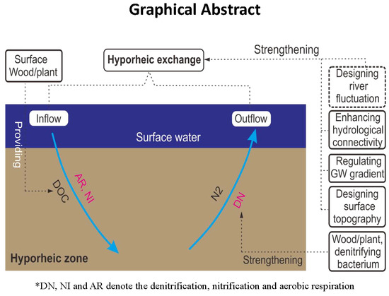
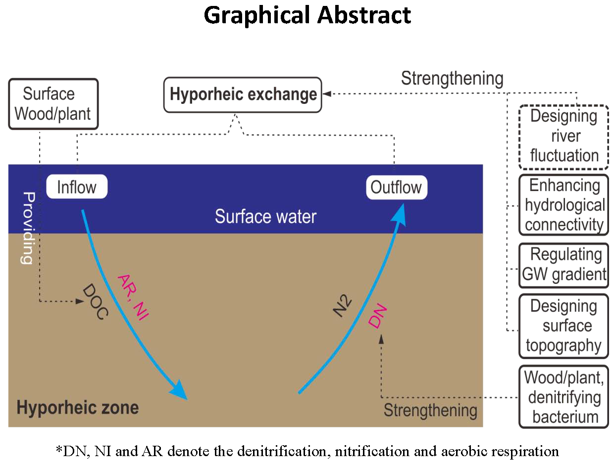
:Set in the downstream riparian zone of Xin’an River Dam, this paper established a 2D transversal coupling flow and solute transport and reaction model by verification within situ groundwater level and temperature. The denitrifying methods and principles in the riparian zone from the perspective of hyporheic exchange were explored, which provided a basis for the engineering techniques for river ecological restoration. Our studies have shown that under the condition of water level fluctuation, a biological method such as adding denitrifying bacteria biomass to a fixed degree (the same below) can greatly increase the denitrifying rate (1.52 g/d) in the riparian zone; chemical methods such as adding organic carbon into the surface water or groundwater can increase the total riparian nitrate removal (8.00–8.18 g) and its efficiency (19.5–20.0%) to a great extent; hydrogeological methods such as silt cleaning of the aquifer surface or local pumping around the contaminated area can increase the total riparian nitrate removal (1.06–14.8 g) to some extent, but correspondingly reduce the denitrifying efficiency (0.95–1.4%); physical methods such as designing the bank form into gentle slope or concave shape can slightly increase the total riparian nitrate removal (0.22–0.52 g) and correspondingly improve the denitrifying efficiency (0.25–0.85%). At the application level of river ecological restoration, integrated adopting the above methods can make the riparian denitrifying effect “fast and good”.
1. Introduction
In the natural hydrologic cycle, surface water and groundwater are not independent units, but an organic whole, that is, there is a good hydrological connectivity between them. As early as 1959, Orghidan et al. [1] realized the ecological significance of the interface between surface water and surrounding groundwater, and first proposed the concept of the Hyporheic Zone. Up to now, previous studies all over the world have carried out a mass of research on hyporheic zone in different research fields, and great progress has been made not only in the understanding of the hyporheic exchange mechanism but also in the development of numerical models, indoor and outdoor testing techniques [2]. With the maturity of hyporheic exchange theory, in recent years, more and more scholars have concerned themselves with the quantitative study of hydrochemical process in the hyporheic zone, of which the nitrogen cycle was a hot topic.
Compared with flat terrain, a fluctuating riverbed structure can better improve the denitrifying capacity in the hyporheic zone. The typical riverbed structures are dune structure [3], wood structure [4] and riffle-deep pool structure [5]. In addition, Hu et al. [6] further compared the influences of riverbed staircase structures with and without microtopography on nitrogen cycle in the hyporheic zone, and found that microtopography increases the hyporheic exchange intensity and produces a series of short immigration paths on the shallow layer of hyporheic zone, which has a relatively high oxygen content, thus promoting nitrification and inhibiting denitrification, and furthermore resulting in a decrease in the denitrifying capacity in the hyporheic zone. Compared with the terrain factor, the surface water fluctuation is generally better for the hyporheic nitrate removal. Numerical simulation studies from Gu et al. [7], Shuai et al. [8] and Trauth et al. [9] have concluded that the greater the surface water level fluctuates and the longer the water level duration is, the stronger the denitrifying capacity in the hyporheic zone is. Liu et al. [10] found that under the assumed fixed upstream flood volume, the hyporheic denitrifying capacity first increases and then decreases with the duration/amplitude ratio of water level fluctuation, while it increases logarithmically with the pulse frequency of water level fluctuation. This is of great significance for the ecological restoration of the riparian zone downstream of the reservoir. In addition, Shuai et al. [8] further explored the impacts of surface water–groundwater hydraulic gradient, aquifer hydraulic conductivity and aquifer dispersion coefficient on the hyporheic nitrate removal under the condition of water level fluctuation.
In addition to the aforementioned topography and hydrogeological factors, there are many biochemical factors influencing nitrogen cycle in the hyporheic zone, for example: (1) denitrifying bacteria. Adding denitrifying bacteria, like Thiobacillus denitrificans and Micrococcus denitrificans, can effectively accelerate the denitrifying process [11]. (2) Dissolved oxygen. Dissolved oxygen has an inhibitory effect on denitrification, and it is generally controlled at 1mg/L [12]. Duff and Triska [13] studied the effect of dissolved oxygen concentration on the nitrogen cycle and confirmed that the nitrogen cycle in the hyporheic zone is mainly based on the redox process of biological effect. (3) Organic carbon source. The electron donors (hydrogen donors) in the denitrification process are a variety of organic substrates (carbon sources). For example, if methanol is taken as an organic carbon source, not only can NO2-N and NO3-N be reduced, but also oxidative decomposition of organics can be promoted. In consideration of an additional consumption of dissolved oxygen for organic carbon source, the dosage of organic carbon is generally higher than that of NO3-N [7,14]. Hu et al. [6] pointed out that the increase of organic carbon concentration in surface water can effectively promote aerobic respiration and cause the attenuation of nitrification for the consumption of dissolved oxygen. However, due to the existence of microtopography, denitrification is basically unaffected.
In summary, the researches on nitrogen cycle in the hyporheic zone have made great achievements, but there are still some deficiencies. Firstly, although there have been some studies on the effects of chemical factors on surface–subsurface nitrogen flux [6], quantitative studies involving nitrogen transformation in the hyporheic zone are not sufficient, especially under the condition of water level fluctuation. Secondly, the researches on nitrogen cycle driven by the bank form are still insufficient, such as the effects of bank slope and concave and convex shapes on the riparian nitrogen cycle. Finally, there is still a lack of comparison among the impacts of the above mentioned hydrological, chemical and physical factors on the hyporheic denitrifying capacity.
In addition, although the hyporheic zone plays an unneglectable role in the maintenance of river ecological health, which has been gradually proved and accepted by the global community of scholars, the practice of incorporating the hyporheic zone into designing schemes and engineering measures for the ecological environment protection and restoration of the whole river is still lagging behind. The focus of many projects such as reservoir operation, aeration, aquatic plant restoration, sediment dredging, ecological revetment, constructed wetlands and chemical remediation are only limited to the surface water, while the hydrodynamic exchange process and ecological significance between surface water and nearby shallow groundwater are not considered, which makes them impossible for the river to maintain effective long-term self-purification capacity. Therefore, to coordinate and consider the basic elements of the river system and to carry out river ecological restoration from the perspective of hyporheic exchange should be one of the important contents of river ecological restoration and management.
Therefore, this paper discussed the influence principles of various factors on the hyporheic nitrate removal from the perspective of biochemistry, hydrogeology and topography. Under the premise of surface water fluctuation, the following aspects are discussed: (1) the impacts of denitrifying bacteria and dissolved organic carbon on the hyporheic denitrifying capacity, (2) the impacts of hydrological connectivity and surface water-groundwater hydraulic gradient on the hyporheic denitrifying capacity, and (3) the impacts of riverbank slope and convex and convex forms on the hyporheic denitrifying capacity. Furthermore, this paper narrated the corresponding feasible engineering measures, aiming at providing technical support for the current river restoration.
2. Methods
2.1. Study Site
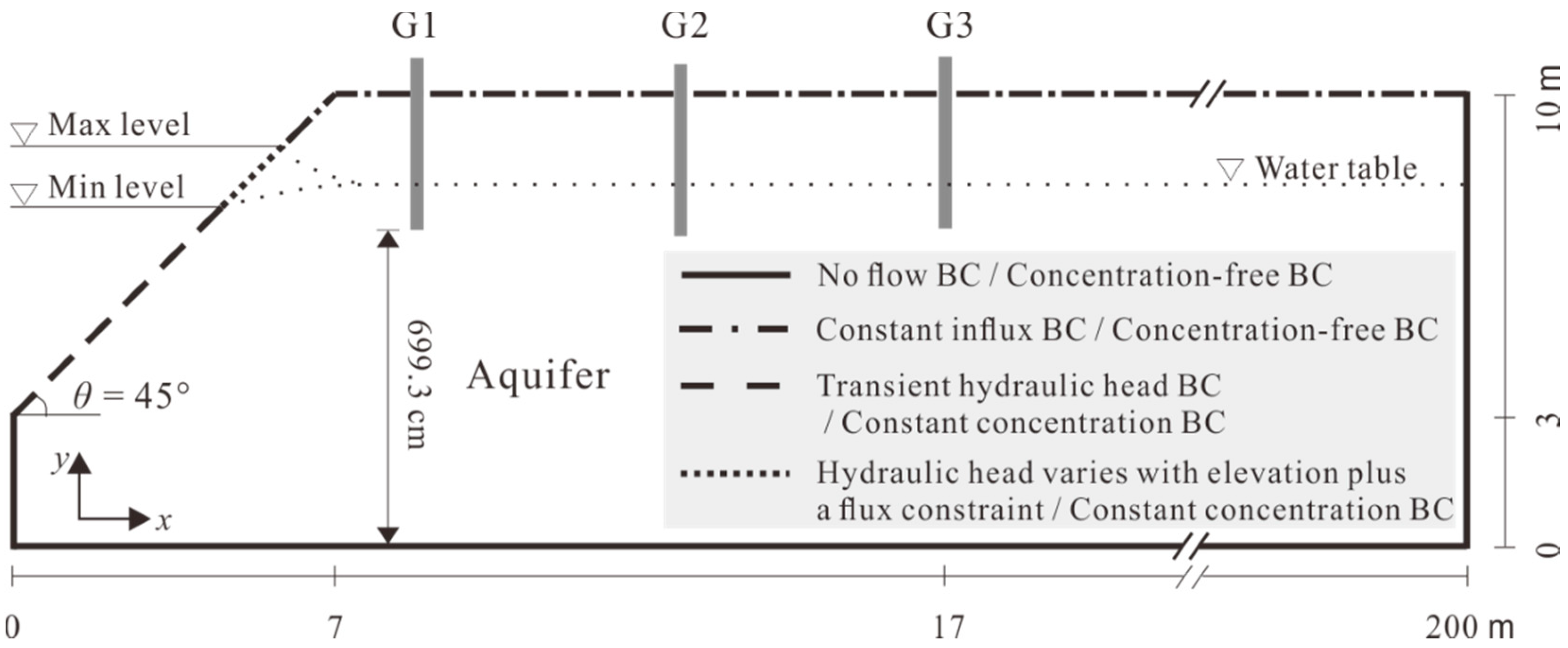
The field site is located in the riparian zone (29°24’ N, 119°21’ E) downstream of the Xin’an River Dam, Jiande, China (see [15] for details). The river water level at the site has been often affected by the upstream reservoir discharge for years, with the amplitude up to 1 m. Three water-level monitoring wells were arranged along the cross section of the riparian zone. The horizontal line 699.3 cm below the bottom of well #1 [15] was set as the baseline (i.e., 0 m). In each well an HM21 input liquid level transmitter that is accurate up to 0.1 cm was installed. The data were automatically recorded every 5 min through a real-time automatic acquisition system to the computer via a remote terminal. There was large amount of gravels in the riparian zone, of which the maximum gravel size exceeded 10 cm. Hence, it was inconvenient to conduct slug tests. By sampling the soil at different depths around the monitoring wells and conducting particle diameter analyses and indoor Darcy Penetration tests, the effective porosity of the aquifer was measured to be 0.4, and the average saturated hydraulic conductivity (K) was measured to be 137.2 m/day (Table 1).
2.2. Modeling
2.2.1. Conceptual Model
Based on the field tests, a two-dimensional cross-section coupling flow and solute transport and reaction model was constructed in the riparian zone. The domain was 200 m long and 10 m high, and the slope of the bank was 45° (Figure 1). The assumptions and simplifications of the model were the same as the model of Liu et al. [16]. The flow and chemical boundary conditions of the model were shown in Figure 1. Due to the lack of groundwater level data and the fact that groundwater level at the long distance from the river was nearly not affected by river fluctuation [17], the right boundary of the model was set as no flow boundary. The initial hydraulic head distribution of the study domain was obtained by steady simulation on a given type of boundary condition, while the initial concentration distribution of each solute was directly assigned according to the measurements.
2.2.2. Governing Equations
The model coupled the variable saturated flow [18] based on Richards’ Equation and solute transport and reaction process based on Advection–Dispersion–Reaction Equation (1). Richards’ Equation considered the poroelastic response of aquifer media that caused by changing hydrostatic loading, which was the same as that of previous studies [19,20,21].
where Cj is the concentration of solute j, mg/L; is the water content, -; q is the Darcy velocity vector, m/day; D is the hydrodynamic dispersion coefficient tensor, m2/day; is the reaction rate of solute j, mg/L/d.
Multicomponent reactions involved in the model included aerobic respiration (AR), nitrification (NI) and denitrification (DN). The organic matter (DOC) was represented by the chemical formula “CH2O”. All the reaction equations are as follows:
CH2O + O2→ H2O + CO2
NH4+ + 2O2→NO3−+ H2O + 2H+
5CH2O + 4NO3−+ 4H+→7H2O + 5CO2+ 2N2
By using the Multiple-Monod kinetics model to represent the aforementioned reactions [22], the reaction terms in Equation (1) are expressed as following:
where CO2, CNH4, CNO3 and CDOC (mg/L) are the concentrations of dissolved oxygen (O2), ammonium (NH4+), nitrate (NO3−) and dissolved organic carbon (DOC), respectively; RO2, RNH4, RNO3 and RDOC (mg/L/d) are the reaction rates of O2, NH4+, NO3− and DOC, respectively; VAR, VNT, VDN (1/d) are the maximum specific uptake rates of the substrate of AR, NT and DN, respectively; XAR, XNT and XDN (mg/L) are the biomass of the functional microbial groups of promoting AR, NT and DN, respectively; KO2, KNH4, KNO3 and KDOC (mg/L) are the half-saturation constants of O2, NH4+, NO3− and DOC, respectively; KI (mg/L) is the inhibition constant; yO2 (-) is the O2 partition coefficient; UAR, UNT and UDN (U = VX) (mg/L/d) are the lumped specific maximum microbial reaction rates of AR, NT and DN, respectively.
2.2.3. Numerical Model and Its Verification
The numerical modelling code FEFLOW 7.0 [23] was used to simulate the variably saturated flow and solute transport and reaction by using the PARDISO solver [24]. The model domain was discretized through triangular grid generator, with finer mesh (dx = 0.1 m) around the surface water–groundwater interface (0 < x < 20 m) and water-level sensors, medium mesh (dx = 0.5 m) within 20 < x < 100 m region and larger mesh (dx = 2 m) within 100 < x < 200 m region. The total number of model grid cells was 46,679, and the total number of nodes was 23767. In order to keep the computational time within reasonable limits, the automatic time-step control was adopted by setting the initial time step of 0.001d and maximum time step of 0.5d. The model was calibrated by mainly adjusting K through comparing the calculated and measured values of groundwater level and temperature, with the other flow and thermal parameters being the empirical values of sandy loam described by [25]. The calibration and verification periods were respectively 26 October–26 December 2014 and 1–21 October 2015. Due to the lack of observational nitrogen data, the solute transport and reaction model was not calibrated, and the biochemical parameters were assigned by empirical values too.
2.2.4. Quantification of Biogeochemical Reaction
Under the water level fluctuation, the consumption of solute j (Mrem-j, g) at any time can be obtained by the following:
where T is the simulation time, d; is the area of the study domain, m2.
The maximum infiltration of solute j into the aquifer (, g) is as follows:
where C0 is the initial concentration of solute j in surface water, mg/L; (d) is the infiltration time and q (m2/day) denotes the exchange flux between the surface water and groundwater that obtained by integrating the normal velocity (vn, m/day) along the stream–aquifer interface:
where l is the length of the stream–aquifer interface, m.
The consumption efficiency of solute j (, -) can be further calculated:
2.2.5. Model Scenarios
The verified model was used to study the nitrogen cycle in the riparian zone under the coexistence of water level fluctuation and other factors at the site. The amplitude and duration of the water level fluctuation are A = 0.6 m, T = 3 d, respectively. The initial groundwater level (7.74 m) was assigned of the average base flow water-level at the site from 2014 to 2015. This paper aims to explore the methods and principles of improving the denitrifying capacity in the riparian zone from many aspects. For example, biological method such as adding denitrifying bacteria into the aquifer; chemical methods include increasing DOC concentration of surface water and groundwater; hydrogeological methods include enhancing hydrological connectivity and initial surface water-groundwater hydraulic gradient; topography methods include changing the slope and concave and convex shapes of the bank. All the numerical test cases are shown in Table 2.
3. Results
3.1. Model Test
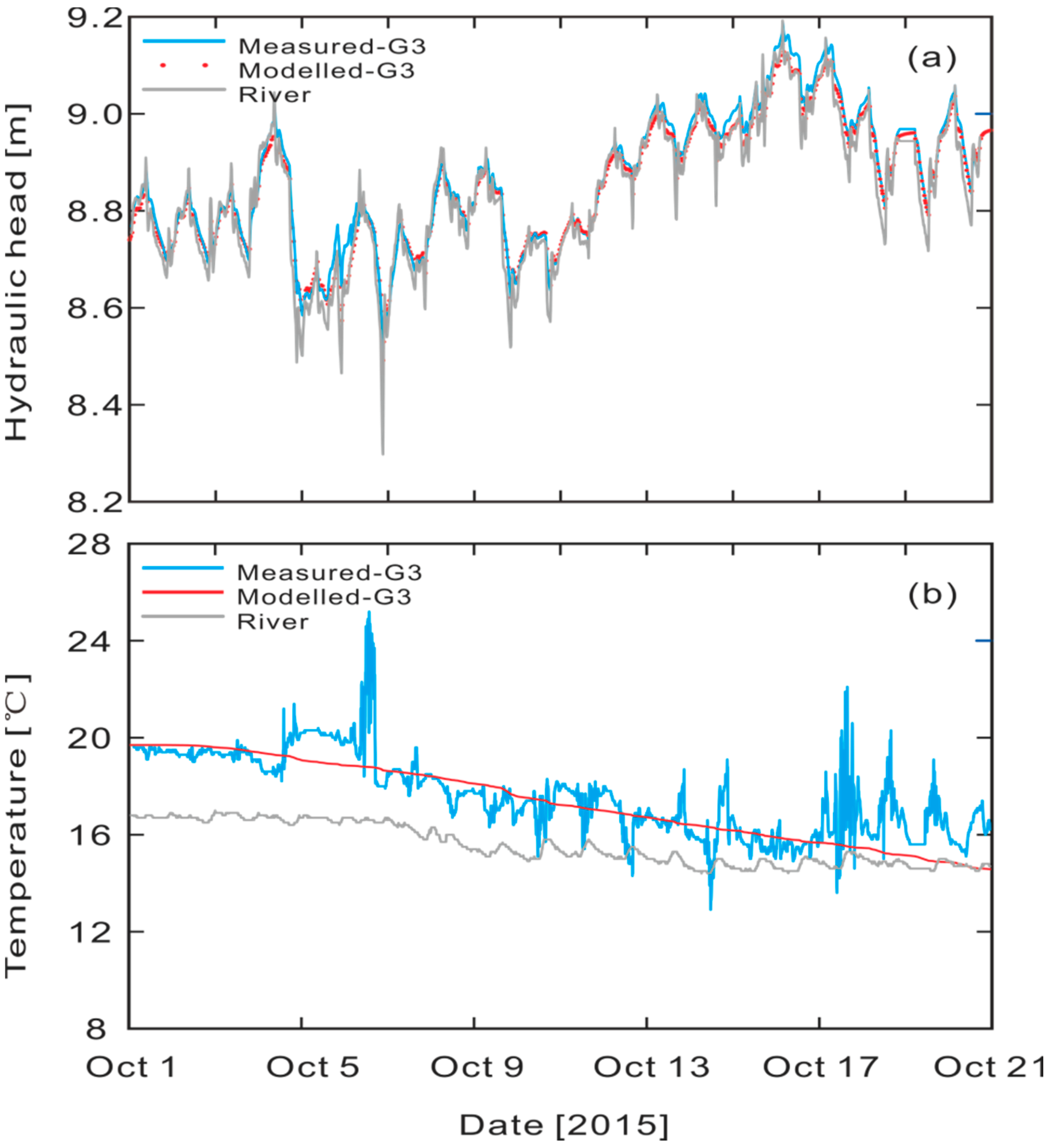
The numerical modelled and measured hydraulic heads were shown in Figure 2a. Overall, the assigned parameters were basically in line with the actual situation. The established numerical model could basically recreate the groundwater flow field at the site. The overall trend of modelled temperature was consistent with the measured values (Figure 2b). The reason for the fluctuation of measured temperature might be that the monitoring well was not sealed, resulting in the measured values being greatly affected by the air temperature. All the input parameters of the model are shown in Table 3. Since the aquifer contains a large amount of gravel, the longitudinal dispersity of the model was set to 1 m. Biochemical parameters were set according to the empirical values that obtained by comparing multiple literatures.
3.2. Biochemical Methods for Denitrifying
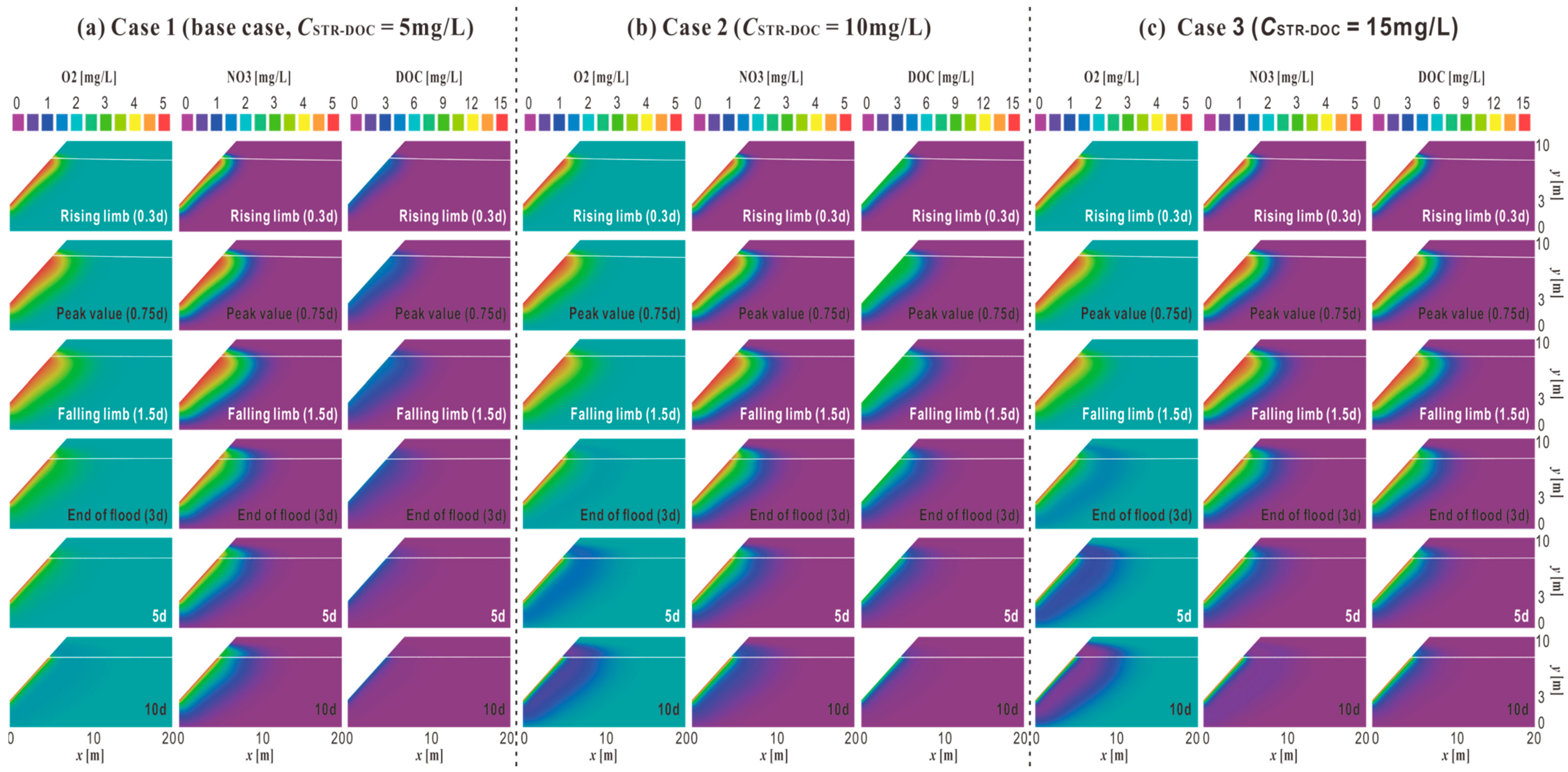
Figure 3 showed the concentration distribution of O2, NO3− and DOC at typical moments of water level fluctuation under the conditions of different surface water DOC concentrations. In the surface water infiltration period (t < 1.5 d), the concentration distribution of NO3− (or O2) was almost unchanged in all cases. It was because the dominant factor affecting the concentration distribution of each solute was its infiltration capacity from surface water; by comparison, the change of DOC concentration in surface water had relatively small impact on AR, NI and DN during this period, namely, the solute reactivity was much smaller than the infiltration capacity. During the groundwater backflow period (t > 1.5 d), the concentration distribution of NO3− (or O2) varied greatly under different cases, mainly due to the riparian zone no longer receiving the solute recharging from the surface water, and the chemical reaction was the dominant factor in the change of solute concentration distribution. Comparing the different cases in Figure 3, with the increase of DOC concentration in surface water, the NO3− plume shrunk obviously in the water level descending period, and the low-concentration-zone of O2 expanded significantly, which indicated that increasing the DOC concentration in surface water could strengthen the AR and DN and thereby enhance the denitrifying effect. During the whole water level cycle, when the DOC concentration of surface water increased from 5 mg/L to 15 mg/L (namely, raise twice), the denitrifying amount (Mrem-NO3) increased from 6.34 g to 22.70 g (namely, raise 2.6 times), correspondingly, the maximum denitrifying rate increased from 1.58 g/d to 3.39 g/d. Since the total amount of NO3− infiltrating into the riparian zone (Min-NO3 = 40.90 g) was a constant, the denitrifying efficiency (Nrem-NO3) increased from 15.5% to 55.5% (Table 4).
By comparing cases 4, 5 and 6, the AR and DN processes in the riparian zone were obviously enhanced with the increase of DOC concentration in groundwater, which was corroborated by the decrease of overall O2 concentration, significant increase of low-value area of DOC concentration and obvious shrink of the NO3− plume during the water level descending period (concentration distribution picture was omitted). During the water level cycle, when the groundwater DOC concentration increased from 0 mg/L to 10 mg/L, Min-NO3 increased from 6.34 g to 22.23 g, and the maximum denitrifying rate increased from 1.58 g/d to 4.89 g/d correspondingly. Min-NO3 = 40.90 g kept no change, resulting in Nrem-NO3 increased from 15.5% to 54.5% (Table 4). Thus, when the DOC concentration of surface water or groundwater increased to the same extent (10 mg/L), the increase of maximum denitrifying rate induced by surface water was smaller than that of groundwater (3.39 g/d < 4.89 g/d), but the final denitrifying amount was larger (22.70 g > 22.23 g). This was because that the increase of groundwater DOC concentration could ensure the riparian zone with a relatively high DOC concentration in a short time, thereby improving the denitrifying rate. However, the total DOC involved in the DN process was relatively small, resulting in a small denitrifying amount.
Denitrifying bacteria mainly affected the DN process, while it had little effect on AR. Comparing cases 7, 8 and 9, the DOC and NO3− plumes involved in the DN process decreased with the increase of XDN, while the O2 plume had no significant change (concentration distribution picture was omitted). During the water level cycle, when XDN increased from 2 mg/L to 6 mg/L, Mrem-NO3 increased from 6.34 g to 11.38 g, the maximum denitrifying rate increased from 1.58 g/d to 4.61 g/d correspondingly, while Min-NO3 = 40.90g kept no change, resulting in Nrem-NO3 increased from 15.5% to 27.8% (Table 4). When XDN increased 2 times, the denitrifying amount and maximum denitrifying rate increased about 5 g and 3 g/d, respectively. By comparison, when the surface water DOC concentration increased 2 times, the denitrifying amount and maximum denitrifying rate increased about 16 g and 1.8 g/d, respectively. Therefore, increasing XDN could speed up the denitrifying process, but the denitrifying process would be limited to the infiltration amount of DOC from the surface water, causing the denitrifying amount by increasing XDN was smaller than that by increasing the DOC concentration in surface or groundwater.
3.3. Hydrogeological Methods for Denitrifying
Figure 4 showed the concentration distribution of O2, NO3− and DOC at typical moments of water level fluctuation under different K. When the hydrological connectivity was enhanced, the AR and DN reaction areas were significantly enlarged, which was corroborated by that all the solute plumes increased with the increasing K at any moment during the water level cycle. In Table 5, the corresponding denitrifying amounts under different K were shown, which quantitatively indicated that the larger K was, the greater the denitrifying capacity was. This was because the better hydrological connectivity could increase the maximum aquifer water storage (Qmax) (Table 5), and Min-NO3 has positive correlation with Qmax [7]. During the water level cycle, when the K increased from 43.2 m/day to 129.6 m/day, Min-NO3 increased from 40.90 g to 66.75 g, the range of reaction (lateral coordinate) increased from x = 10 m to x = 12 m, Mrem-NO3 increased from 6.34 g to 8.46 g, the maximum denitrifying rate increased from 1.58 g/d to 2.57 g/d, while Nrem-NO3 decreased from 15.5% to 12.7% (Table 5).
By comparing cases 13, 14 and 15, the range of each solute plume increased with the increase of i. During the water level regression period, each solute plume did not shrink but continued expanding (concentration distribution picture was omitted), which indicated that the consumption of solute through chemical reactions was smaller than solute being carried from the river induced by the hydraulic gradient between surface water and groundwater. During the water level cycle, the range of reaction (lateral coordinate) increased from x = 10 m to x = 16 m, Mrem-NO3 increased from 6.34 g to 35.89 g, the maximum denitrifying rate increased from 1.58 g/d to 2.18 g/d, while Nrem-NO3 reduced from 5.5% to 13.6% (Table 5). It could be found that the maximum denitrifying rate had no significant change with the change of i, and the influence of i on Min-NO3, Mrem-NO3 and the reaction range were much greater than that of K on them.
3.4. Topography Methods for Denitrifying
By comparing cases 16, 17 and 18, the shapes of all the solute plumes were narrow and long when the bank form was gentle; conversely, the shapes of all the solute plumes were wide and short (concentration distribution picture was omitted). In general, the range of each solute plume (corresponding to reaction area) decreased with the increase of , which indicated that the larger the was, the weaker the AR and DN were, thereby the smaller the denitrifying amount was. This could be quantitatively explained from Table 6. During the water level cycle, when increased from 30° to 60°, Min-NO3 reduced from 42.30 g to 40.12 g, the reaction area (t = 1.5 d) reduced from 44.5 m2 to 43.7 m2, Mrem-NO3 reduced from 7.03 g to 6.00 g, the maximum denitrifying rate reduced from 1.64 g/d to 1.53 g/d, and Nrem-NO3 reduced from 6.6% to 14.9% (Table 6).
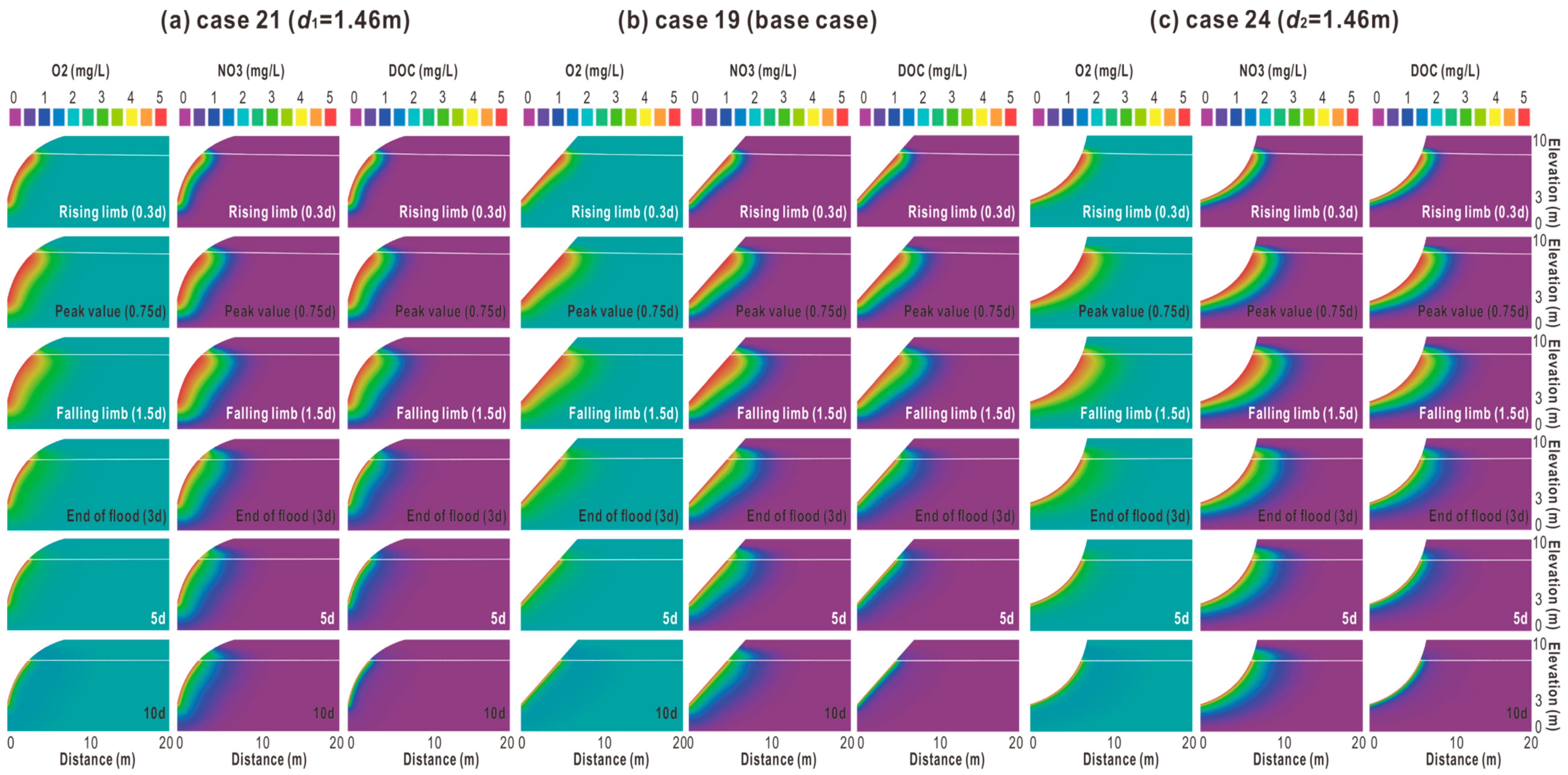
Figure 5 showed the concentration distribution of O2, NO3− and DOC at typical moments of water level fluctuation corresponding to the convex, flat, and concave bank form. When the bank form was convex, the shapes of all solute plumes were wide and short; while the bank was concave, the shapes of all solute plumes were narrow and long. In general, the range of each solute plume (corresponding to reaction area) in the convex bank was relatively small, while the corresponding reaction area in the concave bank was relatively large. It could be seen from Table 6 that the larger the convex distance was, the smaller the denitrifying amount was; conversely, the larger the concave distance was, the larger the denitrifying amount was. During the water level cycle, when d1 increased from 0 to 1.46 m, Min-NO3 decreased from 40.90 g to 39.38 g, Mrem-NO3 decreased from 6.34 g to 5.89 g, the corresponding maximum denitrifying rate decreased from 1.58 g/d to 1.50 g/d, and Nrem-NO3 reduced from 5.5% to 14.7% (Table 6). When d2 decreased from 0 to −1.46 m, Min-NO3 increased from 40.90 g to 42.31 g, Mrem-NO3 increased from 6.34 g to 6.77 g, the corresponding maximum denitrifying rate increased from 1.58 g/d to 1.63 g/d, and Nrem-NO3 increased from 5.5% to 16.1%. It could be found that if the bank form had the same extent of convex and concave, their weights of influence on the denitrifying capacity were almost the same.
4. Discussion
4.1. Deficiency of the Model
The two-dimensional, variably saturated, and multispecies reactive transport model in this paper has many shortcomings. First, the flow model was based on a series of assumptions, which could be seen for details from the model of [16]. Secondly, the calibration of the flow model was determined by mainly adjusting the hydraulic conductivity of the aquifer. Because the hydraulic conductivity was very sensitive to the model, and there were many deviations of the indoor Darcy Penetration tests in obtaining the hydraulic conductivity. Thirdly, the biogeochemical parameters of the model were set according to the empirical values as the previous studies [8], which had non-ignorable influences on the model results. Lastly, in the nitrogen cycle of the chemical model, process like anaerobic ammoxidation (DNRA) was not taken into consideration, which had a certain impact on the transformation of nitrogen [14]. In summary, the calculations of the denitrifying amount in the riparian zone of this model under various cases might be just estimated values, however it did not affect our exploration to the denitrifying methods and principles in the riparian zone of a regulated river.
4.2. Implications
4.2.1. Principles of Biochemical Denitrifying and Engineering Measures
In general, the influence principles of surface water and groundwater quality and denitrifying bacteria on riparian denitrifying amount were the same, that is to say, they all increased the denitrifying capacity by enhancing chemical reactivity. However, there were some differences. Increasing DOC concentration of surface water and groundwater improved the denitrifying capacity by increasing the electronic donors in the denitrification process, while increasing denitrifying bacteria biomass was equivalent to the catalyst function on denitrification. Therefore, the formers had greater impacts on the denitrifying amount in the riparian zone, while the latter mainly had a greater impact on the denitrifying rate.
Hence, in the heavy nitrate contaminated riparian zone, appropriate waste wood materials can be piled up at the interface between surface water and groundwater according to local conditions, which can be provided as the carbon source for DOC being infiltrated into the aquifer from surface water, thereby promoting the removal of nitrogen. Furthermore, some tree branches and leaves can be put or some green plants can be planted on the surface of the riparian zone, so that the rain will carry a certain amount of DOC into the aquifer to increase the groundwater DOC concentration and promote the removal of nitrogen. In addition, mycobacterium szulgai and pseudomonas fluorescens can be directly put into the aquifer to increase the biomass concentration of denitrifying bacteria. This method cannot greatly increase the denitrifying amount in the riparian zone, but it can effectively speed up the denitrifying process and improve the denitrifying efficiency.
4.2.2. Principles of Hydrogeological Denitrifying and Engineering Measures
The influence principle of K or i on the riparian denitrifying amount was different from that of the biochemical factors. The latter increased the riparian denitrifying amount by enhancing the chemical reactivity, while the former increased the denitrifying amount by enhancing the hyporheic exchange and increasing the total amount of solute infiltration. Compared with the previous studies [8], the influences of K and i on Min-NO3, Mrem-NO3 and Nrem- NO3 are the same, which also indicates the rationality of this model. In addition, although increasing K or i could increase Mrem-NO3 to some extent, but Nrem-NO3 was decreased correspondingly. This is because that Nrem-NO3 is the ratio of Mrem-NO3 to Min-NO3. When K or i increased, the increase extent of numerator was smaller than denominator. For example, Min-NO3 = 5g and the corresponding Mrem-NO3 = 2 g, then Nrem-NO3 = 40%. Increasing K to make Min-NO3 be 10 g, and assuming 10 g is the sum of the total infiltration in two periods. During the previous period, NO3− infiltration amount is 5 g and the corresponding Mrem-NO3 is 2 g. During the latter period, NO3− infiltration amount is also 5 g, but the corresponding Mrem-NO3 is less than 2 g. This is because the concentration of DOC in the riparian zone is lower than that of O2 after the asymmetric chemical reaction in the previous period (nitrification consumes less O2 while denitrification consumes more DOC), causing O2 being relatively surplus in the latter period, thereby inhibiting the denitrification to a certain extent. Therefore, the total denitrifying amount becomes smaller (<4 g), and finally Nrem-NO3 becomes smaller overall (<40%).
In practical measures, K can be increased by clearing the sedimentary silt along the interface between river and bank. In general, the hydraulic conductivity of the silt in aquifer surface is about two orders of magnitude lower than that of the aquifer. Hence, silt cleaning will greatly increase the hyporheic exchange during the water level fluctuation and improve the riparian denitrifying capacity correspondingly. As for the increase of i, it can be achieved by local pumping measures in the bank. In order to reduce the workload, local underground pumping can be carried out near the seriously contaminated riparian zone.
4.2.3. Principles of Topography Denitrifying and Engineering Measures
The influence principle of the bank form on the riparian denitrifying capacity during the water level fluctuation was basically the same as K or i, all of them increased Min-NO3 and Mrem-NO3 by enhancing the hyporheic exchange. However, the bank form was a factor that influenced the hyporheic exchange by influencing the exchange scope, while K or i was a factor that influenced the hyporheic exchange by influencing the exchange intensity. This result has been proved by the previous studies [17]. The influence principles of the bank forms such as bank slope, concave and convex shape on the riparian denitrifying capacity were similar. The convex bank essentially had the same effect on the riparian denitrifying capacity as the increase of the bank slope, both of which reduced the length of the river–bank interface and thus reduced the scope of hyporheic exchange, thereby resulting in the corresponding decrease of Qmax, Min-NO3 and Mrem-NO3. Similarly, when the bank was concave, it had the same effect as the decrease of the bank slope, resulting in the increase of Mrem-NO3. Comparing the impacts of bank forms with that of the above biochemical and hydrogeological factors on riparian denitrifying capability, it could be found that the influence degree of changing bank form on the riparian denitrifying capability was relatively much smaller. This is due to the little effect of changing bank form on the hydrodynamic exchange between surface water groundwater, which results in a small amount of the solute infiltration.
Comparing to the concave or convex shape, the bank slope has a relatively greater impact on the riparian denitrifying capacity, but it has some limitations in the application of engineering measures. It is impossible to make the bank slope unrestrictedly small, so in practical applications, the bank can be designed as a gentle slope with a concave shape, which will improve the riparian denitrifying capacity in a good way. The previous studies [3] have shown that riverbed dune morphology has a positive impact on the vertical hyporheic exchange and hyporheic denitrifying effect. Therefore, this paper has also calculated and compared the denitrifying capacity in the riparian zone with flat and undulated bank (calculation process omitted). However, the undulating shape of the bank had no obvious effect on the riparian denitrifying capacity. The possible reason is that a bank form with a certain undulating shape is equivalent to the combination of a series of concave and convex shapes. As mentioned above, the effect of the concave and convex shape of the bank on the riparian denitrifying capacity was opposite, which made the undulating shape of the bank have a mutual offset on riparian denitrifying capacity.
5. Conclusions
The main conclusions were summarized as follows:
- (1)
- Increasing the DOC concentration of surface water and groundwater could largely increase the denitrifying amount in the riparian zone and accordingly increase the denitrifying efficiency. By comparison, adding denitrifying bacteria biomass had a smaller impact on the denitrifying amount, but it could improve the denitrifying rate to a great extent. The combined applications of these methods can make the denitrifying effect in the riparian zone “fast and good”.
- (2)
- Enhancing the hydrological connectivity of the aquifer surface could increase the denitrifying amount in the riparian zone to a certain extent, but the denitrifying efficiency was reduced correspondingly. By comparison, increasing the surface–groundwater hydraulic gradient had a much greater impact on the denitrifying amount, with the denitrifying efficiency reducing too. In practical applications, pumping the groundwater in the heavily polluted reach and cleaning the surface sedimentary sludge can effectively improve the denitrifying capacity in the riparian zone.
- (3)
- Designing the bank form into a concave shape could slightly increase the denitrifying amount in the riparian zone and correspondingly improve the denitrifying efficiency. By comparison, reducing the bank slope could largely increase the denitrifying amount and also improve the denitrifying efficiency. In practical applications, designing the bank form into a gentle slope with concave shape can improve the denitrifying capacity in the riparian zone to a certain extent.
Author Contributions
We are grateful to the three anonymous reviewers. Conceptualization, D.L. and J.Z.; methodology, D.L.; software, H.Z.; validation, D.L., B.Z. and J.Z.; formal analysis, D.L.; investigation, H.Z.; resources, D.L.; data curation, H.Z.; writing—original draft preparation, D.L.; writing—review and editing, J.Z.; visualization, B.Z.; supervision, D.L.; project administration, J.Z.; All authors have read and agreed to the published version of the manuscript.
Funding
This work is funded by the Natural Science Foundation of China (51279045) and partly funded by the key projects of NHRI (No. Y919005, No. Y920012) and 66th China Postdoctoral Science Foundation (2019M661882).
Acknowledgments
Helmholtz Centre for Environmental Research–UFZ is acknowledged for providing a free license for FEFLOW 7.0. The data that support the findings of this study are available from the authors, including the measured and modelled water level and temperature and some concentration distributions not provided in the manuscript, which can be seen in the following links (extraction code: mtzc): https://pan.baidu.com/s/1zchXqUTZ8risA5y1fUG4eg. The data of Min-NO3, Mrem- NO3 and Nrem-NO3 in each case are not included because they are processed by the model and shown in Tables.
Conflicts of Interest
The authors declare no conflict of interest.
References
- Orghidan, T. Einneuer Lebensraum des unterirdischen Wassers: Der hyporheischeBiotop. Arch. Hydrobiol. 1959, 55, 392–414. [Google Scholar]
- Xia, J.; Chen, Y.; Wang, W.; Han, Y.; Liu, H.; Hu, L. Dynamic processes and ecological restoration of hyporheic layer in riparian zone. Adv. Water Sci. 2013, 24, 1–10. [Google Scholar]
- Bardini, L.; Boano, F.; Cardenas, M.B.; Revelli, R.; Ridolfi, L. Nutrient cycling in bedform induced hyporheic zones. Geochim. Cosmochim. Acta 2012, 84, 47–61. [Google Scholar] [CrossRef] [Green Version]
- Cardenas, M.B. Stream-aquifer interactions and hyporheic exchange in gaining and losing sinuous streams. Water Resour. Res. 2009, 45, 267–272. [Google Scholar] [CrossRef]
- Daniele, T.; Buffington, J.M. Hyporheic exchange in gravel bed rivers with pool-riffle morphology: Laboratory experiments and three-dimensional modeling. Water Resour. Res. 2007, 430, 208–214. [Google Scholar]
- Hu, H.; Binley, A.; Heppell, C.M.; Lansdown, K.; Mao, X. Impact of microforms on nitrate transport at the groundwater-surface water interface in gaining streams. Adv. Water Resour. 2014, 73, 185–197. [Google Scholar] [CrossRef]
- Gu, C.; Anderson, W.; Maggi, F. Riparian biogeochemical hot moments induced by stream fluctuations. Water Resour. Res. 2012, 48, W09546. [Google Scholar] [CrossRef] [Green Version]
- Shuai, P.; Cardenas, M.B.; Knappett, P.S.K.; Bennett, P.C.; Neilson, B.T. Denitrification in the banks of fluctuating rivers: The effects of river stage amplitude, sediment hydraulic conductivity and dispersivity, and ambient groundwater flow. Water Resour. Res. 2017, 53, 7951–7967. [Google Scholar] [CrossRef]
- Trauth, N.; Musolff, A.; Knöller, K.; Kaden, U.S.; Keller, T.; Werban, U. River water infiltration enhances denitrification efficiency in riparian groundwater. Water Res. 2017, 130, 185–199. [Google Scholar] [CrossRef]
- Liu, D. Hyporheic Exchange and Solute Transport and Transformation Driven by Flood Wave; Hohai University: Nanjing, China, 2019. [Google Scholar]
- Hou, L.; Yin, G.; Liu, M.; Zhou, J.; Zheng, Y.; Gao, J.; Tong, C. Effects of sulfamethazine on denitrification and the associated N2O release in estuarine and coastal sediments. Environ. Sci. Technol. 2014, 49, 326–333. [Google Scholar] [CrossRef]
- Zhang, L.; Wang, S.; Wu, Z. Coupling effect of pH and dissolved oxygen in water column on nitrogen release at water-sediment interface of Erhai Lake, China. Estuar. Coast. Shelf Sci. 2014, 149, 178–186. [Google Scholar] [CrossRef]
- Duff, J.H.; Triska, F.J. Denitrification in sediments from the hyporheic zone adjacent to a small forested stream. Can. J. Fish. Aquat. Sci. 2011, 47, 1140–1147. [Google Scholar] [CrossRef]
- Zarnetske, J.P.; Haggerty, R.; Wondzell, S.M.; Bokil, V.A.; González-Pinzón, R. Coupled transport and reaction kinetics control the nitrate source-sink function of hyporheic zones. Water Resour. Res. 2012, 48, W11508. [Google Scholar]
- Liu, D.; Zhao, J.; Chen, X.; Li, Y.; Feng, M. Dynamic processes of hyporheic exchange and temperature distribution in the riparian zone in response to dam-induced water fluctuations. Geosci. J. 2018, 22, 1–11. [Google Scholar] [CrossRef]
- Liu, D.; Zhao, J.; Jeon, W.H.; Lee, J.Y. Solute dynamics across the stream-to-riparian continuum under different flood waves. Hydrol. Process. 2019, 33, 2627–2641. [Google Scholar] [CrossRef]
- Siergieiev, D.; Ehlert, L.; Reimann, T.; Lundberg, A.; Liedl, R. Modelling hyporheic processes for regulated rivers under transient hydrological and hydrogeological conditions. Hydrol. Earth Syst. Sci. 2015, 19, 329–340. [Google Scholar] [CrossRef] [Green Version]
- Voss, C.I. A finite element simulation model for saturated-unsaturated, fluid-density-dependent groundwater flow with energy transport or chemically reactive single-species solute transport. Water Resour. Investig. Rep. (USA) 1984, 84, 4369. [Google Scholar]
- Reeves, H.W.; Thibodeau, P.M.; Underwood, R.G.; Gardner, L.R. Incorporation of total stress changes into the ground water model SUTRA. Groundwater 2000, 38, 89–98. [Google Scholar] [CrossRef]
- Gardner, L.R.; Wilson, A.M. Comparison of four numerical models for simulating seepage from salt marsh sediments. Estuar. Coast. Shelf Sci. 2006, 69, 427–437. [Google Scholar] [CrossRef]
- Boutt, D.F. Poroelastic loading of an aquifer due to upstream dam releases. Groundwater 2010, 48, 580–592. [Google Scholar] [CrossRef]
- Molz, F.J.; Widdowson, M.A.; Benefield, L.D. Simulation of microbial growth dynamics coupled to nutrient and oxygen transport in porous media. Water Resour. Res. 1986, 22, 1207–1216. [Google Scholar] [CrossRef]
- Diersch, H.J. Finite Element Modeling of Flow, Mass and Heat Transport in Porous and Fractured Media; Springer: Berlin, Germany, 2014; p. 996. [Google Scholar]
- Schenk, O.; Gärtner, K. Solving unsymmetric sparse systems of linear equations with pardiso. Future Gener. Comput. Syst. 2004, 20, 475–487. [Google Scholar] [CrossRef]
- Carsel, R.F.; Parrish, R.S. Developing joint probability distributions of soil water retention characteristics. Water Resour. Res. 1988, 24, 755–769. [Google Scholar] [CrossRef] [Green Version]
- Fetter, C. Applied Hydrogeology, 4th ed.; Prentice Hall: Upper Saddle River, NJ, USA, 2000; p. 598. [Google Scholar]
- Schulze-Makuch, D. Longitudinal dispersivity data and implications for scaling behavior. Groundwater 2005, 43, 443–456. [Google Scholar] [CrossRef] [PubMed]
- Lee, M.S.; Lee, K.K.; Hyun, Y.; Clement, T.P.; Hamilton, D. Nitrogen transformation and transport modeling in groundwater aquifers. Ecol. Model. 2006, 192, 143–159. [Google Scholar] [CrossRef] [Green Version]
Figure 1.
A transversal 2D conceptual model of the riparian zone downstream of Xin’an River Dam. G1, G2 and G3 respectively represent water-level monitoring wells. Flow from left to right is defined as positive, and vice versa.
Figure 1.
A transversal 2D conceptual model of the riparian zone downstream of Xin’an River Dam. G1, G2 and G3 respectively represent water-level monitoring wells. Flow from left to right is defined as positive, and vice versa.

Figure 2.
The comparison between the measured and modelled hydraulic heads (a) and water temperature (b).
Figure 2.
The comparison between the measured and modelled hydraulic heads (a) and water temperature (b).

Figure 3.
The effect of surface water dissolved organic carbon (DOC) concentration on riparian nitrogen cycle driven by water level fluctuation. The white lines represent groundwater levels. CSTR-DOC denotes the DOC concentration of surface water.
Figure 3.
The effect of surface water dissolved organic carbon (DOC) concentration on riparian nitrogen cycle driven by water level fluctuation. The white lines represent groundwater levels. CSTR-DOC denotes the DOC concentration of surface water.

Figure 4.
The effect of hydrological connectivity on riparian nitrogen cycle driven by water level fluctuation. The white lines represent groundwater levels. K denotes the hydraulic conductivity of the saturated zone.
Figure 4.
The effect of hydrological connectivity on riparian nitrogen cycle driven by water level fluctuation. The white lines represent groundwater levels. K denotes the hydraulic conductivity of the saturated zone.

Figure 5.
The effect of different bank forms on riparian nitrogen cycle driven by water level fluctuation. The white lines represent groundwater levels. d1 and d2 denote the convex and concave distance, respectively.
Figure 5.
The effect of different bank forms on riparian nitrogen cycle driven by water level fluctuation. The white lines represent groundwater levels. d1 and d2 denote the convex and concave distance, respectively.


Table 1.
Hydraulic conductivity of unconfined aquifer in riparian zone.
| Method | Particle Diameter Analysis (Hazen Method) | Indoor Darcy Penetration Test | ||||
|---|---|---|---|---|---|---|
| 1 | 2 | 3 | 1 | 2 | 3 | |
| Hydraulic conductivity (m/day) | 228.1 | 113.2 | 169.3 | 104.5 | 88.1 | 120.1 |
Table 2.
The numerical test cases.
| Case | DOC Concentration of Surface Water (CSTR-DOC, mg/L) | DOC Concentration of Groundwater (CGW-DOC, mg/L) | Biomass Concentration of Denitrifying Bacteria (XDN, mg/L) | Hydraulic Conductivity of Saturated Aquifer (K, m/day) | Surface Water–Groundwater Hydraulic Gradient (i, -) | Bank Slope (, °) | Convex Distance (d1, m) | Concave Distance (d2, m) |
|---|---|---|---|---|---|---|---|---|
| 1 | 5 | 0 | 1 | 43.2 | 0 | 45 | 0 | 0 |
| 2 | 10 | 0 | 1 | 43.2 | 0 | 45 | 0 | 0 |
| 3 | 15 | 0 | 1 | 43.2 | 0 | 45 | 0 | 0 |
| 4 | 5 | 0 | 1 | 43.2 | 0 | 45 | 0 | 0 |
| 5 | 5 | 5 | 1 | 43.2 | 0 | 45 | 0 | 0 |
| 6 | 5 | 10 | 1 | 43.2 | 0 | 45 | 0 | 0 |
| 7 | 5 | 0 | 1 | 43.2 | 0 | 45 | 0 | 0 |
| 8 | 5 | 0 | 2 | 43.2 | 0 | 45 | 0 | 0 |
| 9 | 5 | 0 | 4 | 43.2 | 0 | 45 | 0 | 0 |
| 10 | 5 | 0 | 1 | 43.2 | 0 | 45 | 0 | 0 |
| 11 | 5 | 0 | 1 | 86.4 | 0 | 45 | 0 | 0 |
| 12 | 5 | 0 | 1 | 129.6 | 0 | 45 | 0 | 0 |
| 13 | 5 | 0 | 1 | 43.2 | 0 | 45 | 0 | 0 |
| 14 | 5 | 0 | 1 | 43.2 | 0.0025 | 45 | 0 | 0 |
| 15 | 5 | 0 | 1 | 43.2 | 0.005 | 45 | 0 | 0 |
| 16 | 5 | 0 | 1 | 43.2 | 0 | 30 | 0 | 0 |
| 17 | 5 | 0 | 1 | 43.2 | 0 | 45 | 0 | 0 |
| 18 | 5 | 0 | 1 | 43.2 | 0 | 60 | 0 | 0 |
| 19 | 5 | 0 | 1 | 43.2 | 0 | 45 | 0 | - |
| 20 | 5 | 0 | 1 | 43.2 | 0 | 45 | 0.73 | - |
| 21 | 5 | 0 | 1 | 43.2 | 0 | 45 | 1.46 | - |
| 22 | 5 | 0 | 1 | 43.2 | 0 | 45 | - | 0 |
| 23 | 5 | 0 | 1 | 43.2 | 0 | 45 | - | −0.73 |
| 24 | 5 | 0 | 1 | 43.2 | 0 | 45 | - | −1.46 |
Case 1, 4, 7, 10, 13, 17, 19 or 22 represents the base case, the other cases are generated by changing one parameter at a time and keeping the others constant.
Table 3.
The input parameters of the model (base case).
| Parameters | Input Values | Units |
|---|---|---|
| Flow parameters | ||
| Hydraulic conductivity of the saturated zone (K) a | 43.2 | m/day |
| Effective porosity (ne) a | 0.4 | - |
| Specific storage (S0) b | 0.0001 | 1/m |
| Residual saturation (sr) b | 0.15 | - |
| Maximum saturation (ss) b | 1 | - |
| The parameter of VG model () b | 7 | 1/m |
| The parameter of VG model (n) b | 1.89 | - |
| Longitudinal dispersivity (DL) c | 1 | m |
| Transverse/longitudinal dispersivity (DT/DL) c | 0.1 | - |
| Solute and biogeochemical parameters | ||
| The O2 concentration of surface water a | 5 | mg/L |
| The NH4+ concentration of surface water d | 0.05 | mg/L |
| The NO3− concentration of surface water d | 5 | mg/L |
| The DOC concentration of surface water a | 5 | mg/L |
| The NH4+ and NO3− concentration of groundwater d | 0 | mg/L |
| The DOC concentration of groundwater a | 0 | mg/L |
| The O2 concentration of groundwater a | 2 | mg/L |
| Maximum specific uptake rate for AR (UAR) e,f,g | 2 | mg/L/d |
| Maximum specific uptake rate for NI (UNI) e | 1.05 | mg/L/d |
| Maximum specific uptake rate for DN (UDN) e,f,g | 2 | mg/L/d |
| Half saturation constant for O2 (KO2) e,f,g | 1 | mg/L |
| Half saturation constant for NH4+ (KNH4) e,f | 0.5 | mg/L |
| Half saturation constant for NO3− (KNO3) e,f,g | 1 | mg/L |
| Half saturation constant for DOC (KDOC) e,f,g | 5 | mg/L |
| O2 inhibition constant (KI) e,f | 1 | mg/L |
| O2 partition coefficient (yO2) e | 0.64 | - |
Table 4.
Min-NO3, Mrem-NO3 and Nrem-NO3 under different biochemical cases.
| Case | CSTR-DOC (mg/L) | CGW-DOC (mg/L) | XDN (mg/L) | Min-NO3 (g) | Mrem-NO3 (g) | Nrem-NO3 (-) |
|---|---|---|---|---|---|---|
| 1 | 5 | 0 | 1 | 40.90 | 6.34 | 15.5% |
| 2 | 10 | 0 | 1 | 40.90 | 16.36 | 40.0% |
| 3 | 15 | 0 | 1 | 40.90 | 22.70 | 55.5% |
| 4 | 5 | 0 | 1 | 40.90 | 6.34 | 15.5% |
| 5 | 5 | 5 | 1 | 40.90 | 19.01 | 46.5% |
| 6 | 5 | 10 | 1 | 40.90 | 22.23 | 54.5% |
| 7 | 5 | 0 | 1 | 40.90 | 6.34 | 15.5% |
| 8 | 5 | 0 | 2 | 40.90 | 9.41 | 23.0% |
| 9 | 5 | 0 | 4 | 40.90 | 11.38 | 27.8% |
Min-NO3. Mrem-NO3 and Nrem-NO3 denote the maximum infiltration, consumption, and consumption efficiency of NO3−. Other symbols have the same meanings as Table 2.
Table 5.
Qmax, Min-NO3, Mrem-NO3 and Nrem-NO3 under different hydrogeological cases.
| Case | K (m/day) | i (-) | Qmax (m2) | Min-NO3 (g) | Mrem-NO3 (g) | Nrem-NO3 (-) |
|---|---|---|---|---|---|---|
| 10 | 43.2 | 0 | 6.2 | 40.90 | 6.34 | 15.5% |
| 11 | 86.4 | 0 | 9.0 | 55.67 | 7.56 | 13.6% |
| 12 | 129.6 | 0 | 11.1 | 66.75 | 8.46 | 12.7% |
| 13 | 43.2 | 0 | 6.2 | 40.90 | 6.34 | 15.5% |
| 14 | 43.2 | 0.0025 | 26.5 | 144.71 | 21.27 | 14.7% |
| 15 | 43.2 | 0.005 | 50.3 | 263.92 | 35.89 | 13.6% |
Qmax denotes the maximum aquifer water storage; Min-NO3, Mrem-NO3 and Nrem-NO3 denote the maximum infiltration, consumption and consumption efficiency of NO3−. Other symbols have the same meanings as in Table 2.
Table 6.
Qmax, Min-NO3, Mrem-NO3 and Nrem-NO3 under different topography cases.
| Case | (°) | d1 (m) | d2 (m) | Qmax (m2) | Min-NO3 (g) | Mrem-NO3 (g) | Nrem-NO3 (-) |
|---|---|---|---|---|---|---|---|
| 16 | 30 | 0 | 0 | 6.23 | 42.30 | 7.03 | 16.6% |
| 17 | 45 | 0 | 0 | 6.20 | 40.90 | 6.34 | 15.5% |
| 18 | 60 | 0 | 0 | 6.07 | 40.12 | 6.00 | 14.9% |
| 19 | 45 | 0 | - | 6.20 | 40.90 | 6.34 | 15.5% |
| 20 | 45 | 0.73 | - | 6.16 | 40.23 | 6.12 | 15.2% |
| 21 | 45 | 1.46 | - | 6.11 | 39.38 | 5.89 | 14.7% |
| 22 | 45 | - | 0 | 6.20 | 40.90 | 6.34 | 15.5% |
| 23 | 45 | - | −0.73 | 6.22 | 41.91 | 6.60 | 15.7% |
| 24 | 45 | - | −1.46 | 6.24 | 42.31 | 6.77 | 16.0% |
Qmax denotes the maximum aquifer water storage; Min-NO3, Mrem-NO3 and Nrem-NO3 denote the maximum infiltration, consumption and consumption efficiency of NO3−. Other symbols have the same meanings as in Table 2.
© 2020 by the authors. Licensee MDPI, Basel, Switzerland. This article is an open access article distributed under the terms and conditions of the Creative Commons Attribution (CC BY) license (http://creativecommons.org/licenses/by/4.0/).
Share and Cite
MDPI and ACS Style
Liu, D.; Zhu, B.; Zhu, H.; Zhao, J. Feasible Ways Promoting Nitrate Removal in Riparian Zone Downstream of a Regulated River. Water 2020, 12, 2054. https://0-doi-org.brum.beds.ac.uk/10.3390/w12072054
AMA Style
Liu D, Zhu B, Zhu H, Zhao J. Feasible Ways Promoting Nitrate Removal in Riparian Zone Downstream of a Regulated River. Water. 2020; 12(7):2054. https://0-doi-org.brum.beds.ac.uk/10.3390/w12072054
Chicago/Turabian StyleLiu, Dongsheng, Bei Zhu, Haoyu Zhu, and Jian Zhao. 2020. "Feasible Ways Promoting Nitrate Removal in Riparian Zone Downstream of a Regulated River" Water 12, no. 7: 2054. https://0-doi-org.brum.beds.ac.uk/10.3390/w12072054
Note that from the first issue of 2016, this journal uses article numbers instead of page numbers. See further details here.