1. Introduction
As one of the most widespread natural process in mountainous environments, the occurrence of debris flow events often poses significant damage and a threat to infrastructure, urban development, and the livelihood of humans, even potentially resulting in loss of life [
1,
2,
3]. With rapid socio-economic development, this situation tends to be more critical, particularly if it is not well handled. In this case, relevant studies in these popular research areas have been the focus of many researchers. However, owing to the predisposing and triggering factors of this natural phenomenon, the total control of debris flow events is always difficult, transforming the focus of contemporary studies from reducing the occurrence of debris flow to predicting its spatial and temporal occurrence. With the advanced prediction of this hazard, the damage and threat caused by this phenomenon may easily be mitigated and/or avoided completely.
Currently, many studies focus on thoroughly determining the susceptibility to representing the likelihood of debris flow occurrence. In these studies, the heuristic and probabilistic models are widely used. The main postulation of these models is on the thought adopted from the principle that “the past and present are keys to the future” [
4], i.e., the area where debris flow has occurred in the past is most likely to be affected by the same event in the future. It also means that areas with conditions similar to those that have already been affected by debris flow are more prone to further debris flow events [
5,
6,
7]. These models estimate the probability of debris flow occurrence by analyzing the relationship between debris flow incidents and existing geo-environmental factors [
8,
9]. For instance, a study by Kritikos and Davies [
10] applied a data-driven fuzzy membership model to assess the susceptibility of debris flow in the Southern Alps in southwestern New Zealand. Cama and Lombardo [
11] adopted a binary logistic regression model to estimate the susceptibility of debris flow in Messina, Italy. Furthermore, a considerable number of studies have been performed using heuristic or probabilistic models to assess the susceptibility of debris flow [
12,
13,
14]. Despite the differences in the approach used, each model requires an accurate, reasonable, and complete catalog of historical debris flow events [
15], and the support of detailed and sufficient environmental data to make the results relatively objective and reproducible. Consequently, these models are commonly considered to constitute the most appropriate approach at large or medium scales [
16,
17]. However, one of the greatest limitations of these models is that acquiring accurate and complete historical records and detailed data, which is the key to suitable susceptibility assessment, is often difficult to obtain [
18,
19,
20]. In addition, the heuristic/probabilistic models neglect the influence of physico-mechanical properties of upslope deposit materials [
21].
Meanwhile, deterministic models are used to measure the slope stability in the form of an infinite slope or factor-of-safety (
FS) equation by considering the physico-mechanical properties, and providing the most optimal quantitative results on debris flow susceptibility [
16,
22]. Deterministic models not only take into account the influence of parameters such as cohesion, internal friction angle, hydraulic conductivity, and pore water pressure but also consider specific triggering factors, such as rainfall or floods, which influence the debris flow initiation [
15]. Various studies [
23,
24,
25] have used deterministic models, including the transient rainfall infiltration and grid-based regional slope-stability (TRIGRS) model, shallow landsliding stability (SHALSTAB) model, Systeme Hydrologique Européen Transport model (SHETRAN), and stability index mapping model (SINMAP) to measure the slope stability and assess the susceptibility level [
26]. All these models are based on an infinite slope condition. For instance, the TRIGRS model is based on a simplification of the Richards equation [
27]. It enables the assessment of the debris flow susceptibility through a determination of its initial characteristics and run-off dynamics, such as location, volume, distance, and pathway [
28,
29,
30]. Meanwhile, the SHALSTAB model has also been used to assess the debris flow susceptibility in many studies like that of Mead and Magill [
31] which combined the SHALSTAB model with a surface erosion model to conduct susceptibility assessment. As in the case of heuristic/probabilistic models, deterministic models have their own limitations as well. Owing to the uniqueness of triggering and environment factors, it tends to be hard for determining the properties of debris flow occurrence region [
1]. Meanwhile, most deterministic models require experiments at the laboratory scale, or in a more regular channel. However, experiments conducted in a controlled environment always differs from the occurrence of the event in the field, making it difficult to apply the results to real conditions [
32].
Debris flow is a class of mass flows, containing a mixture of water and debris formed as a consequence of the presence of four controlling factors: (1) water, (2) easily entrained debris, (3) steep slope, and (4) a triggering mechanism [
27,
33,
34]. In deterministic models, debris flow susceptibility is measured by considering the influence of these four controlling factors. However, given that the actual terrain is extremely complex, because the physico-mechanical properties varied strongly in a spatial sense. So, it is difficult to obtain accurate physico-mechanical properties data at medium/large scale. Only the precision of the slope factor (obtained from the high-precision digital elevation model) is qualified at regional scale. But it is impossible to replace and reflect the influence of the actual terrain (i.e., steep and confined pathways) to debris flow hazard only depending on the slope gradient. But for heuristic/probabilistic models, the debris flow susceptibility is primarily assessed by considering the abundance of the background information (including factors such as slope, curvature, elevation, and terrain complexity). Thus, these heuristic/probabilistic models can clearly reflect the influence of complex terrain on the debris flow hazard. But these types of models mainly consider the susceptibility from the perspective of debris flow pathways; meanwhile, the influences of the other three controlling factors are neglected. Such problems are responsible for the uncertainties in susceptibility assessment when using heuristic/probabilistic or deterministic models, and it is important to solve them to improve the assessment accuracy. Although, either the deterministic or heuristic/probabilistic models are all appropriate for medium or large-scale debris flow susceptibility assessment [
16]. But the deterministic models are difficult to obtain the necessary intensive and reliable field survey data and heuristic/probabilistic models have a lack of consideration for initiation mechanisms and physico-mechanical properties. Thus, determining the optimum model for debris flow susceptibility assessment remains a difficult task.
To overcome such a problem, the current study proposes a methodology that combines the results of deterministic models with those of heuristic/probabilistic models for susceptibility assessment. The method calculates susceptibility based on the influences of abundant background information (i.e., steep and confined pathways) and takes the four controlling factors (i.e., water, easily entrained debris, steep slope, and triggering mechanism) into consideration. Therefore, this study uses a new perspective, providing a different train of thought and approach to dealing with debris flow susceptibility assessment, and rendering the results somewhat different from those of previous studies. To demonstrate the feasibility of the proposed method, multi-source data are used to the extent possible to characterize the terrain and physico-mechanical conditions of debris-flow occurrence. The aim is to conduct debris flow susceptibility assessment using the proposed method and verify the accuracy of the result, after that compare with the random forest model (representing the heuristic/probabilistic model) and steady-state infinite slope method (representing the deterministic model) to determine the optimal model.
3. Materials and Methods
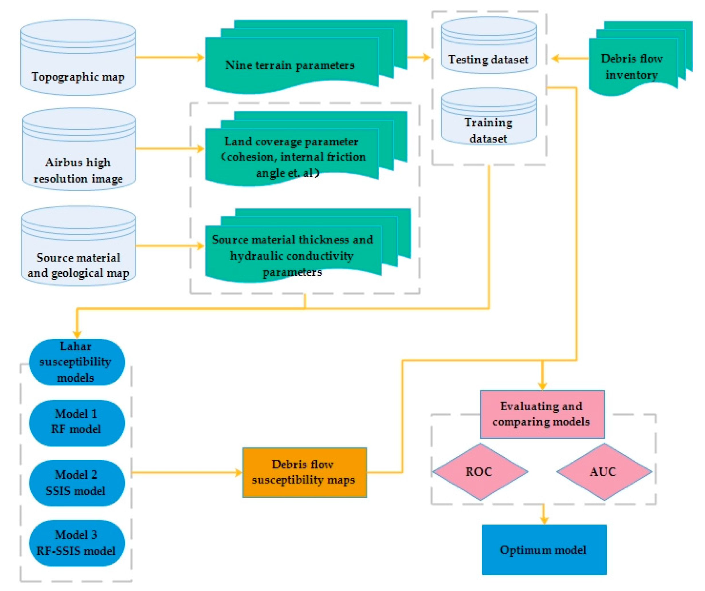
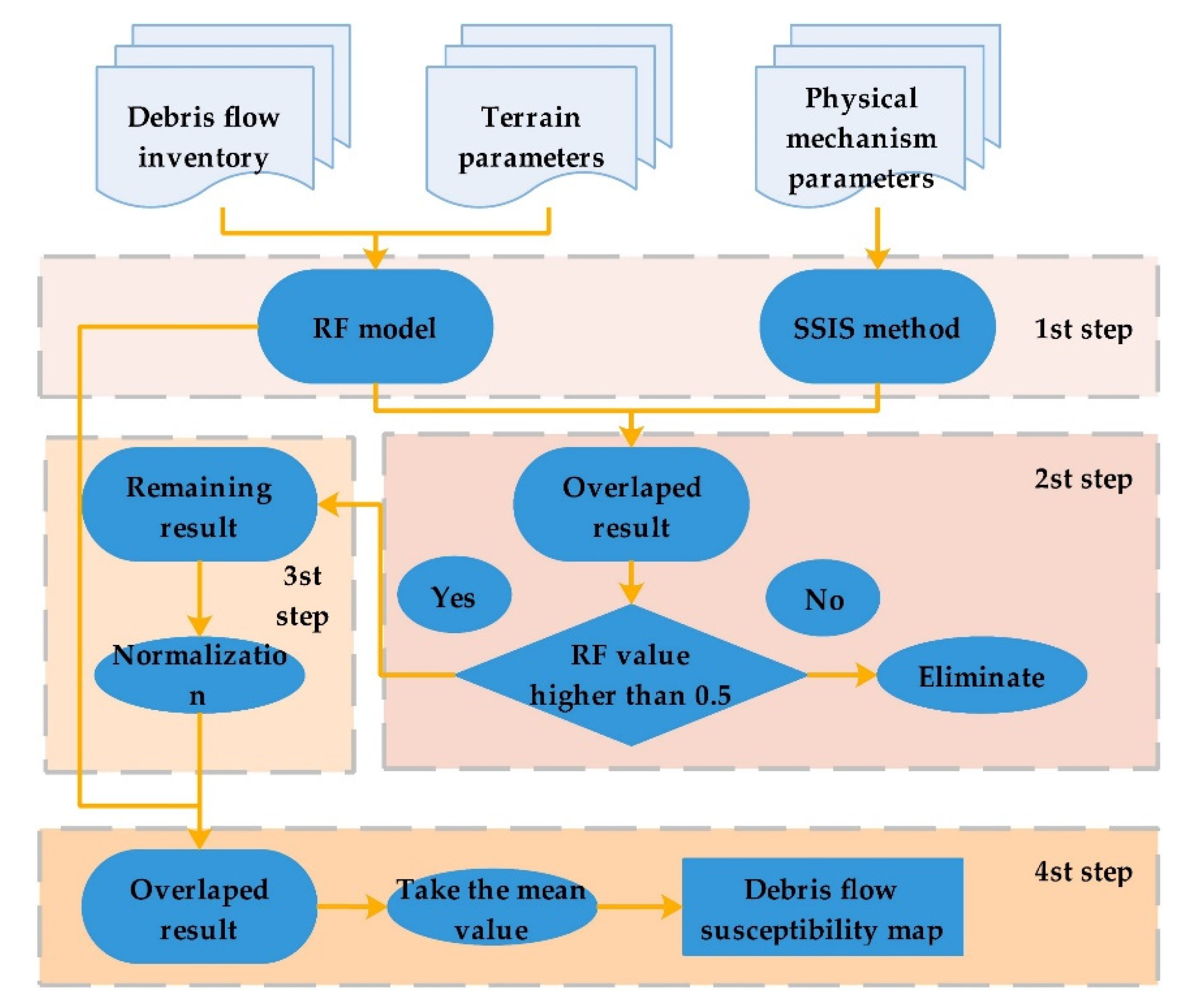
This research conducted debris flow susceptibility assessment using proposed random forest-based steady-state infinite slope method (RF-SSIS), random forest (RF) mode, steady-state infinite slope (SSIS) method, and verified the accuracy of results respectively. To find out the most optimum model. The framework of whole study is shown in
Figure 2.
First, through the topographic map, nine terrain parameters (i.e., slope, elevation, curvature, plane-curvature, profile-curvature, topographic wetness index (TWI), terrain ruggedness index (TRI), slope gradient, slope length index (SLI), and distance to rivers) were obtained, which were used in RF model. The ten physico-mechanical parameters (i.e., cohesion, internal friction angle, hydraulic conductivity, slope gradient, thickness of the loose sediments, cumulative drainage area, length of cumulative drainage, specific weight of water, specific weight of saturated loose sediments, and net rainfall) used in SSIS method were obtained from high resolution image, source material thickness (thickness of the loose sediments) map, and geological map.
Second, the terrain parameters were divided into training and testing data. The training data was used to train the RF model and calculate the susceptibility of study area. The ten physico-mechanical parameters were used to calculate the factor of safety value (susceptibility value) through SSIS method.
Third, all nineteen parameters were assigned to the RF-SSIS method to calculate the debris flow susceptibility of the study area.
Finally, the prediction accuracies of the three models were calculated and the most optimum model was obtained.
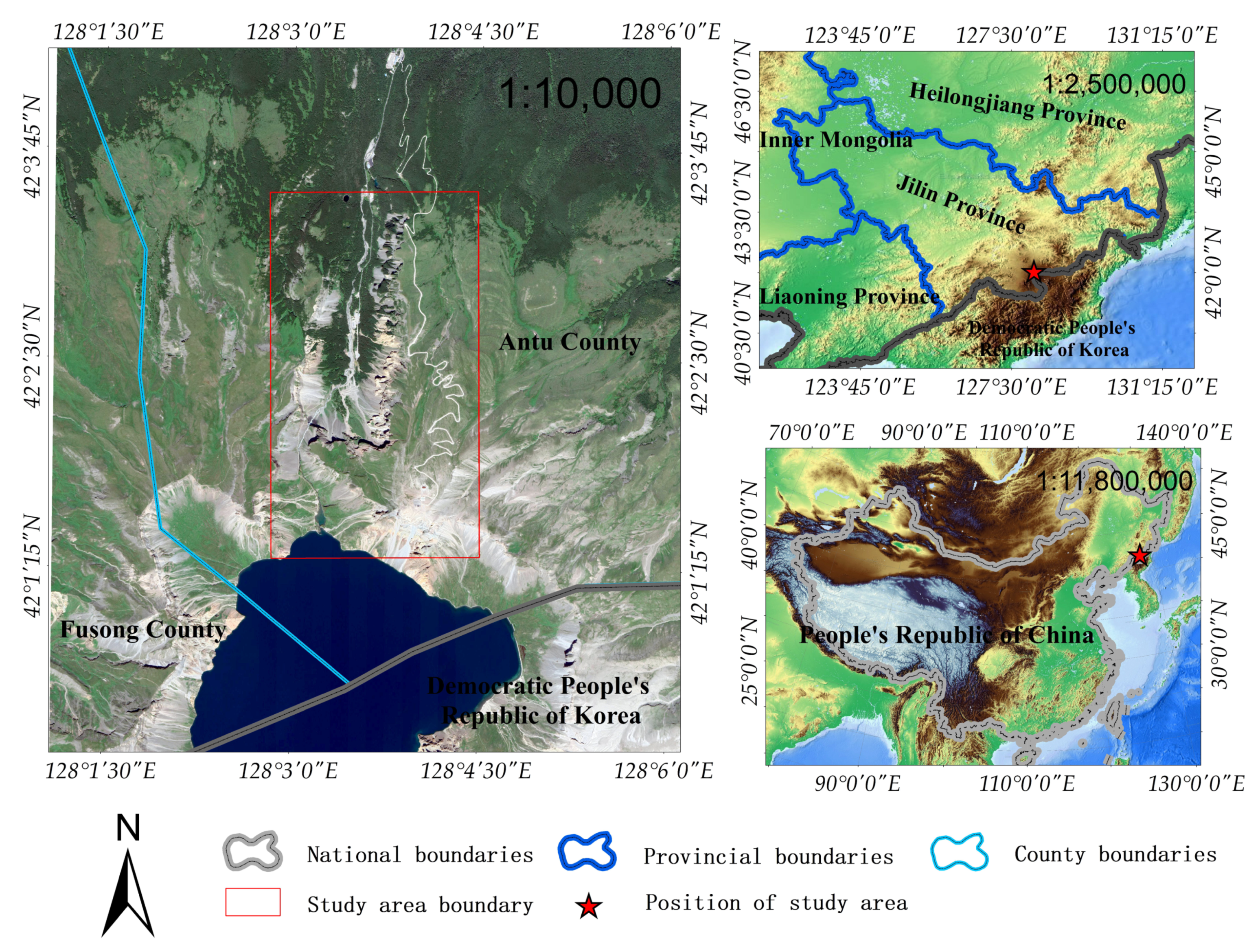
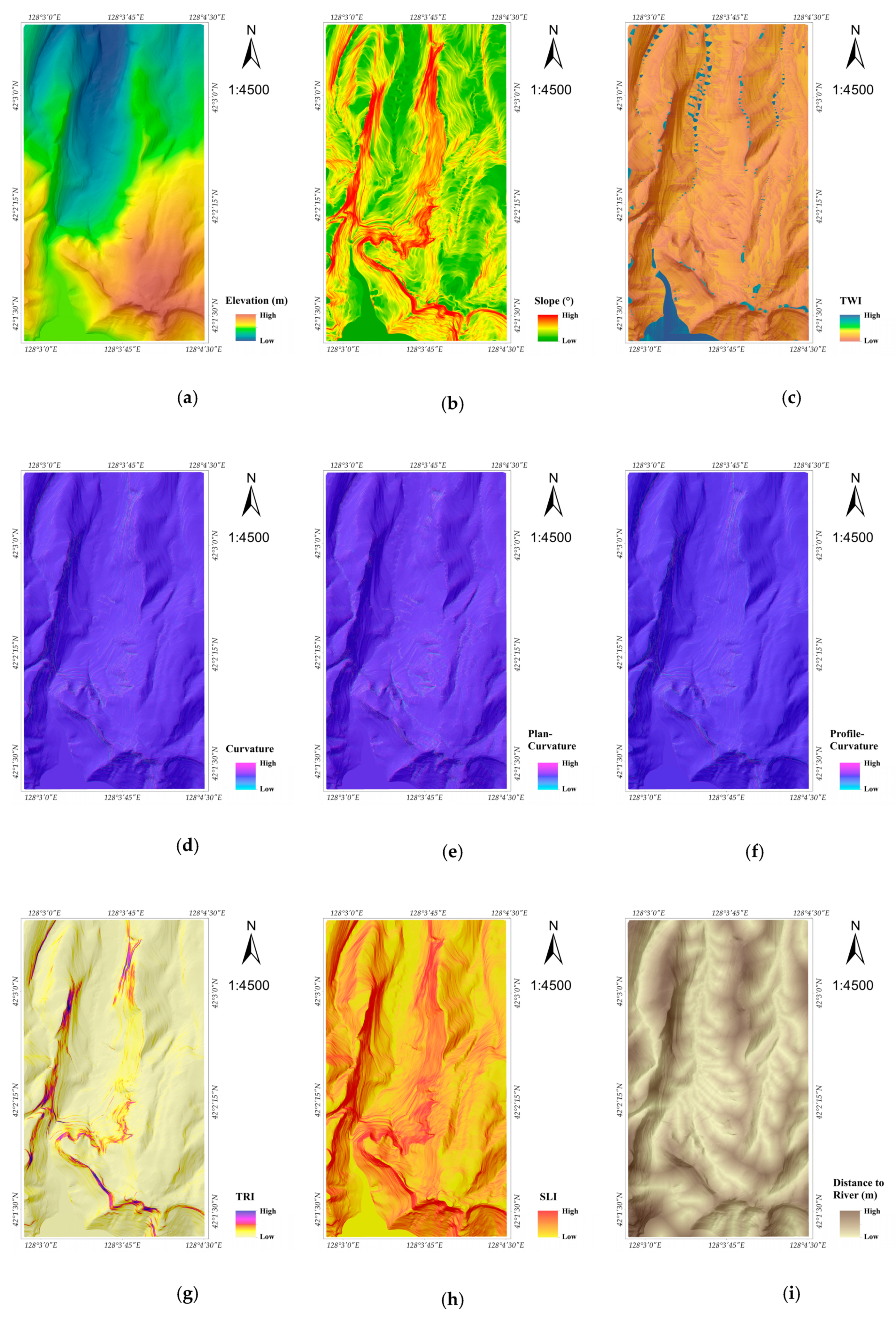
The probabilistic model was used to measure the likelihood of debris flow occurring in the terrain of the study area. Thus, only parameters that represent the complexity of the terrain were selected for computational purposes. With the help of GIS tools, the 1-m resolution digital elevation model (DEM) was obtained from a topographic map with a 1:5000 scale, as provided by the Jilin Institute of Geological Environment Monitoring (JIGEM). In the same DEM, nine parameters (
Figure 3a,b) were identified and used in the models to calculate the susceptibility of the debris flow. Such parameters include the slope, elevation, curvature, plane-curvature, profile-curvature, topographic wetness index (TWI), terrain ruggedness index (TRI), slope gradient, slope length index (SLI), and distance to rivers. For successful debris flow susceptibility assessment, it is important to focus on accuracy and a reasonably complete disaster inventory [
39]. Thus, the debris flow inventory of the study area was provided by JIGEM while recording the details, including the occurrence location, time, intensity, source area, pathways, accumulative area, and the triggering factors—time and intensity—of eight investigated debris flow events. According to Cama [
11] the debris flows can be described as rapid gravity-induced mass movements controlled by topography, which are usually triggered as a consequence of storm rainfall. Therefore, the prone area should be the source area and pathways; meanwhile, the pixels inside the accumulative area should not be included in the sample data. In this study, there are 101,830 pixels within the source area and pathways that belong to the sample data, of which 80% were selected as the training data to train the model, while the remaining 20% was used to verify the accuracy of the results.
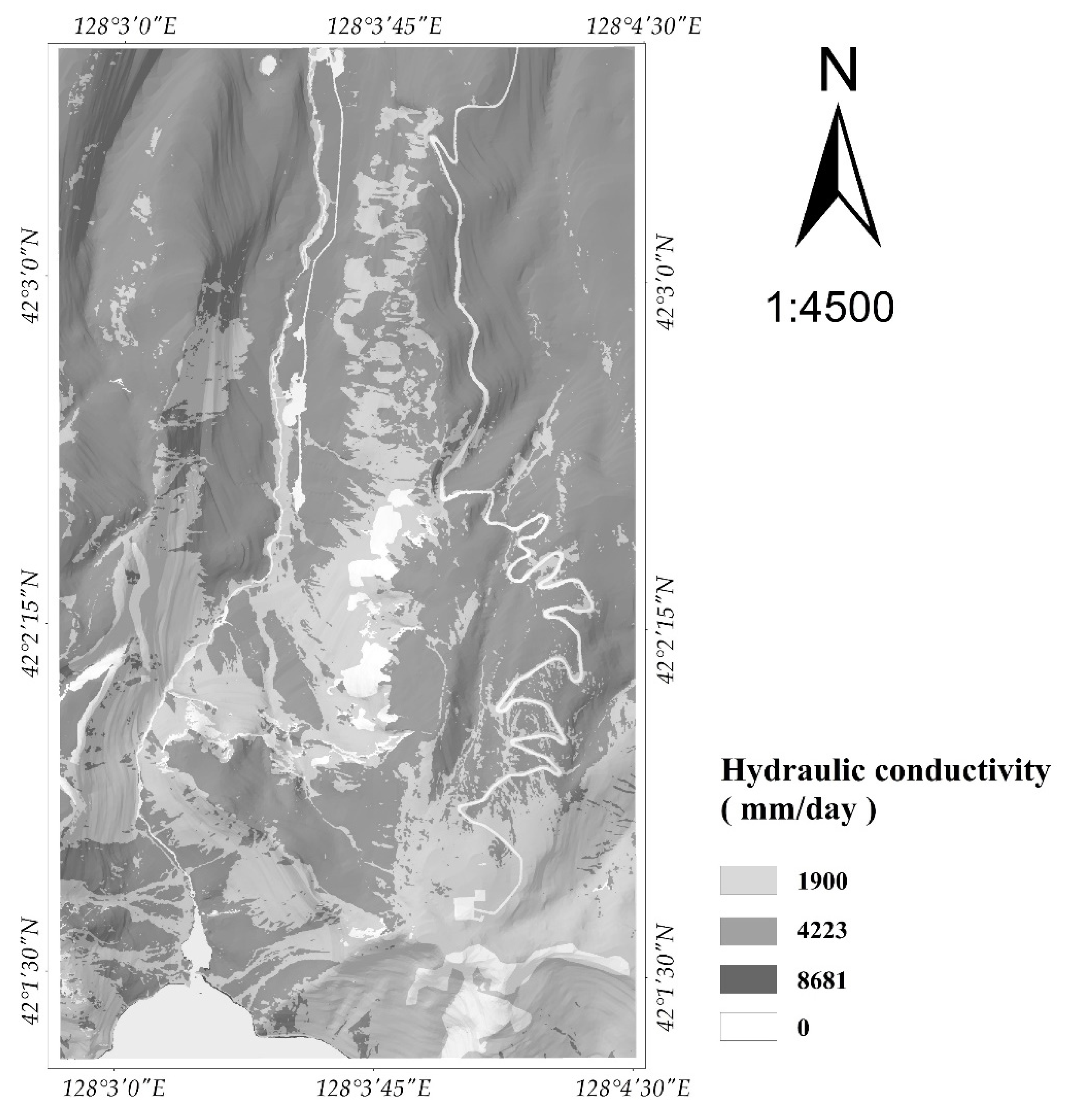
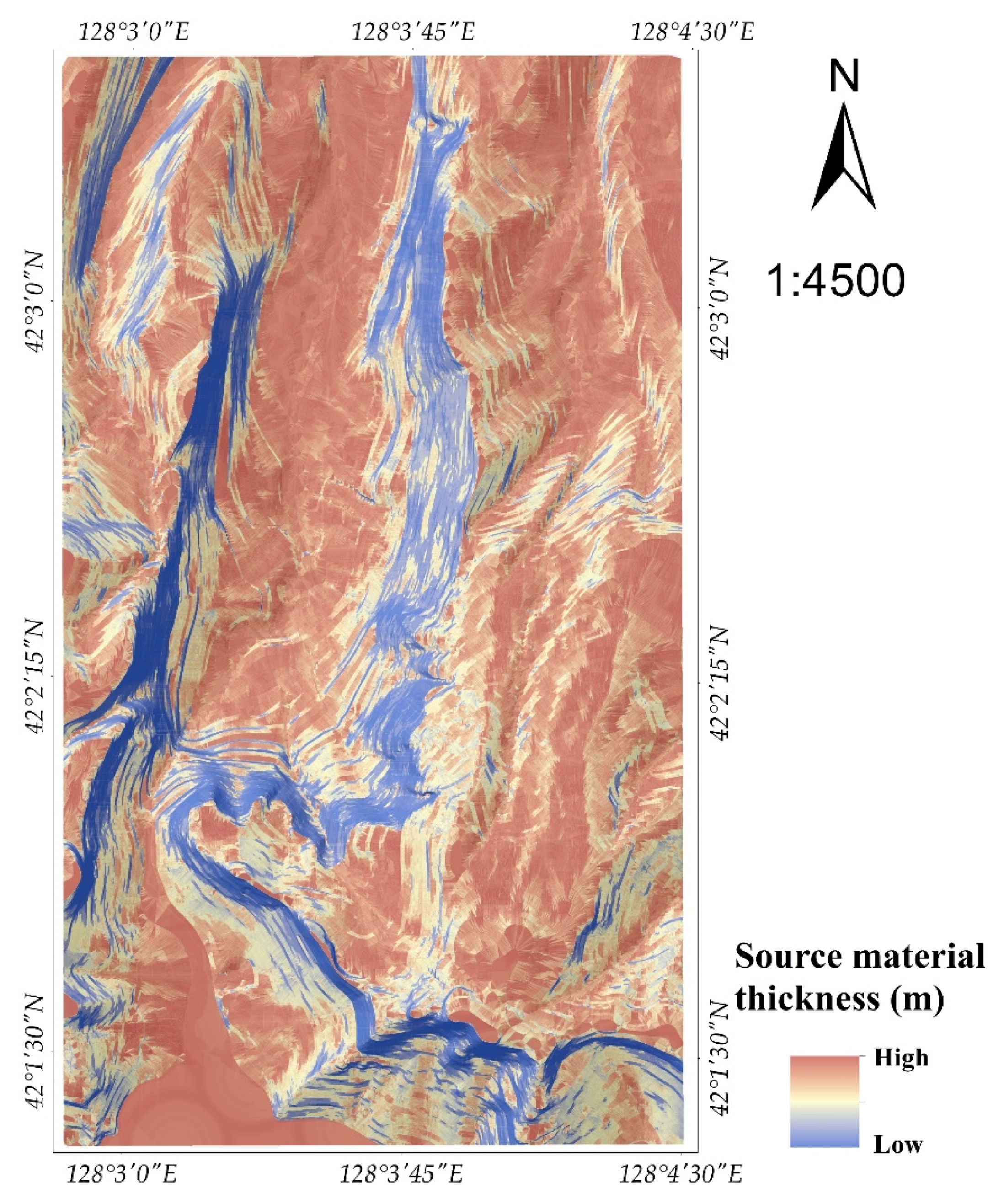
From the deterministic models used in this study, four main parameters were needed, namely, (1) internal friction angle, (2) cohesion, (3) thickness of the soil, and (4) hydraulic conductivity. Internal friction angle is the shear strength index of soil, it reveals the friction properties; cohesion is the attraction between homogeneous substance. These two parameters indicate the strength of soil stability, the higher the value means the soil is more stability. Soil is the most important component of debris flow, the thickness of soil directly affects occurrence probability and intensity of debris flow. When the thickness is equal to 0 or very small, it only can cause flood instead of debris flow. Hydraulic conductivity is the index that measures the infiltration speed and volume of water; it affects the internal balance of soil. When the internal balance breaks, the soil becomes unstable. For accuracy and an appropriate definition of the soil’s physico-mechanical properties for the given region, lab tests should be conducted. However, owing to the spatial variability of these parameters, the values of the parameters tend to vary strongly spatially, even in small areas, and thus significantly more in a medium-scale area such as the study area. Thus, on a regional scale, defining the properties of the soil through a lab test is not feasible. Therefore, some studies defined the properties of the soil based on soil maps and the support of expert criteria [
40]. They assumed that the unique physico-mechanical properties of each soil classes were homogeneous, did not vary spatially. Thus, the different physico-mechanical properties could be assigned to each soil classes with the help of experts with professional knowledge of the geological, geomorphological, and geotechnical characteristics of the study area. Notably, the correct procedure to discriminate the different physico-mechanical characteristics of the homogeneous region should be based on the soil maps; however, sometimes, the soil map was not available at the regional scale [
41]. Another way to define soil properties was to extrapolate them from geological and land coverage maps that are more ordinary. In this way, the homogeneous regions could be reclassified as a portion of the territories with the same geology formation and/or the same land coverage features. This study based on the thoughts presented by Bregoli [
40], to differentiate homogeneous soil classes based on the land coverage and geology maps (
Table 1 and
Table 2, respectively). The use of such assigned values in this study is supported by various local and international studies [
40,
42,
43,
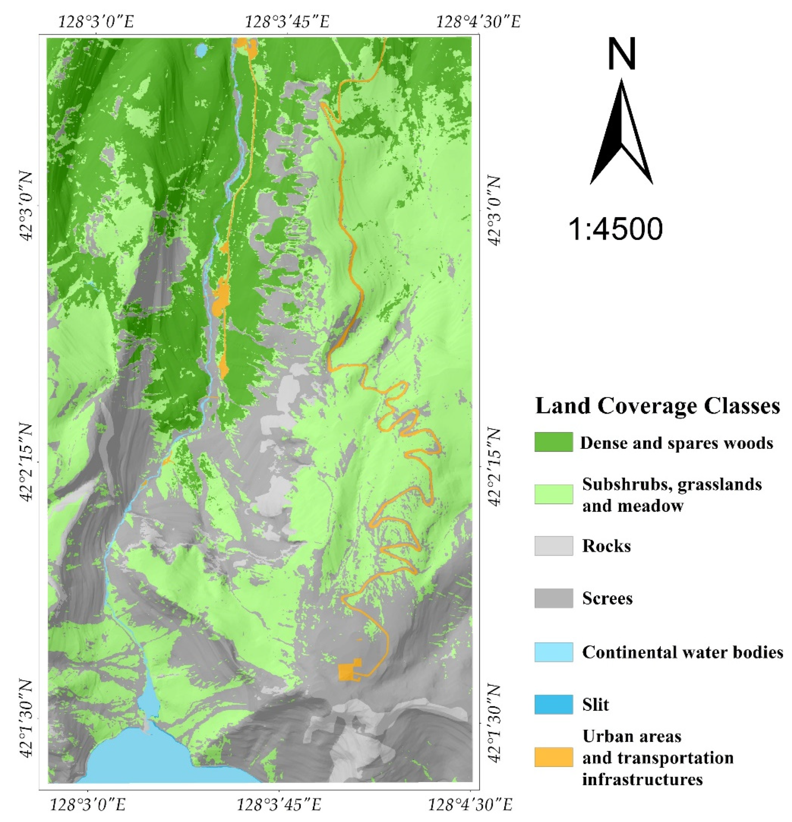
44]. In this study, the critical net rainfall threshold used was provided by the Jilin Meteorological Service, and the land coverage map was obtained from a high-resolution satellite image−Airbus with a 0.89 m spatial resolution, providing different soil classes as shown in
Figure 4. Geological and source material thickness spatial distribution maps at 1:10,000 scale was provided by the JIGEM (
Figure 5 and
Figure 6).
After the reclassification of the geology classes. Legend codes are shown in
Table 2.
After data preparation, the obtained parameter was assigned to three models to conduct debris flow susceptibility assessment. The details of three models used in this paper are shown below.
3.1. Random Forest Regression Model
As a highly flexible machine learning algorithm rising in popularity, random forest (RF) is a classifier that contains several decision trees by considering an ensemble, i.e., forest of n trees, to multiply the efficiency and predictive capability accordingly [
45]. Initially, the RF model was applied in marketing or insurance; nowadays, it is used in many probabilistic models to assess disaster susceptibility. The model has been commonly used and is well-known as an excellent means of prediction performance through a reliable processing procedure [
46,
47]. In addition, it has great tolerance for outliers and data noise and not easy to over-fit. The RF model was conducted in the following steps: (1) Bootstrap aggregation (bagging) was used to randomly extract N distinct samples from the original training sample dataset K times, and K decision trees were built based on these samples; (2) for each conditioning parameter with L attribute variables (in this case there are 9,657,550 variables in each parameter), a random constant I was assigned, and I variables were selected from L, in which I << L, because if I is higher than L, it will create a lot of null value, leading to the invalid results; (3) each node was split according to step 2 until splitting could no longer occur; (4) steps 1–3 were repeated K times to build the random forest. For classification, voting was performed to obtain the optimum result. For regression, the mean value of all trees was used, resulting in the optimum prediction result. Unselected data are referred to as out-of-bag (OOB) data, which were used to calculate the error of the model (i.e., OOB error) and are equal to the standard deviation error between the predicted and observed values. The random forest regression model was used to assess the probability of debris flow occurrence for each pixel by considering a combination of nine parameters, including curvature, TRI, and distance to the river. In the training of the RF model, the debris flow existed regions were recorded as 1, whereas the non-debris flow regions were recorded as 0. After recording, a regression was performed, and the resulting values ranged from 0 to 1. Through the different combination of these parameters, the complexity of the real terrain was explained. The area is said to have a high likelihood of debris flow occurrence if the combinations are more similar to the area where the debris flow of other similar events has already occurred. Nevertheless, in this study, the RF model was still unable to express the initiation mechanism of the debris flow disaster.
3.2. Steady-State Infinite Slope Method
As a traditional approach, SSIS method is able to estimate the factor of safety value to measure the slope stability. According to the conservation of mass and Darcy’s law, for a given cell of region with a cumulative drainage area
and length
, the steady-state condition can be expressed as
where
is the slope gradient of a given cell,
is the water table depth,
is the thickness of the loose sediments,
is the hydraulic conductivity,
is the groundwater outflow,
is the amount of rainfall, and
is the potential evapotranspiration. This leads to the value
as the net rainfall.
Another main assumption of this method is that the infiltration capacity of the soil considered far exceeds the net rainfall. Hence, over-land water can infiltrate to water instantly which can lead to the negligence of the over-land flow, in which only the groundwater flow is considered.
Combining Equations (1) and (2), the ratio between the water table depth and thickness of loose sediment/s can be derived by the following equation, as postulated by Montgomery and Dietrich [
48]:
where,
. The stability of a completely saturated loose sediment layer can be computed based on the method proposed by Skempton and DeLory [
49] and expressed as the
:
where,
is the internal friction angle
is cohesion,
and
are the specific weight of water and saturated loose sediments, respectively.
The initiation of rainfall-triggered debris flow was due to the high-pore-pressure reducing ratio between the resisting and acting stresses. The condition is that, when the ratio is lower than 1, the loose sediment layer becomes unstable, initiating the debris flow disaster. The behavior is described by the common Mohr-Coulomb failure approach to the infinite slope stability [
50]. But, when the soil thickness was greater than the length and width of source materials, this assumption no longer holds up. Despite the thickness of pyroclastic debris in this study ranging from 0 to 10 m, it was still far from its length and width. In this case, the steady-state infinite slope (SSIS) method was adopted to measure the
FS of the study area. The SSIS method measures the slope stability through a simplified way to calculate the water pore pressure [
51,
52]. At first, the method assumed the study area to have rainfall of constant intensity with an indefinite duration, causing the water table to reach steady-state conditions. The slope meets the limit equilibrium condition when
equals to 1, and if
, the slope is recognized as unstable.
There are two limit cases that complicates the assessment based on Equation (4). These are the unconditionally unstable case (UUC) and unconditionally stable case (USC), respectively. While UUC represents the unstable slope found in a dry condition, such as a steep slope, USC represents the stable slope found in a completely saturated condition, such as that of a flat area. The two cases are indicated based on Equations (5) and (6). In this study, any region falling under these two conditions was not considered, and hence, removed from the general calculation. Generally, regions with a slope higher than 45° were eliminated along with flat regions.
The SSIS method used ten parameters including cohesion, internal friction angle, and water conductivity to calculate the value of the slope. The value can also indicate the susceptibility of debris flow. In this analysis, a higher means that the pixel was more prone to debris flow occurrence.
3.3. Random Forest Model-Based Steady-State Infinite Slope Method
Despite the good performance exhibited by the RF model and SSIS method in debris flow susceptibility assessment, the two are not without some significant limitations, hindering the suitability of assessment performance. During susceptibility assessment, the RF model considers an abundance of background information i.e., topographical information for calculations, making it somewhat sensitive to terrain prone to debris flow occurrence. However, it did not consider the initiation mechanism of debris flow during calculation; thus, physico-mechanical parameters were not considered in the calculation. On other hand, the SSIS method was used to measure the slope stability by considering the parameters such as cohesion, internal friction angle, source material et al., which is closer to the real debris flow initiation mechanism. However, owing to the spatial variability of physico-mechanical parameters, it is hard to obtain the values of these parameters. But, because the cumulated drainage area and the slope factors were obtained from the high-precision DEM, so only these data were precisely enough for indicating the influence of real terrain conditions on debris flow. In this study, the remaining physico-mechanical parameters were assigned based on the land coverage and geological map. Thus, the precision of remaining parameters was not enough to indicate the influence of real terrain conditions on debris flow, making incomplete and inappropriate results with respect to the actual situation. It is because of such drawbacks that the study uses a random forest model-based steady-state infinite slope method (RF-SSIS) to calculate the debris flow susceptibility, producing an entire new way of thinking, as shown in
Figure 7.
First, the RF model (model 1) and SSIS (model 2) method are used to successfully conduct the susceptibility assessment in the study area, in addition, neglecting the use of Equations (5) and (6) to eliminate the unqualified area of model 2.
Second, the results from Model 1 and Model 2 were overlapped, and two results (FS value and RF results) were assigned to each pixel.
In this case, a threshold of 0.5 was set, and filtering was performed to retain the pixels with RF values greater than or equal to 0.5. This allowed to eliminate pixels with no-suitable terrain condition.
Third, only the FS value was retained and the RF result value was deleted. In this case, only the region with the terrain condition suitable for debris flow occurrence has the FS value, and the FS value of other regions was 0. After that, centered as 1 and normalization was performed of the FS result obtained from step 2. Normalization matches the quantized range of FS with the RF result. Furthermore, the slope reached a critical condition at FS = 1.
Finally, results obtained from step 3 were overlapped with the RF results obtained from step 1. In this way, each pixel had two values again. Then, the mean of these two values was taken, and a result was obtained with values ranging from 1 to 0. The closer this value is to 1, the more this pixel represent an area prone to debris flow.
This method through Step 2 was used to remove the regions where the terrain conditions were not suitable for debris flow occurrence. This is because the RF model was considered for the abundant background information (i.e., terrain information); thus, its result can reveal the influence of the actual terrain on the debris flow more objectively. After elimination, the terrain conditions of the remaining regions (RF > 0.5) were considered debris-flow-prone areas. The final mean value indicates both the influence of physico-mechanical properties and the terrain conditions of the occurring debris flow.
3.4. Receiver Operating Characteristic Curve
The performance of the prediction accuracy for debris flow susceptibility can be assessed using the receiver operating characteristic (ROC) curve method, which plots the true positives rate (i.e., sensitivity) versus the false positives rate (i.e., 1-specificity), which was used to measure the goodness-of-fit of the model prediction. The true positives rate is the ration between number of true positives pixels (TP) and number of positives pixels (P). The false positives rate is the ration between number of false positives pixels (FP) and number of negative pixels (N). TP means the pixels classified as debris-flow prone by model, and belongs to the pixels where the debris-flow actually occurred before classification as well. FP means the pixels classified as debris-flow prone by model, but belongs to the pixels where the debris-flow does not occur before classification. P means all the pixels inside the actually occurred debris-flow. N means all the pixels outside the actually occurred debris-flow. P is the sum of TP and FN (false negative). N is the sum of FP and TN (true negative). FN means the pixels classified as debris-flow non-prone by model, but belongs to the pixels where the debris-flow actually occurred before classification. TN means the pixels classified as debris-flow non-prone by model, and belongs to the pixels where the debris-flow does not occur before classification as well. The area under the curve (AUC) value represents the area under the ROC curve, which is utilized to quantitatively show the results of the ROC. The AUC varies from 0.5 (diagonal line) to 1, with higher values indicating better predictive capability of the model.
4. Results
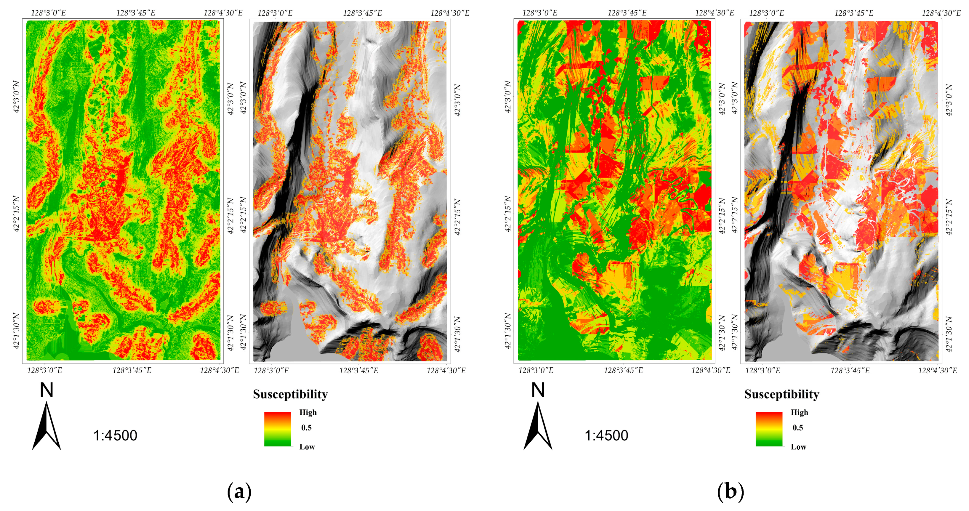
Susceptibility assessment results of the RF model and SSIS method are shown in
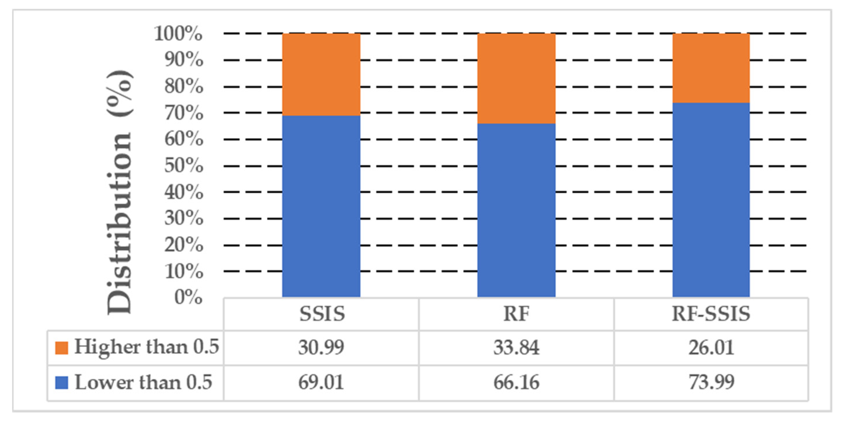
Figure 8a,b, respectively. The regions of the RF results with values greater than 0.5 account for 33.84% of the entire study area (
Figure 8a), mainly distributed around the major gullies. The regions with
FS values (SSIS results) greater than 1 account for 30.99% of the entire surveyed area (
Figure 8b), mainly distributed in the regions with slope ranging from 5° to 40°. When assessing the OOB error, after establishing 100 trees, the error rate of the RF model reached a minimum with the tendency of becoming stable. Thus, this study used an RF model with 300 trees and conducted a debris flow susceptibility assessment; as such the results are comparatively credible.
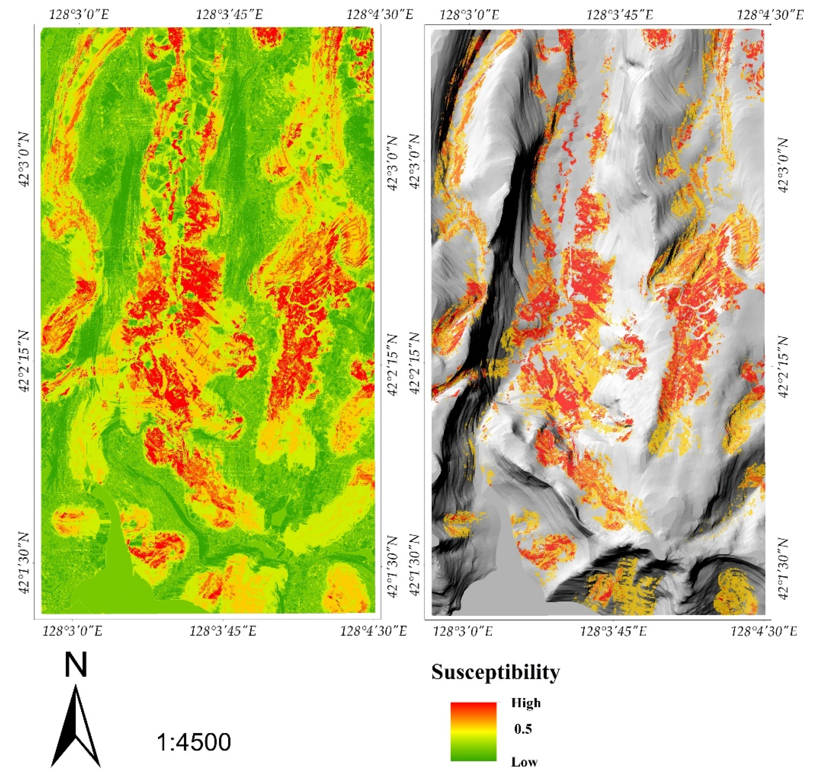
The result of the RF-SSIS is shown in
Figure 9; in this result, the debris-flow-prone region, i.e., the region with pixel values higher than 0.5, accounted for 26.01% of the entire study area (
Figure 10). The elimination of the region was conducted based on the result of Model 1 (RF model); thus, the distribution of the debris-flow-prone area of the RF-SSIS was generally similar, even though the area decreased by 7.83% (
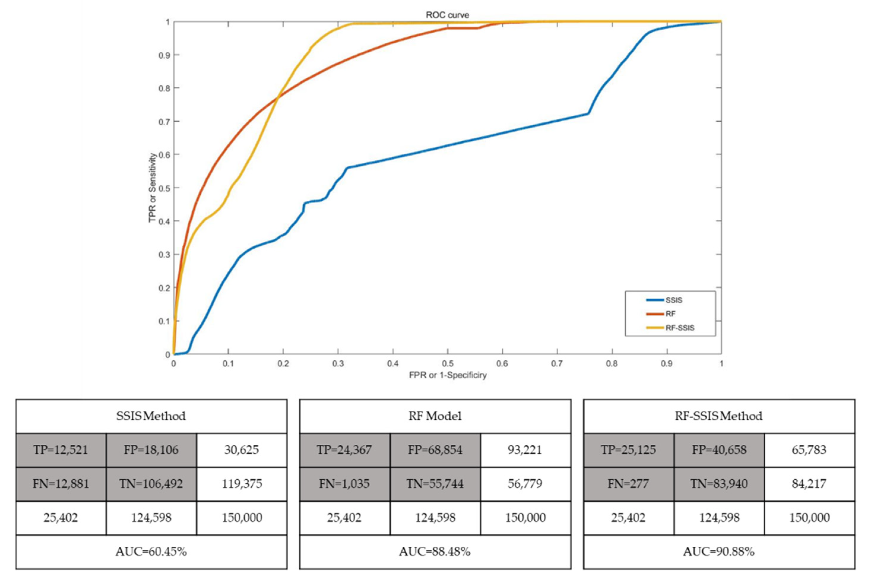
Figure 10). After the debris flow susceptibility assessment was conducted, the remaining 20% of the sample data was used to verify the accuracy of the result. It shows that the prediction accuracy (AUC) of Model 1 (RF model) was 88.48%, and that of Model 2 (SSIS method) was 60.45% (
Figure 11). Thus, we noticed that the gap in the prediction accuracy of these two models was significant. Furthermore, the prediction accuracy (AUC) of the RF-SSIS method reached 90.88%, with the AUC value improving by 2.4% and 30.43% (
Figure 11), compared with the RF model and SSIS method, respectively. For the RF model, the proposed RF-SSIS method not only improved the prediction accuracy but also reduced the area of the debris-flow-prone region. This is due to the fact that the method identifies and eliminates some regions that are unsuitable for the occurrence of debris flow in terms of the mechanism or physico-mechanical properties. Then, as opposed to the SSIS method, the RF-SSIS method determined the favorable terrain for the occurrence of debris flow based on the abundant background information, with better performance than that provided by the elimination of the unfitted area based on Equations (5) and (6). Afterwards, the susceptibility assessment through the aspect of mechanism and terrain conditions and the result was more reliable and accurate.
5. Discussion
On the basis of multi-source data, RS, and the GIS technique, the debris flow susceptibility assessment of the study area was implemented using three different models (RF, SSIS, RF-SSIS). The RF model and SSIS method used in this research represented the heuristic/probabilistic and deterministic models, respectively. The SSIS method (i.e., deterministic model) predicted the future according the current situation [
53,
54,
55] and the RF model (i.e., heuristic/probabilistic model) predicted the future based on the past and present [
56,
57,
58,
59,
60]. Each of these methods has a robust theoretical basis and practical support; however, each has outstanding advantages and also some irreparable disadvantages. The SSIS method, couples a Mohr-Coulomb failure mechanism with a steady state lateral flow to calculate susceptibility. When using SSIS method at a regional scale for assessment, the disadvantages of this method still caused a lower prediction performance. Meanwhile, the SSIS method assumed that each of the pixels inside the study area was an independent infinite slope. So, the pixel interconnection was neglected. [
40,
61]. However, in actuality, the terrain condition of the source area and pathway of debris flow was extremely complex, meanwhile, every pixels were interacted with the neighboring eight pixels, also affected by them; for instance, it was assumed that before the occurrence of debris flow, each of the pixels inside the region had a slope gradient that differed from others. Owing to the fact that the slope of some pixels may approach 0° or be higher than 45°, these pixels were considered as non-prone by SSIS method. But owing to these pixels inside the source area or pathway region, they actually belong to debris-flow prone in reality. In addition,
Figure 8b shows that many plain slope regions were recognized as debris-flow-prone areas. As for every single pixel inside these regions, the parameters of each pixels supported them to classified as debris-flow prone; however, from the regional perspective, the terrain condition of these regions cannot support this classification. For the RF model, owing to the accessibility of high-precision data, it can fix the disadvantage of SSIS method in obtaining accurate and reliable physico-mechanical parameters. The parameters like LSI, TWI, and TRI can reflect the interconnection of pixels. Thus, one of the great advantages is that this model can effectively determine the regions with the terrain condition suitable for the occurrence of debris flow under the support of sufficient disaster inventory and geo-information data. But this is also its biggest weakness, because the RF model was limited to just locating the appropriate regions; yet, there was a lack of consideration of starting mechanism or physico-mechanical properties, causing some regions with suitable terrains to be considered as debris-flow-prone regions, but because of the restrictions on the physico-mechanical properties such as hydraulic conductivity or thickness of the loose sediment, these regions are hard to become debris-flow-prone regions in reality. Even if one tries to assign physico-mechanical properties parameters to the RF model, the lack of the actual values before debris flow made it impossible to achieve.
The main thought of the RF-SSIS method proposed by this research was to integrate the strong points of SSIS and RF models to improve the prediction accuracy of the debris flow susceptibility assessment from entirely different perspectives. The strong point of the RF model was to seek terrain prone to debris flow [
47], with the result value ranging from 0 to 1 and 0.5 as the critical point. Regions with values higher than 0.5 were classified as debris-flow-prone regions, whereas the closer this value is to 1 signifies regions more prone to debris flow. Therefore, filtering was conducted, eliminating the non-conforming regions in the SSIS result based on the condition that the pixel RF value was equal or greater than 0.5. After the elimination, the terrain conditions of the remaining regions was considered as prone to debris flow. Meanwhile, the
FS value of the pixel further quantified the likelihood of debris flow occurrence (i.e., the susceptibility) from the aspect of physico-mechanical properties and initiation mechanism [
62]. Even if the eliminated regions had a higher
FS value but the basic terrain conditions were unsuitable, these regions still did not belong to the debris-flow-prone area. After the remaining SSIS result was overlapped with the result of RF model, the mean value of these two were taken, the RF-SSIS models result was obtained with value ranging from 0 to 1. The RF-SSIS models not only evaluated the debris flow susceptibility from the perspective of the deterministic model but also evaluated the debris flow susceptibility from the perspective of the heuristic/probabilistic model. In addition, when the RF-SSIS result was higher than 0.5, it must have meant that these pixels were prone to debris flow, and there were several situations that lead to the values greater than 0.5. First, these pixels were suitable for the occurrence of debris flow both from the terrain condition and the physico-mechanical properties (both the values RF and SF were higher than 0.5); thus, the final susceptibility values were higher than 0.5. Second, in the case in which one condition was very suitable for debris flow, e.g., the very suitable region terrain conditions (RF value higher than 0.7) with unsuitable physico-mechanical properties (SF value between 0.3 to 0.4), synthetical considerations determined this region as debris-flow-prone regions (final value higher than 0.5). If both conditions were not suitable (both lower than 0.5) or one condition was extremely unsuitable (equal to 0), this region must not be the debris-flow-prone area because the final value was lower than 0.5.
As shown in
Figure 11, when comparing the proposed method with the RF model, the determination of true-positive pixels was improved slightly, but the determination of false-positive pixels was improved significantly. From
Figure 8 and
Figure 9 we can notice the pattern mentioned before, the reduction of the prone area outside the debris-flow-existed region was significant; however, the status inside the debris-flow-existed region was basically unchanged. This is due to the proposed RF-SSIS method inheriting the excellent diagnostic performance of the RF model (i.e., heuristic/probabilistic model) for the region where a debris flow disaster already existed [
63]; meanwhile, this method further refined the debris-flow-prone area from the suitable area terrain condition based on the physico-mechanical properties. This is the reason why the proposed RF-SSIS method had better predicting performance than the RF model; however, the prediction accuracy did not improve very well, because under the support of historical data, the RF model exhibited very high prediction accuracy for debris-flow exist areas [
14]; so the space for improvement was limited and difficult to further refine. Therefore, even though the determination of FP was improved significantly, the RF-SSIS method classified just 758 more TP pixels than did the RF model; the determination on TP was less improved, causing an insignificant improvement in the prediction accuracy. However, as the most representative model of heuristic/probabilistic model, the RF model showed excellent performance in previous debris flow susceptibility assessment [
64,
65], despite the prediction accuracy of the proposed RF-SSIS method improved slightly compared to the RF model; nevertheless, the assessment method was still shown to have been improved. For the SSIS method, an assessment was conducted based on the triggering mechanism and physico-mechanical properties, and when this method was used in regional assessment, it also demonstrated good performance [
66,
67]. Through
Figure 11 the prediction accuracy of proposed RF-SSIS method is shown to improve significantly as that of the SSIS method, as the SSIS method was a prediction method that calculates the susceptibility based on the current data. Thus, the prediction performance on existing debris flow regions was relatively lower. However, the final result of the RF-SSIS method not only indicated the influence of the terrain on the debris flow but also the influence of the physico-mechanical properties on the debris flow; thus, the prediction accuracy for the region where the debris flow disaster already exist was significantly higher than that for the SSIS model. Meanwhile, this method inherited the performance of SSIS models in determining the area where debris flow would not occur; thus, the false-positive pixel determination was improved significantly compared to that of the RF model. Thus, these situations resulted in an improvement in the prediction accuracy performance.

 ,
, 


