Flood Hydraulic Analyses: A Case Study of Amik Plain, Turkey
by
 , and
, and
Fatih Üneş
1, 
Yunus Ziya Kaya
2,
Hakan Varçin
1,
Mustafa Demirci
1,
Bestami Taşar
1 and
Martina Zelenakova
3,* 1
Department of Civil Engineering, Faculty of Engineering and Natural Sciences, Iskenderun Technical University, Iskenderun 31200, Hatay, Turkey
2
Civil Engineering Department, Faculty of Engineering, Osmaniye Korkut Ata University, Osmaniye 80100, Turkey
3
Institute of Environmental Engineering, Faculty of Civil Engineering, Technical, University of Košice, Vysokoškolská 4, 040 01 Košice, Slovakia
*
Author to whom correspondence should be addressed.
Water 2020, 12(7), 2070; https://0-doi-org.brum.beds.ac.uk/10.3390/w12072070
Submission received: 21 June 2020
/
Revised: 14 July 2020
/
Accepted: 16 July 2020
/
Published: 21 July 2020
(This article belongs to the Special Issue Urban Rainwater and Flood Management)
Abstract
:In recent years, significant flood events have occurred in various parts of the world. The most important reasons for these events are global warming and consequent imbalances in climate and rainfall regimes. Many studies are performed to prevent the loss of life and property caused by floods. Many methods have been developed to predict future floods and possible affected areas. Developing computer and numerical calculation methods gives opportunities to make simulations of flood hazards. One of the affected areas, which is also one of the world’s first residential districts at Hatay in Turkey, is the Amik Plain. In this study, the floods on the Amik Plain in Hatay province are analyzed. Hatay airport was also affected during floods since 2012 and serious material damage occurred. For this purpose, Google Earth Pro software was used to obtain maps of the basin where the airport is located and the rivers it contains. Afterwards, Hydrologic Engineering Center’s River Analysis System module (HEC-RAS) was used for the hydraulic and hydrological definitions of the river basin. The results of numerical models are presented as simulated maps.
1. Introduction
Flooding is a condition that causes water and soil environments to be disturbed in areas that are not normally submerged owing to increased flow and rising level in a stream. This situation may harm humans and animals and damage land and property near the river. In Turkey, 695 floods occurred from 1975 through 2010, causing great economic losses second only to earthquakes. A total of 634 people lost their lives in these floods, 810,000 hectares of land were left under water, and the total loss was 3.717 billion dollars. During this period, the distribution of flood losses by sectors was found to be 45% agricultural areas, 32% settlements and infrastructure, 7% portable goods and vehicles, 1% transportation, and 15% in other areas [1,2]. These stats show that flood is an extremely serious and important issue. In addition to saving many lives, the works to be done to predict floods and protect them from danger will contribute a lot to the national economy. The main purpose of this study is to investigate how vulnerable the Amik plain is against flood disasters using geographic information systems and HEC-RAS.
Flood precautions and recreation studies are performed by state hydraulic works (DSI) in Turkey. State hydraulic works (DSI) is an institution responsible for the planning, management, development, and operation of all water resources in the country. It is the responsibility of this institution to establish the flow rate values of the floods formed and the establishment of flow monitoring stations on the streams for the purpose of labor and to prepare reports of floods.
Monitoring of floods occurring in the Amik plain started with four current observation stations established in 1956. These stations are located on Asi, Afrin, Karasu, and Büyük Asi in Antakya after the combination of these three branches. The first flood, after receiving current observations, occurred in 1956. In this first flood, the flow rate of Afrin was 464.0 m3/s, Karasu was 123.0 m3/s, and Asi was 274.0 m3/s. In the second flood event, which was occurred in March of 1969, the flow rate of Afrin channel was 710.0 m3/s, Karasu was 268.0 m3/s, and Asi was 167.0 m3/s. In the flood, 15,780.0 ha area was submerged. In April 1975, Asi River was at full capacity with 180.0 m3/s and the extra flow rate was discharged to Amik Plain as 50.0 m3/s. Approximately 1500.0 ha of cultivated land was submerged. Similar floods occurred in 1976, 1980, 1987, and 1998 and affected many agricultural lands. In Antakya flood, which occurred on 8–9May 2001, in the center of Antakya and Amik Plain, a total of 569.0 kg of precipitation fell in 48 h, with 137.0 kg in the first 24 h and 432.0 kg in the second 24 h. Considering that Hatay’s average rainfall for many years is 856.0 kg, the ratio of precipitation falling in 48 h to annual precipitation is 67%. This flood caused loss of life and property and the region was declared as a disaster area. In the floods that occurred in the Amik Plain in 2002 and 2003, large agricultural lands were flooded, and caused material damages. In this study, the flood that occurred in the Amik Plain between 27 January and 14 March 2012 is investigated. In the mentioned flood, an area of 13,000 hectares was affected and a total of 8465 ha of agricultural land, roads, bridges, settlements, and Hatay Airport was exposed to flood waters [3]. The floods listed above are repeated frequently and reach dangerous levels for the region. For this reason, it is extremely important to determine the size of the floods that may occur and the areas they affect.
After the floods that occurred, DSI obtained the flow values from the flow monitoring stations on the rivers and made them into reports. For the examination of these reports, their discharge capacities were increased by enlarging the cross-sections of the streams for the protection from floods. Embankments have been made for the purpose of flood protection along the rivers. However, these precautions did not provide a definitive solution. Estimating the size of the floods that may occur and the areas they affect will make important contributions to the work to be done. However, this is a very difficult problem owing to the number of unpredictable parameters.
Numerous methods have been developed recently to make calculations or estimations about the definition of flood areas. Zeleňáková et al. worked on a risk-based approach to flood modelling of Slatvinec stream [4]. Serencam studied the negative effects of possible floods in a specific part of Trabzon, Turkey [5]. Kowalczuk et al. used HEC-RAS software to simulate river flow [6]. Abd-Elhamid et al. researched flood prediction and mitigation for coastal tourism areas as a case study in Hurghada, Egypt [7]. Romali used a GIS-based approach for flood plain mapping in Segamat Town, Malaysia [8]. Ben Khalfallah et al. also used GIS tools and HEC-RAS software together to prepare a spatiotemporal flood plain map as a case study of the Majerda River, Tunisia [9]. In another GIS-based research project, Curebal et al. generated a model for flash floods in Keçidere, Turkey [10]. Oana-Elena et al. evaluated flood event susceptibility analyses on cultural heritage in Sucetiva, Romania [11], and Romanescu et al. prepared a case study of flood vulnerability assessment for Marginea village in Romania [12].
Natural disasters are defined as inevitable, irrepressible, irresistible events, but when anticipated, the amount of damage that may be generated can be reduced when suitable measures are taken. With this in mind, depending on the accuracy of the data used in the study, pre-modeling and simulating floods, demonstrating acceptable results modulated with structural or non-structural prevention measures, will minimize the losses [13,14,15,16]. Data such as discharge, land cross section, Manning coefficient, and topography scale are used for flood modeling in the present study. Various computer programs can be used for this purpose. One of them is the HEC-RAS program, which can be modeled for one-dimensional steady or unsteady flow.
Study Area
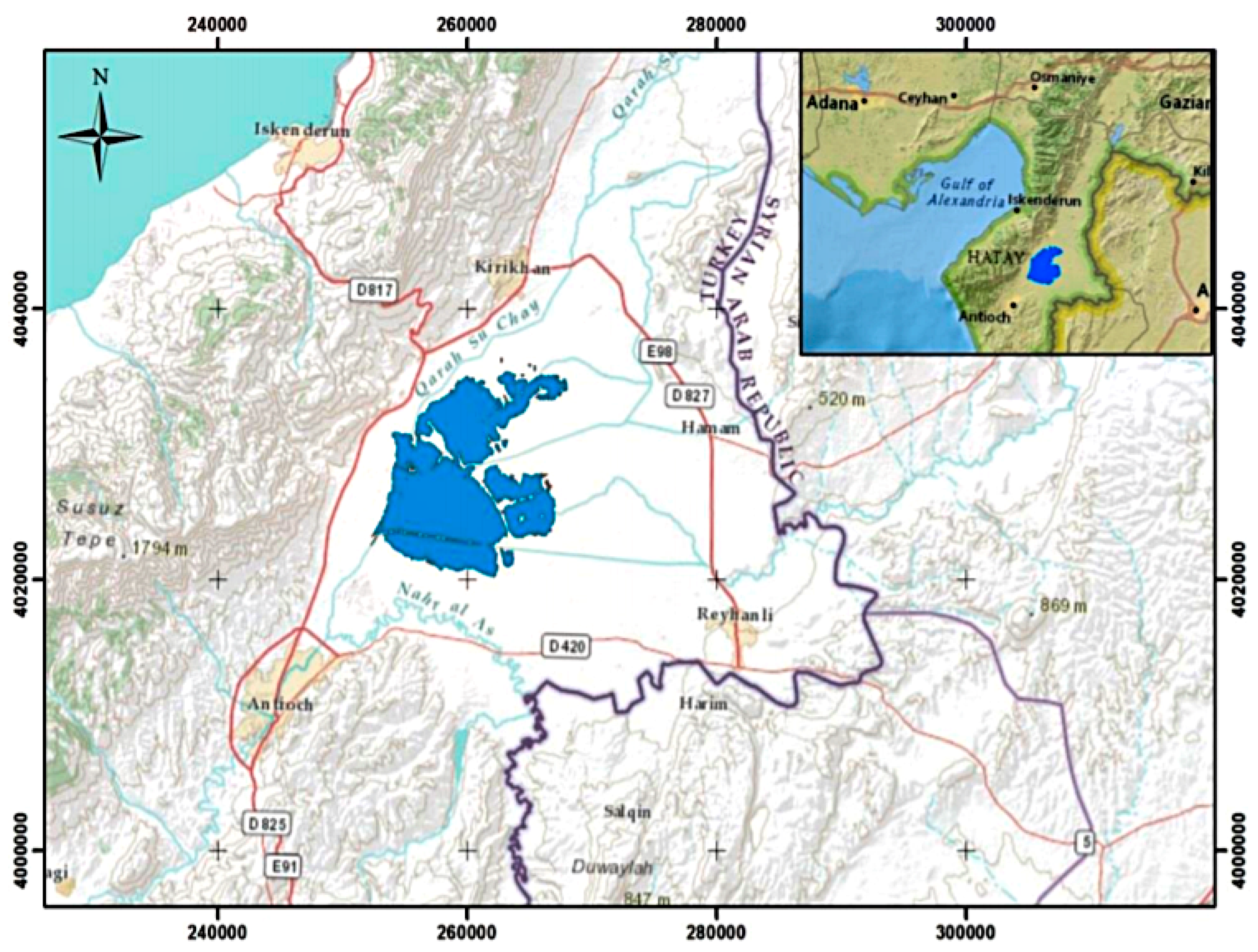
The Amik Plain in Hatay Province lies in south-east Turkey with the Kırıkhan district to the north, the Reyhanlı district to the south, the Syrian border to the east, and the Kırıkhan–Antakya road to the west.
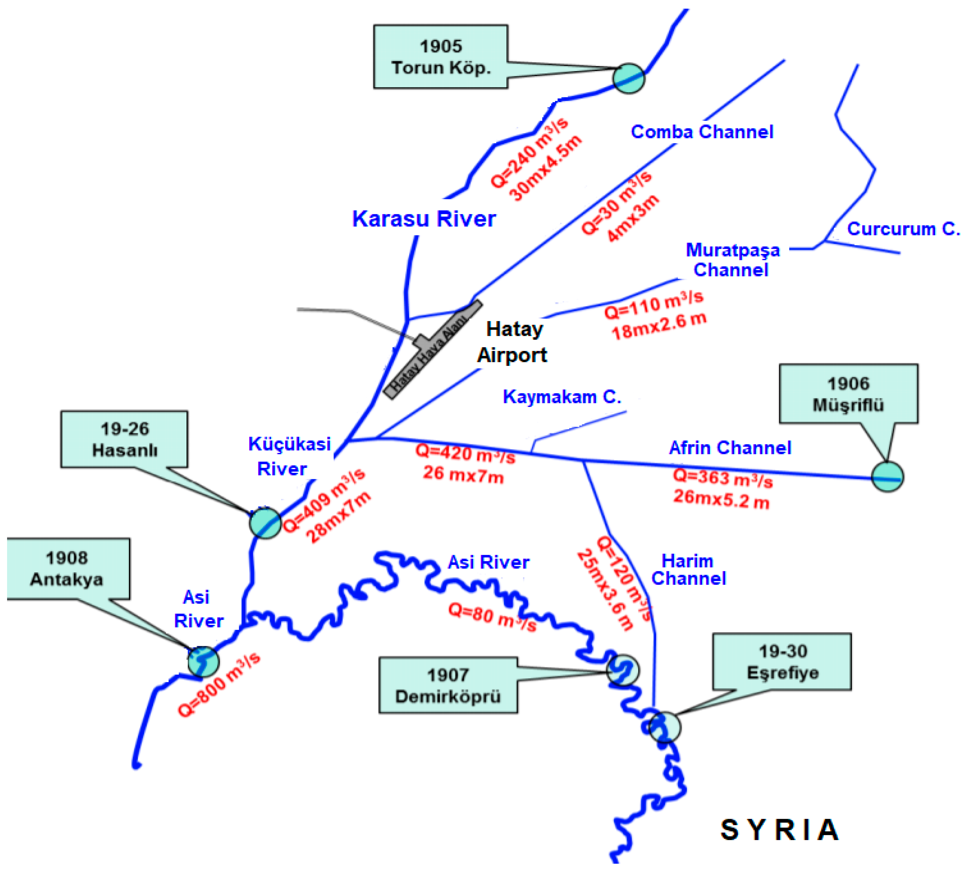
The Plain also includes a small piece of land on the left bank of the Asi River, on the Antakya-Reyhanlı road, extending to the south. The width of the Plain is approximately 36 km, the length is 40 km, and the elevation is between 80 m and 250 m [1]. The Amik Plain’s name comes from the natural Amik Lake, which is shown in Figure 1. As the flood area and lake level in the old lake were very variable, in 1940, it was designated for drying and flood protection and Amik Lake reclamation works. The Amik Lake Drying Technical and Economic Feasibility Report—Amik Lake Project was prepared in 1966 by IECO (International Engineering Company). The Karasu River, Afrin River, and Muratpaşa flood canals were discharged through the lake bed to enable the canals to connect with the Small Asi River, and the lake was dried in 1972. The flow observation station located on the Asi River and its side arms recorded flooding between January and March 2012. Data relating to this flood were complemented with records from the 1930 Asi River Eşrefiye, 1907 Asi River Demirköprü, 1906 Afrin River Müşrüflü, 1905Karasu River Torun Köprüsü, 1926 Küçükasi River Hasanlı Bridge, and 1908 Asi River Antakya flow observation stations. The map showing these observations and measuring stations is presented in Figure 2 [3].
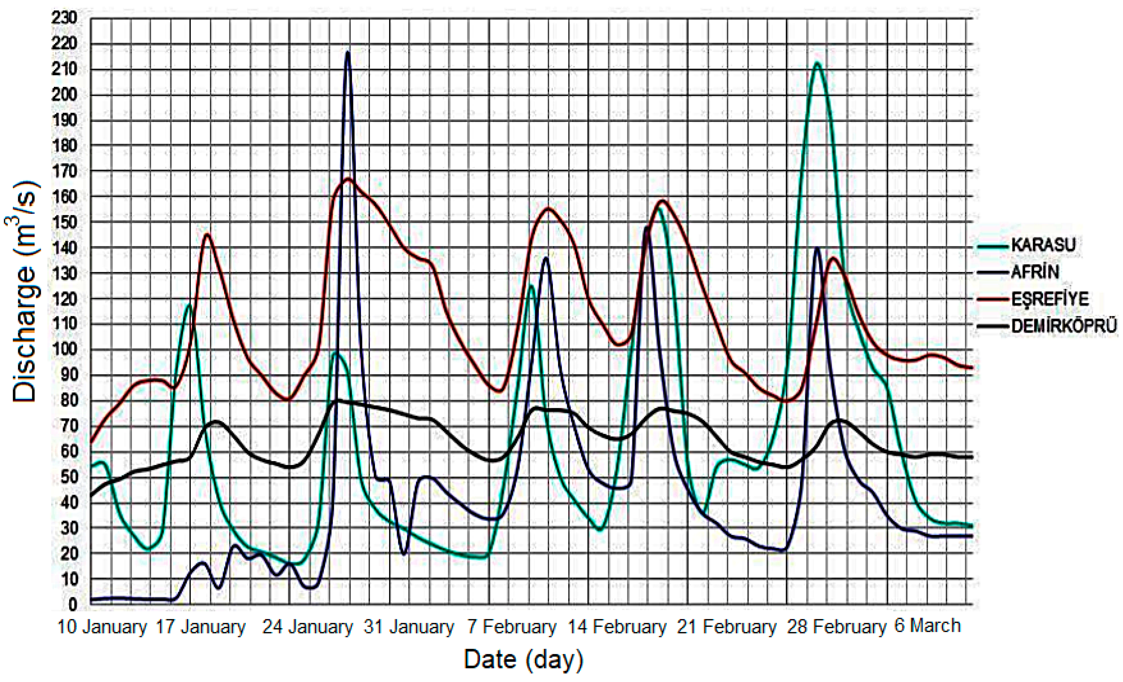
The Amik Plain in the Mediterranean region of Hatay Province is a plain where floods have been experienced in various years. According to the data obtained from the Provincial Directorate of Agriculture, between 27 January and 14 March 2012, rainfall and sudden snow melting caused flooding over a 13,000 ha area on the Amik Plain. A total of 8465 ha of agricultural land, roads, bridges, settlements, and Hatay Airport runway and apron were exposed to flood waters. According to the reports of the Provincial Directorate of Agriculture, the flood damage observed in agricultural lands cost 17,453,161 TL. The Asi River, Karasu stream, Afrin creek, Muratpasa channel, and Comba channel were involved in the floods [3,17]. The flood hydrograph measured at the current observation stations during this flooding is given in Figure 3.
According to this, the highest hydrograph values are observed in the Afrin and Karasu channels.
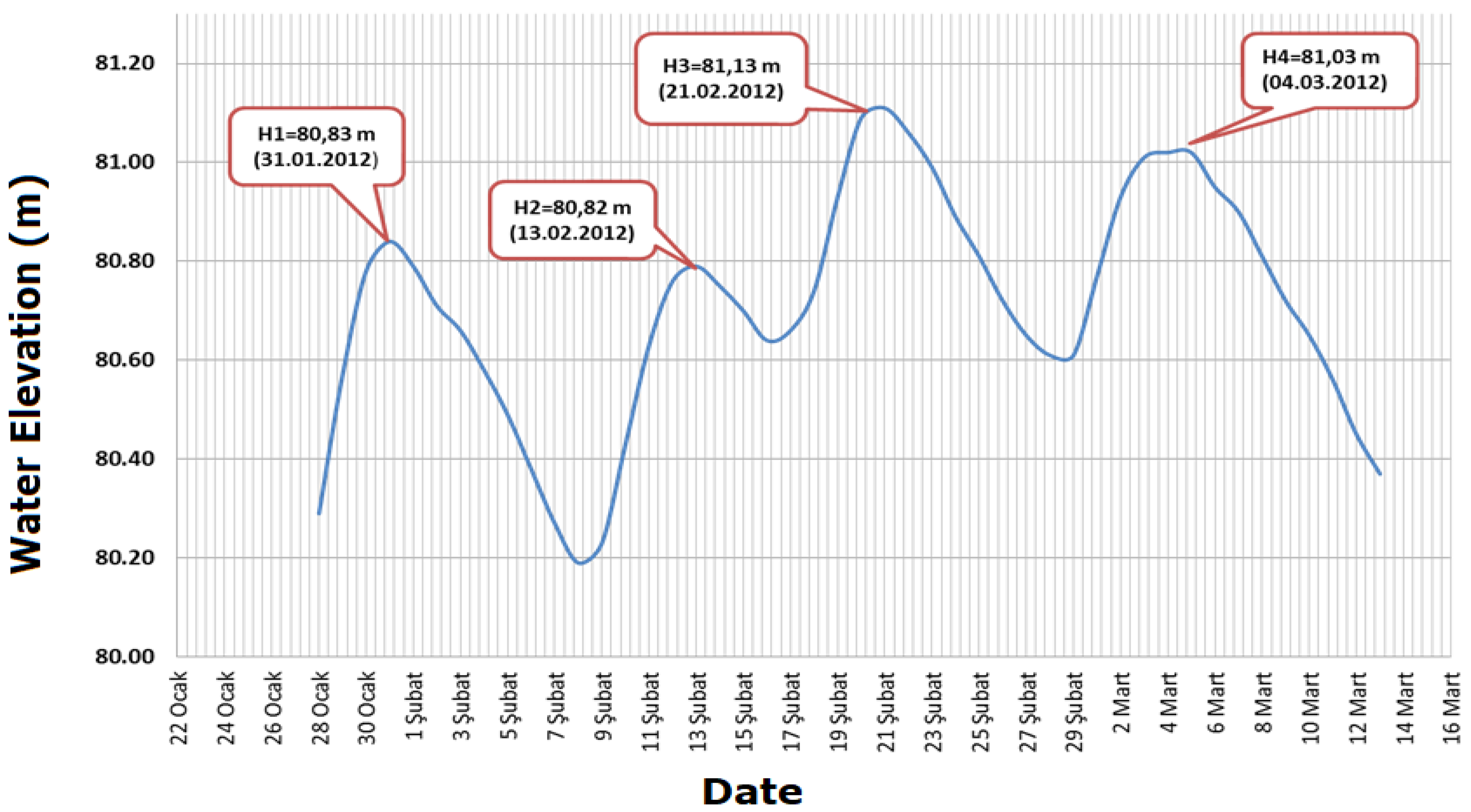
The Amik Plain flood lake elevation hydrograph during this flooding is given in Figure 4. Accordingly, the highest level was measured as 81.13 m on 21 February 2012.
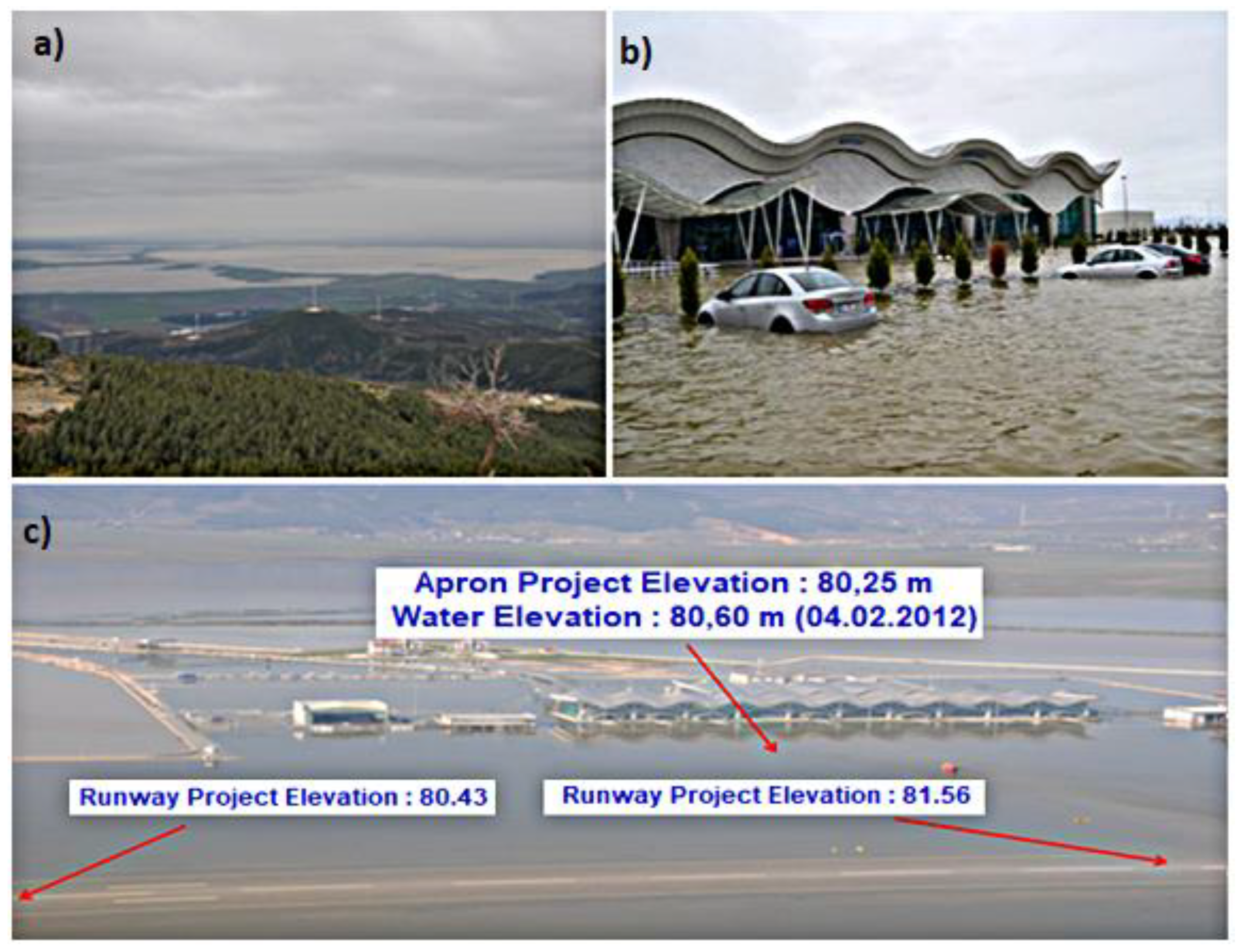
Figure 5 shows the photographs taken of the floods on 2 February 2012. The size and effects of the flooding are clearly visible in the photographs. The apron project elevation and runway elevation of the airport remained below the highest measured lake level.
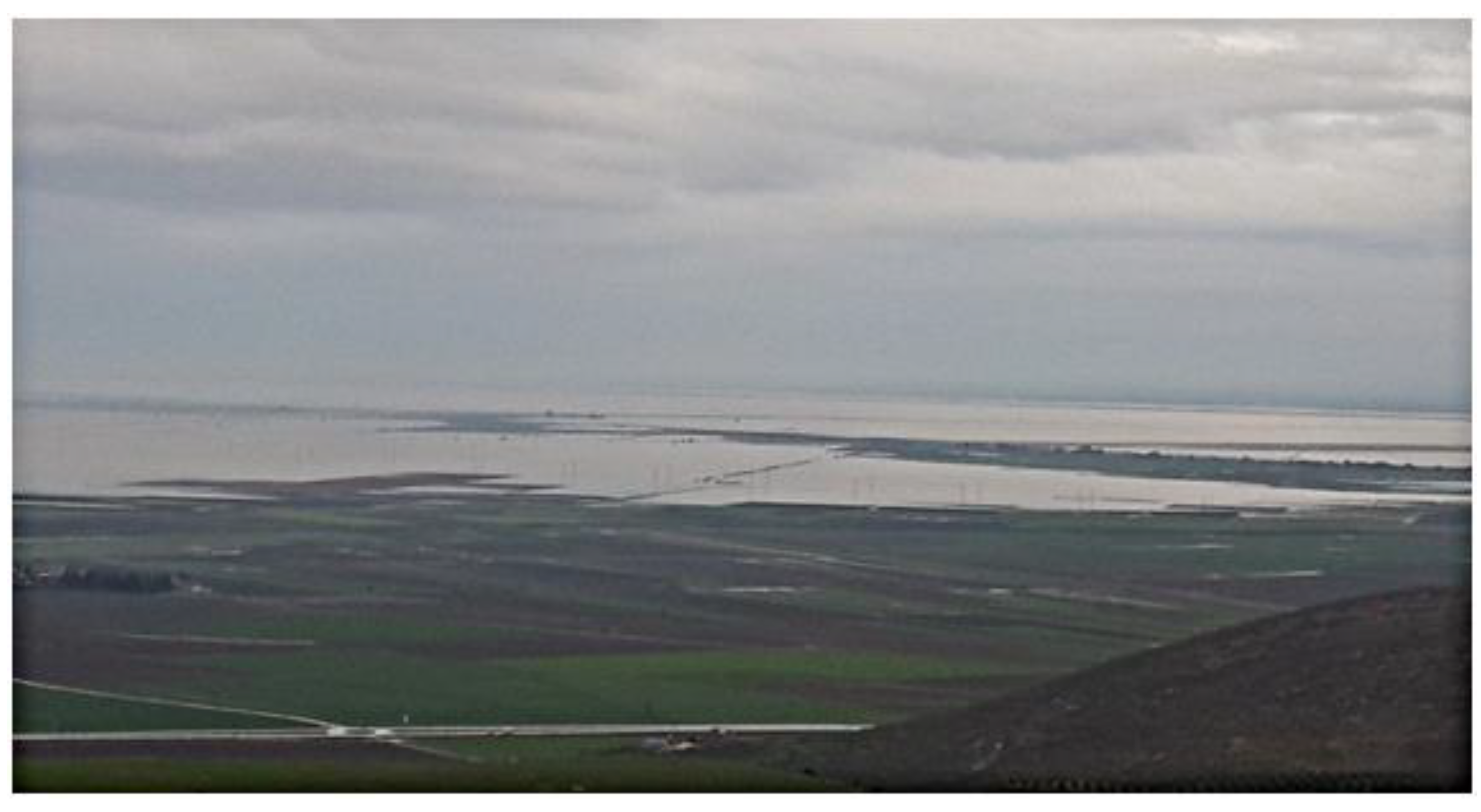
The Amik Plain is flooded almost every year as a result of rainfall. Similarly, as a result of heavy rainfall in February 2019, the water level increased and caused the Amik Plain to be flooded. Figure 6 shows the situation of the Plain in 2019.
2. Model and Application
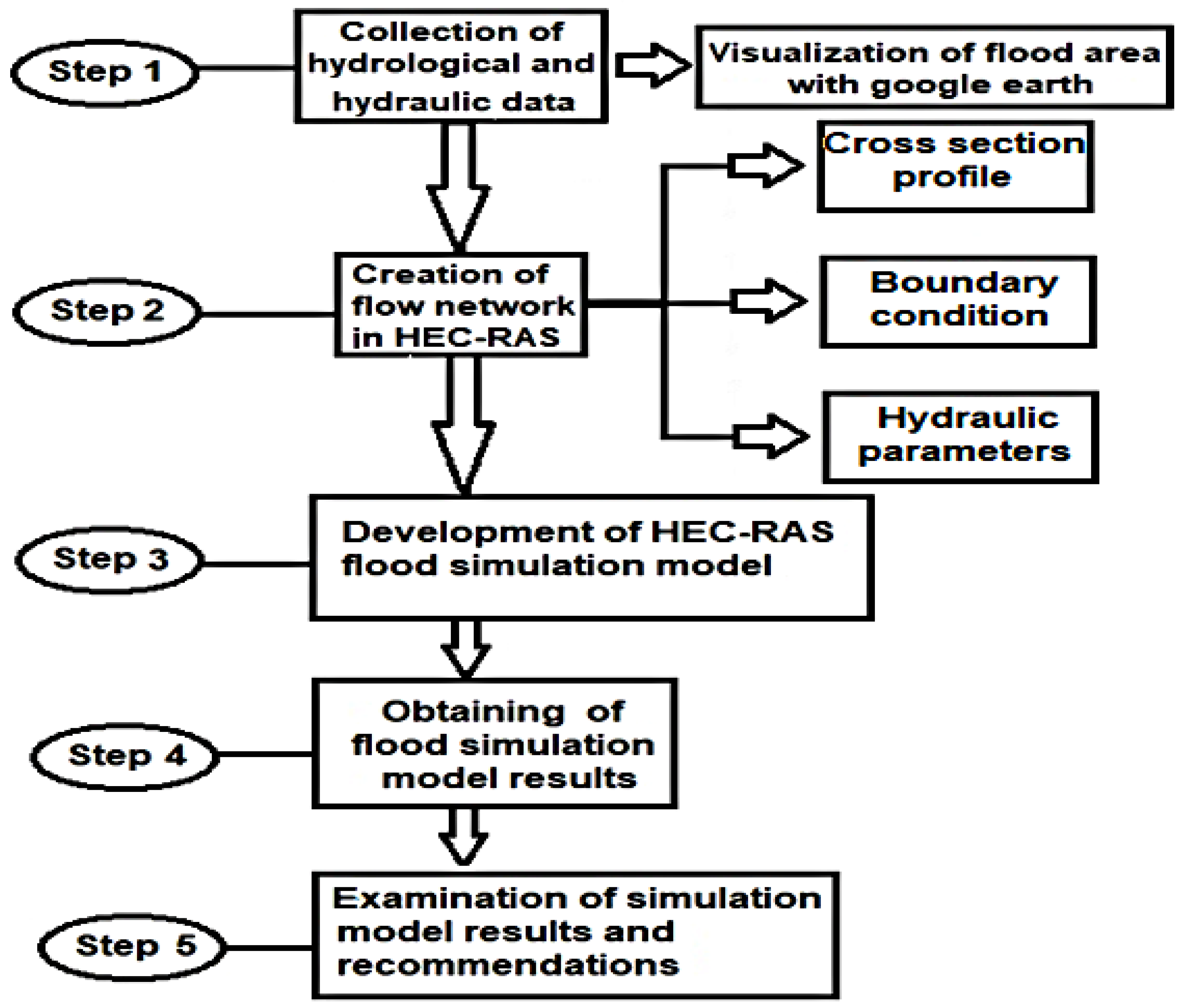
In this study, the HEC-RAS program was used to model flooding. HEC-RAS was developed in 1994 by USACE (United States Army Corps of Engineers). It uses the addition of a graphical user interface (GUI), which differs from the HEC-2 model in the 1970s, for modeling the water profile. The GUI is Windows-based, allowing the user to enter data, correct the entries, and display and get the output of the analysis in an easy format [18,19,20,21]. The flowchart showing the adopted methodology of the program is shown below (Figure 7).
The HEC-RAS package program can perform four different river analyses in one dimension. These include the following:
- Calculation of regular current water surface profiles;
- Varied flow modeling;
- Moving solid boundary sediment transport modeling;
- Water quality analysis studies [21].
For these four approaches, geometric data can be defined in the program and geometric and hydraulic calculations can be made. Regular uniform flow represents the current state in which the flow characteristics do not change depending on the location and time. The main characteristic of the slow changing flow is the slight changes in water depth and speed from one section to another. The HEC-RAS program can solve current problems with subcritical, supercritical, and both.
One-dimensional energy equation is used by HEC-RAS to calculate water surface profiles. With this equation, the following variables are used, the friction coefficient in the Manning equation for energy losses, the kinetic energy correction coefficient for the change in velocity height owing to shrinkage and expansion changes, and the momentum equation where the water surface changes suddenly. In transitions from the river regime to the flood regime (hydraulic jump), the changes in the flow properties caused by the bridges and the analysis of the flow properties formed in the cross-sections of the rivers are also solved using these equations.
2.1. Basic Equations for Profile Calculation
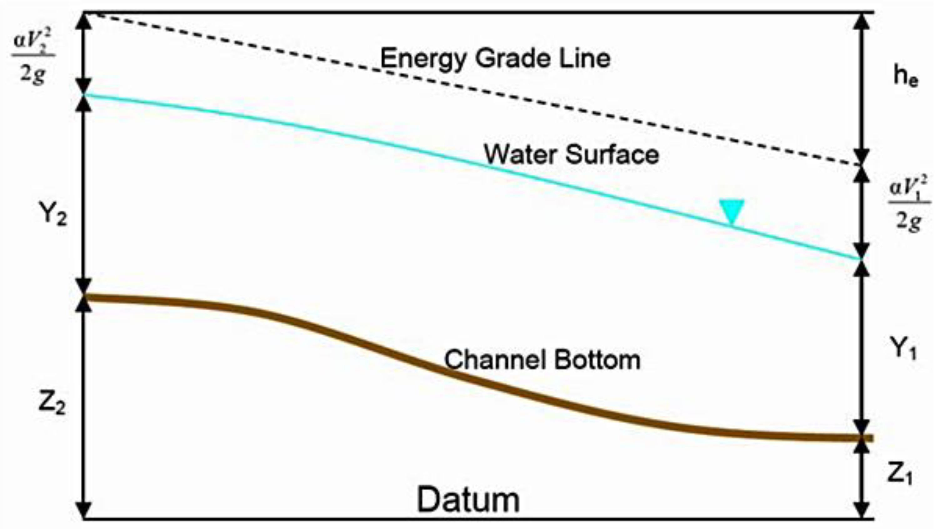
Water surface profiles are calculated from one section to another by the method named as the standard step method based on the repeated solution of the energy equation. The energy equation can be written as follows and given Figure 8:
where z1, z2, main channel bottom height (m); Y1, Y2, sectional flow depth (m); V1, V2, mean velocity (m/s); α1, α2,velocity coefficients; g, gravitational acceleration (m/s2); and he, energy loss height (m). The energy loss between two sections (he) consists of friction loss and contraction or expansion loss. Energy head loss is defined by the following expression:
where L, channel length; Sf, friction slope between two sections; and C, expansion or contraction loss coefficient.
L channel length is calculated as follows:
where Llob, Lch, Lrob, flow way length, left flood plain, main channel, and right flood plain;
Qlob, Qch, Qrob, mean discharge between sections, left flood channel, main channel, and right flood channel.
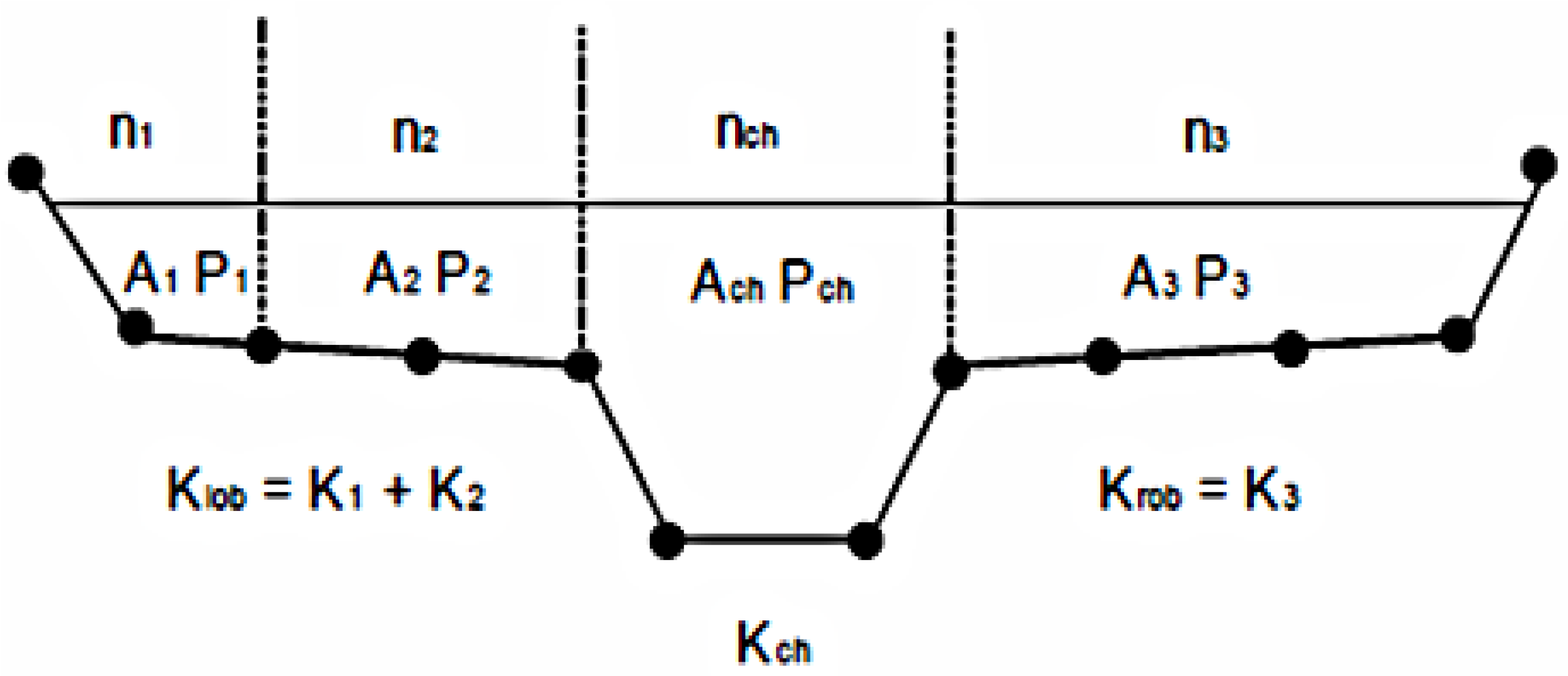
2.2. Transmission Calculation of Section Subdivisions
In order to determine the total flow rate and velocity coefficient in a cross section, the cross section of the channel must be subdivided where the distributions are uniform. HEC-RAS considers the roughness (n) changes on main channel and flood channel to subdivide the cross sections as shown in Figure 9. The transmission capacity for each sub-region is calculated with the Manning formula given below.
where K, transmission capacity for each sub-region; n, Manning roughness coefficient for each subregion; A, bottom sectional area; and R, bottom section hydraulic radius.
The program collects the transmission capacities of subfields on the right and left coasts to calculate the total transmission capacity and the transmission capacities of the main channel, which are usually taken as a single part.
2.3. Head Loss Calculation
In HEC-RAS, friction loss is calculated with the help of the friction gradient Sf and the length L, given by Equation (3). The friction slope (slope of the energy line) in each section is calculated from the Manning equation as follows.
2.4. Determination of Contraction and Expansion Loss
Contraction and expansion losses in HEC-RAS are calculated with the help of the following equation:
where C is the contraction or expansion coefficient.
The software accepts that, if the speed load at the downstream is greater than that at the upstream, the expansion occurs when the speed load at the upstream is greater than at the downstream. Sample values for the C coefficient are given in Table 1 below.
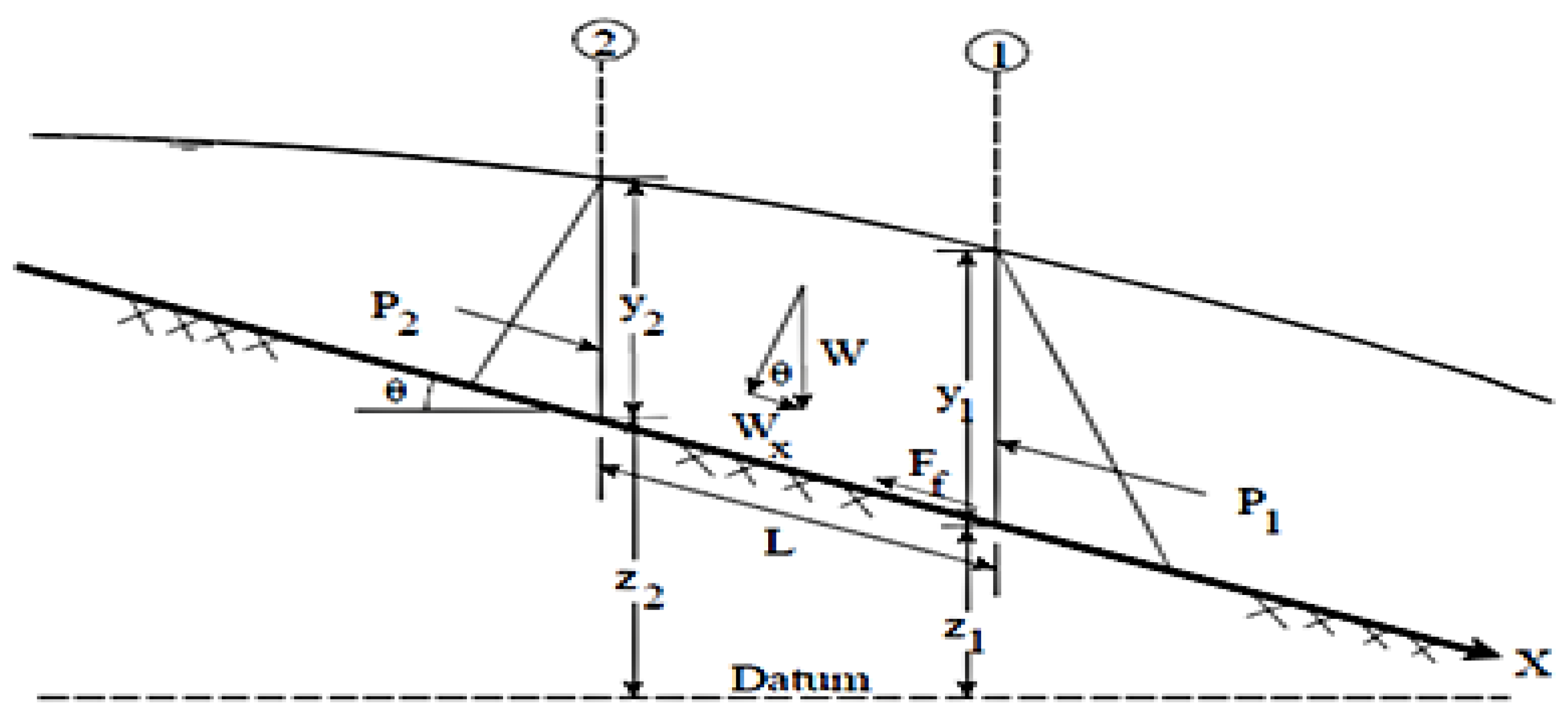
The program tries to determine the water surface profile using the above equations with repeated solutions and limits the maximum number of iterations to 20 to balance the water surface. While the program uses the energy equation for regular currents, it uses the momentum equation in varied flow. In many flow situations, there is a transition from supercritical to subcritical or to subcritical to supercritical. This situation occurs in sections, bridge structures, fall structures and sluices, and flow joints, which are important changes in channel slope. The momentum equation is derived from Newton’s second law of motion as follows and given Figure 10:
where Fx, force; m, mass; and a, acceleration.
If we apply Newton’s second law of motion to the flow segment between Section 1 and Section 2, the momentum change in unit time can be written as follows:
where , 1 and 2 hydrostatic pressure force in cross sections; , the x component of the weight force; Ff, friction loss between Section 1 and Section 2; Q, discharge;, specific mass of water; and , the change in velocity between points 1 and 2 in the x direction.
After performing the necessary intermediate operations, the shape of the momentum equation used by the software can be obtained.
An important term used to determine the regime of the flow, that is, subcritical and supercritical flow in varied flows using the momentum equation, is the Froude number and is expressed as follows.
where V, flow velocity; g, gravity acceleration; and h, flow depth. If Fr = 1, it is defined as critical current, Fr < 1, it is defined as subcritical current, i.e., river regime, and if Fr > 1, it is defined as supercritical current, namely flood regime.
2.5. Manning Coefficient for Main Channel
If the main channel roughness does not change, the section is not subdivided and the calculation is made by considering a single n value. If the main channel roughness is variable, HEC-RAS checks the compatibility of the roughness of the main channel sub-parts, and if necessary, calculates a single equivalent roughness coefficient of the entire section.
It is important to determine the appropriate Manning coefficient for the accuracy of the calculated water surface profiles. Manning n value is highly variable and depends on many factors; surface roughness, plant properties, channel irregularity, channel horizontal slope, meandering, scouring and accumulation, obstacles, channel shape and size, flow, seasonal changes, temperature, hangers, and swabs.
In the case in which there is water surface information of a cross section, the Manning value (n) can be calibrated. If there is no such information, similar current conditions or value obtained by experimental studies can be used for the n value. There are many sources for determining the value of Manning n for different channel properties. The broadest information for the value of “n” in streams and flood channels is given in Chow’s Open Channel Hydraulics (1959) [22]. The information from this book is given in Table 2. The model can be calibrated with the n values of streams that are presented in the book and presented with pictures.
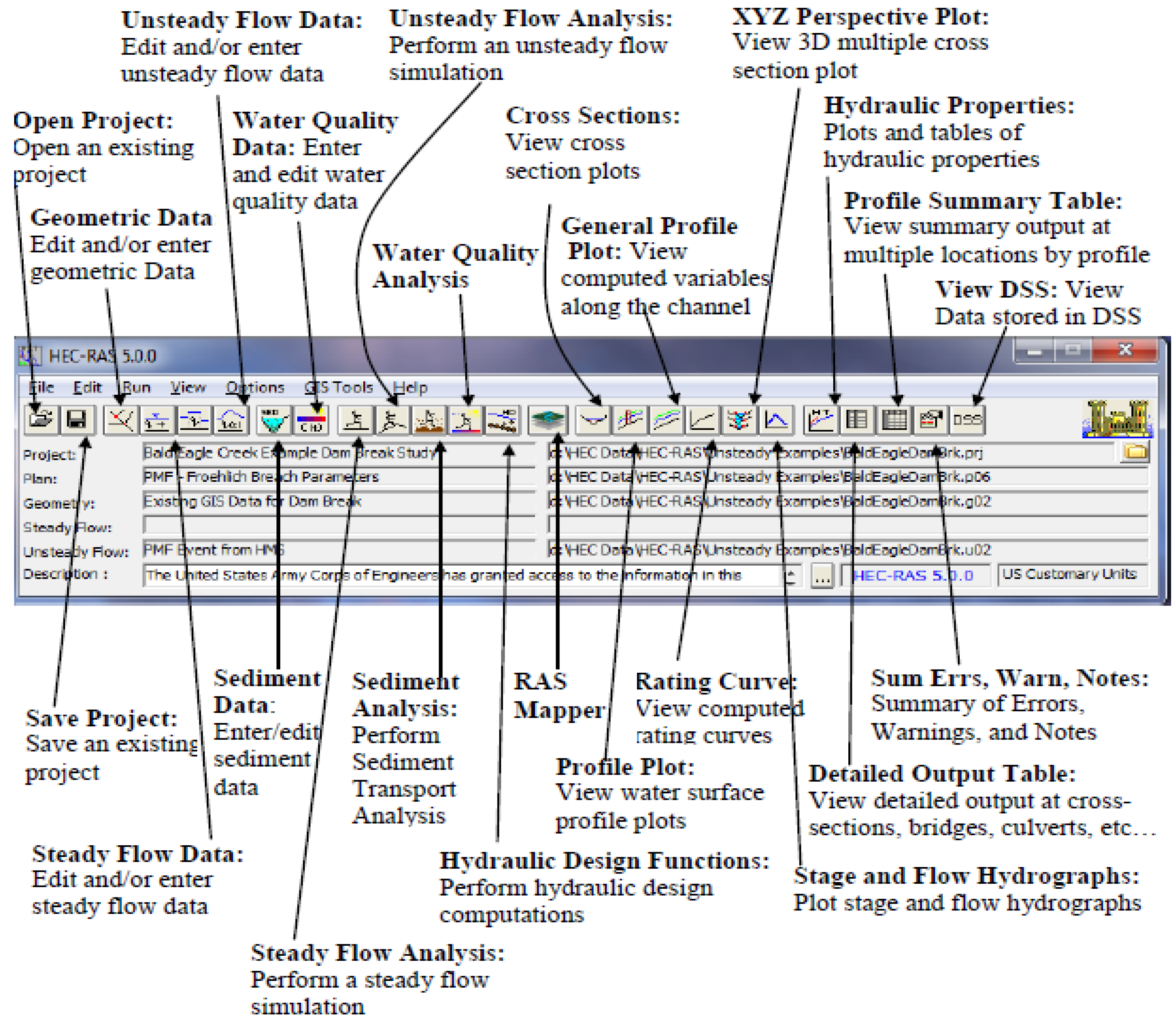
2.6. HEC-RAS Software Buttons
When the program is first opened, the function of the buttons in the window is shown in Figure 11. For more information, the user’s guide can be read.
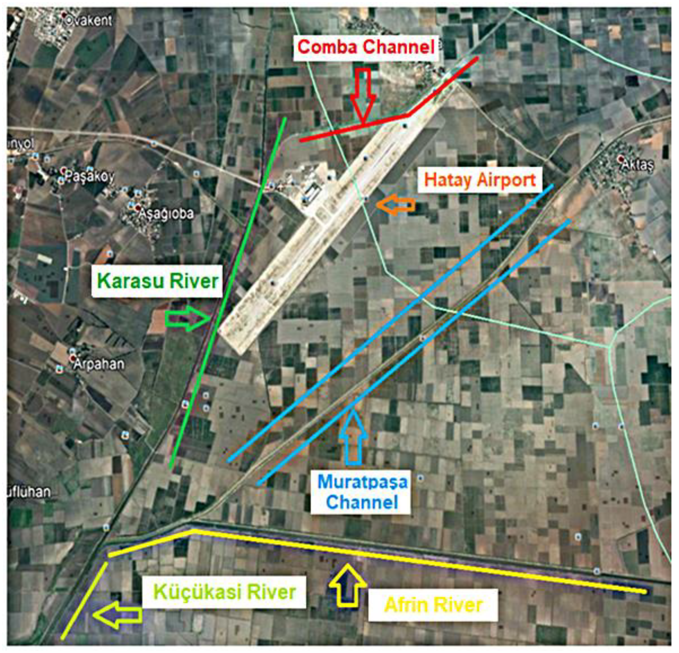
2.7. Creating Geometric Data
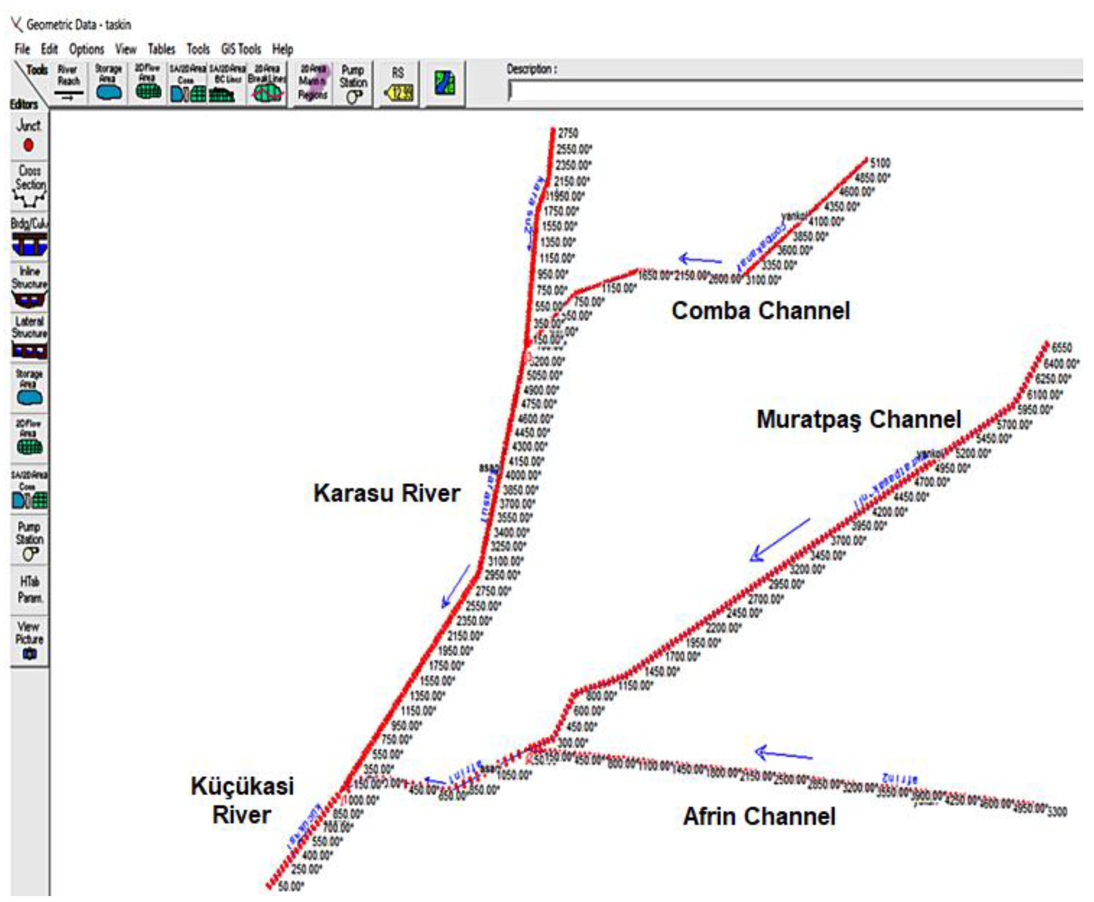
In this study, the geometric model of the flooding, the maps of the Amik Plain, and the channels and rivers seen in Figure 12 were digitized as accurately as possible using the Google Earth software [23].Parts of the Küçükasi River (1050 m); Karasu River (8050 m); and the Comba, Muratpaşa, and Afrin channels (5100 m, 6550 m, and 6600 m, respectively) are modeled and a cross-section of every 50 m is formed. The drawing of the river network was created with the sections in the window that came in by clicking the Geometric Data icon in the main menu of HEC-RAS, shown in Figure 11 and Figure 13. The HEC-RAS model of channels and cross-sections is presented in Figure 13.
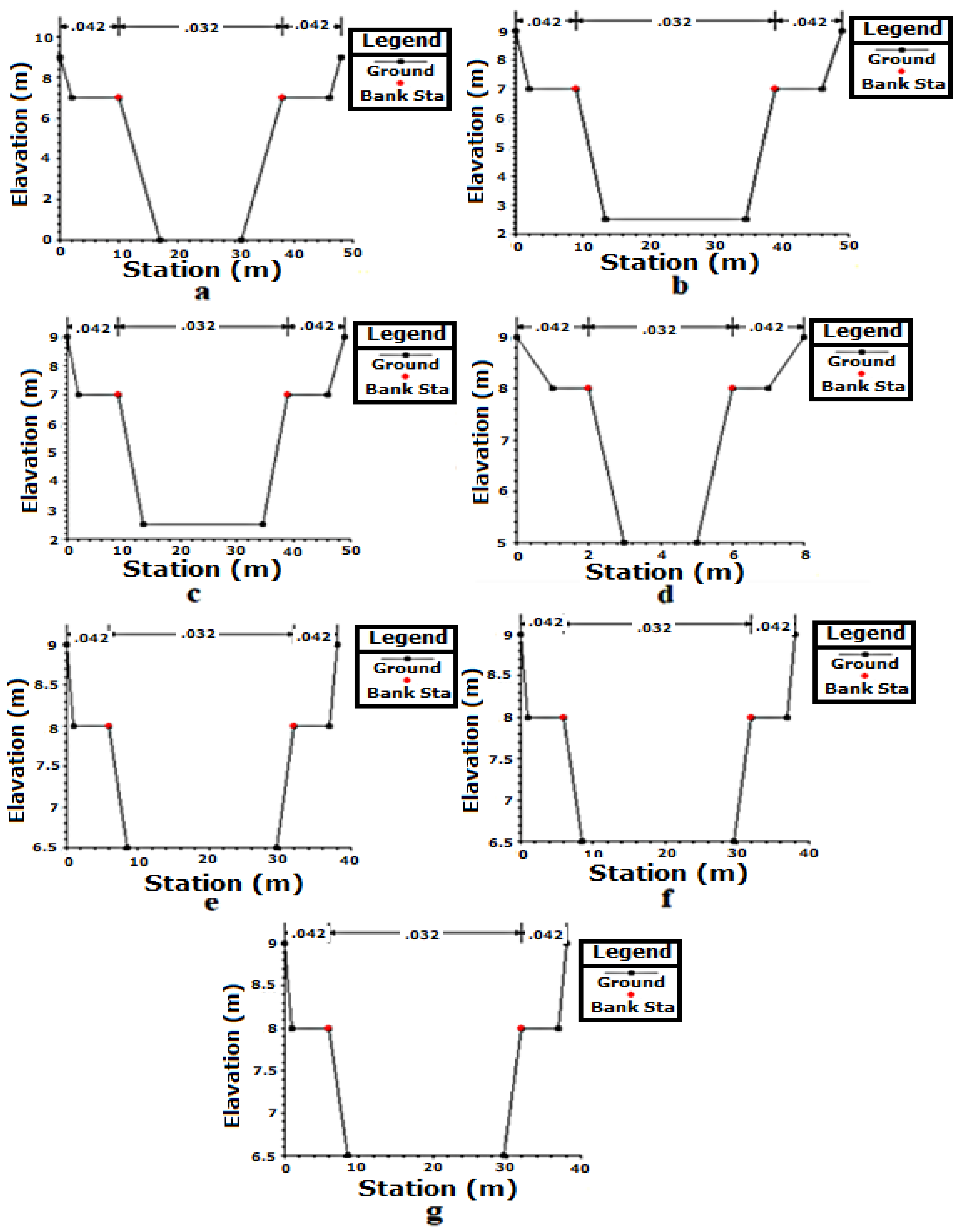
The lowest elevation levels in the numerical model were measured on the Küçükasi River +81 m, Karasu River +79 m, Afrin channel +79 m, and the Muratpasa and Comba channels +78 m. Afrin and Karasu are formed from two parts, considering the intersection points where the flow network was created. The sections of the flow paths were formed by entering data into the program similar to the cross-section values specified by the DSI in the flood report. Figure 14 shows these sections. There is a slope of 0.1% in the formed current networks. On the basis of the authors’ field observations, water organization reports, and Google Earth software, the authors saw that channels exist generally from natural soil, and that is why the Manning coefficient used for the study is considered as 0.042 for both sides of the channels and 0.032 for the bottom of channels. The Manning coefficient is selected in accordance with the regional conditions according to the information in Table 2.
2.8. Hydraulic Analysis
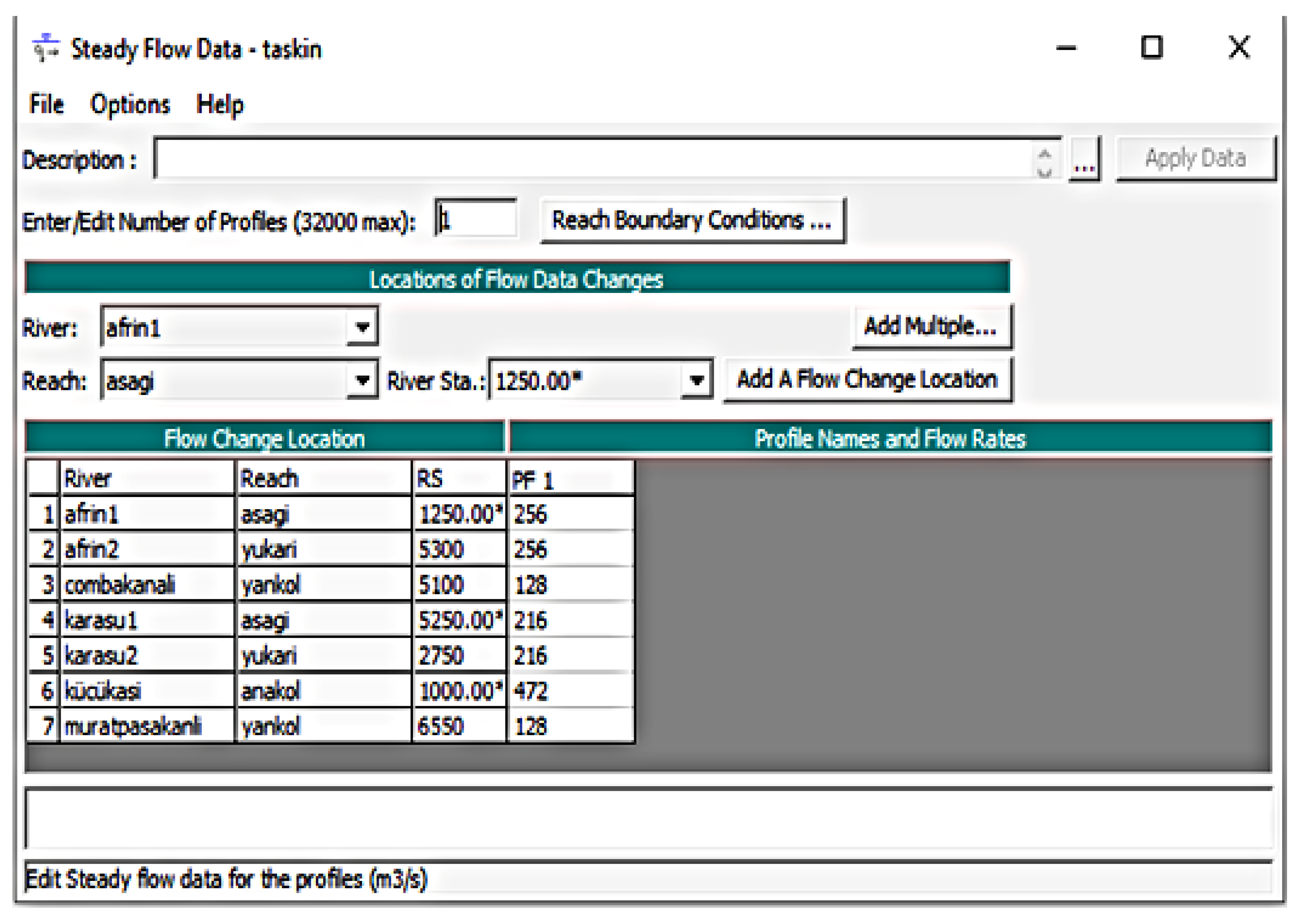
The steady flow icon is selected from the main bar and the window in Figure 15 appeared. After the geometric model was generated, the values measured at the flow observation stations during the flooding were entered into the program, as shown in Figure 15. These values were taken from the DSI flood report. On the basis of the available data, the model was run for steady flow conditions and the results were examined in accordance with this situation.
3. Results
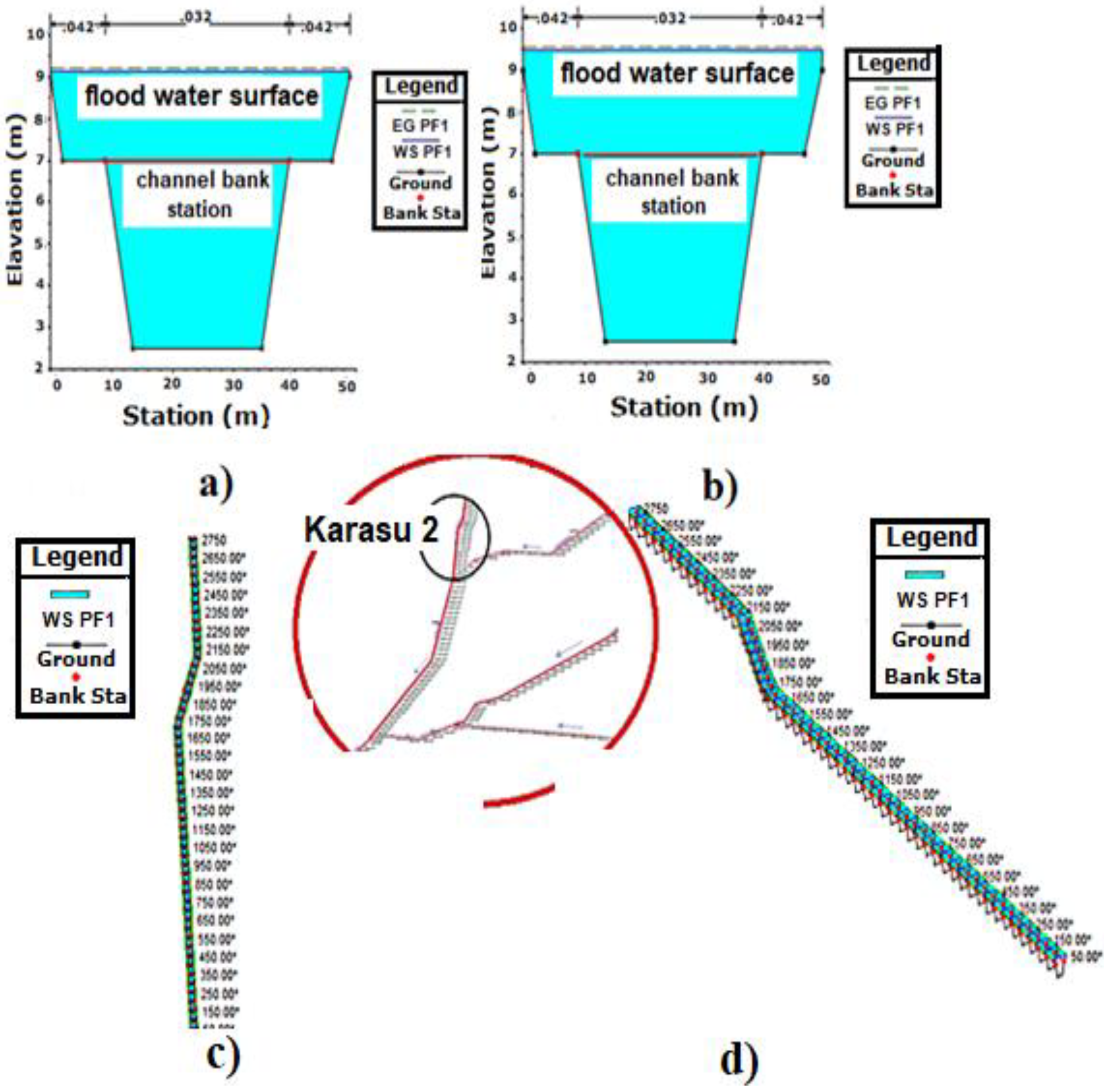
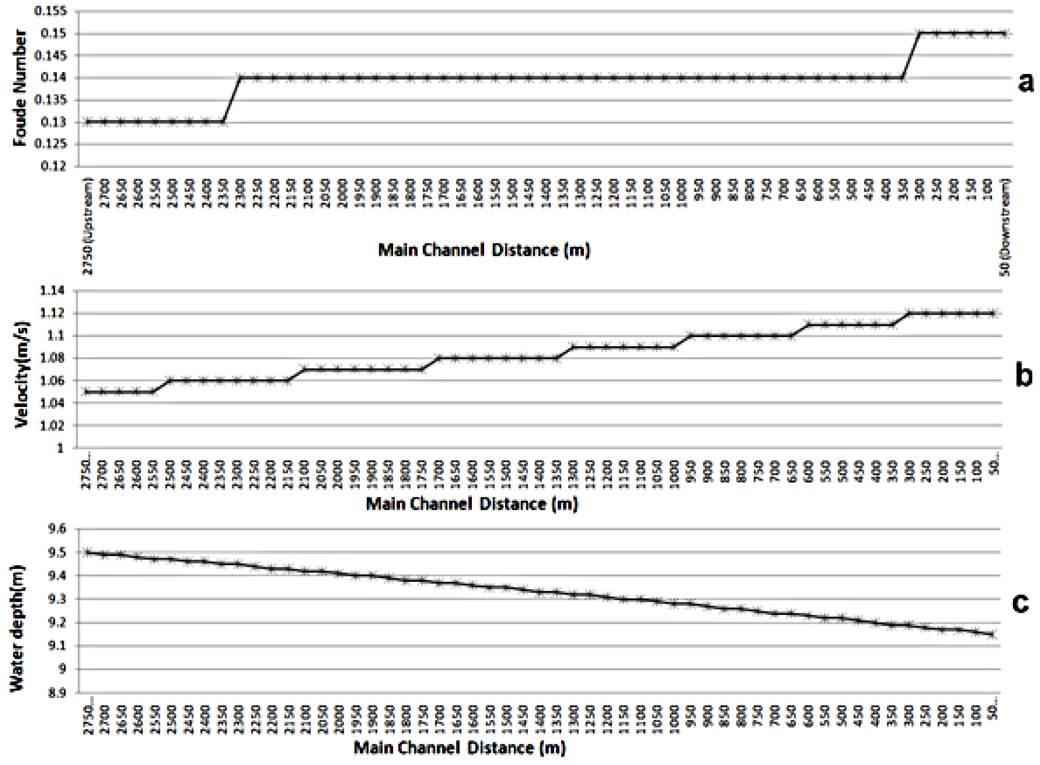
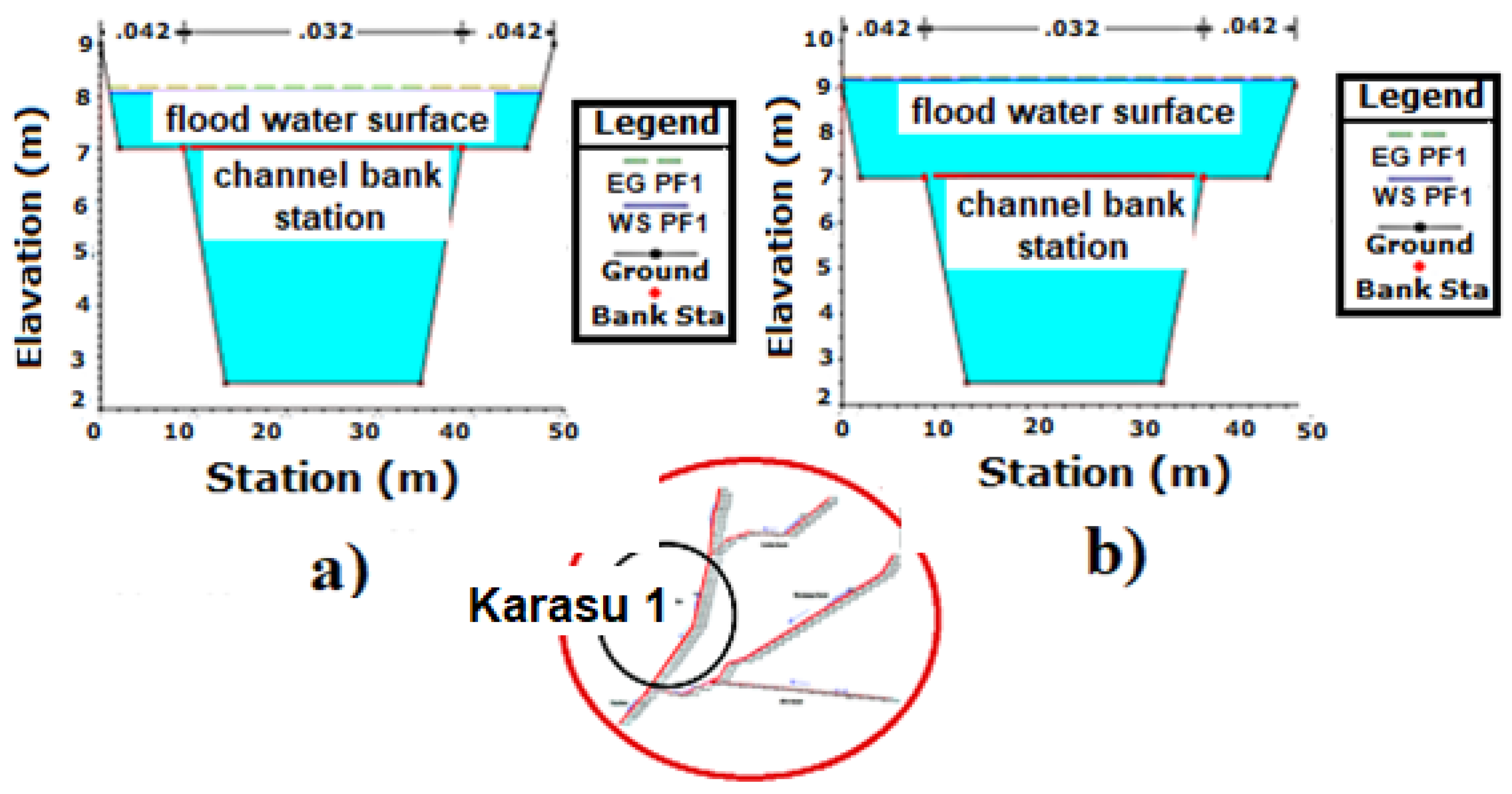
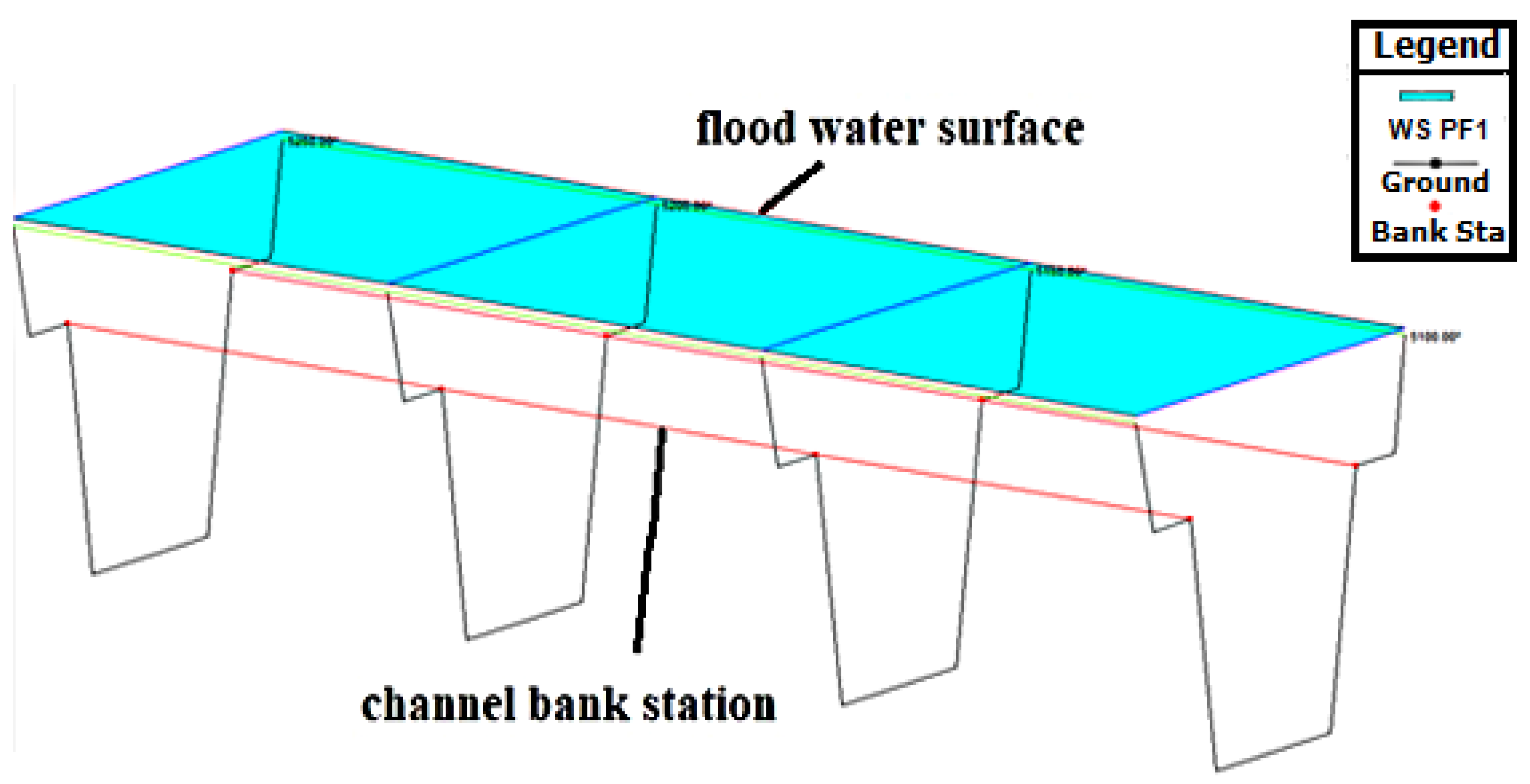
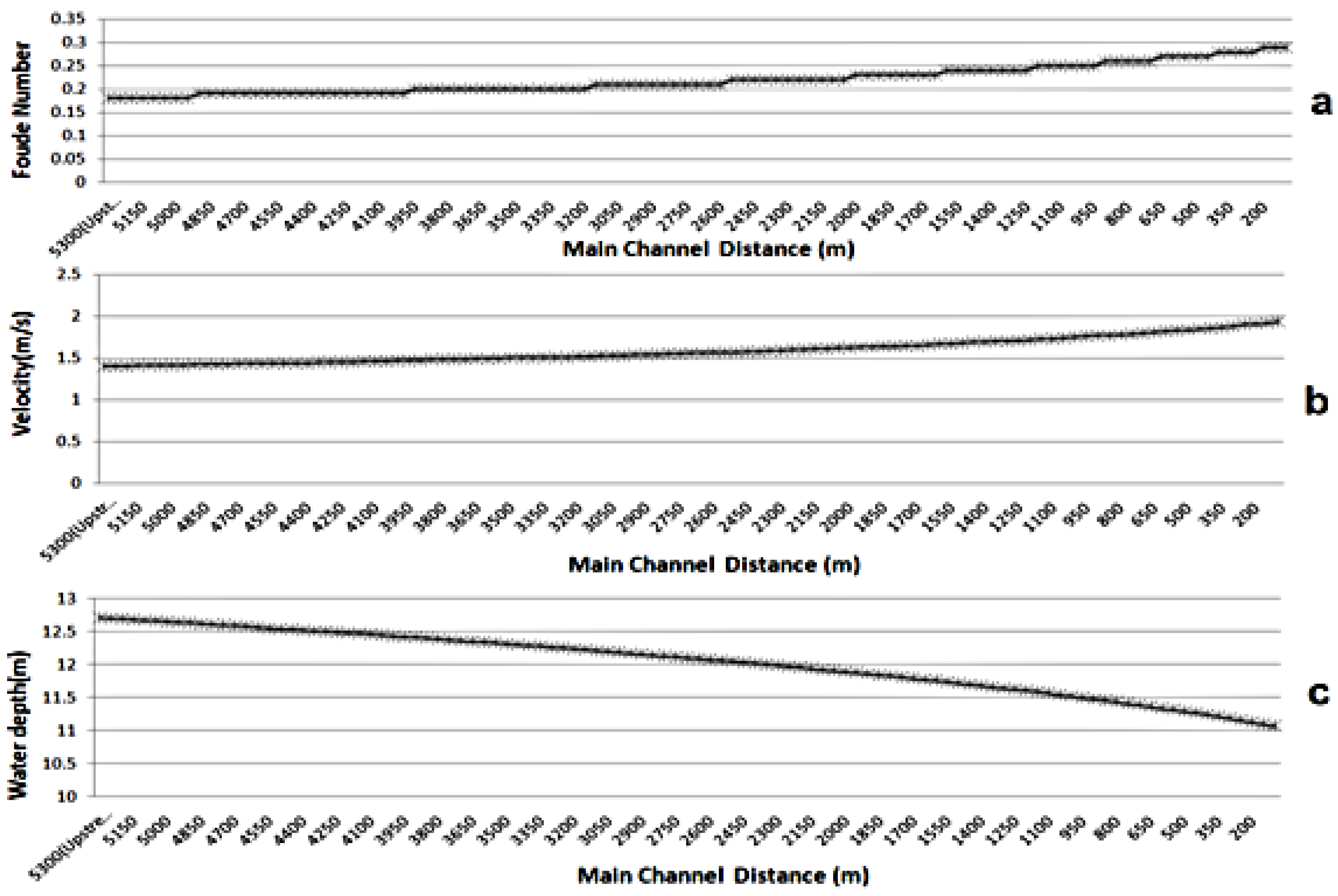
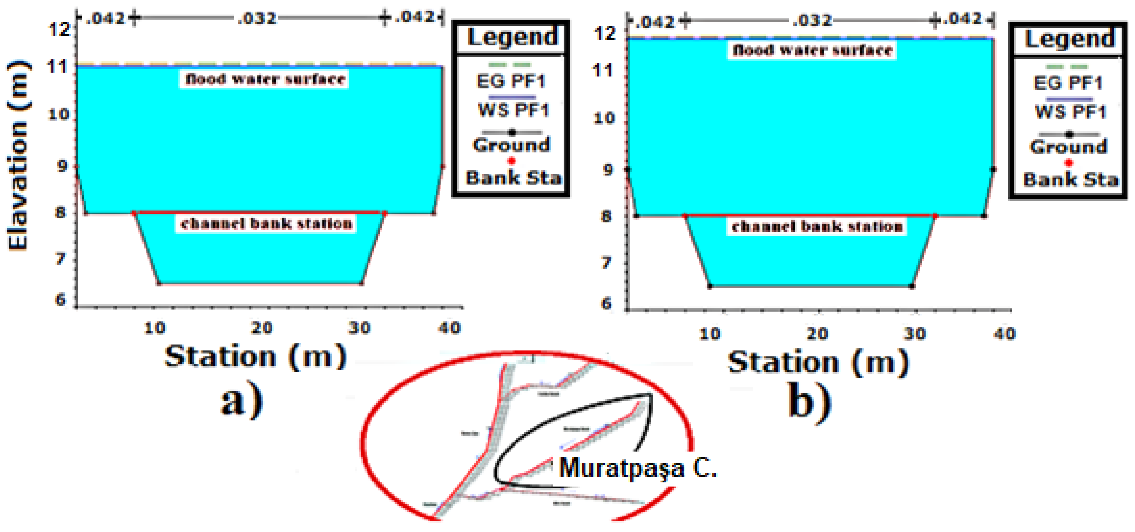
The results of the flow network were analyzed separately for each branch, and the following benefits were obtained. As seen in Figure 16a,b, for the flow of Q = 216 m3/s, the first (50 m) and the last (2750 m) sections of the second part of the Karasu river were flooded about 2.5 m above the upper elevation of the channel. Figure 16c,d show perspective views of the flow from two sides for all sections. Figure 17a–c graphically show the change in the Froude number, speed, and water depth change along all sections for the second part of the Karasu river. When the graphs are examined, it is seen in Figure 17a that the Froude number indicates that the flow is sub-critical across all sections, that is, for the standard river regime, and there is a slow rise from upstream to downstream. Figure 17b indicates a slow increase in the flow rate as well as in the Froude number plot. Figure 17c shows that the water depth decreases slowly as the flow rate increases from upstream to downstream. Because the simulation operates in steady flow conditions, the HEC-RAS program keeps the discharge value constant, and thus water depth decreases with increasing velocity values.
As seen in Figure 18, water depth is one meter above the first part of the Karasu river section (first 50 m) and is two meters above the second part (last 5250 m) of the Karasu river section. Figure 19 shows perspective views of the last four sections of the parts between 5100 and 5250 m.
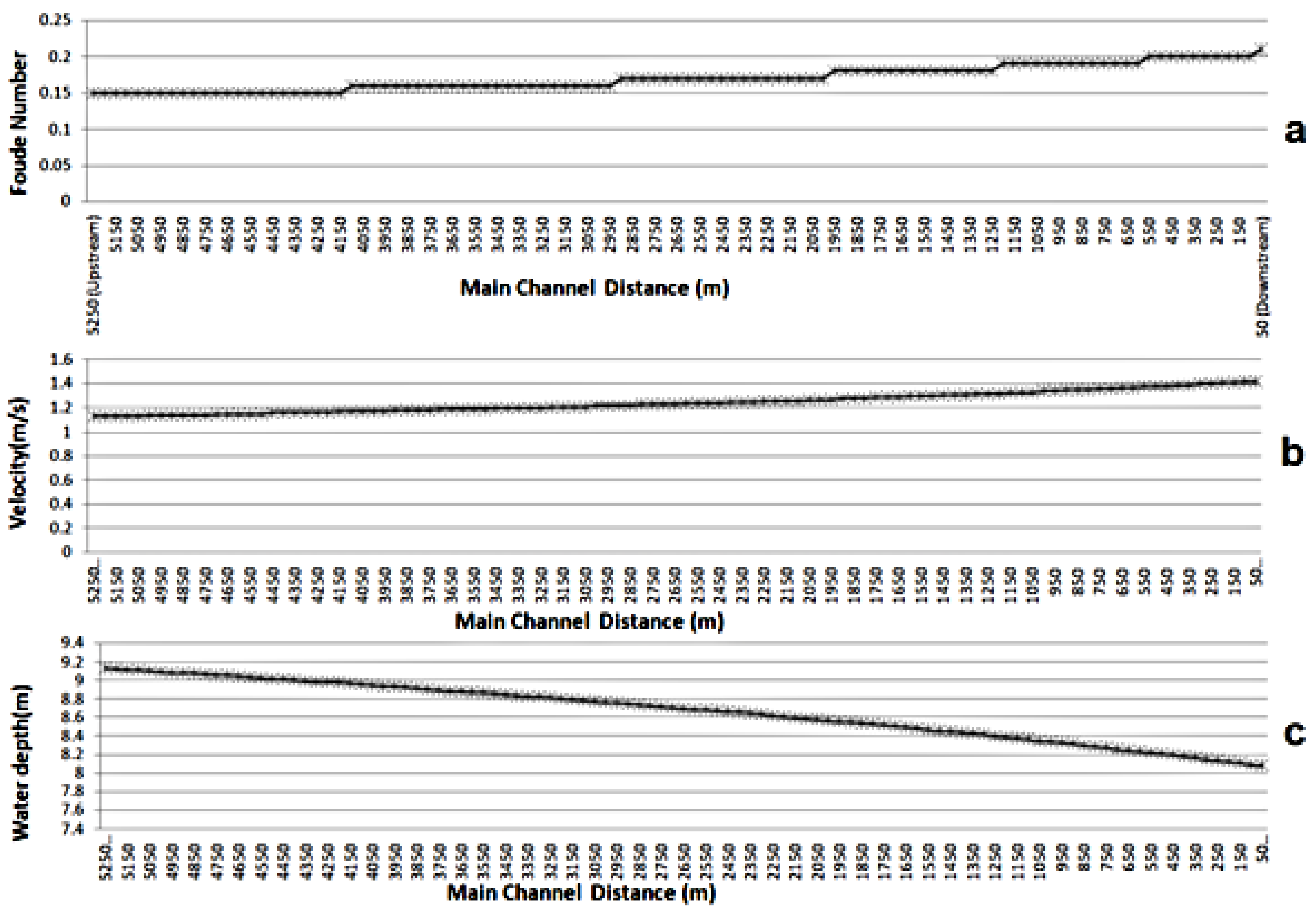
Figure 20a–c show the changes in the Froude number, velocity, and water depth along all the sections in the first part of the Karasu River. A similar situation is also observed in the second part of Karasu River. Froude number and velocity increase slowly, but the water depth decreases.
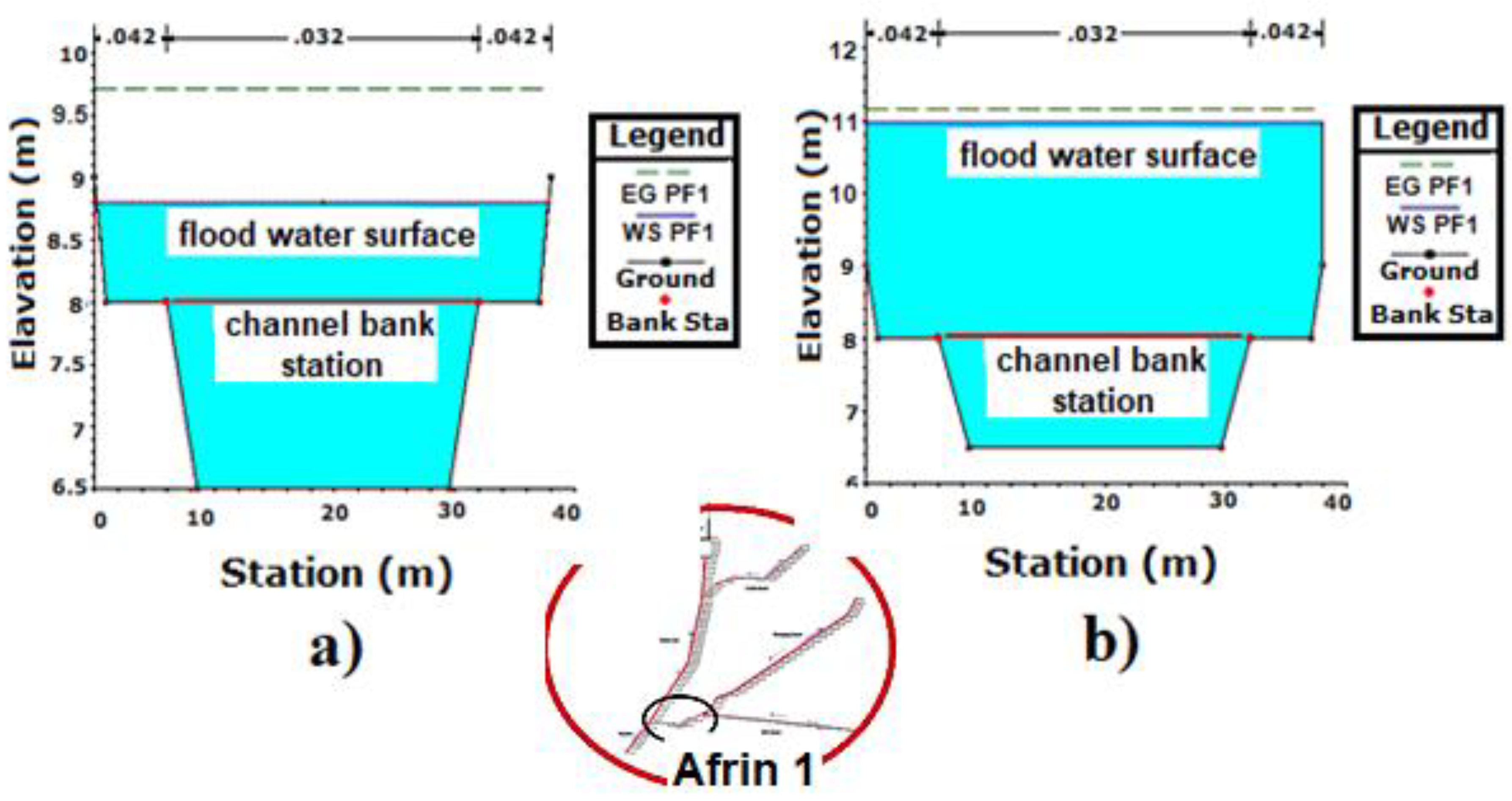
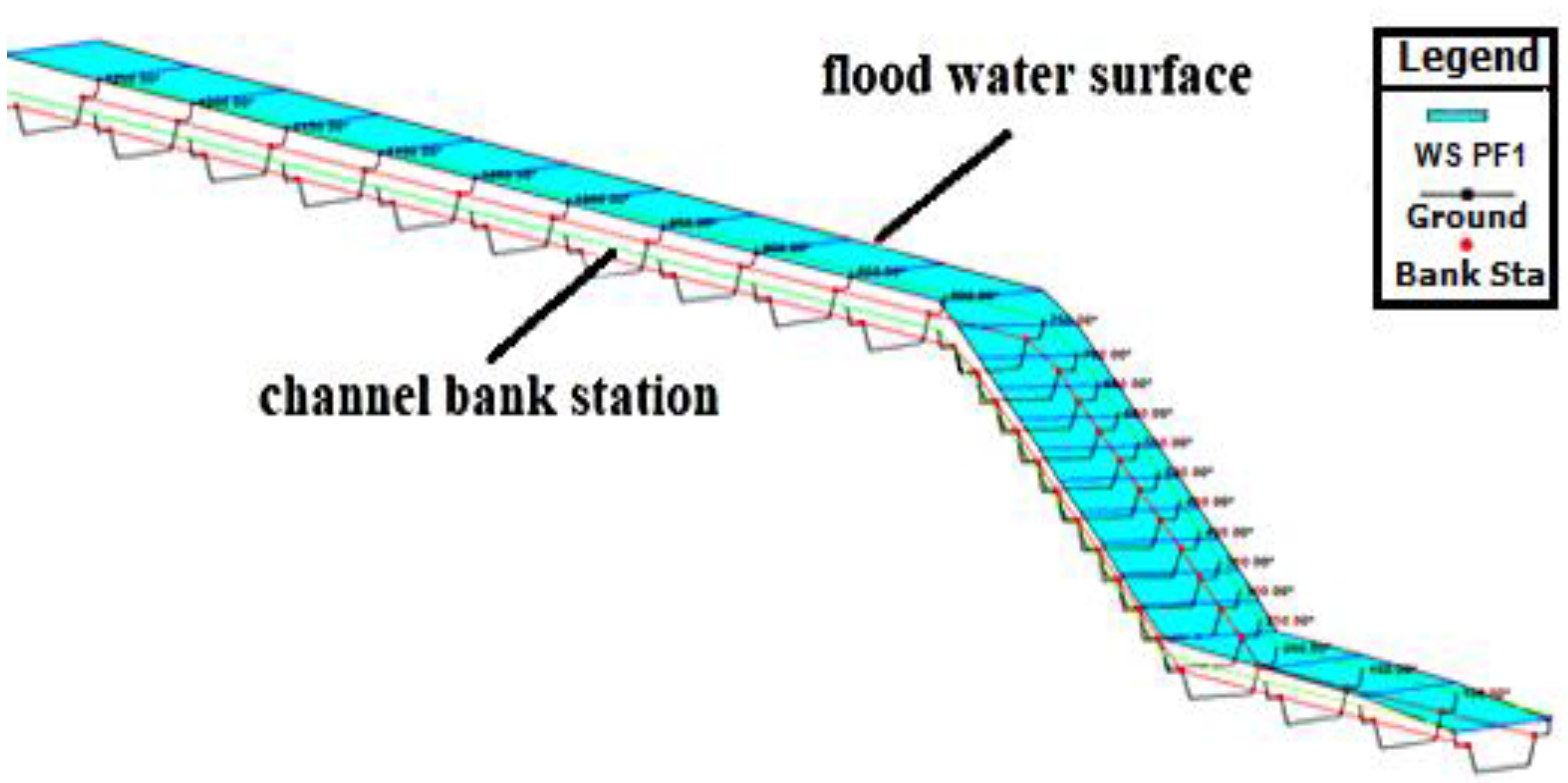
Figure 21a,b relates to the Afrin channel analyses. It is understood from these figures that, when the discharge is Q = 256 m3/s, the water level is approximately two meters above the channel banks for the first part of the Afrin channel (first 50 m), and it is approximately three meters above the banks for the last 1250 m. Figure 22 shows a perspective view of the flow for all sections.
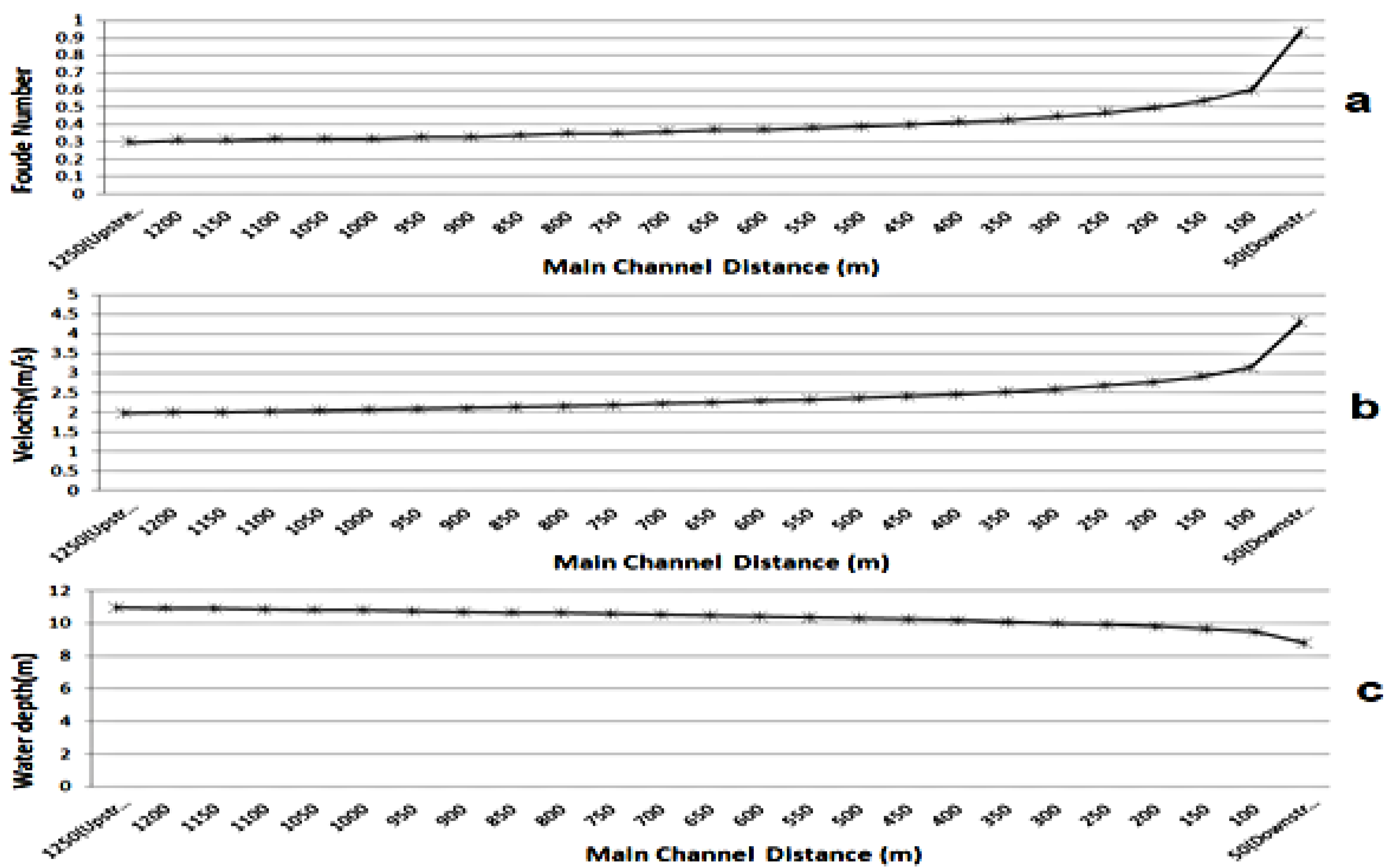
Changes in Froude number, velocity, and water depth are shown for the first part of the Afrin channel and graphs relating to them are presented in Figure 23. When the graphs are examined, it is seen that the Froude number increases rapidly, from a value of about 0.3 upstream and approaching 1.0 (critical value) further downstream. Similarly, the velocity value rises to 4.5 m/s from 2 m/s. This change causes an increase in water depth of about 2 m.
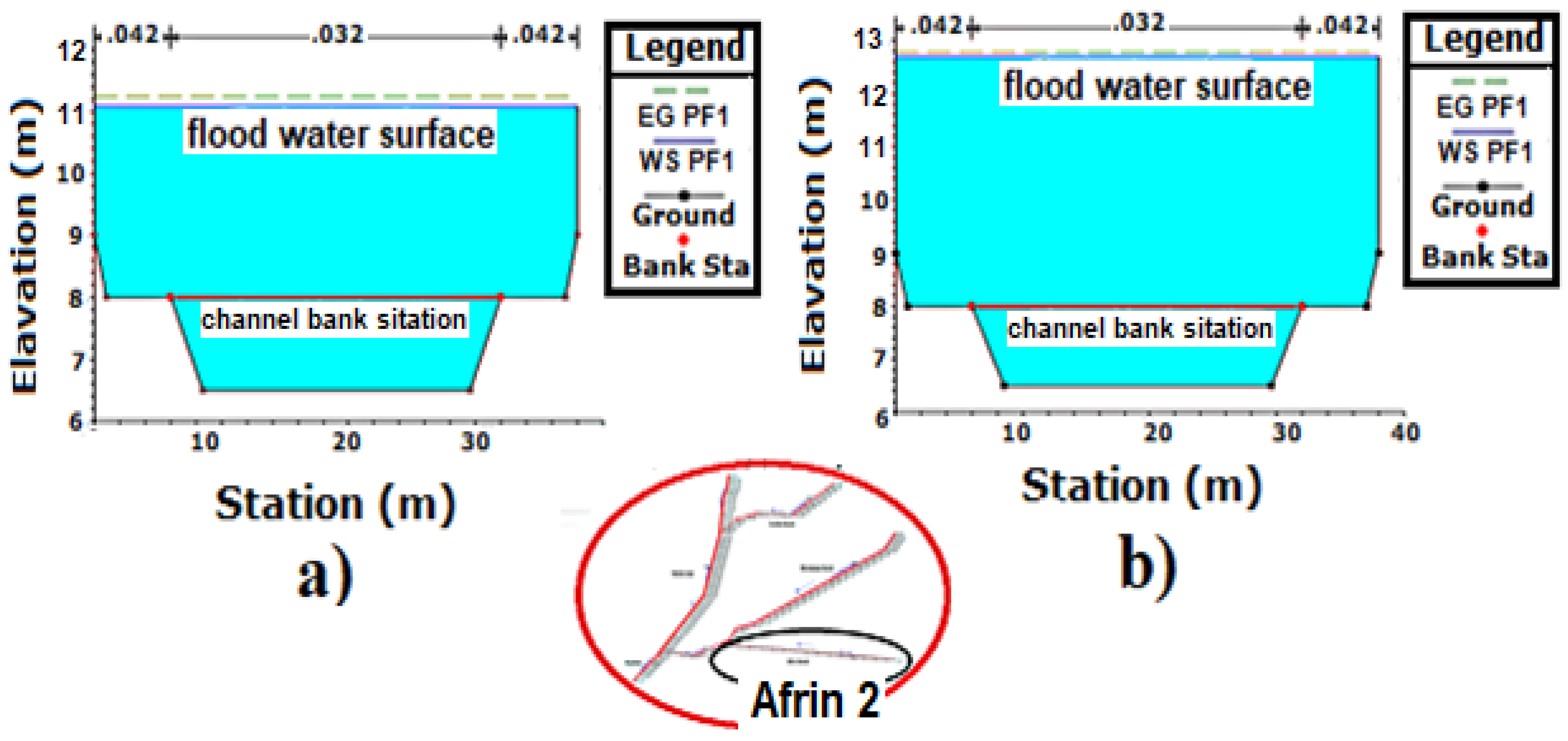
Figure 24 shows that, at discharge Q = 256 m3/s in the Afrin channel second part, flooding occurs three meters above the channel section top height in the first 100 m and five meters above the channel section top height in the last 5300 m. Figure 25 shows perspective views of the last five sections between 5100 and 5300 m.
Figure 26a–c shows a slow increase in the Froude number when the graphs are examined along all the sections in the second part of the Afrin channel. Likewise, the velocity value increases from 1.5 m/s to 2 m/s. This increase causes a change in water depth of about 1.5 m.
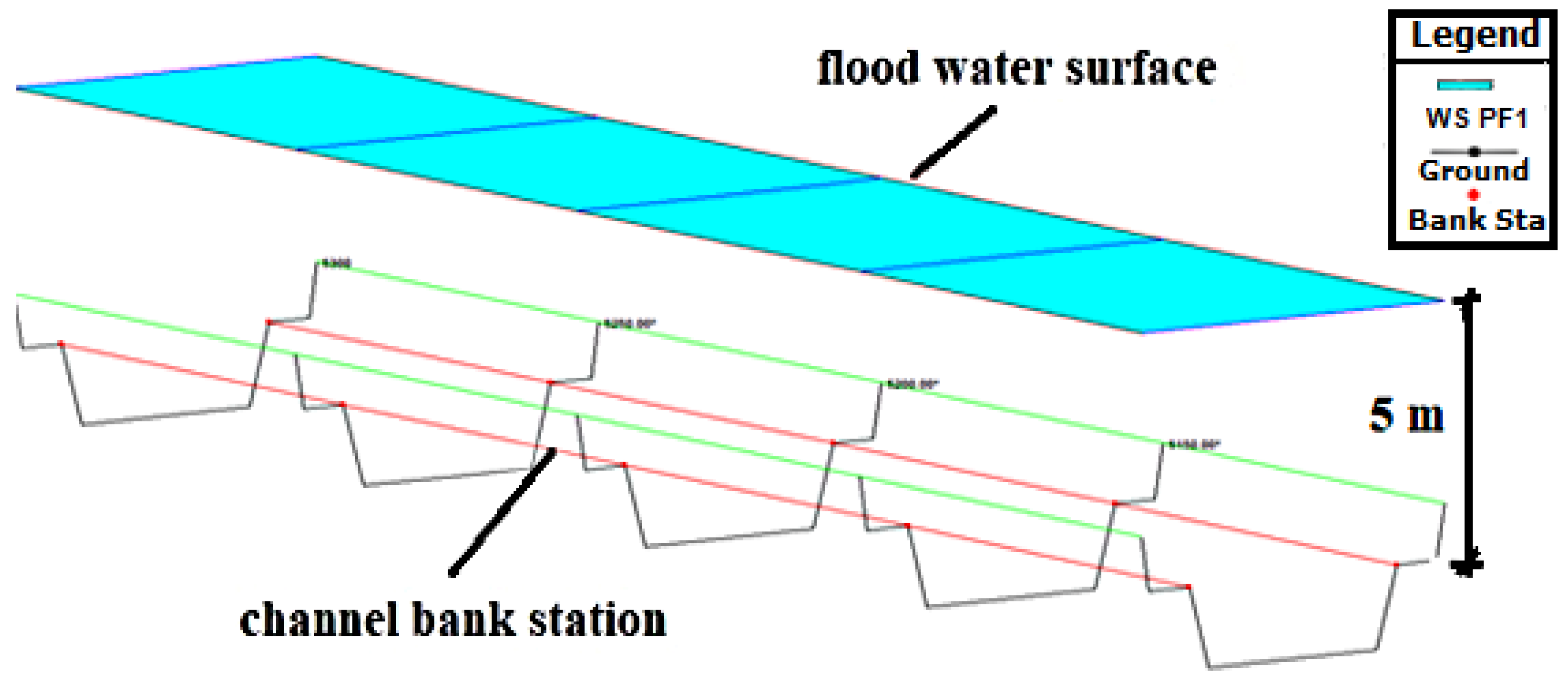
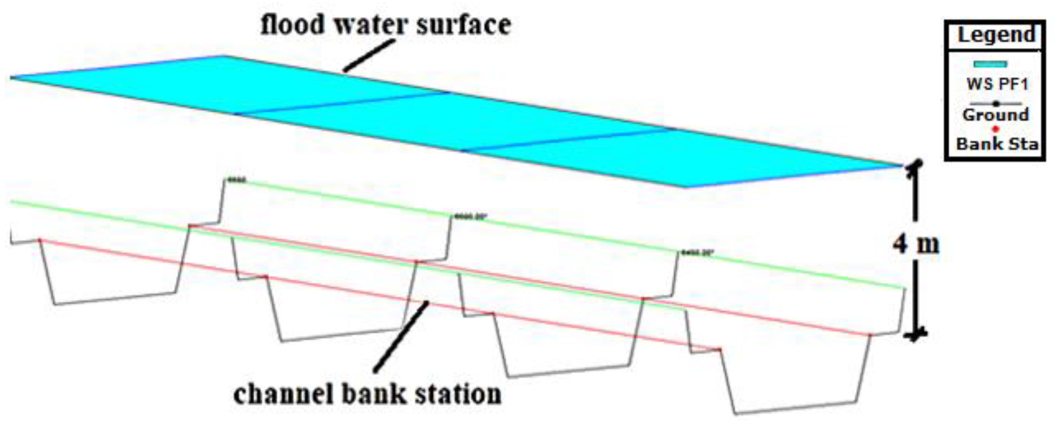
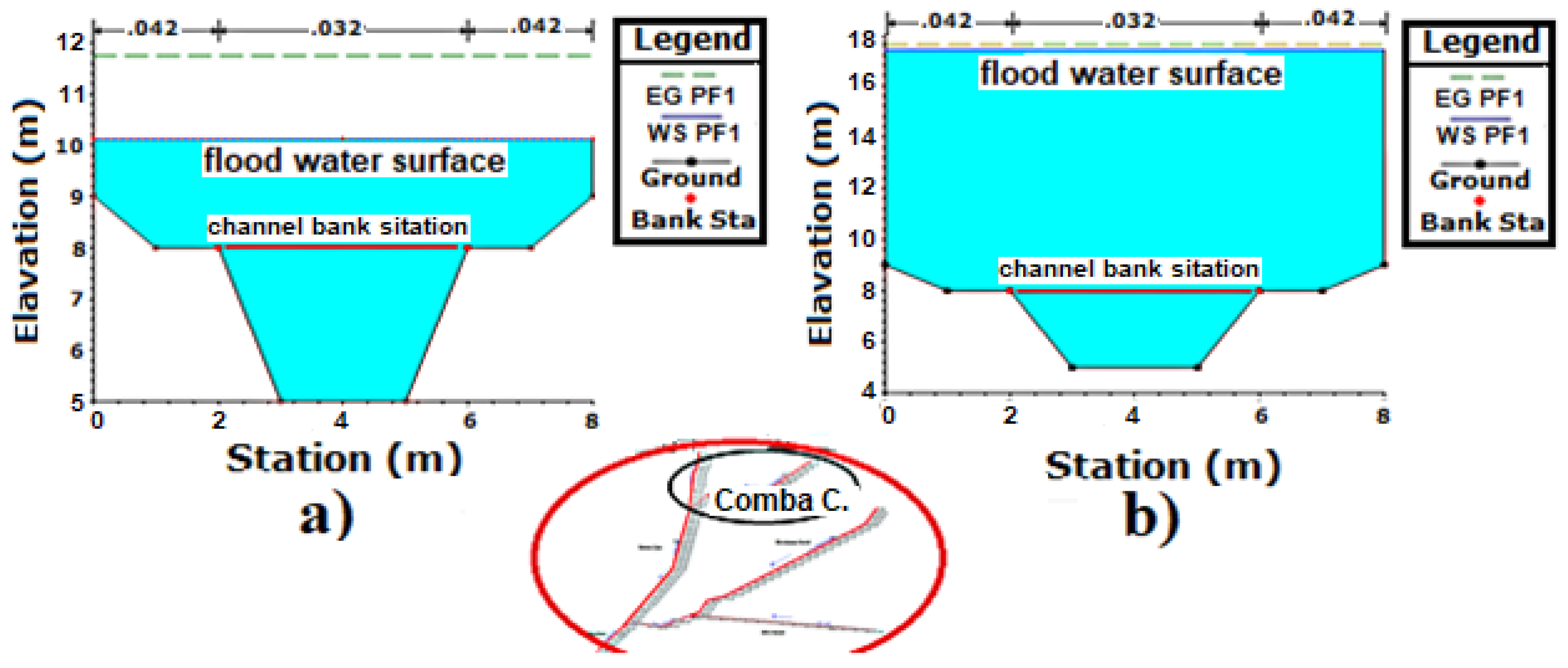
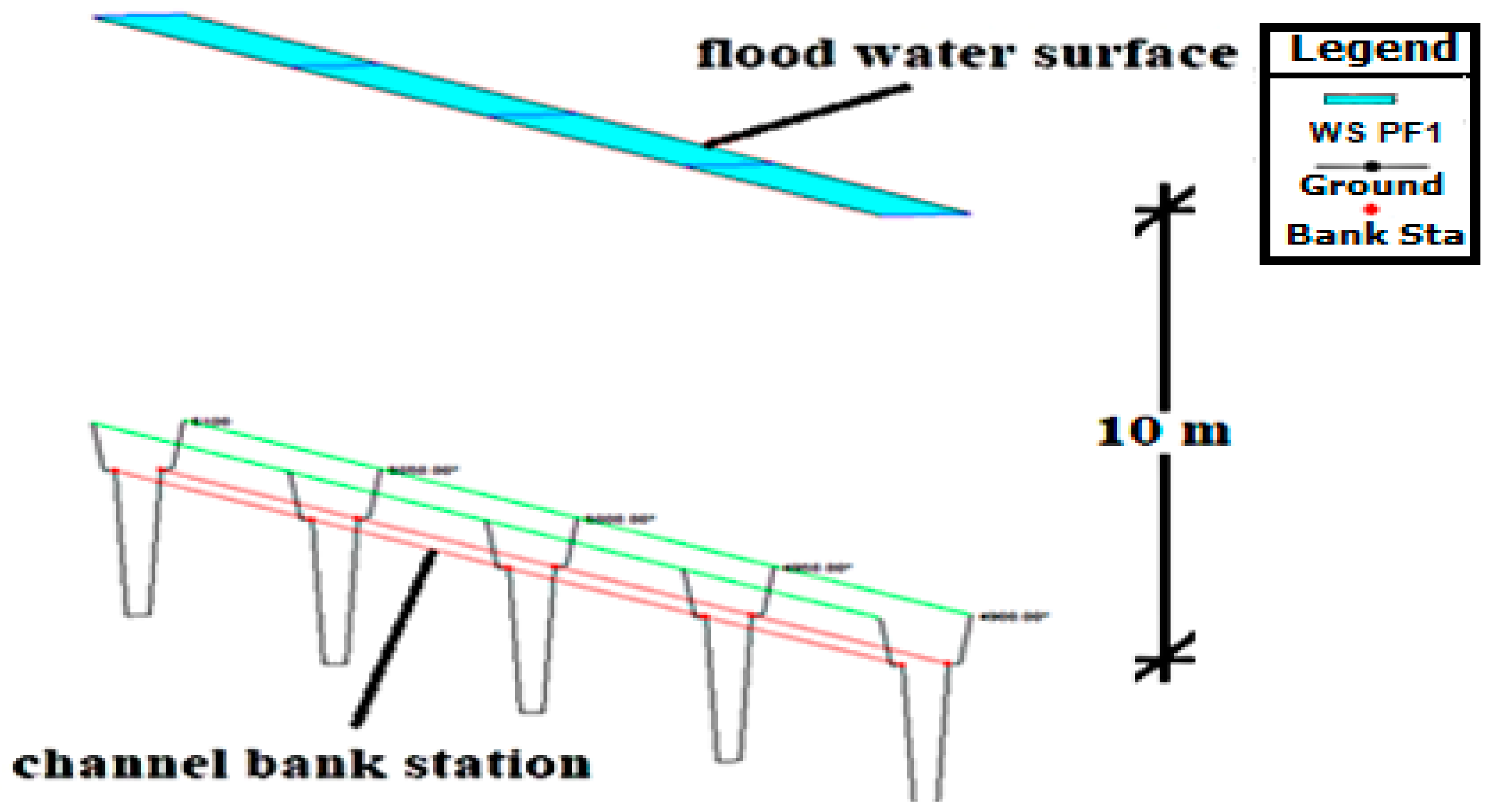
In Figure 27a,b, at discharge Q = 128 m3/s, flooding occurs about three meters above the channel top level for the Muratpaşa channel first 50 m sections, and it is about four meters above the top level of the channel for the Muratpaşa channel last sections (6550 m). Figure 28 shows perspective views of the last four sections between 6400 and 6550 m.
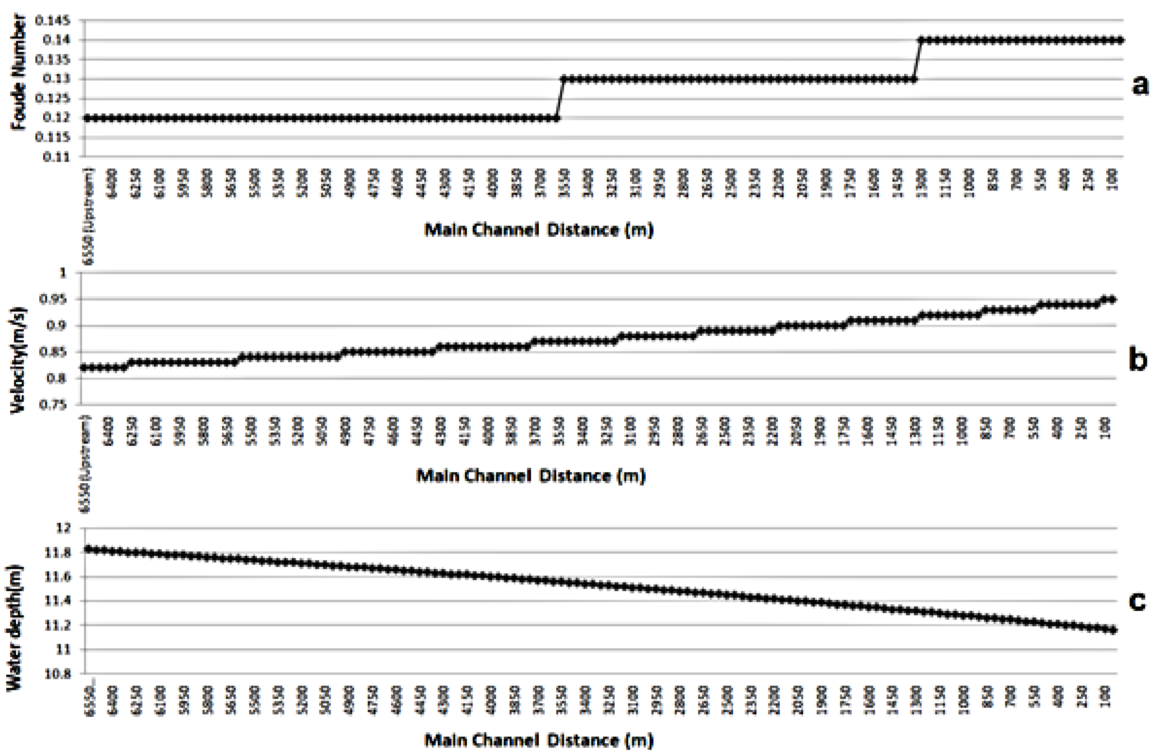
Figure 29a–c shows the changes in Froude number, velocity, and water depth along all sections in the Muratpaşa channel. When the graphs are examined, it is seen that the Froude number and the flow rate increase slowly as in the Afrin channel. This change causes an increase in water depth of about 1 m.
Figure 30a,b shows that, at discharge Q = 128 m3/s, flooding occurs two meters above the Comba channel top level for the first 50 m section, and ten meters above the channel top level for the 5100 m section. Figure 31 shows perspective views of the last five sections between 4900 and 5100 m.
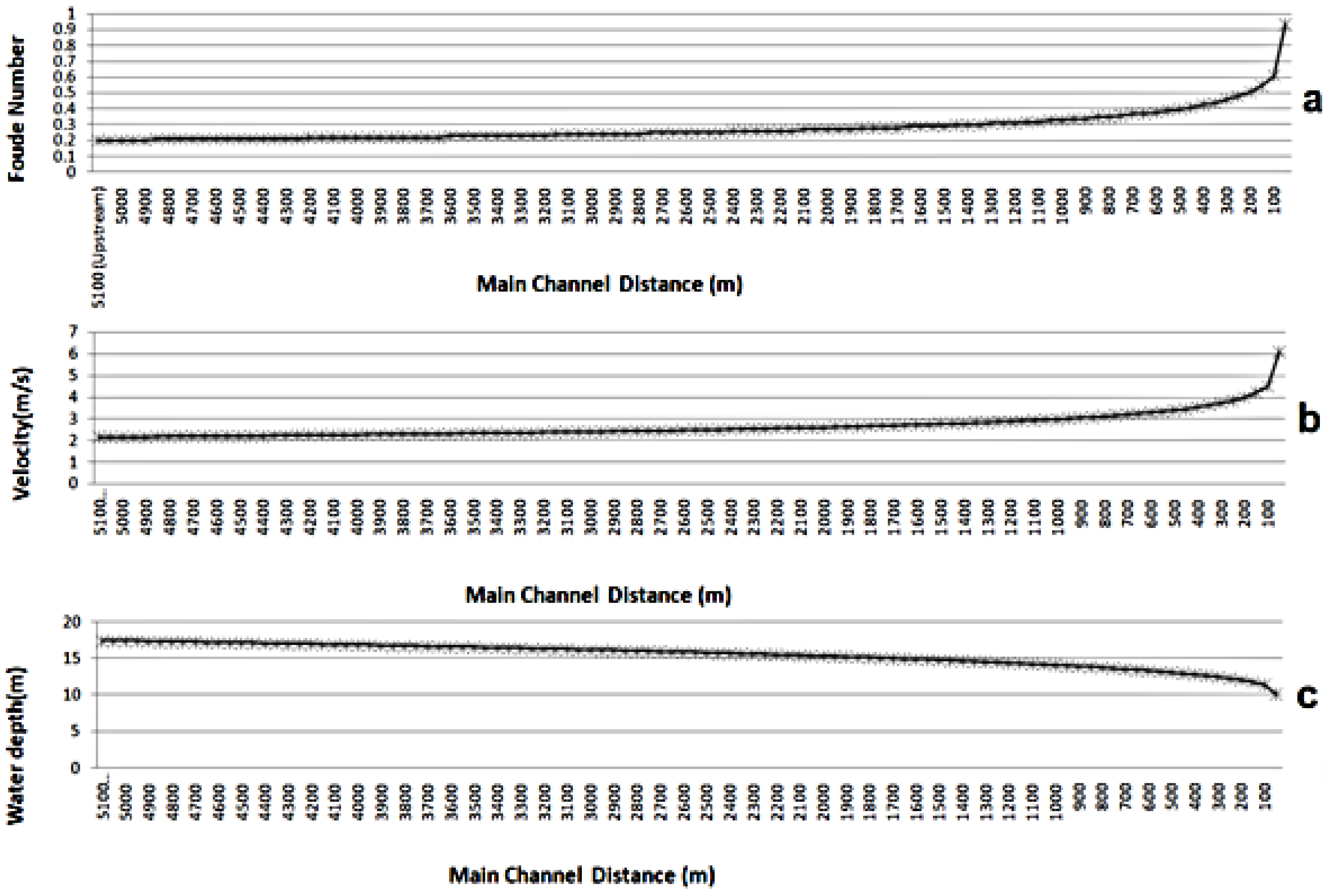
Figure 32a–c shows graphically the changes in Froude number, velocity, and water depth along all sections in the Comba channel. When the graphs are analyzed, it is seen that the Froude number increases rapidly from the upstream part with a value of 0.2 and approaches the critical value of 1.0 in the downstream part. Likewise, the velocity increases from 2 m/s and reaches 6 m/s. This rapid increase causes a change in water depth of about 7 m.
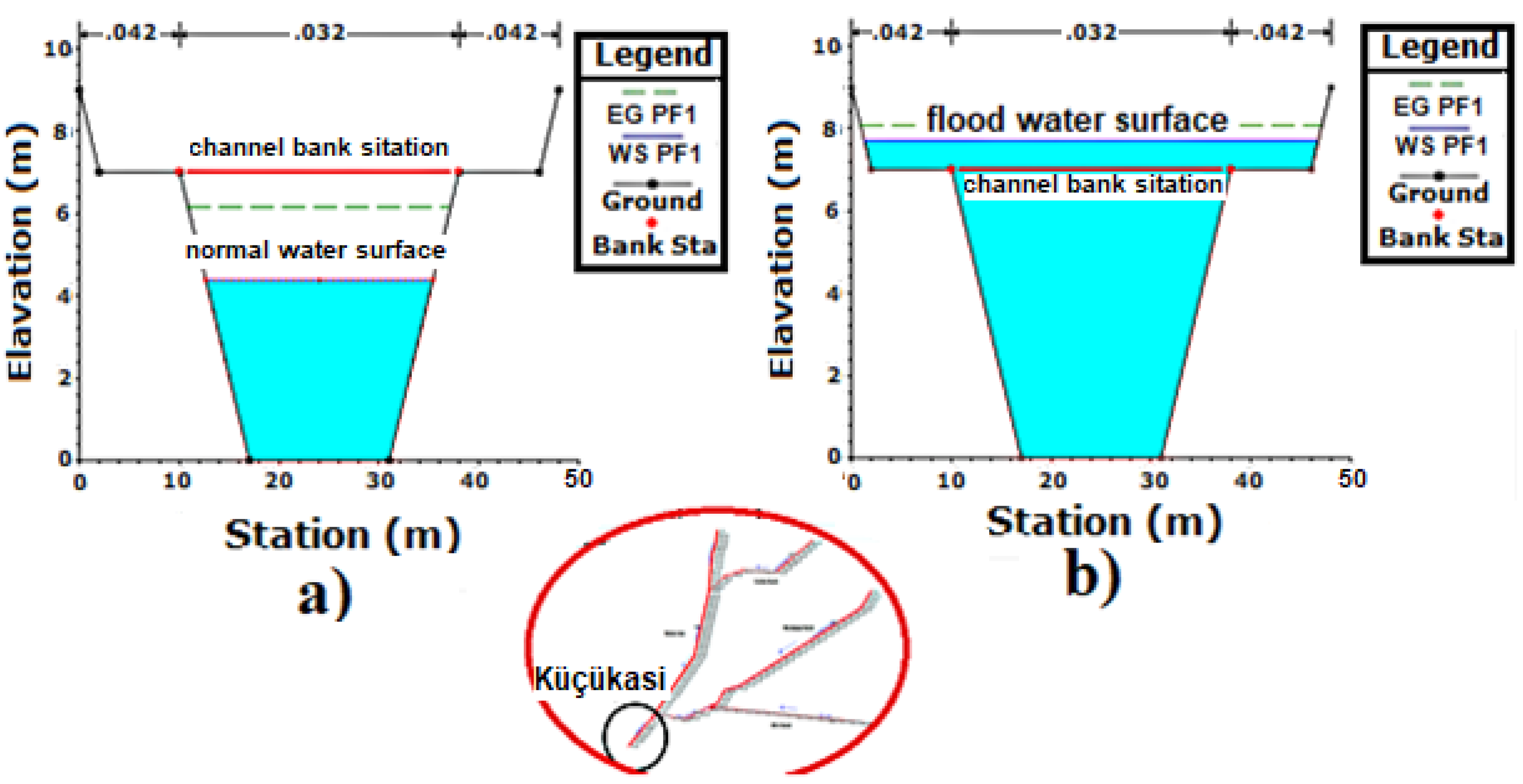
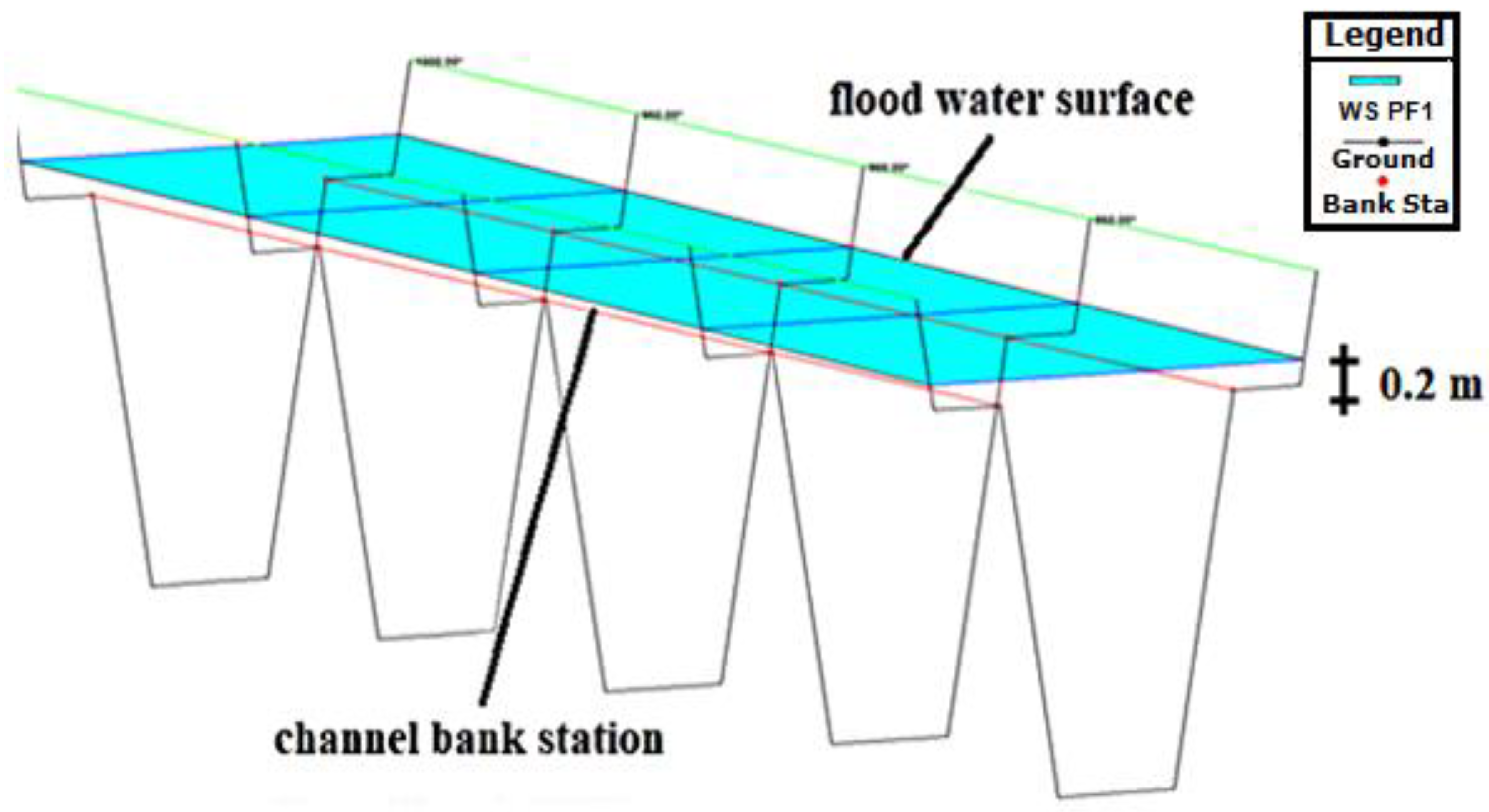
In Figure 33a,b, now at the flow rate Q = 472 m3/s, it can be observed that the first (0 m) section of the Küçükasi River was approximately 1.5 m below the top elevation of the channel, and there was no flood in this part. Flooding occurred about 0.3 m above the top level of the channel in the last 5100 m section. Figure 34 shows perspective views of the last five sections between 800 m and 1000 m.
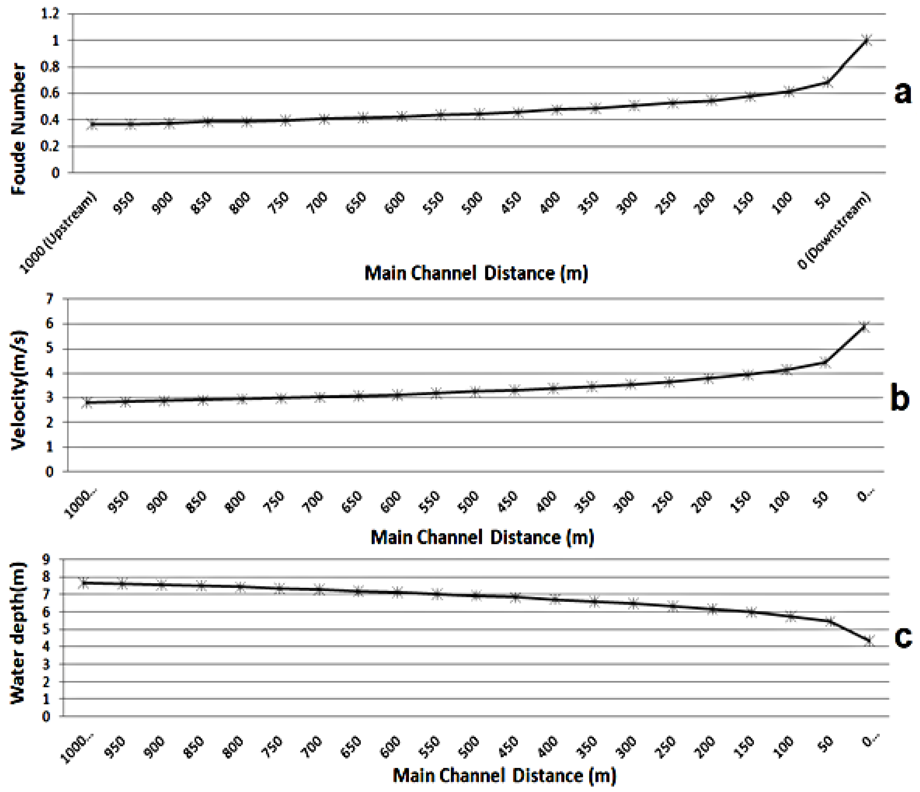
Figure 35a–c shows graphically the changes in Froude number, velocity, and water depth along all sections in the Küçükasi River. While the Froude number is about 0.3 in the upstream part, it increases rapidly and reaches the critical value 1.0 further downstream. In the same way, the velocity value rises from 2.5 m/s to 6 m/s. This increase leads to a change in water depth of about 3 m.
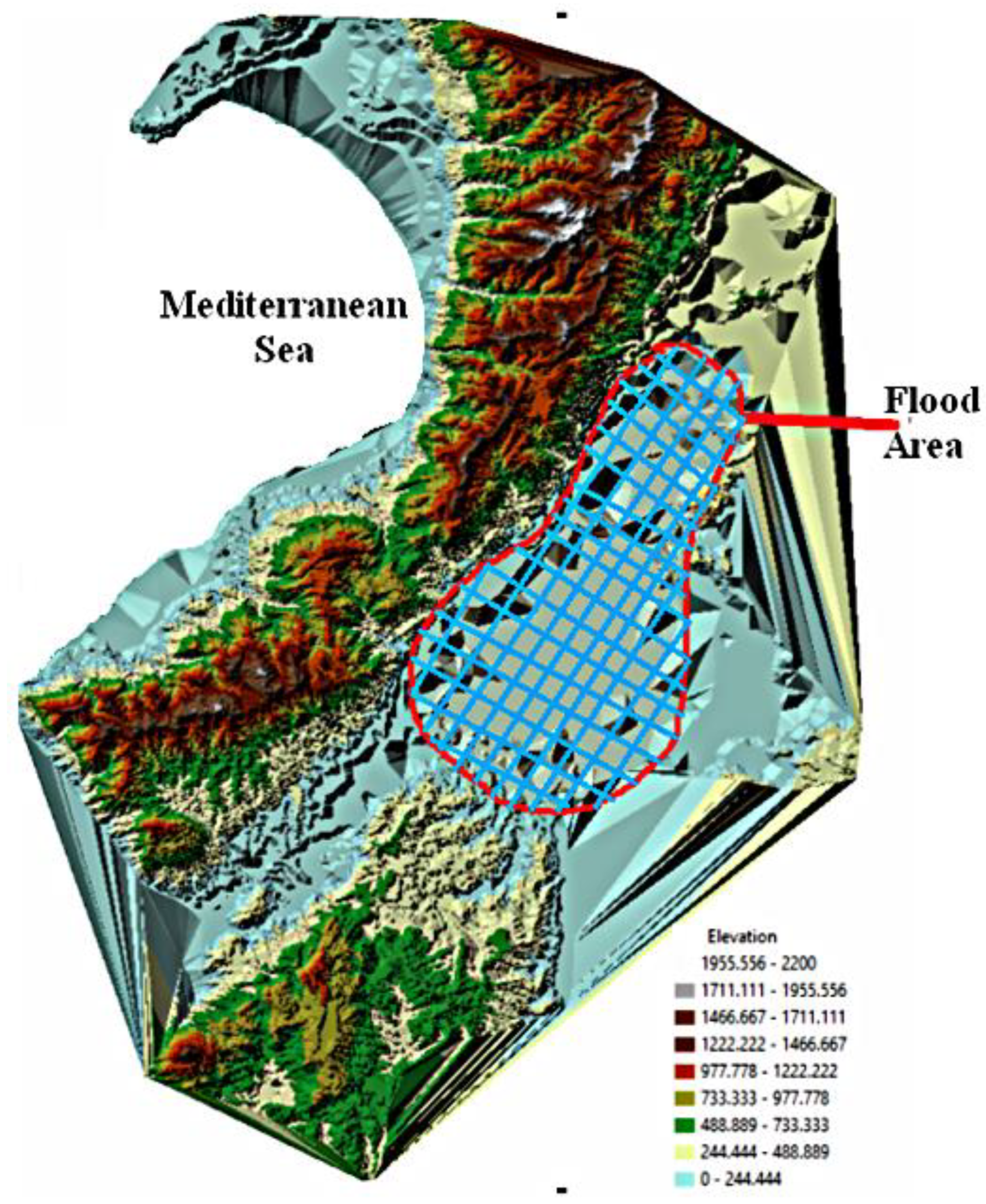
When the flood water levels found by means of the HEC-RAS program are examined, it is seen that the values are much higher than the land elevation (78 m–81 m) of the region. The digital elevation model (DEM) map relating to Hatay region is used to mark the flood area, and it is presented in Figure 36 [24].
The potential danger zone is obtained with reference to the natural elevations of the plain. According to the ESRI results, it is possible to see that a huge part of the plain including Hatay airport and agricultural areas are at risk of flooding.
4. Conclusions
Amik plain is originally a region consisting of artificially dried natural lakes and swamps under the control of local government. This area was considered as an agricultural area and improved. At an advanced stage, an airport was built in part of the plain in line with demands and research. However, in recent years, both agricultural fields and the airport have faced flooding events under climatic effects. With this study, the flood capacity of the artificial channels and the affected area was analyzed using HEC-RAS software (developed by U.S. Army Corps of Engineers Hydrologic Engineering Center-HEC).
In this case study, in order to understand the water level of Hatay’s Amik Plain during the flood, all important flow networks were examined together, and the effect of the flood was investigated. The results of the study are as follows.
By examining the hydraulic conditions of each channel and river branch, it is seen that the sections of Muratpaşa, Comba channels, and Afrin River should be increased. The presented hydraulic modeling method is sufficient to ensure flood safety, but it must be done before proposing the flood protection structure.
The highest flood value was found in the smallest channel Comba. As Hatay airport is close to this channel, necessary measures should be taken against high flood conditions in and around the airport. Considering this situation, it has been determined that it is appropriate to re-plan the Comba drainage channel.
According to the data obtained from the previous studies and model results of Amik Plain and changes in water level, it is seen that more measures should be taken during floods.
It is concluded that the capacities of measured excessive discharge values, Muratpaşa, Comba channels, and Afrin river sections are not sufficient to carry these discharge values directly to Küçükasi River.
According to the evaluation of the results obtained in this study and the similar studies presented here, the flood risk of the area is expected to increase day by day with the influence of changing climate conditions.
Depending on the changing climatic conditions, Amik Plain’s research on the relationship between precipitation and discharge will help engineers to design optimum channels that represent measures against possible floods in the future.
Author Contributions
Conceptualization, F.Ü. and B.T.; compiling data, Y.Z.K.; formal analysis, M.D.; funding acquisition, M.D.; investigation, H.V.; methodology, H.V.; project administration, M.Z.; resources, M.D.; software, Y.Z.K.; supervision, F.Ü., B.T., M.Z., and F.Ü.; validation, F.Ü.; visualization, Y.Z.K.; writing—original draft preparation, Y.Z.K. and H.V.; writing—review and editing, M.Z. All authors have read and agreed to the published version of the manuscript.
Funding
This research received no external funding.
Acknowledgments
Authors would like to thank the General Directorate for State Hydraulic Works (DSI) for sharing their measurements. This work was supported by the project of the Ministry of Education of the Slovak Republic VEGA 1/0308/20: Mitigation of hydrological hazards—floods and droughts—by exploring extreme hydroclimatic phenomena in river basins and the project of the Slovak Research and Development Agency APVV-18-0360: Active hybrid infrastructure towards a sponge city.
Conflicts of Interest
The authors declare no conflict of interest.
References
- Hazır, I.; Akgül, M.A.; Alkaya, M.; Dağdeviren, M. From 27 January to 14 March 2012 Evaluation of Floods in Amik Plain of Hatay Province Using Geographic Information Systems. In Proceedings of the 4th National Flood Symposium, Rize, Turkey, 23 November 2016. [Google Scholar]
- Turkish General Directorate of State Hydraulic Works: Preliminary Assessment of Flood Risk with Geographic Information Systems; Ankara, Turkey, 2013.
- Turkish General Directorate of State Hydraulic Works: Amik Plain Flood Report. 2012. Available online: http://www.dsi.gov.tr/docs/sempozyumlar/7-hatay-amik-ovas%C4%B1nda-meydana-gelenta%C5%9Fk%C4%B1nlar%C4%B1n-cbs-kullan%C4%B1larak-de%C4%9Ferlendirilmesi-(mda%C4%9Fdeviren)551857636298.pdf?sfvrsn=2 (accessed on 11 November 2018).
- Zelenakova, M.; Fijko, R.; Labant, S.; Weiss, E.; Markovič, G.; Weiss, R. Flood risk modelling of the Slatvinec stream in Kružlov village, Slovakia. J. Clean. Prod. 2019, 212, 109–118. [Google Scholar] [CrossRef]
- Serencam, U. Taşkın zararları ve zarar görebilirlik analizi: Trabzon Değirmendere Sanayi Mahallesi örneği. Ph.D. Thesis, Karadeniz Teknik Üniversitesi Fen Bilimleri Enstitüsü, Trabzon, Turkey, 2013. [Google Scholar]
- Kowalczuk, Z.; Świergal, M.; Wróblewski, M. River Flow Simulation Based on the HEC-RAS System. In International Conference on Diagnostics of Processes and Systems; Springer: Cham, Switzerland, 2017; p. 635. [Google Scholar] [CrossRef]
- Abd-Elhamid, H.F.; Fathy, I.; Zeleňáková, M. Flood prediction and mitigation in coastal tourism areas, a case study: Hurghada, Egypt. Nat. Hazards 2018, 93, 559–576. [Google Scholar] [CrossRef]
- Romali, N.S. Application of Hec-Ras and Arc Gis for Floodplain Mapping in Segamat Town, Malaysia. Int. J. Geomate 2018, 14, 7–13. [Google Scholar] [CrossRef]
- Ben Khalfallah, C.; Saidi, S. Spatiotemporal floodplain mapping and prediction using HEC-RAS—GIS tools: Case study of the Mejerda river, Tunisia. J. Afr. Earth Sci. 2018, 142, 44–51. [Google Scholar] [CrossRef]
- Curebal, I.; Efe, R.; Ozdemir, H.; Soykan, A.; Sönmez, S. GIS-based approach for flood analysis: Case study of Keçidere flash flood event (Turkey). Geocarto Int. 2016, 31, 355–366. [Google Scholar] [CrossRef]
- Hapciuc, O.E.; Romanescu, H.; Minea, I.; Iosub, M.; Enea, A.; Sandu, I. Flood susceptibility analysis of the cultural heritage in the Sucevita catchment (Romania). Int. J. Conserv. Sci. 2016, 7, 501–510. [Google Scholar]
- Romanescu, G.; Hapciuc, O.E.; Minea, I.; Iosub, M. Flood vulnerability assessment in the mountain–plateau transition zone: A case study of Marginea village (Romania). J. Flood Risk Manag. 2018, 11, S502–S513. [Google Scholar] [CrossRef]
- Aydin, M.C.; Yaylak, M.M. Bitlis Çayı Taşkın Hidrolojisi. Bitlis Eren Üniversitesi Fen Bilim. Derg. 2016, 5, 1. [Google Scholar] [CrossRef] [Green Version]
- Uçar, I. Flood Analysis in the Degirmendere Basin of Trabzon with the Help of Geographical Information Systems and a Hydraulic Model; Gazi University: Ankara, Turkey, 2010. [Google Scholar]
- Özdemir, H. HEC-GeoRAS and HEC-RAS for Mapping Floods: Havran Stream Sample (Balıkesir). In Proceedings of the Map and Cadastre Engineers National Geographic Information Systems Congress, Trabzon, Turkey, 30 October–11 November 2007. [Google Scholar]
- Singh, V.P.; Fiorentino, M. Geographical Information Systems in Hydrology; Kluwer Academic Publishers: London, UK, 1996; ISBN 9780792342267. [Google Scholar]
- Turkish General Directorate of State Hydraulic Works: Flood Hydrology Design Guide; Ankara, Turkey, 2012.
- Bedient, P.B.; Wayne, C.H.; Vieux, B.E. Hydrology and Floodplain Analysis | Pearson; Pearson: London, UK, 2008; ISBN 9780131745896. [Google Scholar]
- Dyhouse, G.; Hachett, J.; Benn, J. Floodplain Modeling Using HECRAS; Haestad Press: Waterbury, CT, USA, 2003; ISBN 0971414106. [Google Scholar]
- Maidment, D.R. Djokic Hydrologic and Hydraulic Modeling Support: With Geographic Information Systems; ESRI Press: Redlands, CA, USA, 2000; ISBN 9781879102804. [Google Scholar]
- USACE HEC-RAS River Analysis System, User’s Manual; US Army Corps of Engineers: Davis, CA, USA, 2016.
- Chow, V.T. Open-Channel Hydraulics; McGraw-Hill: New York, NY, USA, 1959; pp. 19–148. [Google Scholar]
- Map Showing Location of Hatay Airport. Available online: earth.google.com/web/ (accessed on 20 July 2020).
- ESRI Inc. ArcGIS 10.6; ESRI Inc.: Redlands, CA, USA, 2018. [Google Scholar]
Figure 1.
Plain location and the lake area before it was dried [1].
Figure 1.
Plain location and the lake area before it was dried [1].

Figure 2.
Schematic representation of Asi and Küçükasi Rivers, drainage canals, and current observation stations [1,3].


Figure 5.
Flood photos of flood in 2012 [1,3]. (a) General view of Amik Plain; (b) Hatay airport during the flood 2012; (c) Specific view of Hatay airport during the flood 2012.

Figure 6.
General view of Amik Plain after rainfall in 2019.

Figure 7.
Flow chart showing the methodology adopted.

Figure 8.
Representation of quantities in energy equations [21].
Figure 8.
Representation of quantities in energy equations [21].

Figure 9.
Definitions of subsections of HEC-RAS [21].
Figure 9.
Definitions of subsections of HEC-RAS [21].

Figure 10.
Quantities in the momentum method [21].
Figure 10.
Quantities in the momentum method [21].

Figure 11.
HEC-RAS main button bar [21].
Figure 11.
HEC-RAS main button bar [21].

Figure 12.
Screenshot of Hatay Airport from Google Earth [24].
Figure 12.
Screenshot of Hatay Airport from Google Earth [24].

Figure 13.
Flood model created in HEC-RAS program.

Figure 14.
Sections created in the HEC-RAS program: (a) Küçükasi river; (b) Karasu river1; (c) Karasu River 2; (d) Comba channel; (e) Muratpaşa channel; (f) Afrin channel1; and (g) Afrin channel 2.
Figure 14.
Sections created in the HEC-RAS program: (a) Küçükasi river; (b) Karasu river1; (c) Karasu River 2; (d) Comba channel; (e) Muratpaşa channel; (f) Afrin channel1; and (g) Afrin channel 2.

Figure 15.
Processing of flood flows into the HEC-RAS program.

Figure 16.
(a) Karasu River second part and Q = 216 m3/s discharge for the first (50 m) section; (b) Karasu River second part and Q = 216 m3/s discharge for the last 2750 m; (c) first perspective view for all sections; (d) second perspective view for all sections.
Figure 16.
(a) Karasu River second part and Q = 216 m3/s discharge for the first (50 m) section; (b) Karasu River second part and Q = 216 m3/s discharge for the last 2750 m; (c) first perspective view for all sections; (d) second perspective view for all sections.

Figure 17.
(a) Graph of Froude number change across all sections for the Karasu river second part where Q = 216 m3/s; (b) velocity change graph; (c) water depth change graph.
Figure 17.
(a) Graph of Froude number change across all sections for the Karasu river second part where Q = 216 m3/s; (b) velocity change graph; (c) water depth change graph.

Figure 18.
(a) Karasu River first part and discharge Q = 216 m3/s for the first (50 m) section; (b) Karasu River first part and discharge Q = 216 m3/s for the last (5250 m) section.
Figure 18.
(a) Karasu River first part and discharge Q = 216 m3/s for the first (50 m) section; (b) Karasu River first part and discharge Q = 216 m3/s for the last (5250 m) section.

Figure 19.
Perspective view for sections 5100–5250 m for discharge Q = 216 m3/s in the Karasu River first part.
Figure 19.
Perspective view for sections 5100–5250 m for discharge Q = 216 m3/s in the Karasu River first part.

Figure 20.
(a) When the discharge is Q = 216 m3/s, the Froude number changes across all sections for the first part of Karasu River; (b) velocity change graph; (c) water depth change graph.
Figure 20.
(a) When the discharge is Q = 216 m3/s, the Froude number changes across all sections for the first part of Karasu River; (b) velocity change graph; (c) water depth change graph.

Figure 21.
(a) Cross-section of the first 50 m of the Afrin Channel and (b) cross-section of the last 1250m of the Afrin Channel, both at discharge Q = 256 m3/s.
Figure 21.
(a) Cross-section of the first 50 m of the Afrin Channel and (b) cross-section of the last 1250m of the Afrin Channel, both at discharge Q = 256 m3/s.

Figure 22.
Afrin channel part one: perspective view for all sections.

Figure 23.
(a) Froude number change graph across all sections for the Afrin channel first part when Q = 256 m3/s; (b) velocity change graph; (c) water depth graph.
Figure 23.
(a) Froude number change graph across all sections for the Afrin channel first part when Q = 256 m3/s; (b) velocity change graph; (c) water depth graph.

Figure 24.
(a) Afrin channel second part, section view for the first 100 m; (b) Afrin channel second part, section view for the last 5300 m, both at discharge Q = 256 m3/s.
Figure 24.
(a) Afrin channel second part, section view for the first 100 m; (b) Afrin channel second part, section view for the last 5300 m, both at discharge Q = 256 m3/s.

Figure 25.
Perspective view for sections 5100–5300 m at discharge Q = 256 m3/s in the Afrin channel second part.
Figure 25.
Perspective view for sections 5100–5300 m at discharge Q = 256 m3/s in the Afrin channel second part.

Figure 26.
(a) Froude number change graph for all sections of the second part of the Afrin channel when Q = 256 m3/s; (b) velocity change graph; (c) water depth change graph.
Figure 26.
(a) Froude number change graph for all sections of the second part of the Afrin channel when Q = 256 m3/s; (b) velocity change graph; (c) water depth change graph.

Figure 27.
(a) The first (50 m) cross-section in the Muratpaşa channel; (b) the last (6550 m) crosssection in the Muratpaşa channel, both at flow rate Q = 128 m3/s.
Figure 27.
(a) The first (50 m) cross-section in the Muratpaşa channel; (b) the last (6550 m) crosssection in the Muratpaşa channel, both at flow rate Q = 128 m3/s.

Figure 28.
Perspective view for sections 6400–6550 m at discharge Q = 128 m3/s in the Muratpaşa channel.
Figure 28.
Perspective view for sections 6400–6550 m at discharge Q = 128 m3/s in the Muratpaşa channel.

Figure 29.
(a) Froude number change graph across all sections at discharge Q = 128 m3/s in Muratpaşa channel; (b) velocity change graph; (c) water depth change graph.
Figure 29.
(a) Froude number change graph across all sections at discharge Q = 128 m3/s in Muratpaşa channel; (b) velocity change graph; (c) water depth change graph.

Figure 30.
(a) Cross-sectional view of Comba channel first 50 m; (b) cross-sectional view of Comba channel last 5100 m, both at discharge Q = 128 m3/s.
Figure 30.
(a) Cross-sectional view of Comba channel first 50 m; (b) cross-sectional view of Comba channel last 5100 m, both at discharge Q = 128 m3/s.

Figure 31.
Perspective view for sections 6400–6550 m in Comba channel at discharge Q = 128 m3/s.

Figure 32.
(a) Froude number change graph across all sections in Comba channel at discharge Q = 128 m3/s; (b) velocity change graph; (c) water depth change graph.
Figure 32.
(a) Froude number change graph across all sections in Comba channel at discharge Q = 128 m3/s; (b) velocity change graph; (c) water depth change graph.

Figure 33.
(a) First (0 m) cross-section in Küçükasi River; (b) last (1000 m) cross-section in Küçükasi river, both at discharge Q = 472 m3/s.
Figure 33.
(a) First (0 m) cross-section in Küçükasi River; (b) last (1000 m) cross-section in Küçükasi river, both at discharge Q = 472 m3/s.

Figure 34.
Perspective view for sections between 800 m and 1000 m in Küçükasi river at discharge Q = 472 m3/s.
Figure 34.
Perspective view for sections between 800 m and 1000 m in Küçükasi river at discharge Q = 472 m3/s.

Figure 35.
(a) Froude number change graph for the Küçükasi river at the discharge Q = 472 m3/s; (b) velocity change graph; (c) water depth change graph.
Figure 35.
(a) Froude number change graph for the Küçükasi river at the discharge Q = 472 m3/s; (b) velocity change graph; (c) water depth change graph.

Figure 36.
Marked flood area using digital elevation 3D model map of Hatay [24].
Figure 36.
Marked flood area using digital elevation 3D model map of Hatay [24].


Table 1.
Subcritical current contraction and expansion coefficients.
| Transition Type | Contraction | Expansion |
|---|---|---|
| No Transition Loss | 0 | 0 |
| Smooth Transition | 0.1 | 0.3 |
| Bridge Transition | 0.3 | 0.5 |
| Sudden Transition | 0.6 | 0.8 |
Table 2.
Values for different types of channels [22].
Table 2.
Values for different types of channels [22].
| Type of Channel and Description | Minimum | Normal | Maximum |
|---|---|---|---|
| Natural streams-minor streams (top width at floodstage < 100 ft) | |||
| 1. Main Channels | |||
| a. clean, straight, full stage, no rifts or deep pools | 0.025 | 0.030 | 0.033 |
| b. same as above, but more stones and weeds | 0.030 | 0.035 | 0.040 |
| c. Clean, winding, some pools and shoals | 0.033 | 0.040 | 0.045 |
| d. same as above, but some weeds and stones | 0.035 | 0.045 | 0.050 |
| e. same as above, lower stages, more ineffective slopes and sections | 0.040 | 0.048 | 0.055 |
| f. same as "d" with more stones | 0.045 | 0.050 | 0.060 |
| g. sluggish reaches, weedy, deep pools | 0.050 | 0.070 | 0.080 |
| h. very weedy reaches, deep pools, or noodways with heavy stand of timber and underbrush | 0.075 | 0.100 | 0.150 |
| 2. Mountain streams, no vegetation in channel, banks usually steep, trees and brush along banks submerged at high stages | |||
| a. bottom: gravels, cobbles, and lew boulders | 0.030 | 0.040 | 0.050 |
| b. bottom: cobbles with large boulders | 0.040 | 0.050 | 0.070 |
| 3. Floodplains | |||
| a. Pasture, no brush | |||
| 1. short grass | 0.025 | 0.030 | 0.035 |
| 2. high grass | 0.030 | 0.035 | 0.050 |
| b. Cultivated areas | |||
| 1. no crop | 0.020 | 0.030 | 0.040 |
| 2. mature row crops | 0.025 | 0.035 | 0.045 |
| 3. mature field crops | 0.030 | 0.040 | 0.050 |
| c. Brush | |||
| 1. scattered brush, heavy weeds | 0.035 | 0.050 | 0.070 |
| 2. light brush and trees, [n winter | 0.035 | 0.050 | 0.060 |
| 3. light brush and trees, in summer | 0.040 | 0.060 | 0.080 |
| 4. medium to dense brush, in winter | 0.045 | 0.070 | 0.110 |
| 5. medium to dense brush, in summer | 0.070 | 0.100 | 0.160 |
| d. Trees | |||
| 1. dense willows, summer, straight | 0.110 | 0.150 | 0.200 |
© 2020 by the authors. Licensee MDPI, Basel, Switzerland. This article is an open access article distributed under the terms and conditions of the Creative Commons Attribution (CC BY) license (http://creativecommons.org/licenses/by/4.0/).
Share and Cite
MDPI and ACS Style
Üneş, F.; Ziya Kaya, Y.; Varçin, H.; Demirci, M.; Taşar, B.; Zelenakova, M. Flood Hydraulic Analyses: A Case Study of Amik Plain, Turkey. Water 2020, 12, 2070. https://0-doi-org.brum.beds.ac.uk/10.3390/w12072070
AMA Style
Üneş F, Ziya Kaya Y, Varçin H, Demirci M, Taşar B, Zelenakova M. Flood Hydraulic Analyses: A Case Study of Amik Plain, Turkey. Water. 2020; 12(7):2070. https://0-doi-org.brum.beds.ac.uk/10.3390/w12072070
Chicago/Turabian StyleÜneş, Fatih, Yunus Ziya Kaya, Hakan Varçin, Mustafa Demirci, Bestami Taşar, and Martina Zelenakova. 2020. "Flood Hydraulic Analyses: A Case Study of Amik Plain, Turkey" Water 12, no. 7: 2070. https://0-doi-org.brum.beds.ac.uk/10.3390/w12072070
Note that from the first issue of 2016, this journal uses article numbers instead of page numbers. See further details here.