An Empirical Study on the Ecological Economy of the Huai River in China


1
School of Urban and Environmental Science, Huaiyin Normal University, Huai’an 223300, China
2
Urban Design Analysis Lab, Graduate School of Urban Studies, Hanyang University, Seoul 04763, Korea
*
Authors to whom correspondence should be addressed.
Water 2020, 12(8), 2162; https://0-doi-org.brum.beds.ac.uk/10.3390/w12082162
Submission received: 8 June 2020
/
Revised: 25 July 2020
/
Accepted: 29 July 2020
/
Published: 31 July 2020
(This article belongs to the Special Issue Management and Monitoring of Urban and Rural Ecological Water Resources)
Abstract
:The Huai River is an important flood control and discharge river in the middle and east of China, and the development of ecological economy with regional advantages is significant for the protection and improvement of the resources and environment of the basin. On the basis of defining the connotation of an ecological economic system, this study constructed an index system, and it applied the methods of data envelopment analysis (DEA) and exploratory spatial data analysis (ESDA) to study the ecological economy of the Huai River. This study concluded that (1) the efficiency in most areas was efficient, but inefficient in a few areas; (2) the causes of inefficiency were unreasonable production scale and unqualified production technology, which led to redundant input of resources, insufficient output of days with good air quality, and excessive output of particulate matter with less than or equal to 2.5 microns in diameter (PM2.5); and (3) the efficiency was different in different regions, so it was necessary to respectively formulate and implement strategies for protection and development of resources and environment. The research results can be used as an important reference for formulating ecological economic policies around the world.

1. Introduction
The resource depletion and environmental pollution [1,2,3,4,5] caused by the rapid development of modern society and economy are becoming more and more serious and have been identified as global public health issues [6]. Water, the basis of all life and an indispensable and irreplaceable element of natural resources and environment for social and economic development, is often not accessible for approximately 11% of the world’s population [7]. The global extraction of raw materials has increased from about 23 billion tons to more than 80 billion tons since 1970 [8], and CO2 concentration in the global atmosphere has increased from about 325 ppm to more than 410 ppm in this same period [9]. Heavy haze pollution, which mainly comprises PM2.5 with serious exceedance, causes 12–16 thousand premature deaths every year in China, the world’s second largest economy [5].
The Huai River Basin is a highly polluted river basin in China due to the traditional rapid economic growth [1]. Several serious pollution incidents occurred in this area, which risked the life safety of millions of people living alongside the rivers. For a long time, many scholars have paid attention to the problems of rainfall, flood disaster [10], water resource consumption [2], and water resource pollution [1] in the Huai River Basin, and there is a lack of research on the transformation of economic growth mode in the basin.
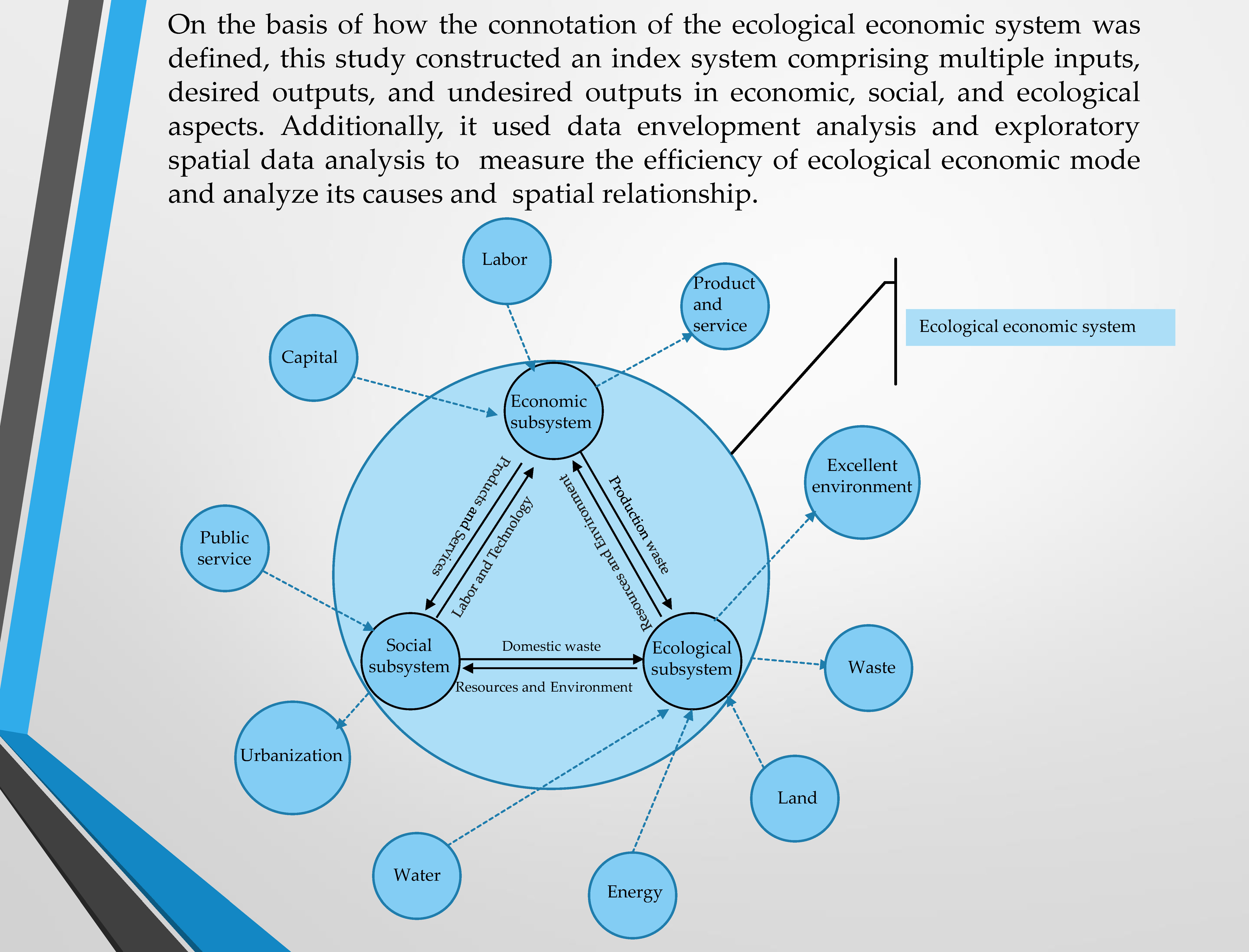
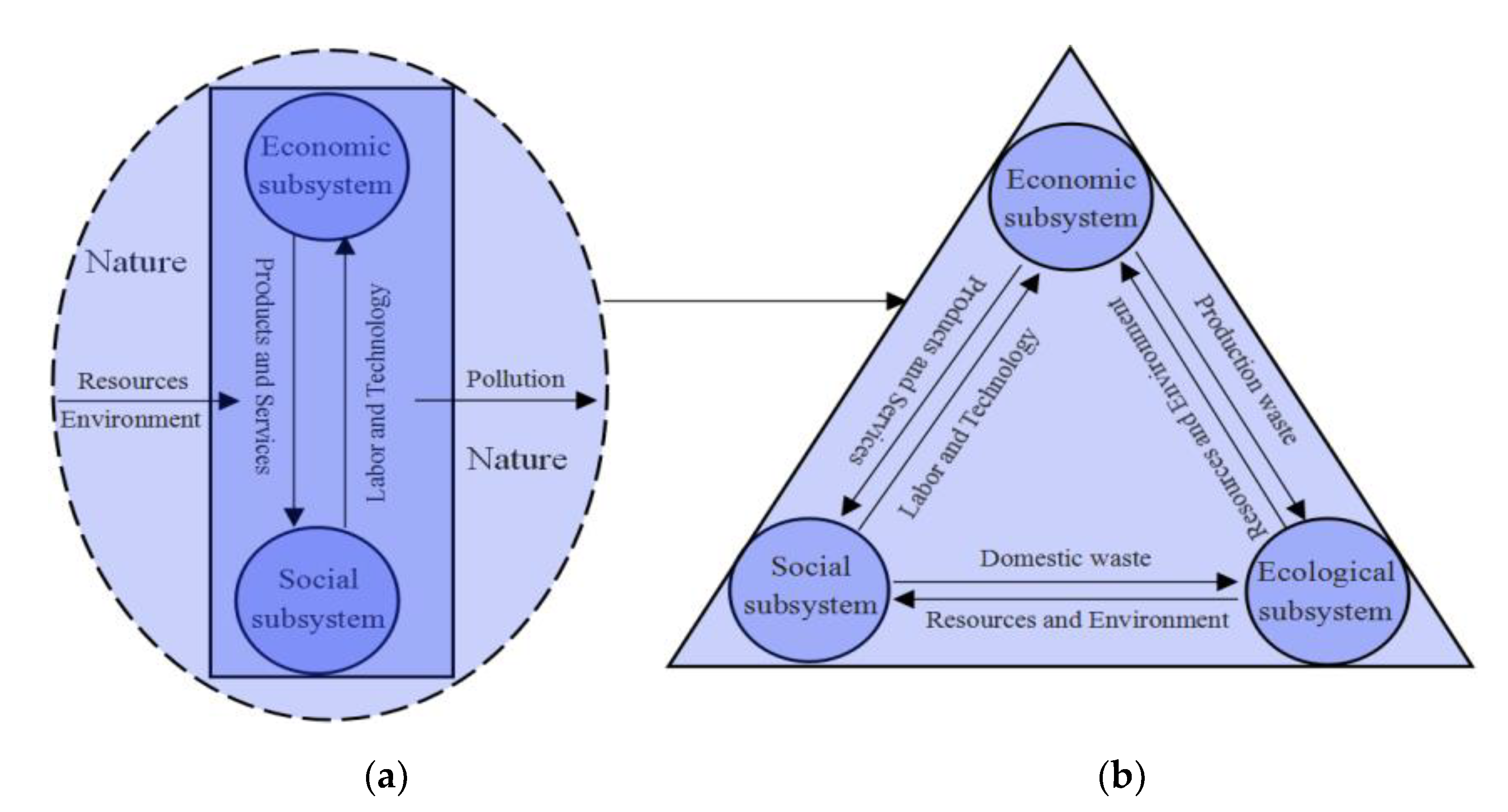
People have gradually realized that the conventional economic growth model (Figure 1a), which isolates humans from nature, while indiscriminately exploiting natural resources, has generated severe resource crunch and exerted considerable environmental pressure on world development [11]. Just as pointed out in the program “The Economics of Ecosystems and Biodiversity” (TEEB) commissioned by the G8 + 5 group of nations, living organisms and the non-living environment in nature provide services such as resource supply, environmental regulation, habitat, and cultural facilities, which have important use value and non-use value for the development of human society, but their integrity, health, and resilience are critical thresholds for the service provision. When resources are depleted or the environment is degraded, high follow-up costs of the loss of natural services become manifest especially in health effects, production losses, and costs for cleaning and restoration. From the perspective of economics, nature represents a form of capital whose dividend is paid in the form of nature services [12,13,14,15]. Therefore, the ecological economic mode (Figure 1b), which considers nature to be an integral part of the human system, is expected to become the most effective way to solve the contradiction between social economic development and ecological security [5]. The essence of the eco-economic mode is to develop society and economy on the basis of the ecological environment by the establishment of a compound ecosystem consisting of economy, society, and nature with a virtuous cycle, so as to achieve the “win–win” of economic development and ecological protection. The Venn diagram [16] representing an ecological economic system comprises three basic subsystems: the economy, society, and ecology (Figure 1b). The economic subsystem receives labor and technology inputs from the social subsystem and outputs products and services into the social subsystem. The social subsystem receives environmental resources from the ecological subsystem and outputs domestic waste into the ecological subsystem. The ecological subsystem receives production waste from the economic subsystem and outputs resources and environments into the economic subsystem. These three subsystems form a complex ecological economic system through the interweaving of material circulation and energy transfer.
How to speed up the development of social economy and maintain the virtuous cycle of ecological economic system? Developing an ecological economy and improving its efficiency can achieve the above two goals at the same time. The efficiency of eco-economy refers to the utilization degree of various resources and the discharge degree of waste in the eco-economic mode. It reflects the ability to produce more goods and services, consume less resources, and have less impact on the environment. Therefore, we should scientifically evaluate the efficiency of eco-economic mode and explore its causes and spatial characteristics, so as to provide a factual basis for the regional accurate formulation and implementation of resources and environment protection and development planning and policies.
2. Literature Review
Ecological economic efficiency can be measured by examining the relationship between human production activities and regional ecological capacity [17]. The concept of ecological economic efficiency was first proposed by Schaltegger and Sturm in 1990 [18] and was further developed by the World Business Council for Sustainable Development in 1992 [19]. Since then, an increasing number of scholars have conducted research on ecological economic efficiency. Its definition focuses on the relationship between the economy, society, and ecology, wherein economic outputs meet the demands of people, resource consumption and environmental pollution are controlled, and ecology and the economy present coordinated development.
Composite index and data envelopment analysis (DEA) are the most commonly used methods for measuring regional ecological economic efficiency. A composite index involves constructing an index system from a composite perspective; different studies have used the ratio method [20], grey relational analysis [21], analytic hierarchy process [22], and Shannon entropy [23] for measurement. DEA involves constructing an index system from the perspective of inputs and outputs and uses the DEA method [11,24,25] for measurement. Both methods can effectively evaluate regional ecological economic efficiency. The composite index method is simple to use and comprehensive in its consideration of factors, but data distortion occurs easily because of dimensionless processing. Moreover, because the index system is not developed in accordance with the law of production function, it only measures the levels of but not the relationship between inputs and outputs. However, because the DEA method does not require the dimensionless processing of variables, it can maximize the integrity of original information. In addition, it can measure the conversion degree between inputs and outputs and achieve the optimal improved value, which can provide management departments with a scientific basis for policy-making.
In recent years, the DEA model has been widely used in academia; it has been continuously improved to meet the requirements for measuring ecological economic efficiency in different situations (Table 1). The basic form of the DEA model is the Charnes–Cooper–Rhodes (CCR) model [26]. The DEA model was improved to the Banker–Charnes–Cooper (BCC) [27] and slacks-based measure (SBM) [28] models on the basis of the CCR model. The comprehensive ecological economic efficiency [29] of the decision-making units can be measured by constructing multiple input indicators and output indicators in the CCR model under the assumption that the cone condition is satisfied. The BCC model measures the technical efficiency of the ecological economics of decision-making units under the assumption that the cone and convexity conditions are satisfied [27]. The SBM model improves the measurement accuracy of the ecological economic efficiency of decision-making units by constructing multiple input indicators and desired and undesired output indicators and directly adding slack variables to the objective function [28,30]. Thereafter, super-efficiency DEA models (the S-CCR model [24] S-SBM model [31]) for improving the accuracy and discrimination of ecological economic efficiency, cross-efficiency DEA models (the C-SBM model [32]), and network-efficiency DEA models that consider the input–output immediate process (the N-SBM model [25]) were constructed separately to measure ecological economic efficiency more objectively and comprehensively.
The appropriate DEA model was chosen by scholars to evaluate the efficiency of ecological economy in various fields. Rybaczewska-Błażejowska and Gierulski [27] built a BCC-DEA model in which a set of impact categories from the life cycle assessment (LCIA) stage were used as input values and economic indicator was used as a output value to evaluate efficiencies of agricultural ecological technology about 28 EU countries. Wang et al. [28] created an SBM-DEA model with a set of indicators including input and desired output and undesired output to assess the industrial ecological efficiency of nine cities in Fujian Province, in the model the input index set was made up of the consumption of standard coal and the consumption of fresh water, and the desired output index set was made up of industrial added value, and the undesired output index set was made up of the discharge amount of industrial wastewater and the emission amount of industrial waste gas. Hao et al. [24] took total water diversion and air pollutant emission from fixed sources as input indicators, and took GDP per capita, afforestation, non-poverty rate as output indicators, and then used Super-CCR model to evaluate ecological efficiency in order to evaluate the effect of Kyrgyzstan’s ecological policy and government governance. Yu et al. [31] selected labor, capital, and energy as input, and selected GDP as ideal output and CO2 emissions as bad output to investigate the regional heterogeneity of China’s energy efficiency under the “new normal”, using the method of Super-SBM model. lo Storto [32] constructed a set of indicators including input indicators, desired output indicators, and undesired output indicators to evaluate and rank the ecological efficiency of Italian capital cities with the cross-efficiency SBM model. Kiani Mavi et al. [25] built a network SBM-DEA model with a public weight considering intermediate products and bad output to evaluate and rank the comprehensive efficiency of the Organization for Economic Cooperation and Development (OECD) countries including ecological efficiency and ecological innovation.
Results of related research on the construction of index system and evaluation methods of ecological economic efficiency measurement were very valuable. The index system included all aspects and links of input and output, and the evaluation methods included the CCR-DEA model to measure the comprehensive efficiency, the BCC-DEA model to measure the technical efficiency, the SBM-DEA model considering relaxation variables to improve the accuracy of ecological economic efficiency, the S-SBM model and the C-SBM model to improve the accuracy and differentiation of ecological economic efficiency, and the N-SBM model considering input–output intermediate process to enhance the objectivity and comprehensiveness of ecological economic efficiency. These research results have effectively provided method references for the present study. However, there are several research gaps in the literature. First, the constructed index systems have failed to fully reflect the connotation of an ecological economic system, so it was difficult to accurately measure the efficiency of resources and environment in the ecological economic mode. Second, research on the integrated evaluation of various efficiencies about ecological economy and their cause analyses is limited. Third, research on the spatial heterogeneity and correlation of ecological economic efficiency is limited.
Exploratory spatial data analysis (ESDA) is an efficient method for measuring the spatial correlation of nature and socioeconomic phenomena, including global and local spatial autocorrelations. Lv et al. used ESDA to analyze the spatial spillover patterns of China’s green growth [33], and Wei et al. used it to analyze the geographical distribution of cold and hot spots in Africa’s investment potential and coordinated economic development [34].
Using relevant literature as a foundation, this study constructed an index system and defined the methodological framework of DEA and ESDA for the efficiency monitoring of ecological economic mode on the basis of the connotation of an ecological economic system. Subsequently, it verified the methods’ validity by measuring the ecological economic efficiency of the Huai River Basin in China and analyzing its causes and spatial relationships.
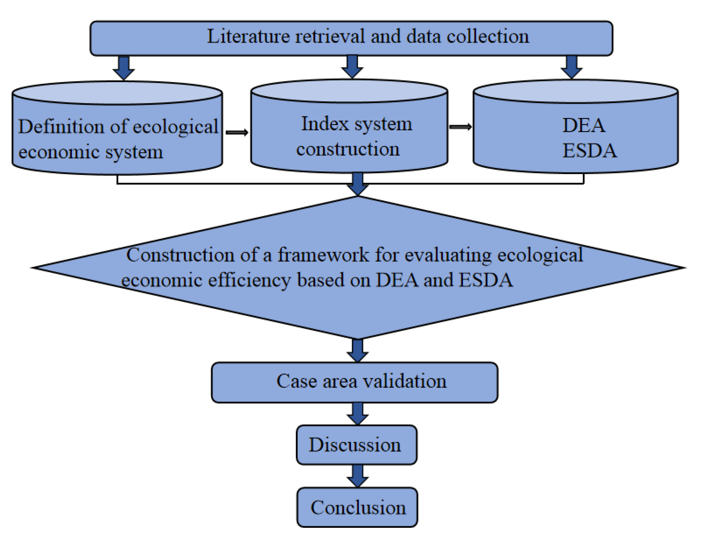
The remainder of this article is organized as follows: Section 3 presents the construction of the methodological framework and introduces the case areas and data sources; Section 4 provides an analysis of the calculation results; Section 5 provides the discussion and suggestions; and Section 6 presents the conclusions. Figure 2 presents the current study’s research process.
3. Materials and Methods
3.1. Research Methods
3.1.1. Construction of Index System
According to the connotation of an ecological economic system, this study established an index system for evaluating the efficiency of ecological economic mode from the three aspects of ecology, economy, and society (Table 2), namely input, desired output, and undesired output indicators.
3.1.2. SBM-DEA Model Containing Undesirable Output
This study established the SBM-CCR-DEA and SBM-BCC-DEA models, which contained undesired outputs, to measure the efficiency of ecological economic mode in the Huai River Basin, China. The model’s construction steps are as follows:
First, the municipal administrative unit was determined as the decision-making unit for evaluating the efficiency of ecological economic mode (, = 1, 2, …, ).
Second, an index system for evaluating the efficiency of ecological economic mode was established. The input indicator was marked as ; the desired output indicator was labeled as ; and the undesired output indicator was labeled as , where is the i-th input indicator of the j-th decision-making unit,= 1, 2, …, is the -th desired output indicator of the j-th decision-making unit, = 1, 2, …, ; and is the -th undesired output indicator of the j-th decision-making unit, = 1, 2, …, .
Third, the SBM-CCR-DEA model was constructed to measure the comprehensive efficiency of ecological economic mode, the equation for which is as follows:
In Equation (1), is the comprehensive efficiency of ecological economic mode in the evaluated unit (); ; is the slack variable of the input indicator; is the slack variable of the desired output indicator; is the slack variable of the undesired output indicator; and is the weight of .
Fourth, the SBM-BCC-DEA model was constructed to measure the technical efficiency of ecological economic mode, the equation for which was as follows:
In Equation (2), is the technical efficiency of ecological economic mode in .
Fifth, the scale efficiency of ecological economic mode was calculated on the basis of the SBM-CCR-DEA and SBM-BCC-DEA models. The equation was as follows:
In Equation (3), is the scale efficiency of ecological economic mode in .
3.1.3. Global Spatial Autocorrelation Index
The global spatial autocorrelation index (Moran I) reflects the overall spatial distribution characteristics about the efficiency of ecological economic mode in . An index value >0 indicates that adjacent decision-making units have similar ecological economic efficiency, that is, both decision-making units with high and low ecological economic efficiencies are clustered together. The greater the value is, the more obvious the spatial agglomeration phenomenon is. An index value <0 indicates that adjacent decision-making units have different ecological economic efficiencies, where the decision-making units with high and low ecological economic efficiencies exhibit an interval distribution. The larger the absolute value, the more obvious the spatial distribution phenomenon. An index value = 0 signifies that the correlation between adjacent decision-making units is low, and the decision-making units with high and low ecological economic efficiencies are randomly distributed. The equation for Moran I is as follows [35]:
In Equation (4), I is the global spatial autocorrelation index, n is the number of decision-making units, and are the ecological economic efficiency of the i-th and j-th decision-making units, respectively; is the average ecological economic efficiency, is the variance of ecological economic efficiency, and is a spatial weight matrix that conforms to the adjacency rule.
3.1.4. Local Spatial Autocorrelation Index
The local spatial autocorrelation index (Local Moran I) describes the degree of spatial agglomeration between similar levels of ecological economic efficiency around each decision-making unit. Additionally, it describes the degree of spatial differentiation between the ecological economic efficiencies of each decision-making unit and adjacent decision-making units, thereby revealing different forms of spatial connection. If the index value is >0, the ecological economic efficiency of the decision-making unit is similar to that of the adjacent units, demonstrating an agglomeration distribution state of decision-making units with similar attributes. If the index value is <0, the decision-making unit’s ecological economic efficiency is significantly different from that of adjacent units, exhibiting an interval distribution state of decision-making units with high attribute values and low attribute values. If index value =0, then the decision-making unit’s ecological economic efficiency has a low correlation with the ecological economic efficiency of adjacent units. Additionally, the decision-making units with higher and lower attribute values exhibit an irregular random distribution. The Local Moran I equation is as follows [36]:
In Equation (5), is the local spatial autocorrelation index, , and is limited to all adjacent units of the i-th decision-making unit.
3.2. Research Materials
3.2.1. Regional Overview
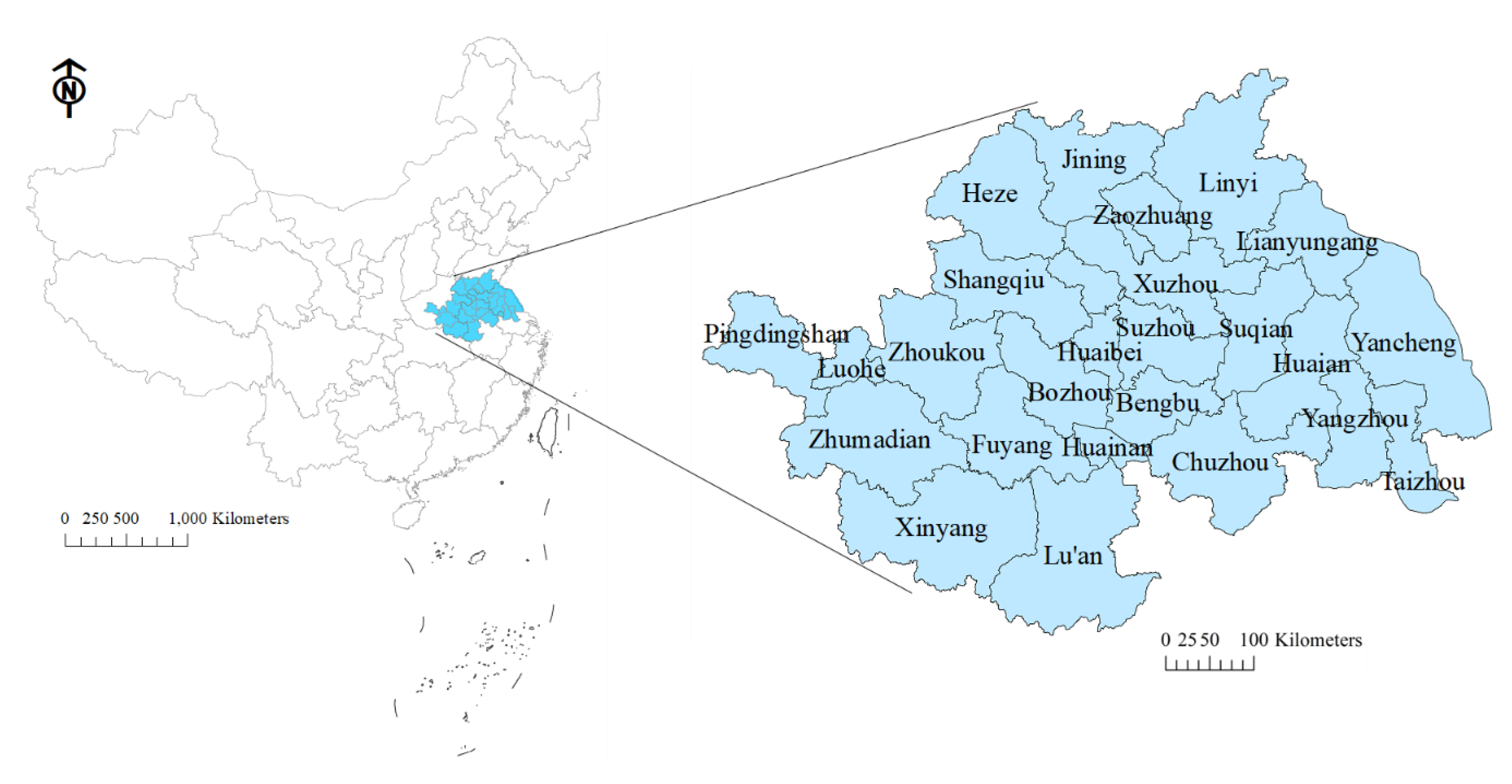
On 18 October 2018, the Huai River Ecological Economic Zone (Figure 3), based on the Huai River Basin, was reviewed as part of the State Council of the People’s Republic of China’s national strategy. The economic zone’s ecological resources are concentrated with low land development intensity, making it an excellent space for ecological economic development. The planned area of the Huai River Ecological Economic Zone is 243,000 square kilometers, with a permanent population of 146 million and a regional GDP of 6.75 trillion yuan. It will be built into a demonstration belt for the construction of ecological civilization in the basin and as the fourth growth pole after the Yangtze River Delta Economic Zone, Pearl River Delta economic zone, and Bohai Rim Economic Zone in China. The Huai River’s main stem, primary tributaries, and areas flowing through the downstream Yi-Shu-Si drainage system fall under the economic zone’s planning scope. This area comprises 25 cities and 4 counties in Jiangsu, Shandong, Anhui, Hubei, and Henan provinces (considering how the consistency of administrative areas enhances the comparability between spatial sequence data, the scope of the Huai River Ecological Economic Zone was revised to 25 cities).
3.2.2. Data Sources
Data on the number of days with excellent air quality and PM2.5 concentration of each city in 2018 were retrieved from the Statistical Bulletin on Environmental Quality and the statistical yearbooks of corresponding provinces in 2018.
4. Results
In this study, the ecological economic efficiencies of 25 cities in the Huai River Ecological Economic Zone were evaluated according to Equations (1)–(3) by using the MaxDEA Ultra7 software package (Beijing revomidi Software Co., Ltd., Beijing, China). Table 3 presents the evaluation results.
4.1. Analysis of Urban Ecological Economic Efficiency Types
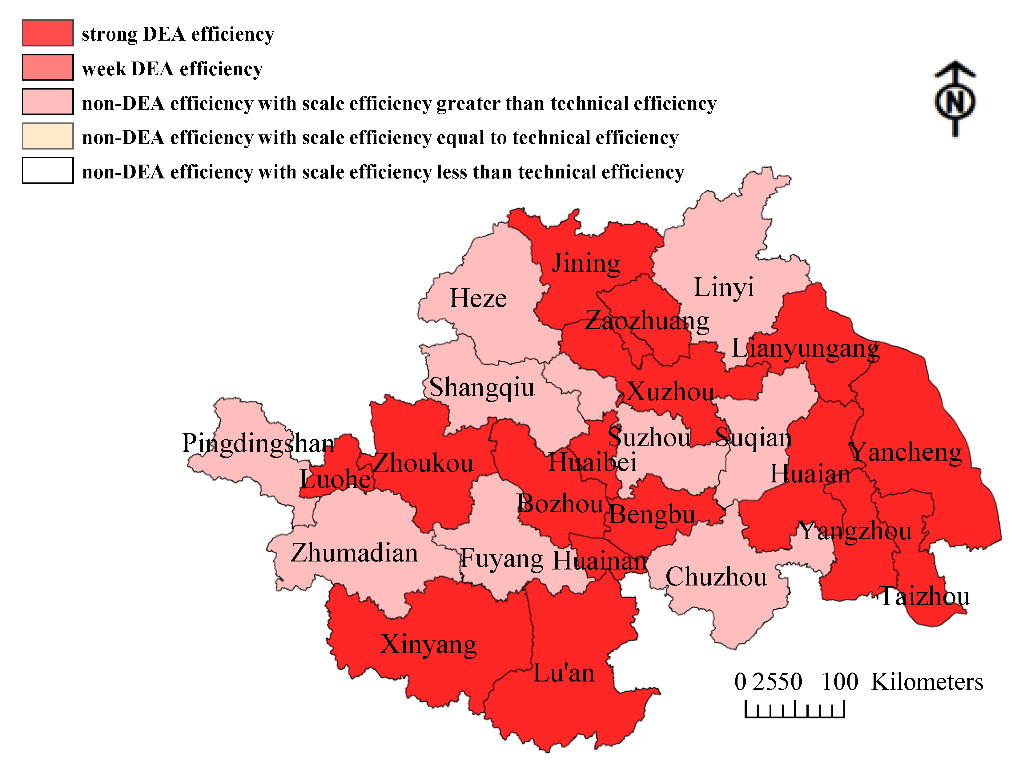
First, this study divided ecological economic comprehensive efficiency into DEA efficiency and non-DEA efficiency depending on whether the comprehensive efficiency value was equal to 1 or less than 1, respectively. Second, it subdivided DEA efficiency into strong and weak DEA efficiency depending on whether the conditions of were satisfied, respectively. Third, this study subdivided the non-DEA efficiency into scale efficiency > technical efficiency, scale efficiency = technical efficiency, and scale efficiency < technical efficiency according to the relationship between scale efficiency and technical efficiency. Finally, it used the urban ecological economic efficiency evaluation results to determine the types, and then used ARCGIS software for visualization; see Table 4 and Figure 4 for details.
As presented in Table 4 and Figure 4, the ecological economic efficiency of the cities in the economic zone could be classified into two categories: strong DEA efficiency and non-DEA efficiency, with scale efficiency > technical efficiency. The strong DEA efficiency cities were Xinyang, Zhoukou, Luohe, Bengbu, Huainan, Lu’an, Luzhou, Huaibei, Huaian, Yancheng, Xuzhou, Lianyungang, Yangzhou, Taizhou, Zaozhuang, and Jining, whereas the non-DEA efficiency cities were Zhumadian, Shangqiu, Pingdingshan, Fuyang, Suzhou, Chuzhou, Suqian, Linyi, and Heze.
4.2. Projection Analysis of Non-DEA Efficiency Urban Ecological Economic Efficiency
This study projected non-DEA efficiency urban ecological economic efficiency to analyze its causes and improvement values; Table 5 and Table 6 present the results. As seen in these tables, the input indicators of non-DEA efficiency urban ecological economic efficiency were redundant, the desired output indicators exhibited both optimal and insufficient conditions, and the undesired output indicators were in an excessive state.
Table 5 shows that the total redundancy of the non-DEA efficiency urban ecological economic efficiency input indicators was caused by radial redundancy and slack redundancy, and each input indicator had a different total redundancy, radial redundancy, and slack redundancy in each city. Total redundancy refers to the improvement value for the input indicators to reach the comprehensive efficiency DEA efficiency, radial redundancy refers to the improvement value for the input indicators to reach the scale efficiency DEA efficiency, and slack redundancy refers to the improvement value for the input indicators to achieve the technical efficiency DEA efficiency. From the total redundancy perspective of the input indicators, Linyi witnessed the greatest total redundancy in water, energy, land, labor, and capital resources, whereas Fuyang had the greatest total redundancy in the resource of public services. From the perspective of radial redundancy of the input indicators, Linyi exhibited the largest radial redundancy in the resources of water, energy, land, labor, capital, and public services. According to the slack redundancy of the input indicators, Zhumadian exhibited the greatest slack redundancy in water resources, Linyi exhibited the greatest slack redundancy in energy and land resources, and Fuyang exhibited the greatest slack redundancy in the resources of labor, capital, and public services.
As can be seen in Table 6, the desired output deficiency of non-DEA efficiency urban ecological economic efficiency was caused by slack deficiency, whereas the undesired output excess was caused by radial excess. Additionally, the total deficiency, radial deficiency, slack deficiency, the total excess, radial excess, and slack excess of each output indicator were different in each city. Total deficiency or total excess signifies the improvement values for the output indicators to achieve the comprehensive efficiency DEA efficiency, radial deficiency or radial excess refers to the improvement value for the output indicators to achieve the scale efficiency DEA efficiency, and slack deficiency or slack excess refers to the improvement value for the output indicators to reach the technical efficiency DEA efficiency. In terms of gross domestic product, the non-DEA efficiency urban output was optimal. Judging from the urbanization rate, all non-DEA efficiency urban output deficiencies comprised slack deficiencies, with Fuyang’s presenting the greatest output deficiency. On days with excellent air quality, all non-DEA efficiency urban output deficiencies comprised slack deficiencies, with Suzhou presenting the greatest deficiency. In terms of PM2.5 concentration, all non-DEA efficiency urban output excesses comprised radial excesses, with Linyi presenting the largest output excess.
4.3. Analysis of the Spatial Relationship of Urban Ecological Economic Efficiency
According to Equation (4), the global spatial autocorrelation indices of the comprehensive, technical, and scale efficiencies of the Huai River Ecological Economic Zone were −0.1004, −0.1053, and −0.1063, respectively. According to the results, the global spatial autocorrelation indices of comprehensive, technical, and scale efficiencies were all <0, indicating that the differences in comprehensive, technical, and scale efficiencies among adjacent decision-making units in the economic zone were all large and exhibited a state of interval distribution.
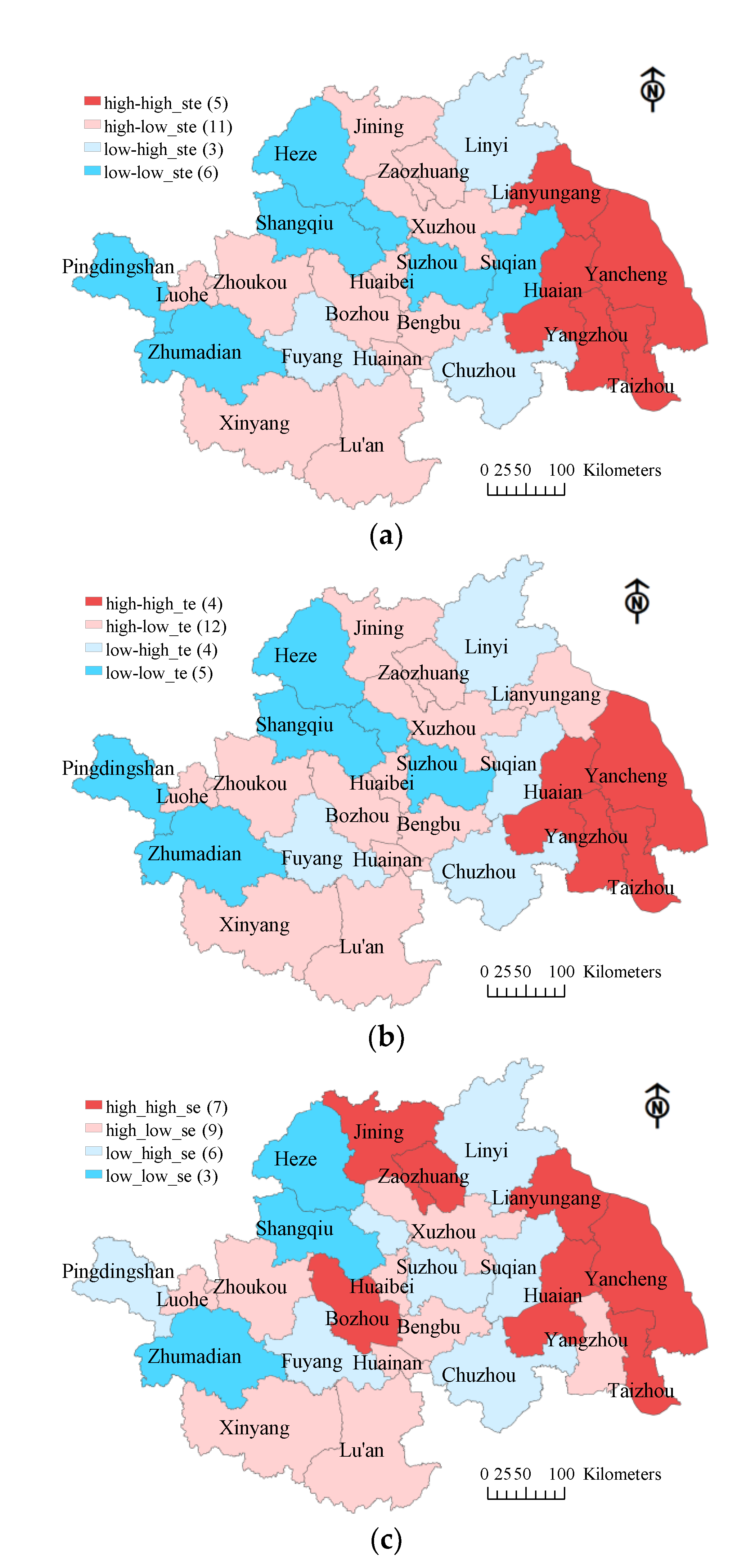
Furthermore, the local spatial autocorrelation indices of the comprehensive, technical, and scale efficiencies of the economic zone were calculated using Equation (5), which were then divided into positive and negative types depending on whether their values were greater than 0. Subsequently, they were divided into high and low values depending on whether the comprehensive, technical, and scale efficiencies were equal to 1. Finally, the divided types were superimposed to construct the spatial relationship between the comprehensive, technical, and scale efficiencies of the economic zone into high–high, low–low, low–high, and high–low cluster areas, as shown in Figure 5.
As can be seen in Figure 5, the overall spatial relationship trends of the comprehensive, technical, and scale efficiencies of the economic zone were similar; however, differences existed in the details. Among the four types, the high–high cluster areas were mainly distributed in the southeast region, the low–low cluster areas were generally distributed in the central and western regions, and the low–high and high–low cluster areas were scattered in between the aforementioned two regions. With respect to comprehensive efficiency (Figure 5a), the high–high cluster areas comprised five cities (e.g., Lianyungang), the high–low cluster areas comprised 11 cities (e.g., Jining), the low−high cluster areas comprised three cities (e.g., Linyi), and the low–low cluster areas comprised six cities (e.g., Suqian). With respect to technical efficiency (Figure 5b), the high–high cluster areas comprised four cities (e.g., Yancheng), the high−low cluster areas comprised 12 cities (e.g., Lianyungang), the low−high cluster areas comprised four cities (e.g., Suqian), and the low–low cluster areas comprised five cities (e.g., Suzhou). Moreover, regarding scale efficiency (Figure 5c), the high–high cluster areas comprised eight cities (e.g., Lianyungang), the high–low cluster areas comprised eight cities (e.g., Xuzhou), the low–high cluster areas comprised six cities (e.g., Suqian), and the low–low cluster areas comprised three cities (e.g., Shangqiu).
5. Discussion
This study constructed an index system and defined the methodological framework of DEA and ESDA for the efficiency monitoring of ecological economic mode on the basis of the connotation of an ecological economic system. Subsequently, it made an empirical study on the ecological economic efficiency of the Huai River Basin in China. The technical solutions can provide help for the government’s decision-making on the development of the basin.
The technical solutions can measure the ecological economic efficiencies of the basin and divide them into five categories, namely strong DEA efficiency, weak DEA efficiency, non-DEA efficiency with scale efficiency greater than technical efficiency, non-DEA effective with scale efficiency equal to technical efficiency, and non-DEA effective with scale efficiency less than technical efficiency. Based on this, the government can make strategic decisions to promote the ecological economic development of the basin and formulate comprehensive resource protection and development planning.
The technical solutions can reveal the causes of non-DEA efficiency on the ecological economic efficiency of the basin and give their optimal improvement values. The causes of non-DEA efficiency included redundant input, insufficient expected output, and excessive unexpected output. These results can help the government to make scientific decisions on how to control input and unexpected output and how to improve the expected output, so as to realize the efficient development of ecological economy in the basin.
The technical solutions can determine the spatial distribution of the ecological economic efficiency of the basin. The spatial distribution state included regular agglomeration distribution and irregular random distribution. The former included high ecological economic efficiency agglomeration area, low ecological economic efficiency agglomeration area, high ecological economic efficiency with low surrounding agglomeration area, and low ecological economic efficiency with high surrounding agglomeration area. According to these results, the government can make appropriate strategies for resource development and protection in different types of areas in the basin.
To summarize, the results of the empirical study by the technical solutions can provide a factual basis for the government to make decisions on the development and protection of the basin resources.
6. Conclusions
Considering the critical role of monitoring the efficiency of ecological economic mode in promoting the healthy development of China and rest of the world, this study constructed an index system on the basis of how the connotation of the ecological economic system is defined and built a framework comprising DEA and ESDA to measure the ecological economic efficiency of the Huai River Ecological Economic Zone in China and analyze its genesis and spatial relationships. The results revealed the following:
- (1)
- The ecological economic efficiency of the Huai River Basin in China was high as a whole. The ecological economic efficiencies of all cities respectively belonged to strong DEA efficiency type and non-DEA efficiency with scale efficiency greater than technical efficiency type, the former accounting for the majority.
- (2)
- The main causes of non-DEA efficiency in the Huai River Basin in China were redundant input of resources, insufficient output of days with good air quality, and excessive output of PM2.5, which were mainly caused by traditional industries with high energy consumption and high pollution.
- (3)
- The regional distribution of ecological economic efficiency in the Huai River Basin in China was unbalanced, the southeast of which became the agglomeration area of cities with high ecological economic efficiency by the advantage of coastal resources while the midwest became the agglomeration area of cities with low ecological economic efficiency due to its location in the interior.
From the conclusion of this study, several policy implications were obtained.
- (1)
- The government should promote the construction of green ecological corridor in the Huai River Basin in China. The ecological economic efficiency of the Huai River Basin is high as a whole, and its ecological economic development potential is huge. The government can build it into a green ecological corridor and a demonstration belt of ecological civilization. For a small number of cities, which are non-DEA efficiency with scale efficiency greater than technical efficiency, the government can to encourage R & D departments and scientific research institutions to innovate production technology by formulating policies of subsidy and tax reduction, so as to improve technical efficiency and then improve comprehensive efficiency.
- (2)
- The government should promote the industrial transformation and upgrading of the Huai River Basin in China. The traditional industries with large investment, high pollution, and low added value account for a large proportion in cities with non-DEA efficiency, which makes the ecological efficiency of these cities relatively low. On the premise of strengthening the protection of ecological environment, the government should develop their characteristic industries according to local conditions, and then accelerate the construction of modern industrial system with low energy consumption, low pollution, and high added value.
- (3)
- The government should make overall plans for the ecological economic development of various regions in the Huai River Basin in China. The southeast is the agglomeration area with high ecological economic efficiency while the central and western is the agglomeration area with low ecological economic efficiency. In order to achieve the common development of ecological economy in the basin, the government needs to formulate and implement resource and environment protection and development strategies for different regions. Industrial upgrading and factor diffusion should be promoted through structural optimization to achieve the leading of ecological economic efficiency in the southeast, while development efforts should be increased under the bearing capacity of resources and environment to achieve the improvement of ecological economic efficiency in the central and western parts.
This study sheds light on the overall level, types, causes, and spatial distribution characteristics of ecological economic efficiency in the Huai River Ecological Economic Zone in China. Our results provide useful information for the ecological economic development planning and policy formulation of the basin. However, this study had certain limitations. First, the selected indicators failed to present a full view of the ecological economic system. Under feasible conditions, the input and output indicators should be increased to comprehensively analyze efficiency of the ecological economic mode. Second, the study did not perform a dynamic analysis for evaluating efficiency of the ecological economic mode; thus, a time series DEA model should be constructed for dynamic analysis. Further work is required in these areas in the future.
Author Contributions
Conceptualization, C.Z.; methodology, C.Z.; software, C.Z. and G.M.; validation, C.Z. and C.W.; formal analysis, C.Z. and C.W.; investigation, W.-L.H. and M.W.; data curation, G.M. and M.W.; writing—review and editing, W.-L.H. All authors have read and agreed to the published version of the manuscript.
Funding
This research was funded by “Humanities and Social Sciences Foundation of the Chinese Ministry of Education, grant number 20YJA630087”, “Humanities and Social Sciences Foundation of the Chinese Ministry of Education, grant number 20YJAGAT002”, “National Natural Science Foundation of China, grant number 41271135”, “Humanities and Social Sciences Foundation of the Chinese Ministry of Education, grant number 18YJA790061”, and “Social Science Foundation of Jiangsu Province, China, grant number 18EYB008”.
Acknowledgments
We are grateful to the editor and anonymous reference for their comments. In addition, we would like to thank Yongyi Lu who studies in Huaiyin Normal University for her great contribution to the typesetting and proofreading of the article.
Conflicts of Interest
The authors declare no conflict of interest.
References
- Xu, J.; Jin, G.; Mo, Y.; Tang, H.; Li, L. Assessing Anthropogenic Impacts on Chemical and Biochemical Oxygen Demand in Different Spatial Scales with Bayesian Networks. Water 2020, 12, 246. [Google Scholar] [CrossRef] [Green Version]
- Zingaro, D.; Portoghese, I.; Giannoccaro, G. Modelling Crop Pattern Changes and Water Resources Exploitation: A Case Study. Water 2017, 9, 685. [Google Scholar] [CrossRef]
- Kucher, A.; Heldak, M.; Kucher, L.; Raszka, B. Factors Forming the Consumers’ Willingness to Pay a Price Premium for Ecological Goods in Ukraine. Int. J. Environ. Res. Public Health 2019, 16, 859. [Google Scholar] [CrossRef] [PubMed] [Green Version]
- Zhao, S.; Dong, G.; Xu, Y. A Dynamic Spatio-Temporal Analysis of Urban Expansion and Pollutant Emissions in Fujian Province. Int. J. Environ. Res. Public Health 2020, 17, 629. [Google Scholar] [CrossRef] [PubMed] [Green Version]
- Hou, J.; An, Y.; Song, H.; Chen, J. The Impact of Haze Pollution on Regional Eco-Economic Treatment Efficiency in China: An Environmental Regulation Perspective. Int. J. Environ. Res. Public Health 2019, 16, 4059. [Google Scholar] [CrossRef] [PubMed] [Green Version]
- Lauriola, P.; Crabbe, H.; Behbod, B.; Yip, F.; Medina, S.; Semenza, J.C.; Vardoulakis, S.; Kass, D.; Zeka, A.; Khonelidze, I.; et al. Advancing Global Health through Environmental and Public Health Tracking. Int J. Environ. Res. Public Health 2020, 17, 1976. [Google Scholar] [CrossRef] [Green Version]
- Polimeni, J.; Almalki, A.; Iorgulescu, R.; Albu, L.-L.; Parker, W.; Chandrasekara, R. Assessment of Macro-Level Socioeconomic Factors That Impact Waterborne Diseases: The Case of Jordan. Int. J. Environ. Res. Public Health 2016, 13, 1181. [Google Scholar] [CrossRef]
- Meyer, M.; Hirschnitz-Garbers, M.; Distelkamp, M. Contemporary Resource Policy and Decoupling Trends—Lessons Learnt from Integrated Model-Based Assessments. Sustainability 2018, 10, 1858. [Google Scholar] [CrossRef] [Green Version]
- McGee, M. The World’s CO2 Home Page. Available online: https://www.co2.earth/ (accessed on 24 April 2020).
- Duan, Y.; Xu, G.; Liu, Y.; Liu, Y.; Zhao, S.; Fan, X. Tendency of Runoff and Sediment Variety and Multiple Time Scale Wavelet Analysis in Hongze Lake during 1975–2015. Water 2020, 12, 999. [Google Scholar] [CrossRef] [Green Version]
- Liu, T.; Li, J.; Chen, J.; Yang, S. Urban Ecological Efficiency and Its Influencing Factors—A Case Study in Henan Province, China. Sustainability 2019, 11, 5048. [Google Scholar] [CrossRef] [Green Version]
- De Groot, R.S.; Fisher, B.; Christie, M.; Aronson, J.; Braat, L.; Haines-Young, R.; Gowdy, J.; Maltby, E.; Neuville, A.; Polasky, S. Integrating the ecological and economic dimensions in biodiversity and ecosystem service valuation. In The Economics of Ecosystems and Biodiversity (Teeb): Ecological and Economic Foundations; Earthscan, Routledge: London, UK, 2010; pp. 9–40. Available online: http://www.teebweb.org/our-publications/teeb-study-reports/ecological-and-economic-foundations/ (accessed on 30 July 2020).
- Berghöfer, A.; Mader, A.; Patrickson, S.; Calcaterra, E.; Smit, J.; Blignaut, J.; de Wit, M.; van Zyl, H. Teeb manual for cities: Ecosystem services in urban management. Econ. Ecosyst. Biodivers. Suiza; United Nations Environment Programme: Geneva, Switzerland, 2011. Available online: http://www.teebweb.org/publication/teeb-manual-for-cities-ecosystem-services-in-urban-management/ (accessed on 30 July 2020).
- Brink, P.; Berghöfer, A.; Schröter-Schlaack, C.; Sukhdev, P.; Vakrou, A.; White, S.; Wittmer, H. Teeb-the economics of ecosystems and biodiversity for national and international policy makers 2009. In TEEB-the Economics of Ecosystems and Biodiversity for National and International Policy Makers; United Nations Environment Programme: Geneva, Switzerland, 2009; Available online: http://www.teebweb.org/wp-content/uploads/Study%20and%20Reports/Reports/National%20and%20International%20Policy%20Making/TEEB%20for%20National%20Policy%20Makers%20report/TEEB%20for%20National.pdf (accessed on 30 July 2020).
- Leibenath, M.; Kurth, M.; Lintz, G. Science–Policy Interfaces Related to Biodiversity and Nature Conservation: The Case of Natural Capital Germany—TEEB-DE. Sustainability 2020, 12, 3701. [Google Scholar] [CrossRef]
- Lozano, R. Envisioning sustainability three-dimensionally. J. Clean. Prod. 2008, 16, 1838–1846. [Google Scholar] [CrossRef]
- Guo, Y.; Liu, W.; Tian, J.; He, R.; Chen, L. Eco-efficiency assessment of coal-fired combined heat and power plants in Chinese eco-industrial parks. J. Clean. Prod. 2017, 168, 963–972. [Google Scholar] [CrossRef]
- Schaltegger, S.; Sturm, A. Ecological rationality: Approaches to design of ecology-oriented management instruments. Die Unternehm. 1990, 4, 273–290. [Google Scholar]
- World Business Council for Sustainable Development. Eco-Efficient Leadership for Improved Economic and Environmental Performance; World Business Council for Sustainable Development: Geneva, Switzerland, 1995. [Google Scholar]
- Zhu, D.; Qiu, S. Eco-efficiency indicators and their demonstration as the circular economy measurement in China. Resour. Environ. Yangtze Basin 2008, 17, 1–5. [Google Scholar]
- Pan, X.X.; He, Y.Q.; Hu, X.F. Evaluation and spatial econometric analysis on regional ecological efficiency. Resour. Environ. Yangtze Basin 2013, 22, 640–647. [Google Scholar]
- Jiong, T. Application of Analytic Hierarchy Process in Eco-Efficiency Assessment. Environ. Prot. Sci. 2009, 1, 118–120. [Google Scholar]
- Lee, Y.-C. Ranking DMUs by Combining Cross-Efficiency Scores Based on Shannon’s Entropy. Entropy 2019, 21, 467. [Google Scholar] [CrossRef] [Green Version]
- Hao, Y.; Yang, D.; Yin, J.; Chen, X.; Bao, A.; Wu, M.; Zhang, X. The Effects of Ecological Policy of Kyrgyzstan Based on Data Envelope Analysis. Sustainability 2019, 11, 1922. [Google Scholar] [CrossRef] [Green Version]
- Mavi, R.K.; Saen, R.F.; Goh, M. Joint analysis of eco-efficiency and eco-innovation with common weights in two-stage network DEA: A big data approach. Technol. Forecast. And Soc. Chang. 2019, 144, 553–562. [Google Scholar] [CrossRef]
- Charnes, A.; Cooper, W.W.; Rhodes, E. Measuring the efficiency of decision making units. Eur. J. Oper. Res. 1978, 2, 429–444. [Google Scholar] [CrossRef]
- Rybaczewska-Błażejowska, M.; Gierulski, W. Eco-Efficiency Evaluation of Agricultural Production in the EU-28. Sustainability 2018, 10, 4544. [Google Scholar] [CrossRef] [Green Version]
- Wang, X.; Wu, Q.; Majeed, S.; Sun, D. Fujian’s Industrial Eco-Efficiency: Evaluation Based on SBM and the Empirical Analysis of lnfluencing Factors. Sustainability 2018, 10, 3333. [Google Scholar] [CrossRef] [Green Version]
- Bonfiglio, A.; Arzeni, A.; Bodini, A. Assessing eco-efficiency of arable farms in rural areas. Agric. Syst. 2017, 151, 114–125. [Google Scholar] [CrossRef]
- Tone, K. A slacks-based measure of efficiency in data envelopment analysis. Eur. J. Oper. Res. 2001, 130, 498–509. [Google Scholar] [CrossRef] [Green Version]
- Yu, J.; Zhou, K.; Yang, S. Regional heterogeneity of China’s energy efficiency in “new normal”: A meta-frontier Super-SBM analysis. Energy Policy 2019, 134, 110941. [Google Scholar] [CrossRef]
- Storto, C.l. Ecological Efficiency Based Ranking of Cities: A Combined DEA Cross-Efficiency and Shannon’s Entropy Method. Sustainability 2016, 8, 124. [Google Scholar] [CrossRef] [Green Version]
- Lv, X.; Lu, X.; Fu, G.; Wu, C. A Spatial-Temporal Approach to Evaluate the Dynamic Evolution of Green Growth in China. Sustainability 2018, 10, 2341. [Google Scholar] [CrossRef] [Green Version]
- Wei, G.; Sun, P.; Zhang, Z.; Ouyang, X. The Coordinated Relationship between Investment Potential and Economic Development and Its Driving Mechanism: A Case Study of the African Region. Sustainability 2020, 12, 442. [Google Scholar] [CrossRef] [Green Version]
- Moran, P.A. Notes on continuous stochastic phenomena. Biometrika 1950, 37, 17–23. [Google Scholar] [CrossRef] [PubMed]
- Anselin, L. Local indicators of spatial association—LISA. Geogr. Anal. 1995, 27, 93–115. [Google Scholar] [CrossRef]
Figure 1.
Evolution of the economic system; (a) conventional economic system [11]; (b) ecological economic system [5,16].

Figure 2.
Research process of this study. DEA: data envelopment analysis; ESDA: exploratory spatial data analysis.
Figure 2.
Research process of this study. DEA: data envelopment analysis; ESDA: exploratory spatial data analysis.

Figure 3.
Location and administrative areas of the Huai River Ecological Economic Zone.

Figure 4.
Types of urban ecological economic efficiencies in the Huai River Ecological Economic Zone.
Figure 4.
Types of urban ecological economic efficiencies in the Huai River Ecological Economic Zone.

Figure 5.
Analysis of the spatial relationship of ecological economic efficiency; (a) spatial relationship of comprehensive efficiency; (b) spatial relationship of technical efficiency; (c) spatial relationship of scale efficiency.
Figure 5.
Analysis of the spatial relationship of ecological economic efficiency; (a) spatial relationship of comprehensive efficiency; (b) spatial relationship of technical efficiency; (c) spatial relationship of scale efficiency.


Table 1.
Overview of index systems and methods for evaluating ecological economic efficiency.
| Authors | Indicators | Methods | Results | |||
|---|---|---|---|---|---|---|
| Input Indicators | Output Indicators | |||||
| Desired Outputs | Undesired Outputs | |||||
| A. Bonfiglio, A. Arzeni, A. Bodini (2017) [29] | specialization index, nitrogen balance, phosphorus balance, pesticide risk | added value | - | CCR | to reflect the DMUs’ comprehensive efficiencies | |
| M. Rybaczewska- Błażejowska, W. Gierulski (2018) [27] | a set of impact categories from the life cycle assessment stage | economic indicator | - | BCC | to reflect the DMUs’ technical efficiencies | |
| X. Wang, Q. Wu, S. Majeed, D. Sun (2018) [28] | the consumption of standard coal, the consumption of fresh water | industrial added value | I | SBM | to reduce deviations on the DMUs’ efficiency evaluations | |
| Y. Hao, D. Yang, J. Yin, X. Chen, A. Bao, M. Wu, et al. (2019) [24] | total water diversion, air pollutant emission from fixed sources | GDP per capita, afforestation, non-poverty rate | - | S-CCR | to further distinguish the significant degrees of the DMUs in strongly valid states | |
| J. Yu, K. Zhou, and S. Yang (2019) [31] | labor, capital, energy | gross domestic product | CO2 emissions | S-SBM | ||
| C. lo Storto (2016) [32] | population, land area | II | III | C-SBM | to further distinguish the significant degrees of the DMUs in valid states | |
| R. Kiani Mavi, R. F. Saen, and M. Goh (2019) [25] | ecological efficiency stage | labor force, energy use, land area | GDP | GHG emissions | N-SBM | to study the impact of each link on ecological efficiency in the process |
| ecological innovation stage | GDP, GHG emissions | IV | - | |||
Note: I indicates the discharge amount of industrial wastewater, the emission amount of industrial waste gas; II indicates the number of residents enjoying black water purification service, the amount of urban garbage collected by classification, the total power of photovoltaic power stations installed on the roofs of public buildings, the total amount of urban green space available to the public, the number of public transport passengers, and the number of vehicles classified as pollution-free; III indicates household water consumption, unclassified urban garbage collection, household natural gas consumption, household electricity consumption, days when the air quality threshold of particulate matter with less than or equal to 10 microns in diameter (PM10) exceeds and the number of vehicles classified as polluted; IV indicates researchers in R & D, high technology export, electricity production from renewable sources, and the number of ISO 14001 certificates. GDP: gross domestic product; GHG: greenhouse gas; CCR: Charnes–Cooper–Rhodes; DMU: decision-making unit; BCC: Banker–Charnes–Cooper; SBM: slacks-based measure; S-CCR: super-efficiency CCR; C-SBM: cross-efficiency SBM; N-SBM: network-efficiency SBM.
Table 2.
Construction of the index system for evaluating the efficiency of ecological economic mode.
Table 2.
Construction of the index system for evaluating the efficiency of ecological economic mode.
| Indicator Type | Indicator Property | Indicator Composition | Indicator Meaning | |
|---|---|---|---|---|
| Input indicator | Ecological input | Total water resources (100 million m3) | Water input | |
| Total electricity consumption of the society (100 million kWh) | Energy input | |||
| Total land area (km2) | Land input | |||
| Economic input | Number of employees (10,000 people) | Labor input | ||
| Loans in Renminbi and foreign currencies of all financial institutions at year-end (¥100 million) | Capital input | |||
| Social input | General budget expenditure (¥100 million) | Public service input | ||
| Output indicator | Desired output indicator | Ecological output | Excellent air quality (day) | Excellent environmental output |
| Economic output | Gross domestic product (¥100 million) | Product and service outputs | ||
| Social output | Urbanization rate (%) | Urban resident output | ||
| Undesired output indicator | Ecological output | PM2.5 concentration (μg/m3) | Waste output | |
Table 3.
Related parameters for evaluating the efficiency of ecological economic mode.
| Province | City | |||||
|---|---|---|---|---|---|---|
| Henan | Xinyang | 1.00 | 1.00 | 1.00 | 0 | 0 |
| Zhumadian | 0.82 | 0.85 | 0.97 | 3499 | 13 | |
| Zhoukou | 1.00 | 1.00 | 1.00 | 0 | 0 | |
| Luohe | 1.00 | 1.00 | 1.00 | 0 | 0 | |
| Shangqiu | 0.78 | 0.80 | 0.98 | 2854 | 10 | |
| Pingdingshan | 0.81 | 0.86 | 0.94 | 1913 | 25 | |
| Anhui | Bengbu | 1.00 | 1.00 | 1.00 | 0 | 0 |
| Huainan | 1.00 | 1.00 | 1.00 | 0 | 0 | |
| Fuyang | 0.72 | 0.79 | 0.95 | 458 | 40 | |
| Lu’an | 1.00 | 1.00 | 1.00 | 0 | 0 | |
| Bozhou | 1.00 | 1.00 | 1.00 | 0 | 0 | |
| Suzhou | 0.74 | 0.82 | 0.90 | 2056 | 52 | |
| Huaibei | 1.00 | 1.00 | 1.00 | 0 | 0 | |
| Chuzhou | 0.78 | 0.84 | 0.93 | 3963 | 36 | |
| Jiangsu | Huai’an | 1.00 | 1.00 | 1.00 | 0 | 0 |
| Yancheng | 1.00 | 1.00 | 1.00 | 0 | 0 | |
| Suqian | 0.91 | 0.92 | 0.99 | 1080 | 5 | |
| Xuzhou | 1.00 | 1.00 | 1.00 | 0 | 0 | |
| Lianyungang | 1.00 | 1.00 | 1.00 | 0 | 0 | |
| Yangzhou | 1.00 | 1.00 | 1.00 | 0 | 0 | |
| Taizhou | 1.00 | 1.00 | 1.00 | 0 | 0 | |
| Shandong | Zaozhuang | 1.00 | 1.00 | 1.00 | 0 | 0 |
| Jining | 1.00 | 1.00 | 1.00 | 0 | 0 | |
| Linyi | 0.71 | 0.72 | 0.98 | 7239 | 27 | |
| Heze | 0.74 | 0.78 | 0.96 | 4279 | 45 |
Note: ste is the comprehensive efficiency; te is the technical efficiency; se is the scale efficiency; is the slack variable of input indicator; is the slack variable of the output indicator; and .
Table 4.
Type division of ecological economic efficiency.
| Type | City | |
|---|---|---|
| DEA efficiency () | Strong DEA efficiency () | Xinyang, Zhoukou, Luohe, Bengbu, Huainan, Lu’an, Bozhou, Huaibei, Huai’an, Yancheng, Xuzhou, Lianyungang, Yangzhou, Taizhou, Zaozhuang, Jining |
| Weak DEA efficiency (Except ) | - | |
| Non-DEA efficiency () | Scale efficiency is greater than technical efficiency () | Zhumadian, Shangqiu, Pingdingshan, Fuyang, Suzhou, Chuzhou, Suqian, Linyi, Heze |
| Scale efficiency is equal to technical efficiency () | - | |
| Scale efficiency is less than technical efficiency () | - | |
Table 5.
Analysis of redundant input in non-DEA efficiency cities.
| Input Redundancy and Subitems | Henan | Anhui | Jiangsu | Shandong | |||||||
|---|---|---|---|---|---|---|---|---|---|---|---|
| Zhuma Dian | Shang Qiu | Pingding Shan | Fu Yang | Su Zhou | Chu Zhou | Su Qian | Lin Yi | He Ze | |||
| Ecological input | Water resources | Radial redundancy | −4.23 | −1.34 | −3.08 | −9.14 | −0.65 | −1.86 | −0.05 | −10.06 | −2.73 |
| Slack redundancy | −16.76 | 0.00 | 0.00 | −2.52 | 0.00 | −0.85 | −7.34 | −13.01 | 0.00 | ||
| Total redundancy | −20.99 | −1.34 | −3.08 | −11.66 | −0.65 | −2.71 | −7.39 | −23.07 | −2.73 | ||
| Energy | Radial redundancy | −10.62 | −12.18 | −28.65 | −23.90 | −1.70 | −6.29 | −0.27 | −108.35 | −26.94 | |
| Slack redundancy | −9.82 | −56.49 | −20.23 | 0.00 | 0.00 | −37.86 | 0.00 | −120.08 | −27.60 | ||
| Total redundancy | −20.44 | −68.67 | −48.88 | −23.90 | −1.70 | −44.16 | −0.27 | −228.43 | −54.54 | ||
| Land resources | Radial redundancy | −1288 | −723 | −1323 | −1868 | −213 | −558 | −13 | −4252 | −1609 | |
| Slack redundancy | −3444 | −2585 | −1832 | 0 | −1971 | −3878 | −1032 | −6847 | −4098 | ||
| Total redundancy | −4732 | −3308 | −3155 | −1868 | −2185 | −4436 | −1046 | −11099 | −5707 | ||
| Economic input | Labor | Radial redundancy | −51.74 | −39.73 | −57.55 | −128.71 | −8.30 | −12.14 | −0.44 | −170.37 | −67.68 |
| Slack redundancy | −28.47 | −153.73 | −61.10 | −291.97 | −52.59 | 0.00 | 0.00 | −258.27 | −112.55 | ||
| Total redundancy | −80.20 | −193.46 | −118.65 | −420.68 | −60.88 | −12.14 | −0.44 | −428.64 | −180.23 | ||
| Capital | Radial redundancy | −121.13 | −96.71 | −289.72 | −393.09 | −27.23 | −70.92 | −3.47 | −1109.76 | −264.32 | |
| Slack redundancy | 0.00 | 0.00 | 0.00 | −50.28 | 0.00 | 0.00 | 0.00 | 0.00 | 0.00 | ||
| Total redundancy | −121.13 | −96.71 | −289.72 | −443.37 | −27.23 | −70.92 | −3.47 | −1109.76 | −264.32 | ||
| Social input | Public services | Radial redundancy | −40.75 | −31.27 | −53.29 | −98.48 | −7.54 | −15.87 | −0.66 | −145.90 | −67.08 |
| Slack redundancy | 0.00 | −58.95 | 0.00 | −113.20 | −32.16 | −46.27 | −40.36 | 0.00 | −41.14 | ||
| Total redundancy | −40.75 | −90.22 | −53.29 | −211.69 | −39.70 | −62.14 | −41.02 | −145.90 | −108.22 | ||
Note: Radial redundancy refers to the improvement value for the input indicators to reach the scale efficiency DEA efficiency, slack redundancy refers to the improvement value for the input indicators to achieve the technical efficiency DEA efficiency, and total redundancy refers to the improvement value for the input indicators to reach the comprehensive efficiency DEA efficiency.
Table 6.
Analysis of deficient or excessive output in non-DEA efficiency cities.
| Output Deficiency (or Excess) and Subitems | Henan | Anhui | Jiangsu | Shandong | ||||||||
|---|---|---|---|---|---|---|---|---|---|---|---|---|
| Zhuma Dian | Shang Qiu | Pingding Shan | Fu Yang | Su Zhou | Chu Zhou | Su Qian | Lin Yi | He Ze | ||||
| Desired output | Economic output | Gross domestic product | Radial deficiency | 0.00 | 0.00 | 0.00 | 0.00 | 0.00 | 0.00 | 0.00 | 0.00 | 0.00 |
| Slack deficiency | 0.00 | 0.00 | 0.00 | 0.00 | 0.00 | 0.00 | 0.00 | 0.00 | 0.00 | |||
| Total deficiency | 0.00 | 0.00 | 0.00 | 0.00 | 0.00 | 0.00 | 0.00 | 0.00 | 0.00 | |||
| Social output | Urbanization rate | Radial deficiency | 0.00 | 0.00 | 0.00 | 0.00 | 0.00 | 0.00 | 0.00 | 0.00 | 0.00 | |
| Slack deficiency | 5.94 | 9.93 | 7.61 | 14.90 | 12.02 | 3.96 | 1.05 | 11.80 | 12.63 | |||
| Total deficiency | 5.94 | 9.93 | 7.61 | 14.90 | 12.02 | 3.96 | 1.05 | 11.80 | 12.63 | |||
| Ecological output | Excellent air quality days | Radial deficiency | 0.00 | 0.00 | 0.00 | 0.00 | 0.00 | 0.00 | 0.00 | 0.00 | 0.00 | |
| Slack deficiency | 7.11 | 0.00 | 16.93 | 25.45 | 39.62 | 31.94 | 4.05 | 15.08 | 31.96 | |||
| Total deficiency | 7.11 | 0.00 | 16.93 | 25.45 | 39.62 | 31.94 | 4.05 | 15.08 | 31.96 | |||
| Undesired output | PM2.5 Concentration | Radial excess | −6.40 | −5.13 | −13.42 | −12.80 | −1.42 | −2.29 | −0.08 | −19.05 | −10.91 | |
| Slack excess | 0.00 | 0.00 | 0.00 | 0.00 | 0.00 | 0.00 | 0.00 | 0.00 | 0.00 | |||
| Total excess | −6.40 | −5.13 | −13.42 | −12.80 | −1.42 | −2.29 | −0.08 | −19.05 | −10.91 | |||
Note: Radial deficiency or radial excess refers to the improvement value for the output indicators to achieve the scale efficiency DEA efficiency, slack deficiency or slack excess refers to the improvement value for the output indicators to reach the technical efficiency DEA efficiency, and total deficiency or total excess signifies the improvement values for the output indicators to achieve the comprehensive efficiency DEA efficiency.
© 2020 by the authors. Licensee MDPI, Basel, Switzerland. This article is an open access article distributed under the terms and conditions of the Creative Commons Attribution (CC BY) license (http://creativecommons.org/licenses/by/4.0/).
Share and Cite
MDPI and ACS Style
Zhang, C.; Wang, C.; Mao, G.; Wang, M.; Hsu, W.-L. An Empirical Study on the Ecological Economy of the Huai River in China. Water 2020, 12, 2162. https://0-doi-org.brum.beds.ac.uk/10.3390/w12082162
AMA Style
Zhang C, Wang C, Mao G, Wang M, Hsu W-L. An Empirical Study on the Ecological Economy of the Huai River in China. Water. 2020; 12(8):2162. https://0-doi-org.brum.beds.ac.uk/10.3390/w12082162
Chicago/Turabian StyleZhang, Chunmei, Chengxiang Wang, Guangxiong Mao, Min Wang, and Wei-Ling Hsu. 2020. "An Empirical Study on the Ecological Economy of the Huai River in China" Water 12, no. 8: 2162. https://0-doi-org.brum.beds.ac.uk/10.3390/w12082162
Note that from the first issue of 2016, this journal uses article numbers instead of page numbers. See further details here.