Climate Change Impacts on Soil Erosion and Sediment Yield in a Watershed


1
Department of Tropical Agriculture and International Cooperation, National Pingtung University of Science and Technology, Pingtung 91201, Taiwan
2
Department of Soil and Water Conservation, National Chung Hsing University, Taichung 40227, Taiwan
3
Research and Development Foundation, National Cheng-Kung University, Tainan 70101, Taiwan
*
Author to whom correspondence should be addressed.
Water 2020, 12(8), 2247; https://0-doi-org.brum.beds.ac.uk/10.3390/w12082247
Submission received: 2 July 2020
/
Revised: 7 August 2020
/
Accepted: 7 August 2020
/
Published: 10 August 2020
(This article belongs to the Special Issue Soil–Water Conservation, Erosion, and Landslide)
Abstract
:This study analyzed the influence of climate change on sediment yield variation, sediment transport and erosion deposition distribution at the watershed scale. The study was based on Gaoping River basin, which is among the largest basins in southern Taiwan. To carry out this analysis, the Physiographic Soil Erosion Deposition (PSED) model was utilized. Model results showed a general increase in soil erosion and deposition volume under the A1B-S climate change scenario. The situation is even worsened with increasing return periods. Total erosion volume and total sediment yield in the watershed were increased by 4–25% and 8–65%, respectively, and deposition volumes increased by 2–23%. The study showed how climate change variability would influence the watershed through increased sediment yields, which might even worsen the impacts of natural disasters. It has further illustrated the importance of incorporating climate change into river management projects.
1. Introduction
Due to the increasing severity of global warming and climate change effect in recent years, extreme hydrographic phenomena have frequently been observed. Climate change has increased precipitation concentration, volume and intensity, which has significantly impacted runoff and soil erosion in many watersheds [1,2,3]. The sediments generated from watershed erosion are transported to rivers via surface runoff, and they are the main composition of river sediments and a major source of reservoir or river dam sediment deposition [4]. The degree of soil erosion has a significant impact on the evolution of river channels, influencing river stability, flood prevention safety and river remediation planning. Hence, the control of sediment yield is crucial in watershed management, especially since it usually involves high costs. In a review of sediment management strategies in Taiwan and the barriers to their implementation, Wang et al. [5] highlighted how technical barriers are driven primarily by engineering and costs. This was in reference to methods such as construction of upstream sediment structures and hydraulic and mechanical dredging. Moreover, in some regions, climate change is projected to decrease the overall soil erosion potential due to decrease in rainfall [6].
Several studies have focused on the impacts of climate change on precipitation volume, runoff volume, erosion volume and sediment yield. General Circulation Models (GCMs) have been applied to analyze the impacts of climate change on precipitation characteristic [7,8,9] and river runoff [10,11]. The Soil and Water Assessment Tool (SWAT) model seems to be the most favored by researchers when evaluating the impacts of climate change on flow rate, soil erosion and sediment yield in a watershed area [12,13]. Thodsen et al. [14] applied the High Resolution Limited Area Model (HIRHAM) regional climate model to investigate the impact of climate change on suspended load transport rate of Danish rivers. In modeling flow rate and sediment yield for high flow-rate rivers under the A2 scenario in the rain season of 2050, Phan et al. [15] showed an increase of 11.4% and 15.3%, respectively. Cousino et al. [16] utilized SWAT to provide hydrological insights for the Maumee River watershed, showing a reduction by 10% in flow, while sediment yield increased by 11%. Most recently, Zhou et al. [17] used the SWAT model to evaluate the impacts of climate change on flow and sediment yield in northeast China. In northern Iran, Azari et al. [18] reported an annual increase of 5% in annual streamflow and more than 35% in sediment yield. Zhang et al. [19] generated climatic conditions for future periods 2020–2039, 2050–2069 and 2080–2099, and their results demonstrated an increase of 13% in sediment yield.
The abovementioned methods do not couple the computations of slope erosion and river sediment transport. Instead, watershed erosion is calculated first based on slope information, followed by watershed sediment yield based on sediment delivery ratio, a river sediment transport model or runoff volume with a flow rate-sediment transport rating curve. The estimation of slope erosion, regardless of applying the Universal Soil Loss Equation (USLE), Revised Universal Soil Loss Equation (RUSLE) [20] or Modified Universal Soil Loss Equation (MUSLE), is carried out by empirical model. Empirical models are established based on erosion data of the initial location via inductive analysis. Therefore, they have application and location limitations. Moreover, the erosion volume estimated by empirical models is the total erosion volume rather than the time-dependent or spatial-dependent erosion volume. Furthermore, watersheds and river systems are complex and sediment boundary conditions for carrying out river sediment transport simulations by the abovementioned models cannot be obtained directly. Typically, sediment transport volume is estimated by the flow rate-sediment transport rating curves established through hydrological observation stations. Nonetheless, sediment transport rates estimated by rating curves have large uncertainties, especially with high discharge values [21].
To understand the impacts of climate change on erosion volume, sediment yield and erosion distribution for a watershed, this study utilized a Physiographic Soil Erosion-Deposition (PSED) model proposed by Chen, Tsai and Tsai [4]. Unlike empirical models, the PSED model has physical mechanisms that enable simultaneous computation of slope erosion and river sediment transport. Additionally, this model does not require the flow rate-sediment rating curve as a boundary condition, thus eliminating uncertainties that come with their adoption. Findings from this study will serve as a useful reference for decision-making authorities in planning appropriate strategies and corresponding measures to prevent water- and soil-related disasters.
2. Materials and Methods
2.1. Study Area
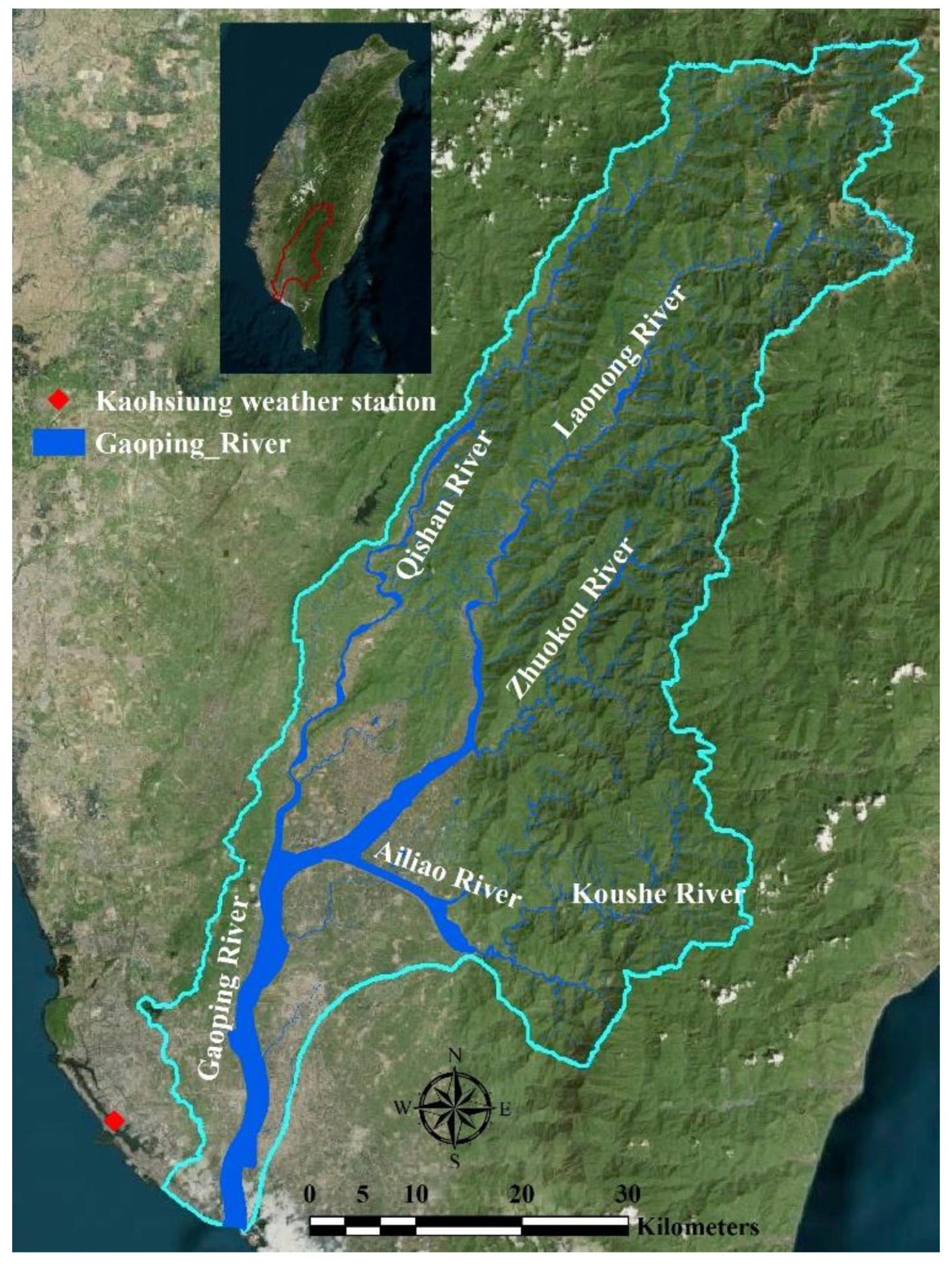
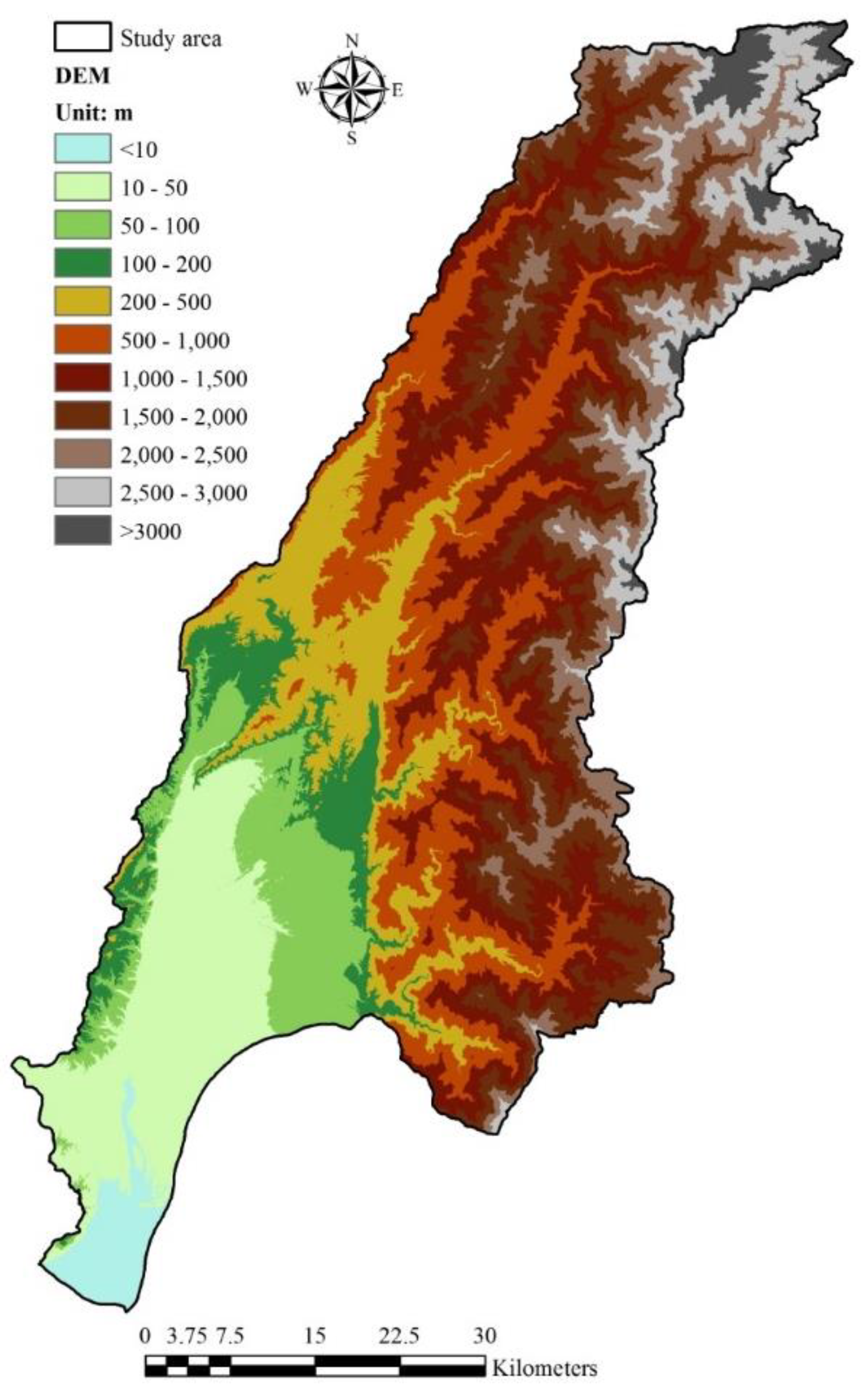
Gaoping River, which is the largest river in Taiwan, was used for the analysis. It is located in the southwest of Taiwan and has a total length of 171 km, covering 3257 km2. It originates from west of the Central Mountain Range near Yushan. The upstream end is connected to Laonong River, and its main branches include Qishan, Ailiao and Zhuokou (Figure 1). The topographic height varies significantly, descending along the direction from northeast to southwest, with a maximum difference of nearly 4000 m. The area above 1000 m accounts for 47.45% of the total drainage basin, that between 100 and 1000 m accounts for 32.38% and finally, the area below 100 m accounts for 20.17%. The average slope of the river bed is approximately 1/150, with 1/15, 1/100 and 1/1000 for the upstream, midstream and downstream sections, respectively. Additionally, the sections’ lengths are 37, 68 and 66 km for the upstream, midstream and downstream sections, respectively.
Time- and location-based precipitation distribution in the basin varies widely. Near the Central Mountain Range it is large (~3400 mm), whereas in the plain and coastal areas it is significantly smaller (~2000 mm). Precipitation is concentrated from May to October, which accounts for 90% of the annual precipitation. Average annual runoff volume is ~8.45 billion m3, of which 7.69 billion m3 (91%) occur in the wet season. The average annual sediment transport volume is 35.61 million tons, with 10,934 tons of sediment transport per km2 of drainage basin area.
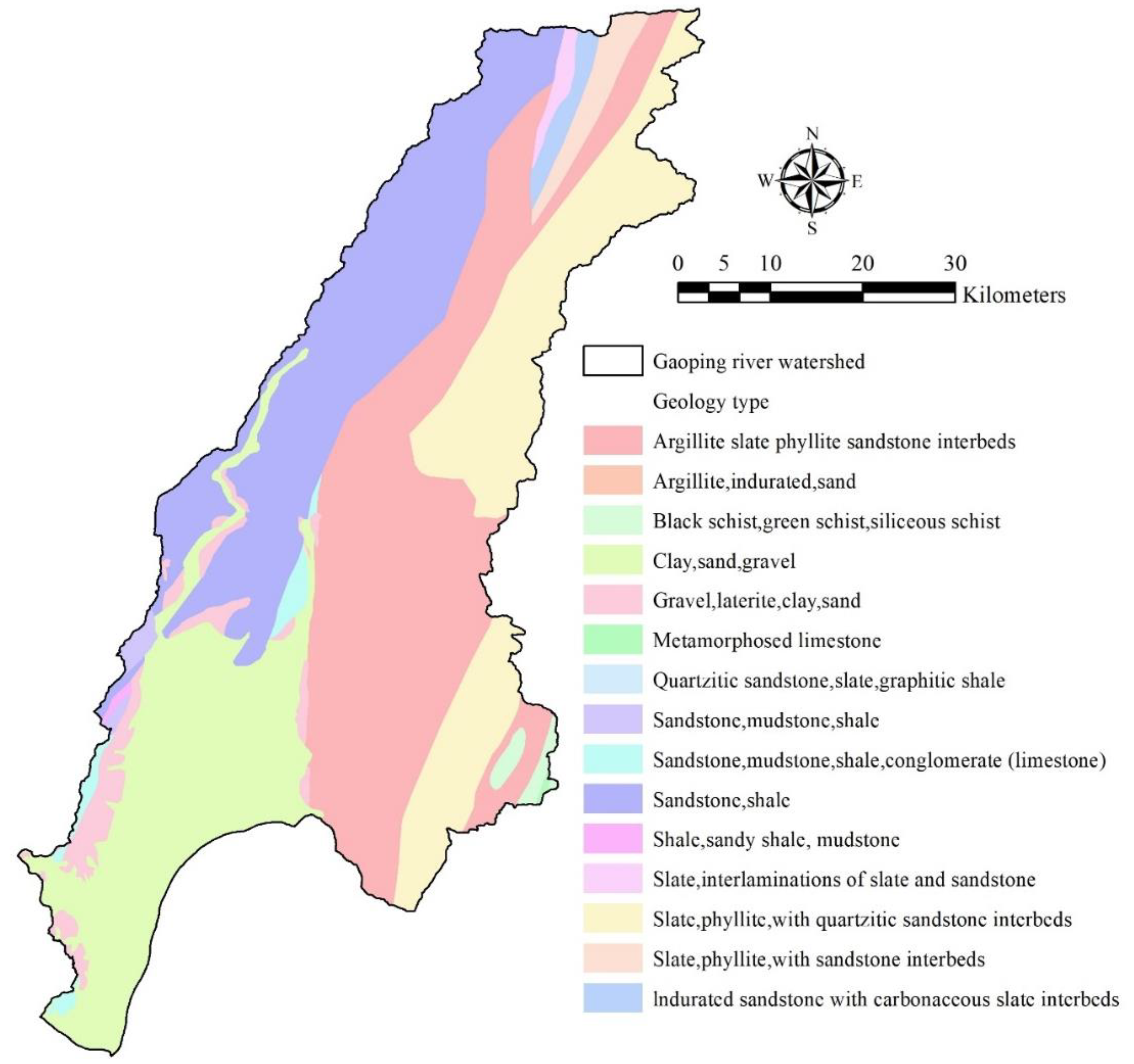
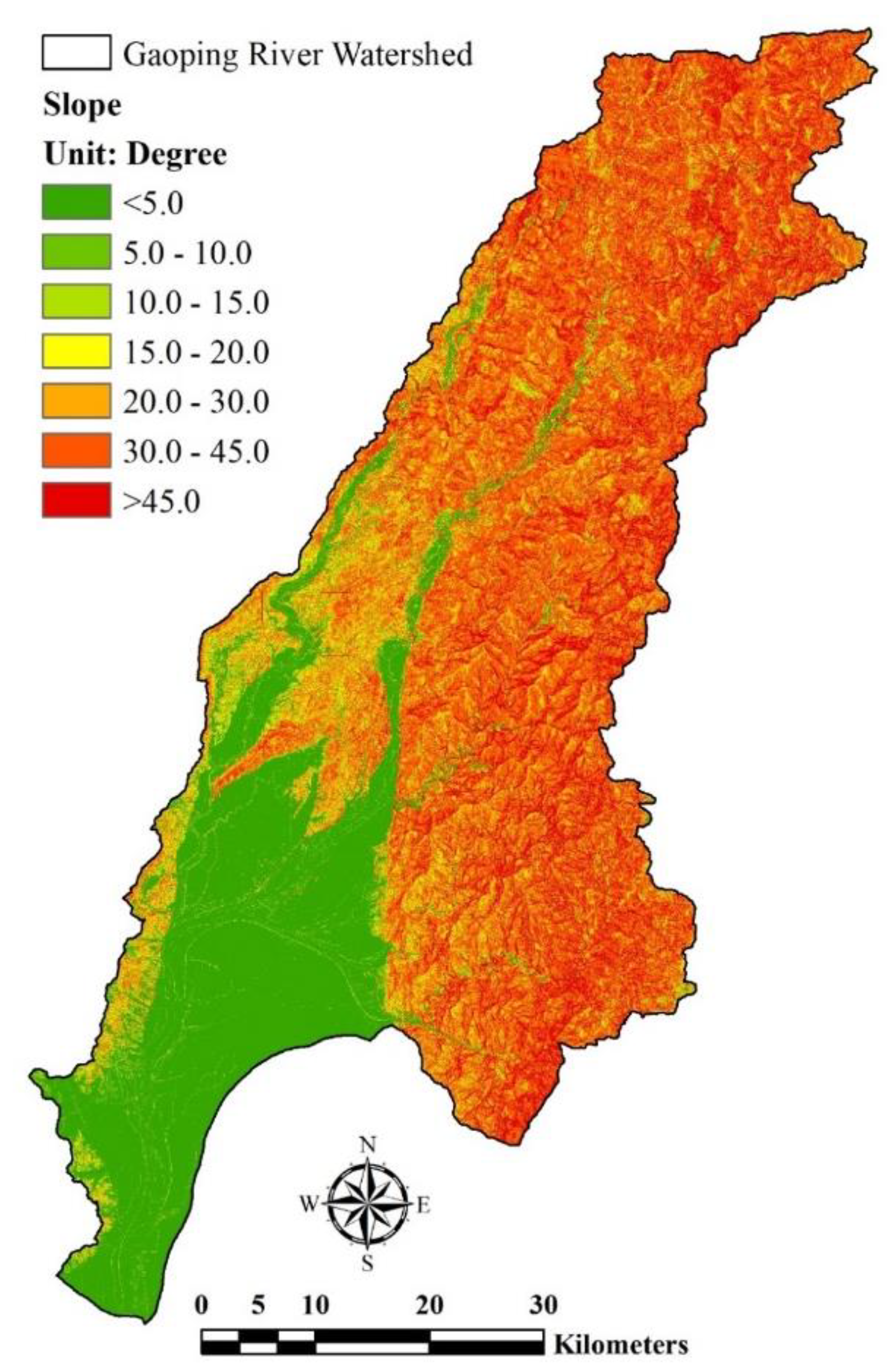
The Gaoping River basin is among the worst basins in Taiwan in terms of sediment yield and is highly vulnerable to sediment deposition. Statistical data from the Water Resources Agency of Taiwan, MOEA, estimate a total dredging sediment volume of 94,780,000 m3 for Gaoping River basin between 2009 to 2014 [22]. The major contributions to such high rates include the high-slope landform and concentrated precipitation. The geological map in Figure 2 shows that the watershed mainly constitutes sand gravel and sandstone, rendering it vulnerable to erosion. Stefanidis and Stathis [6], in their assessment of soil erosion in a catchment, showed that vulnerable geological subsoil and the steep slopes favor the development of erosion phenomena. At Gaoping, about 80% of the annual precipitation is from an average of 3–4 typhoons per year [21], which fall between June and September each year. Precipitation in these events is characterized by high intensity and short duration, leading to enormous volumes of sediment yield. The situation is even worsened by additional factors, such as climate change, which has caused drastic changes in precipitation [23].
2.2. Long Term Climate and Hydrological Changes
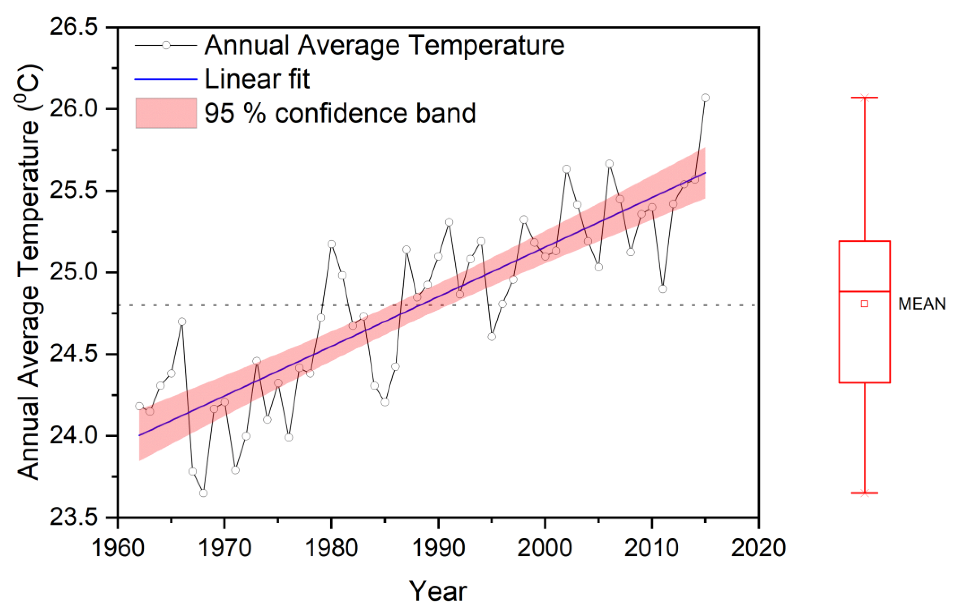
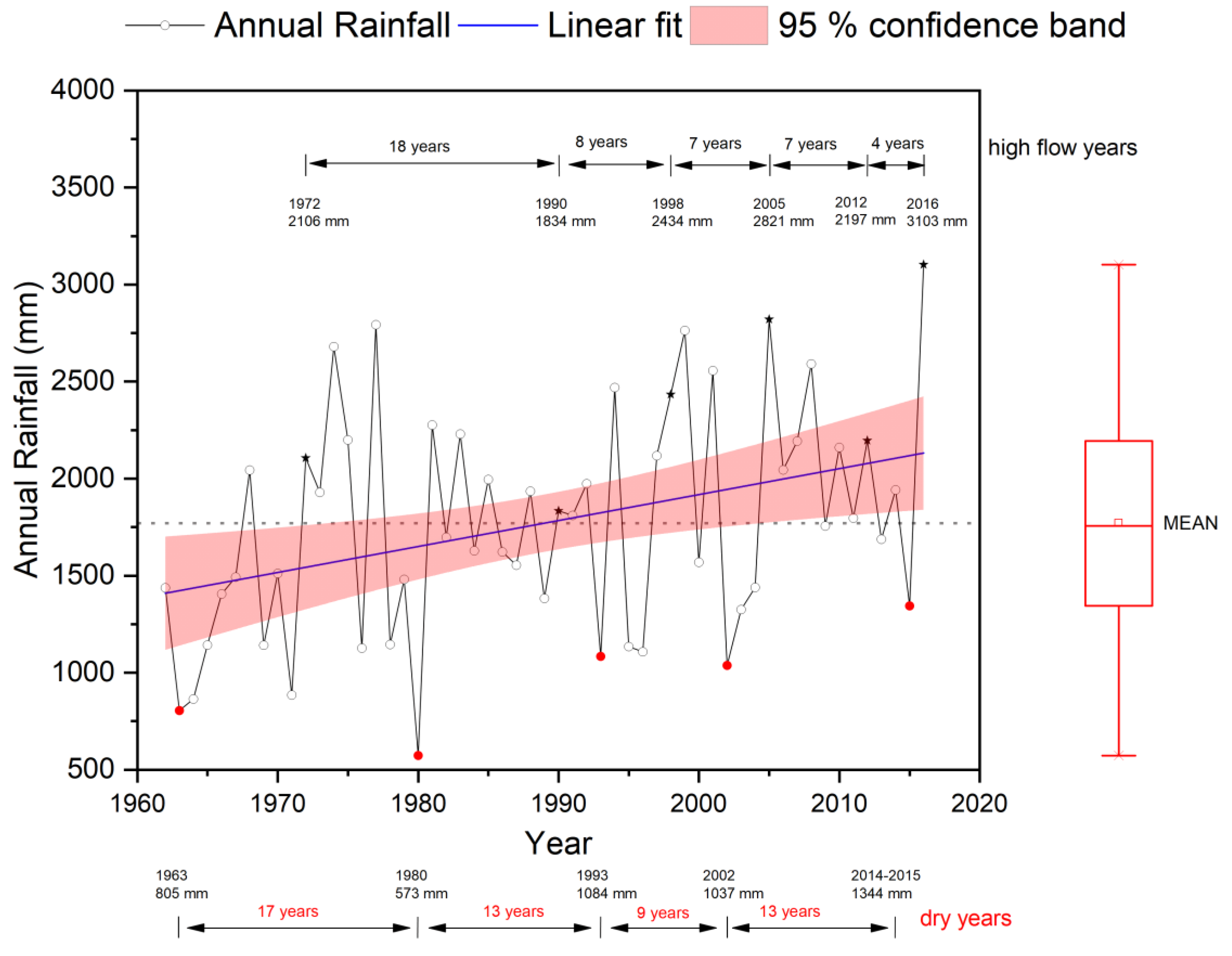
According to Taiwan’s hydrological data from the past 55 years, there has been a gradual increase in precipitation and typhoon intensity. Both the frequencies of occurrence and the severity of flooding are showing an increasing trend. Figure 3 and Figure 4 show the long-term climate and hydrological data from 1962 to 2016 recorded by the Kaohsiung weather station in the study area. From Figure 3, the annual average temperature in the study area exhibited an increasing trend. Beginning in 1997, the annual average temperature was higher than the average temperature in the past 55 years (24.8 °C) and after 2000, the increase of annual average temperature was more significant. Precipitation after 1996 was more significant and most of the annual precipitation was higher than the long-term annual average precipitation of 1770 mm. The deviation between high and low precipitation became larger and the duration of high and low precipitation became shorter (Figure 4).
2.3. The Physiographic Soil Erosion-Deposition Model (PSED Model)
The PSED Model [4,25] is a physical mechanism-based model that was developed by integrating the Geographic Information System (GIS) with a Physiographic Precipitation-Runoff model. It incorporates the effects of slope and river channel erosion, entrainment and deposition on river bed erosion-deposition for a watershed. Based on topography, landform, river system, land use and soil characteristics of the watershed, the PSED Model utilizes GIS to partition the watershed area into non-structural computational cells. The computed cells are then classified into slope cells, river cells and special cells. Esri ArcMap 10.7 was utilized to obtain hydrological and physiographical data within each cell. In addition, the extension modules of ArcMap (spatial analysis, hydrologic model, 3D Analyst and Network Analyst) and their object-oriented programming language were used.
The model consists mainly of two parts; a water flow simulation and a soil erosion-deposition simulation. Water flow simulation calculates the transport of precipitation runoff in the watershed area. The continuity equation of water flow is as follows:
where: t is time; Ai is area of the i cell; hi and hk represent the water stage of the i and k cell, respectively; Qi,k denotes the flow rate (discharge) from the k cell into its neighboring i cell; and Pei expresses the effective rainfall volume per second in the i cell, which is equal to the effective rainfall per second in the i cell multiplied by its area. Depending on the topography and landform information, the watershed area can be divided into several computed cells and the water level change of each cell should then satisfy the continuity equation of water flow and flow rate simulation, as expressed in Equation (1).
In the soil erosion-deposition simulation for the watershed, simulations for slope cells and river cells were calculated separately. The sediment transport rate and river bed erosion profile of each cell were simulated by using the suspended load equation (Equation (2)), the river bed variation continuity equations (Equation (3)) [26], and the river bed load transport equation.
where: Vsi is the soil volume of water body in i cell (= Ai × Di × Ci); D is the cell water depth; C is the suspended load volume concentration; is the porosity; Vdi is the alluvium volume of cell i; and denote the suspended and the river bed load flow rates, respectively, from the k cell into its neighboring i cell; represents the entrainment rate of ground surface soil or river bed sediment of the i-th cell; expresses the deposition rate of river bed sediment for i cell; and is the precipitation separation rate of the i cell.
2.4. Computational Cells
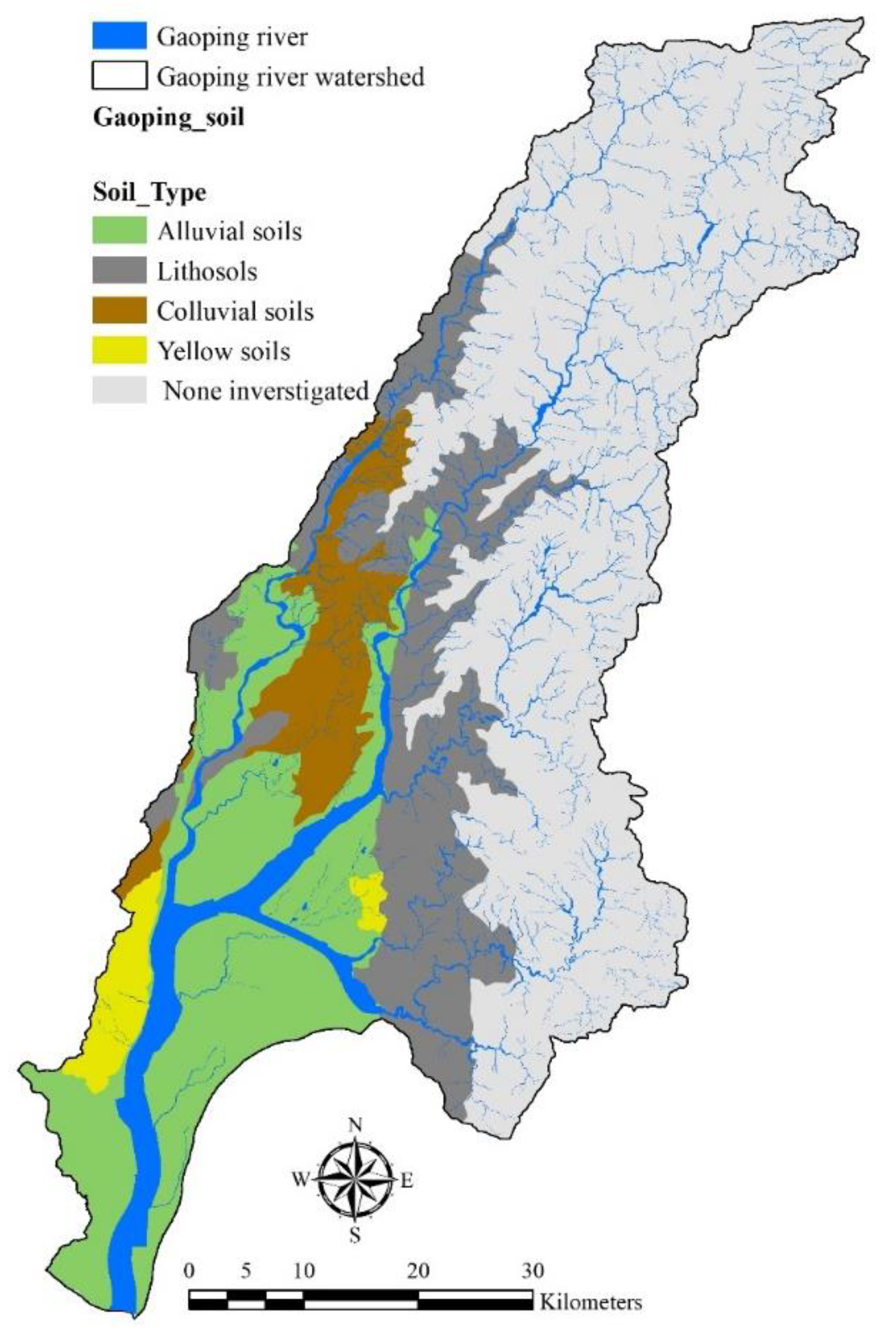
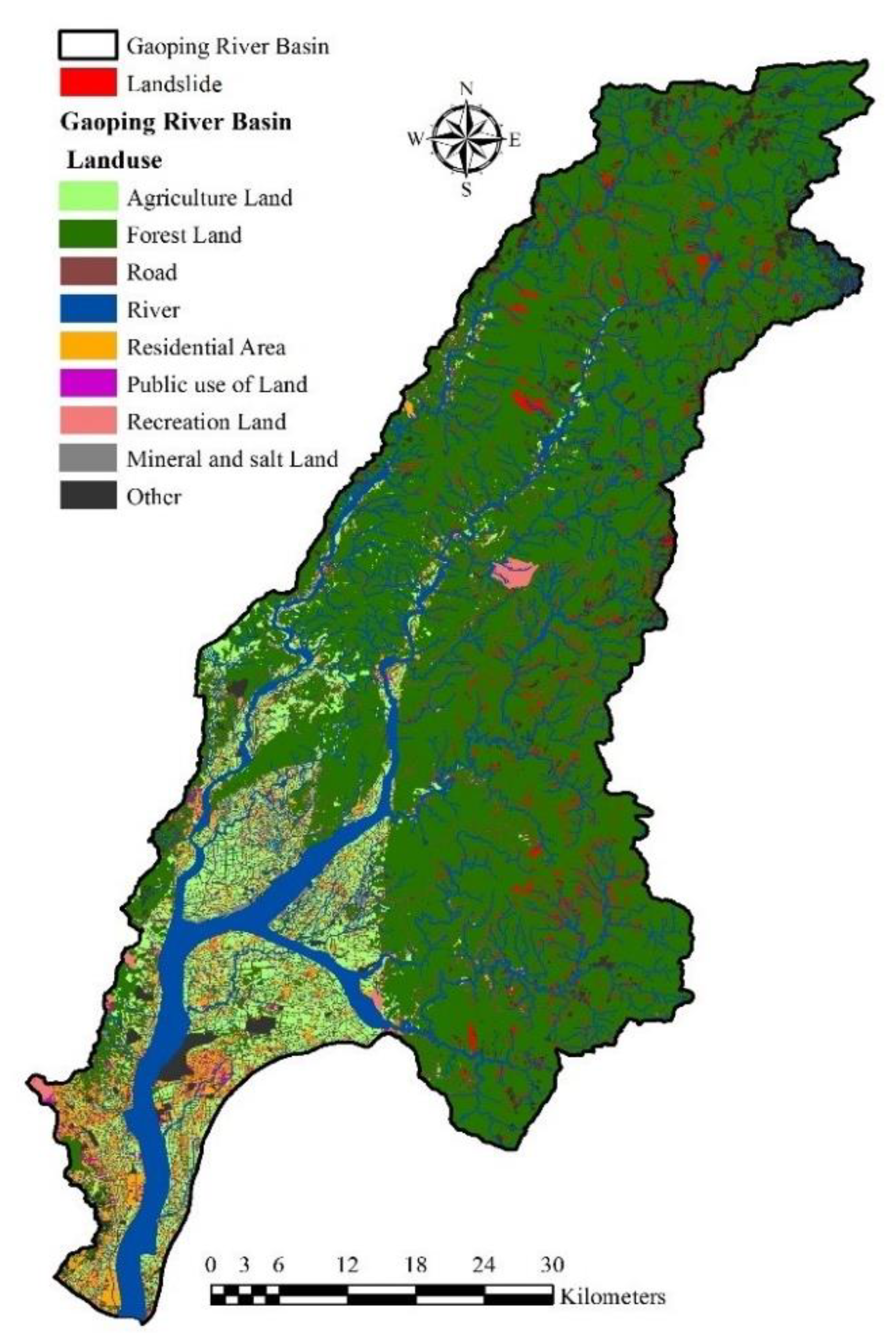
Figure 5, Figure 6 and Figure 7 show the Digital Elevation Model (DEM), soil map and land use maps of Gaoping River Basin, respectively. The basin ranges from 0 m to more than 3000 m above sea level and is dominated mostly by forest land at elevations higher than 500 m. Based on the DEM, land use, soil maps, road system maps, and slope maps (Figure 8) the basin was divided by Esri ArcMap 10.7 into 17,635 computational cells for further analysis.
2.5. Input Data and Model Setup
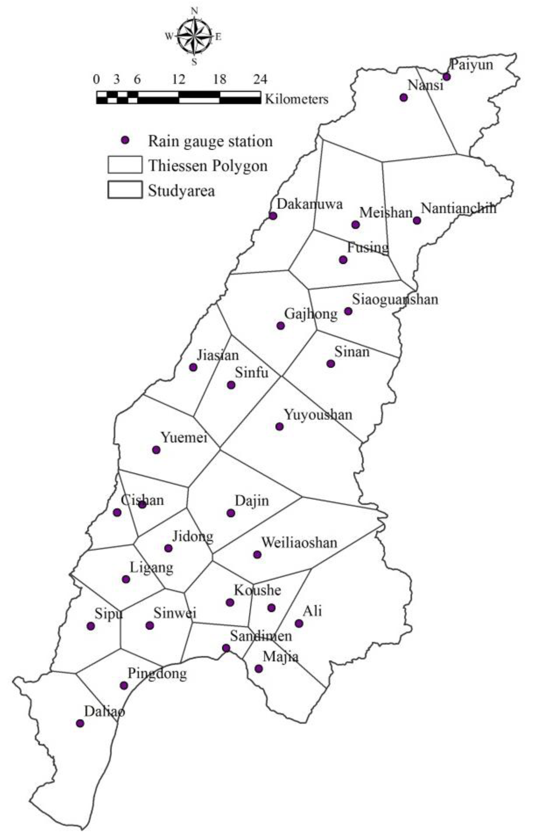
In the basin, there are 28 precipitation monitoring stations established by the Central Weather Bureau; however, they are not evenly distributed. In order to minimize computational errors, we applied the Thiessen polygons method to determine the controlling area of each precipitation monitoring station. The reader should note that the Thiessen polygons were not used to derive the weighted precipitation. Instead, precipitation data for each station were used as the precipitation volume of computed cells in the control area for the same precipitation monitoring station (Figure 9).
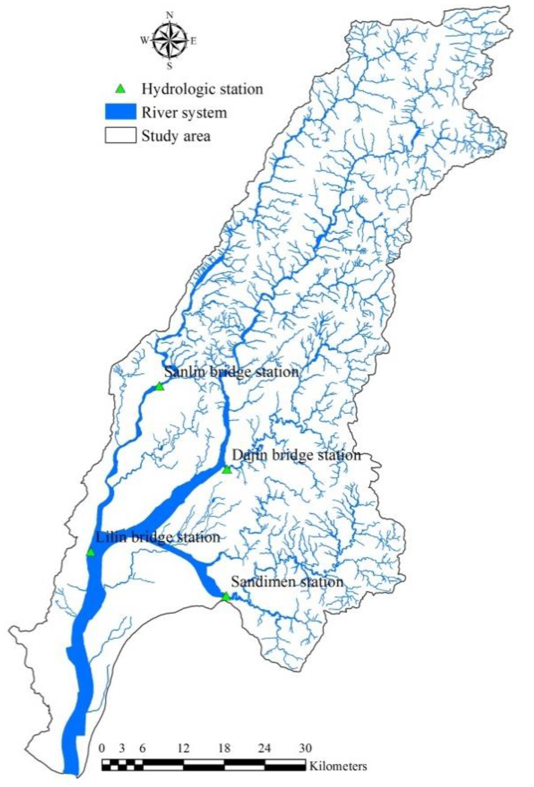
PSED simulated sediment transport was validated by comparing the flow rate and sediment transport data collected by sediment monitoring stations of the 7th River Management Office of Water Resources Agency, MOEA, which are located at the downstream of the Gaoping River and its tributaries. They include the Shanlin Bridge of Qishan River, Tachin Bridge of Laonong River, Sandimen Bridge of Ailiao River, and Lilin Bridge of Gaoping River (Figure 10).
The future scenario in this study was set from 2020 to 2039 and the corresponding baseline was set from 1980 to 1999. The Taiwan Climate Change Projection and Information Platform Project (TCCIP) provided downscaled precipitation data at 5 km2 resolution. To process the data, TCCIP relies on 24 GCMs as described in the Intergovernmental Panel on Climate Change (IPCC), Fourth Assessment Report (AR4) [29]. Additionally, IPCC identifies A2, A1B and B1 as the most probable scenarios; hence, this study adopted the A1B-S for analysis, which is regarded as a worse scenario and is similar to the A1B scenario. The worst-case scenario is primarily obtained through subtracting or adding one standard deviation between the estimated values of GCMs from the multi-model ensemble of all GCMs [30]. Monthly precipitation scenario information was further combined with a weather generator to evaluate the impact of climate change on daily precipitation volume.
The baseline was defined by precipitation data from 1980 to 1999. Historical daily precipitation data from the monitoring stations were used as input files for the climate derived models. These were then applied to generate the daily precipitation data representing the future climate change scenario. In addition, the daily precipitation data of the baseline scenario were combined with the precipitation distribution in the watershed area to translate into precipitation profiles to be used by the PSED model.
2.6. Model Verification
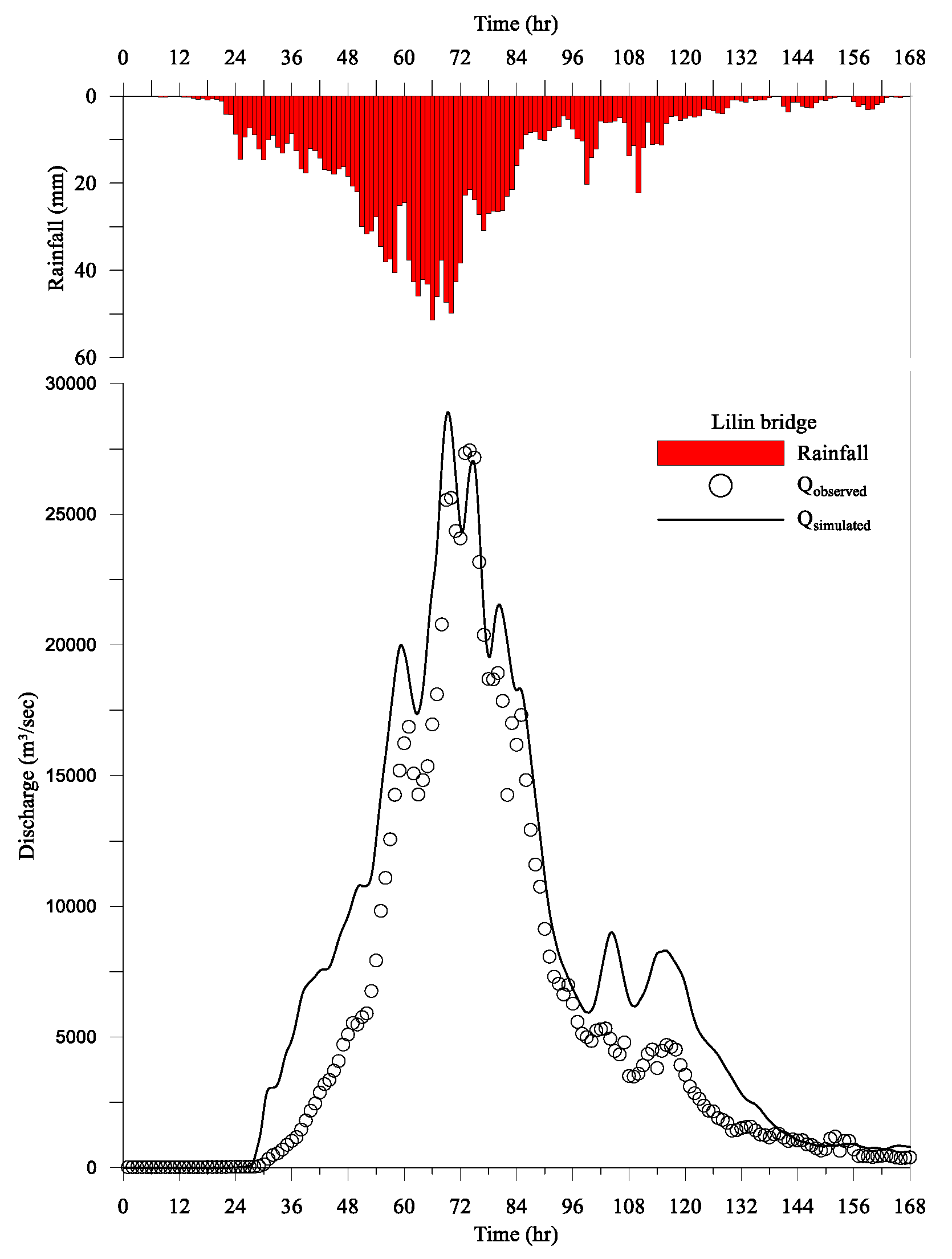
Typhoon Morakot (2009), the most disastrous storm to have hit Taiwan in the last century, was used to validate runoff and suspended load hydrographs from the PSED model. We further compared actual discharge and sediment transport from each hydrological station to simulated data. Simulated and observed flow hydrograph from Lilin Bridge is shown in Figure 11. The peak of the simulated hydrograph coincided with that from the observed data, and the hydrograph shapes are similar. This suggests that the model can be successfully applied.
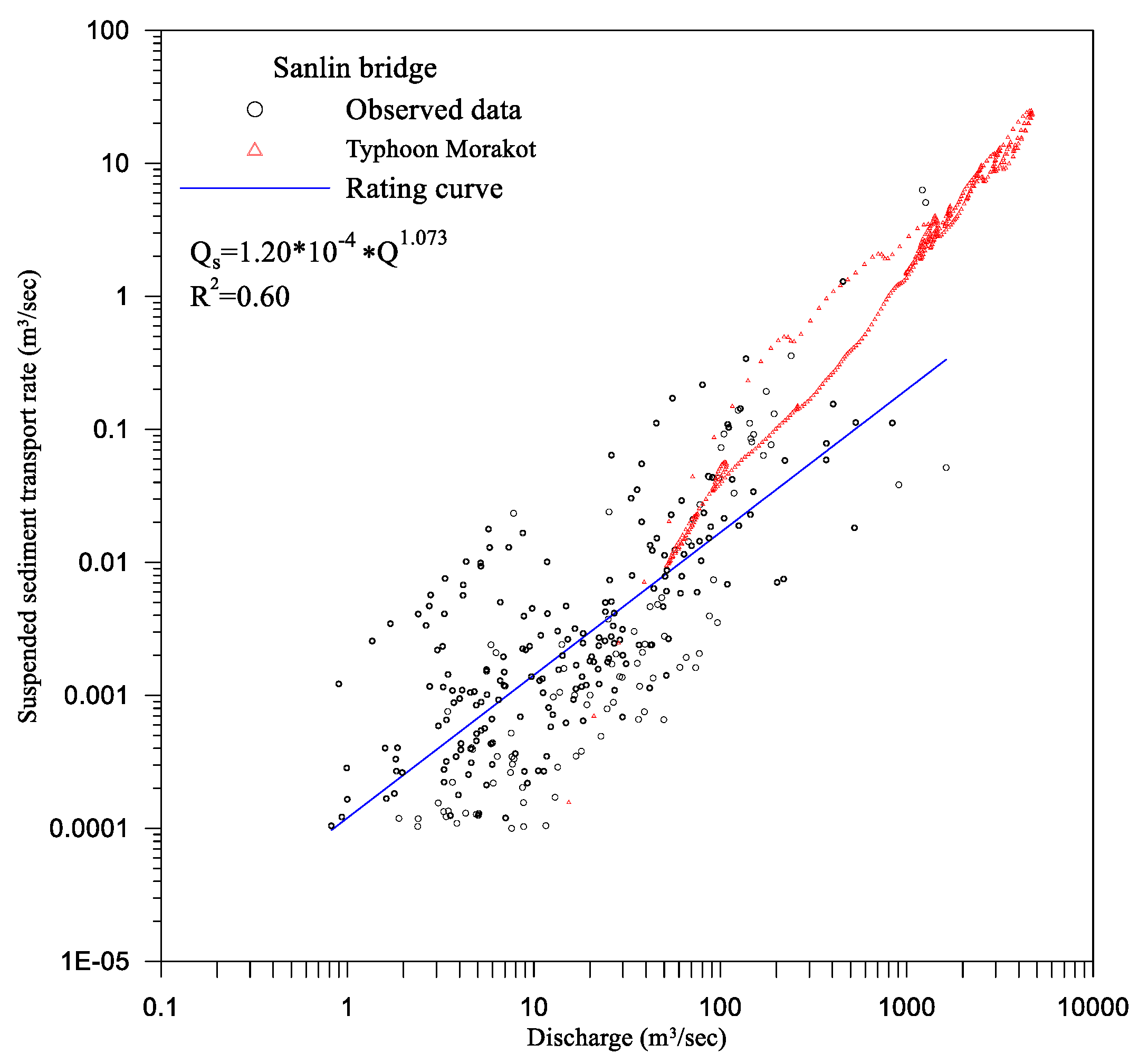
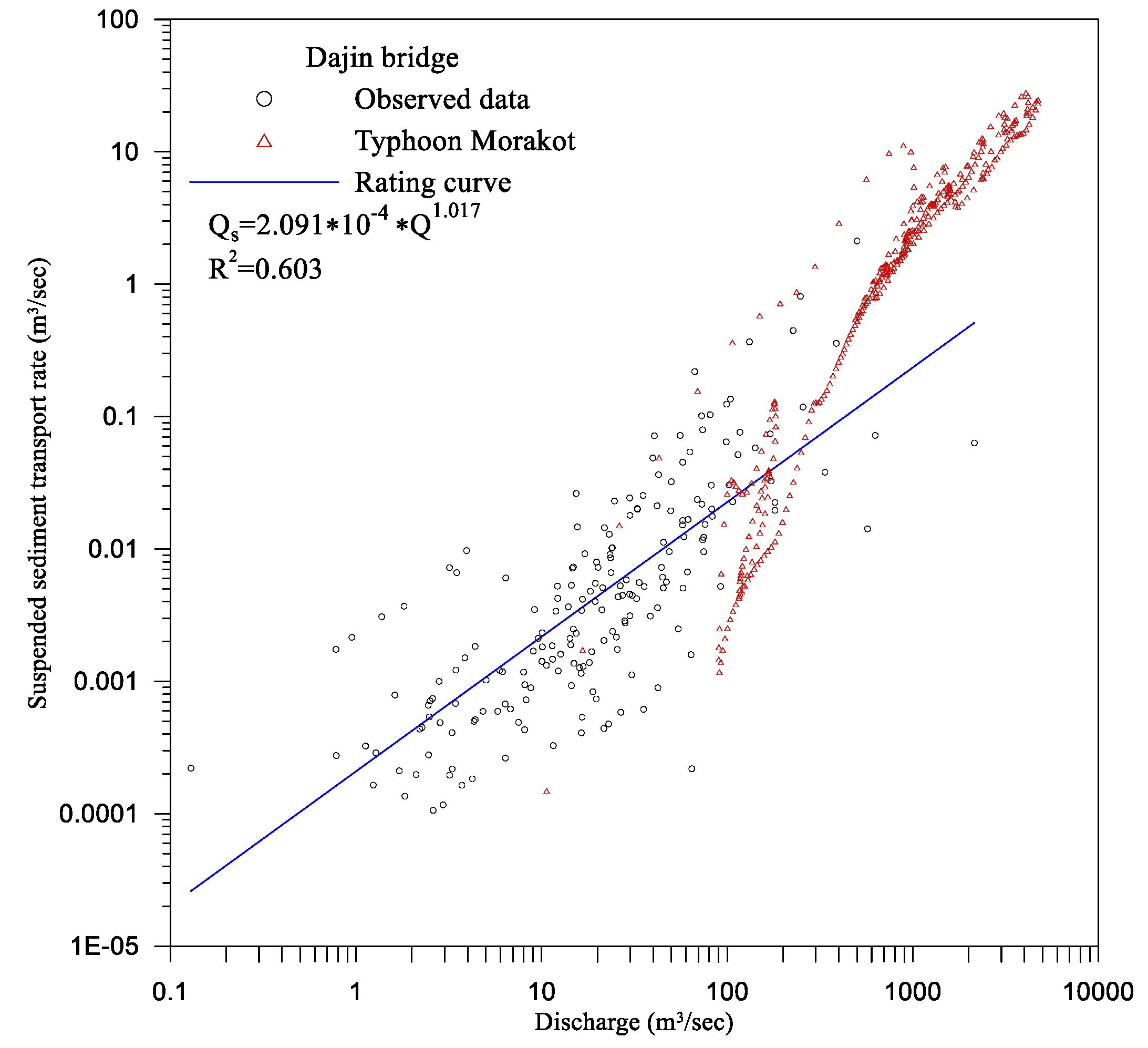
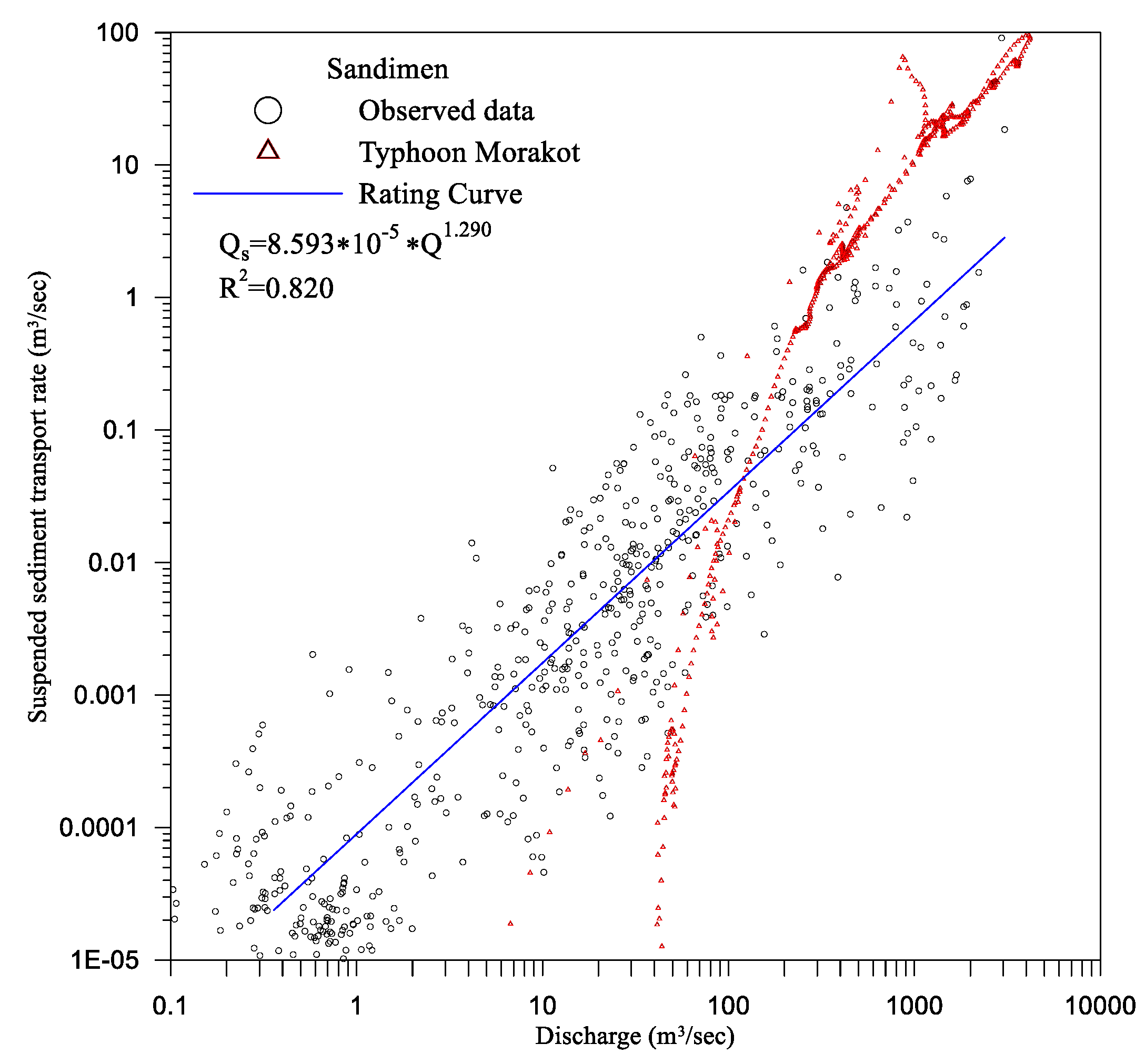
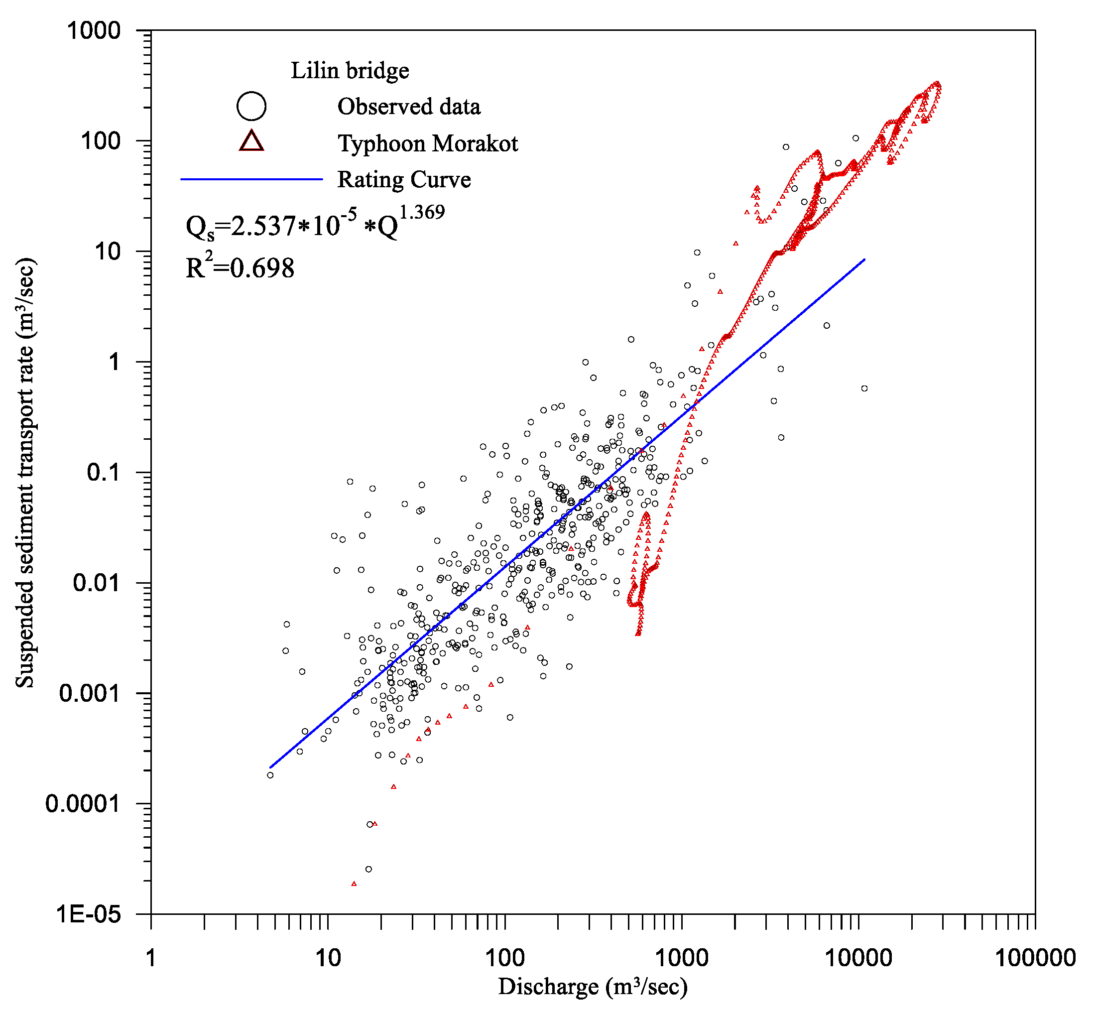
Since the hydrological monitoring stations along the Gaoping River system do not have suspended load concentration data hydrographs, the historical discharge and suspended load data from sediment monitoring stations downstream of the main branch of the Gaoping River were used to establish the correlation between discharge and sediment transport volume of each hydrological monitoring station. These served as the basis for validating the suspended load concentration hydrograph obtained from the numerical model. The simulated discharge and suspended load transport rate under Typhoon Morakot in 2009 were plotted onto the correlation diagram between the observed discharge and sediment transport rate for the Sanlin, Dajin, Sandimen and Lilin bridge Stations (Figure 12, Figure 13, Figure 14 and Figure 15). In these figures, points are actual historical measured data. The solid line represents the regression relation between discharge and sediment transport rate for each hydrological monitoring station. It is noted from the figures that the simulated correlation between discharge and sediment transport rate was consistent with the correlation between discharge and sediment transport rate of the actually observed data for all monitoring stations except Lilin Bridge station, particularly under high discharge. The model slightly overestimated data at this station (Figure 15). Nonetheless, the model also indicated reasonable estimates on suspended load and suspended load transport.
3. Results
3.1. Impacts of Climate Change on Erosion Volume and Sediment Yield
Different precipitation types, rainfall distribution, rainfall intensities and precipitation volume will result in different runoff processes, leading to different erosion volumes and sediment yields in a watershed. The precipitation volumes collected by each precipitation monitoring station in the watershed area for each return period (2, 5, 10, 25, 50, 100 and 200 year return period) under the baseline and A1B-S scenarios were used to calculate the average maximum rainfall intensity and average rainfall for each return period via the controlled area weighted method. The above return periods were selected as they are the standards used for most engineering designs in Taiwan. The precipitation results for the baseline were then compared with the results of the A1B-S scenario. Table 1 shows the comparison of average maximum rainfall intensity and average rainfall between the baseline and selected scenarios of each return period. Average maximum rainfall intensity increased more than average rainfall, suggesting that under the influence of climate change, not only did the precipitation volume increase but also the precipitation intensity.
Simulated erosion volume and sediment yield under the baseline and A1B-S scenarios for various return periods are shown in Table 2. Total erosion volume and sediment yield under the A1B-S scenario for various return periods are greater than under the baseline. The increase in the total sediment yield rate was higher than that of the total erosion volume. The total erosion volume and total sediment yield increases by 4–25% and 8–65%, respectively, when compared to the baseline. This implies that climate change contributed to 15% and 36% increases in soil erosion volume and sediment yield, respectively, when compared to the baseline average.
3.2. Climate Change Effect on Erosion and Erosion Distribution
Soil erosion simulation results for the studied area were compiled and summarized in Table 3. The least return period indicated a 0.54% increase in area, while for under 200 year return period there was a 2.3% increase. The impacts of climate change on erosion were found to be lower when compared to other areas within the Asian region. Pal and Chakrabortty [31] simulated the impacts of climate change on soil erosion in a sub-tropical monsoon dominated watershed based on a RUSLE model, and found erosion to increase by 33% under a 15 year return period.
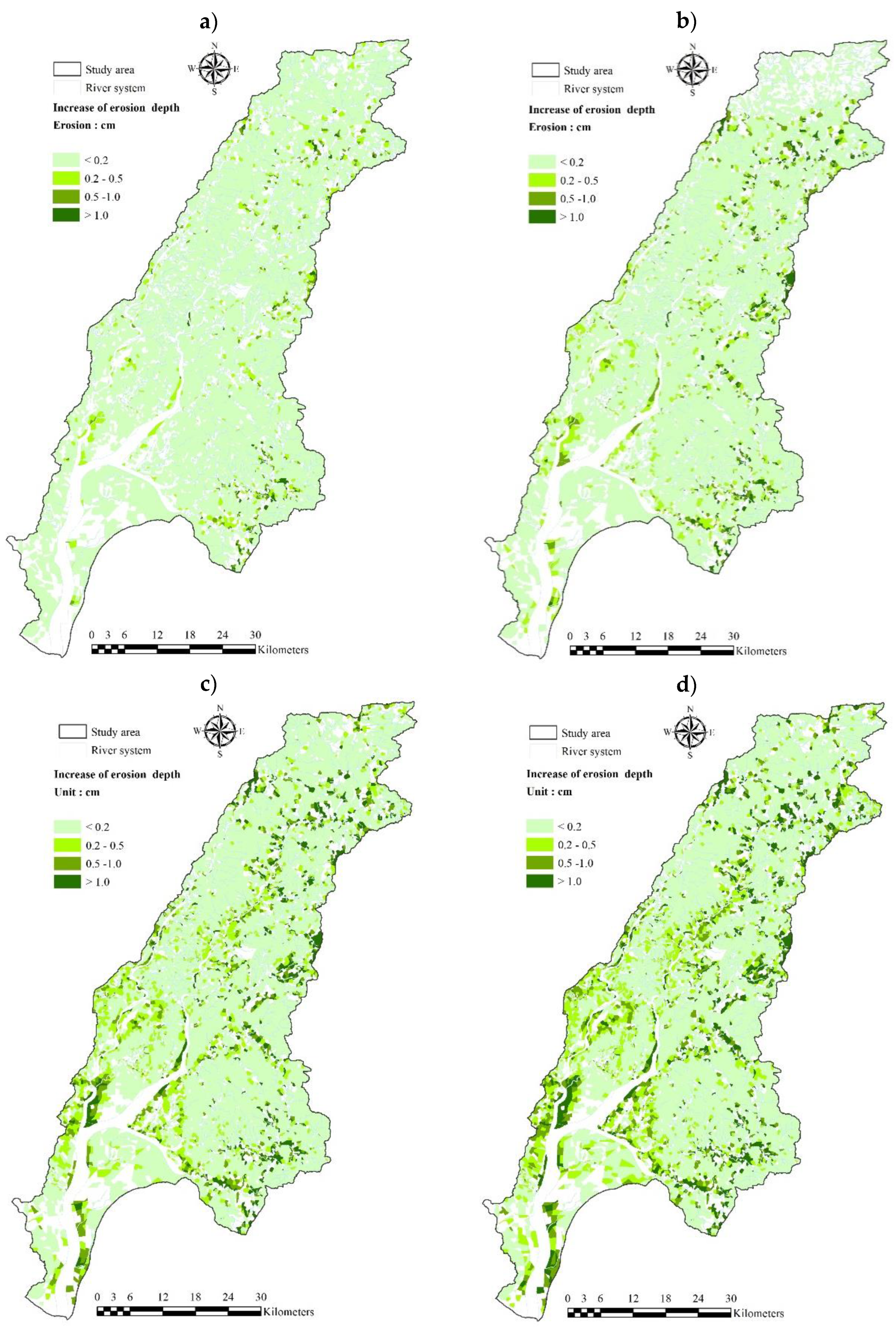
Climate change was also shown to cause larger erosion depths (Figure 16). Except in a few selected areas, a greater percentage indicates an increasing trend, and erosion depth increased with increasing return period. This is in line with observations made by Giang et al. [32], who predicted that Asian countries would be among the hardest hit regions globally.
3.3. Climate Change Effects on Deposition Volume and the Deposition Distribution
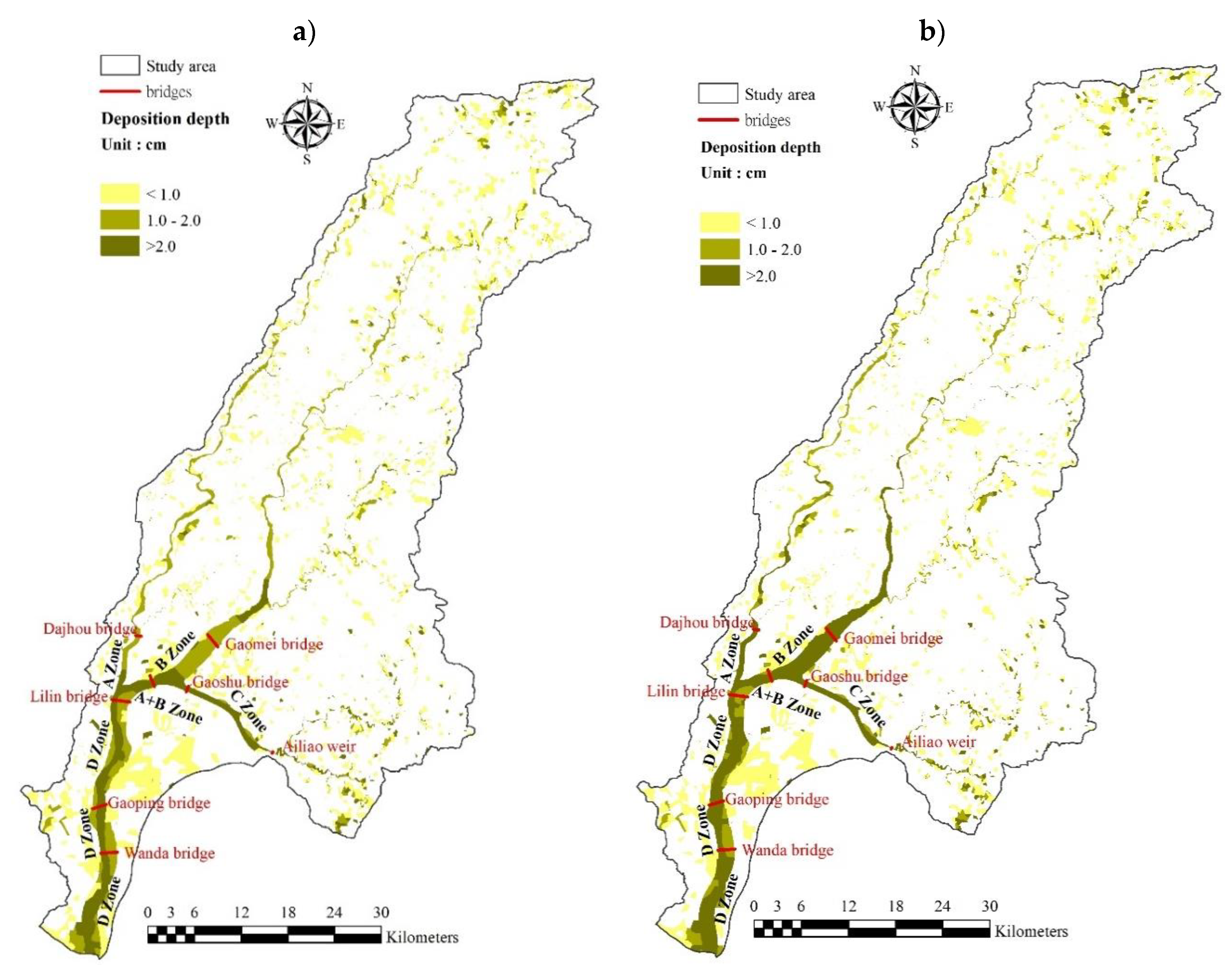
Deposition distributions under baseline and climate change scenarios for 10 and 100 year return periods are shown in Figure 17 and Figure 18, respectively. High deposition was observed mainly at the confluences; between Gaoping and Qishan River (zone A), Gaoping River and Laonong River (zone B), Ailiao River Gaoshu Bridge and Ailiao weir (zone C) and in the middle and downstream of Gaoping River (zone D). Zone areas are shown in Figure 19. Large deposition at these areas is attributed to widening of the cross sections, low river bed slopes and low flow rates. Deposition in each computational cell was calculated by multiplying the deposition height of a cell by its area, and the total deposition of all cells was simply the summation of the volumes in each cell. A summary of the deposition under the different return periods is shown in Table 4.
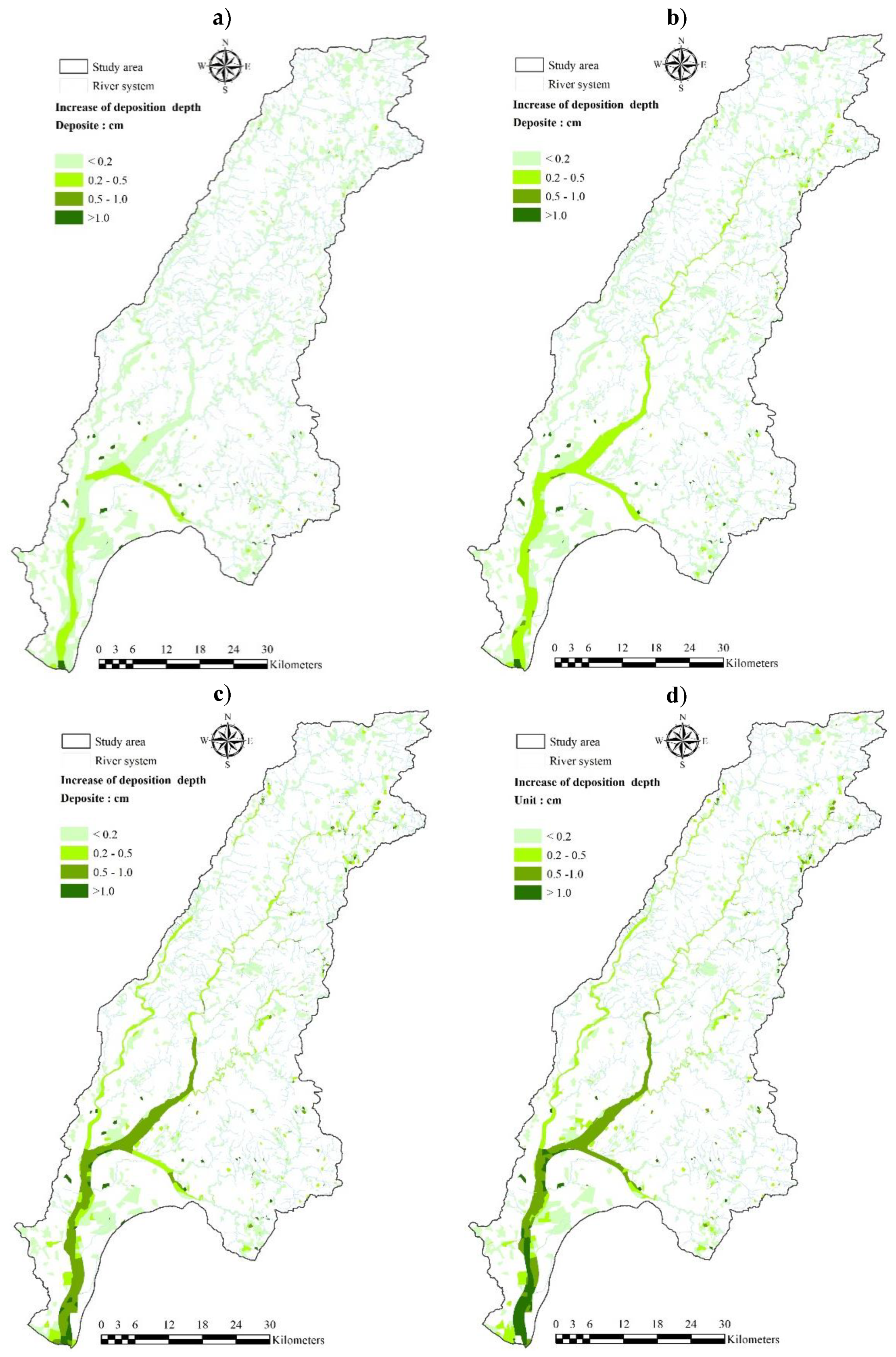
Figure 20 shows the spatial distribution of deposition depth increase under the baseline and climate change scenarios. Similar increase patterns were observed between the simulated cases, with a larger deposition depth increase located in the middle and downstream of river channels. Deposition depth increase was highest in the main channel as expected, and increased with increasing return periods indicated by dark green areas in Figure 20.
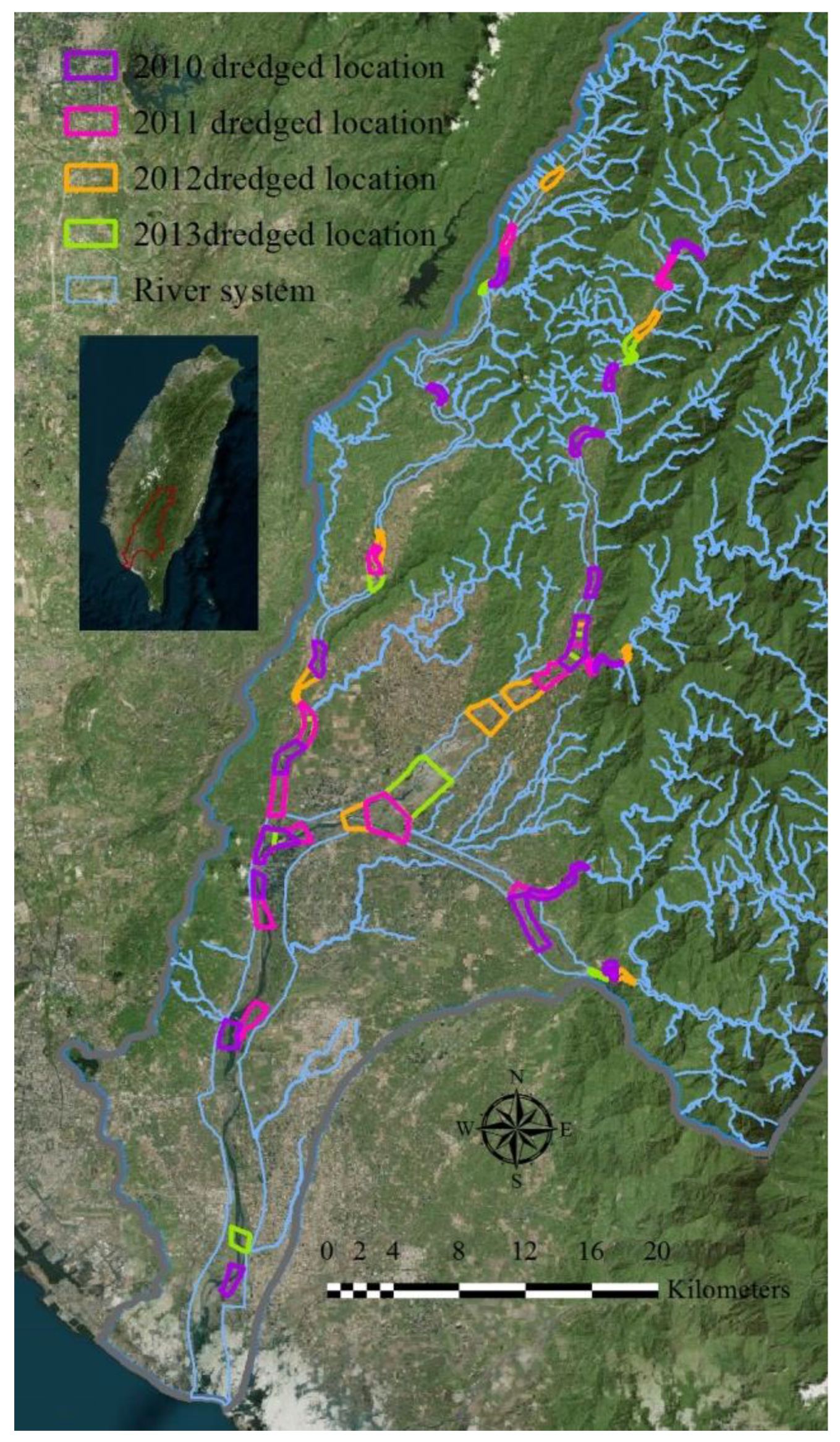
Gaoping River basin exhibited high erosion volume and sediment yield. According to statistical data reported by the Water Resources Agency [22], 76,870,000 m3 have been dredged between 2010 and 2013. Table 5 shows the dredged volume of each year, while Figure 21 indicates the location of the dredged site. Dredged locations coincide with high deposition areas computed by the PSED model, as illustrated by Figure 21.
In each year, a huge amount of money is needed to carry out the dredging works at Gaoping River. With climate change increasing the deposition rates, not only will there be more pressure on financial resources, but flooding risk is also expected to increase. Hence, appropriate structures and policies should be put in place in order to redress climate change impacts. Proposed strategies include identifying and mapping areas more prone to soil erosion and implementing river management and stability measures. Planning the overall river basin operations and management strategies can effectively control the sediment yield in a watershed, hence reducing sediment deposition in river channels due to soil erosion and eliminating flooding disasters due to limited water passage.
4. Conclusions
This study applied a numerical model to investigate the impacts of climate change on erosion volume, sediment yield and erosion deposition in a watershed. The results showed that precipitation under the A1B-S climate change scenario would significantly increase soil erosion volume, sediment yield and sediment transport rate. Total erosion volume and total sediment yield in the watershed under the A1B-S scenario for various return periods increased by 4–25% and 8–65%, respectively, from 2 year to 200 year return periods. Climate change further increased deposition volume by 2–23% relative to the baseline and by 13% relative to the baseline average. Deposition was found to mostly occur at the river confluences, river middle and at the downstream end of Gaoping River. The study clearly revealed the adverse impacts climate change is likely to bring to this basin; hence, appropriate conservation measures are suggested.
Author Contributions
Conceptualization, methodology, formal analysis, C.-N.C.; data curation, C.-H.T.; validation, writing—review and editing, S.S.T. All authors have read and agreed to the published version of the manuscript.
Funding
This research was funded by the Ministry of Science and Technology (MOST) of Taiwan, grant number MOST-107-2221E-020-006.
Acknowledgments
The authors extend their gratitude toward the anonymous reviewers for their valuable comments to improve the quality of the manuscript.
Conflicts of Interest
The authors declare no conflict of interest.
References
- Diodato, N.; Filizola, N.; Borrelli, P.; Panagos, P.; Bellocchi, G. The Rise of Climate-Driven Sediment Discharge in the Amazonian River Basin. Atmosphere 2020, 11, 208. [Google Scholar] [CrossRef] [Green Version]
- Babur, M.; Shrestha, S.; Bhatta, B.; Datta, A.; Ullah, H. Integrated Assessment of Extreme Climate and Landuse Change Impact on Sediment Yield in a Mountainous Transboundary Watershed of India and Pakistan. J. Mt. Sci. 2020, 17, 624–640. [Google Scholar] [CrossRef]
- Gupta, S.; Kumar, S. Simulating Climate Change Impact on Soil Erosion Using Rusle Model—A Case Study in a Watershed of Mid-Himalayan Landscape. J. Earth Syst. Sci. 2017, 126, 43. [Google Scholar] [CrossRef]
- Chen, C.-N.; Tsai, C.-H.; Tsai, C.-T. Simulation of Sediment Yield from Watershed by Physiographic Soil Erosion–Deposition Model. J. Hydrol. 2006, 327, 293–303. [Google Scholar] [CrossRef]
- Wang, H.-W.; Kondolf, M.; Tullos, D.; Kuo, W.-C. Sediment Management in Taiwan’s Reservoirs and Barriers to Implementation. Water 2018, 10, 1034. [Google Scholar] [CrossRef] [Green Version]
- Stefanidis, S.; Stathis, D. Effect of Climate Change on Soil Erosion in a Mountainous Mediterranean Catchment (Central Pindus, Greece). Water 2018, 10, 1469. [Google Scholar] [CrossRef] [Green Version]
- Jha, M. Impacts of Climate Change on Streamflow in the Upper Mississippi River Basin: A Regional Climate Model Perspective. J. Geophys. Res. 2004, 109, 1–12. [Google Scholar] [CrossRef]
- Abbaspour, K.C.; Faramarzi, M.; Ghasemi, S.S.; Yang, H. Assessing the Impact of Climate Change on Water Resources in Iran. Water Resour. Res. 2009, 45, 1–16. [Google Scholar] [CrossRef] [Green Version]
- Zhang, R.; Corte-Real, J.; Moreira, M.; Kilsby, C.; Birkinshaw, S.; Burton, A.; Fowler, H.J.; Forsythe, N.; Nunes, J.P.; Sampaio, E.; et al. Downscaling Climate Change of Water Availability, Sediment Yield and Extreme Events: Application to a Mediterranean Climate Basin. Int. J. Climatol. 2019, 39, 2947–2963. [Google Scholar] [CrossRef]
- Chang, T.J.; Hsu, M.H.; Lin, G.F.; Lai, J.S.; Pan, T.Y. Investigation on Analysis Method of Flood Vulnerability and Risk; Water Resources Agency: Taipei, Taiwan, 2010.
- Zarghami, M.; Abdi, A.; Babaeian, I.; Hassanzadeh, Y.; Kanani, R. Impacts of Climate Change on Runoffs in East Azerbaijan, Iran. Glob. Planet. Chang. 2011, 78, 137–146. [Google Scholar] [CrossRef]
- Kumar, N.; Tischbein, B.; Kusche, J.; Laux, P.; Beg, M.K.; Bogardi, J.J. Impact of Climate Change on Water Resources of Upper Kharun Catchment in Chhattisgarh, India. J. Hydrol. Reg. Stud. 2017, 13, 189–207. [Google Scholar] [CrossRef]
- Leta, O.T.; El-Kadi, A.I.; Dulai, H.; Ghazal, K.A. Assessment of Climate Change Impacts on Water Balance Components of Heeia Watershed in Hawaii. J. Hydrol. Reg. Stud. 2016, 8, 182–197. [Google Scholar] [CrossRef] [Green Version]
- Thodsen, H.; Hasholt, B.; Kjærsgaard, J.H. The Influence of Climate Change on Suspended Sediment Transport in Danish Rivers. Hydrol. Process. 2008, 22, 764–774. [Google Scholar] [CrossRef]
- Phan, D.B.; Wu, C.C.; Hsieh, S.C. Impact of Climate Change on Stream Discharge and Sediment Yield in Northern Viet Nam. Water Resour. 2011, 38, 827–836. [Google Scholar] [CrossRef]
- Cousino, L.K.; Becker, R.H.; Zmijewski, K.A. Modeling the Effects of Climate Change on Water, Sediment, and Nutrient Yields from the Maumee River Watershed. J. Hydrol. Reg. Stud. 2015, 4, 762–775. [Google Scholar] [CrossRef]
- Zhou, Y.; Xu, Y.; Xiao, W.; Wang, J.; Huang, Y.; Yang, H. Climate Change Impacts on Flow and Suspended Sediment Yield in Headwaters of High-Latitude Regions—A Case Study in China’s Far Northeast. Water 2017, 9, 966. [Google Scholar] [CrossRef] [Green Version]
- Azari, M.; Moradi, H.R.; Saghafian, B.; Faramarzi, M. Climate Change Impacts on Streamflow and Sediment Yield in the North of Iran. Hydrol. Sci. J. 2016, 61, 123–133. [Google Scholar] [CrossRef]
- Zhang, S.; Li, Z.; Lin, X.; Zhang, C. Assessment of Climate Change and Associated Vegetation Cover Change on Watershed-Scale Runoff and Sediment Yield. Water 2019, 11, 1373. [Google Scholar] [CrossRef] [Green Version]
- Renard, K.G.; Foster, G.R.; Weesies, G.A.; Porter, J.P. Rusle: Revised Universal Soil Loss Equation. J. Soil Water Consv. 1991, 46, 30–33. [Google Scholar]
- Tfwala, S.; Wang, Y.-M. Estimating Sediment Discharge Using Sediment Rating Curves and Artificial Neural Networks in the Shiwen River, Taiwan. Water 2016, 8, 53. [Google Scholar] [CrossRef] [Green Version]
- Water Resources Agency. Assessment of the Efficiency of Dredging Engineering in the Kaoping River Watershed; Ministry of Economic Affairs: Taichung, Taiwan, 2014.
- Yu, S.-W.; Tsai, L.L.; Talling, P.J.; Lin, A.T.; Mii, H.-S.; Chung, S.-H.; Horng, C.-S. Sea Level and Climatic Controls on Turbidite Occurrence for the Past 26kyr on the Flank of the Gaoping Canyon Off Sw Taiwan. Mar. Geol. 2017, 392, 140–150. [Google Scholar] [CrossRef]
- Central Geological Survey. Geological Information Service; Affairs, M.O.E., Ed.; Central Geological Survey: Taipei, Taiwan, 2000.
- Chen, C.N.; Tsai, C.H.; Tsai, C.T. Simulation of Runoff and Suspended Sediment Transport Rate in a Basin with Multiple Watersheds. Water Resour. Manage. 2011, 25, 793–816. [Google Scholar] [CrossRef] [Green Version]
- Lin, C.-P.; Chen, C.-N.; Wang, Y.-M.; Tsai, C.-H.; Tsai, C.-T. Spatial Distribution of Soil Erosion and Suspended Sediment Transport Rate for Chou-Shui River Basin. J. Earth Syst. Sci. 2014, 123, 1517–1539. [Google Scholar] [CrossRef]
- Taiwan Agricultural Research Institute. Soil Maps of Taiwan; Council of Agriculture: Taichung, Taiwan, 2004.
- National Land Surveying and Mapping Center. Land Use Maps of Taiwan; Ministry of the Interior: Taichung, Taiwan, 2006.
- Intergovernmental Panel on Climate Change. Climate Change 2014: Synthesis Report; IPCC: Geneva, Switzerland, 2014; p. 151. [Google Scholar]
- Chen, C.-N.; Tfwala, S. Impacts of Climate Change and Land Subsidence on Inundation Risk. Water 2018, 10, 157. [Google Scholar] [CrossRef] [Green Version]
- Pal, S.C.; Chakrabortty, R. Simulating the Impact of Climate Change on Soil Erosion in Sub-Tropical Monsoon Dominated Watershed Based on Rusle, Scs Runoff and Miroc5 Climatic Model. Adv. Space Res. 2019, 64, 352–377. [Google Scholar] [CrossRef]
- Giang, P.Q.; Giang, L.T.; Toshiki, K. Spatial and Temporal Responses of Soil Erosion to Climate Change Impacts in a Transnational Watershed in Southeast Asia. Climate 2017, 5, 22. [Google Scholar] [CrossRef]
Figure 1.
The drainage network in the Gaoping River basin.

Figure 2.
Geological map of Gaoping watershed [24].
Figure 2.
Geological map of Gaoping watershed [24].

Figure 3.
Changes in annual average temperature recorded by the Kaohsiung weather station, 1960–2016.
Figure 3.
Changes in annual average temperature recorded by the Kaohsiung weather station, 1960–2016.

Figure 4.
Changes in annual precipitation recorded by the Kaohsiung Weather Station, 1960–2016.

Figure 5.
Digital elevation model (DEM) of the Gaoping River watershed.

Figure 6.
Soil map of the Gaoping River watershed [27].
Figure 6.
Soil map of the Gaoping River watershed [27].

Figure 7.
Digital land use map of the Gaoping River watershed [28].
Figure 7.
Digital land use map of the Gaoping River watershed [28].

Figure 8.
Slope map of Gaoping River watershed.

Figure 9.
Effective area for precipitation gauging stations in the Gaoping River watershed.

Figure 10.
Sediment monitoring stations on the Gaoping River and its tributaries.

Figure 11.
Simulated and observed discharge during Typhoon Morakot in 2009 at Lilin Bridge station.

Figure 12.
Simulated and observed correlation between flow discharge and sediment transport rate at Sanlin Bridge station.
Figure 12.
Simulated and observed correlation between flow discharge and sediment transport rate at Sanlin Bridge station.

Figure 13.
Simulated and observed correlation between flow discharge and sediment transport rate at Dajin Bridge station.
Figure 13.
Simulated and observed correlation between flow discharge and sediment transport rate at Dajin Bridge station.

Figure 14.
Simulated and observed relationship between flow discharge and sediment transport rate at Sandimen Bridge station.
Figure 14.
Simulated and observed relationship between flow discharge and sediment transport rate at Sandimen Bridge station.

Figure 15.
Simulated and observed relationship between flow discharge and sediment transport rate at Lilin Bridge station.
Figure 15.
Simulated and observed relationship between flow discharge and sediment transport rate at Lilin Bridge station.

Figure 16.
Spatial distribution of erosion depth increase under the influence of climate change under (a) 10 year, (b) 25 year, (c) 100 year and (d) 200 year return periods.
Figure 16.
Spatial distribution of erosion depth increase under the influence of climate change under (a) 10 year, (b) 25 year, (c) 100 year and (d) 200 year return periods.

Figure 17.
Deposition depth distribution under 10 year return period for (a) baseline and (b) climate change scenarios.
Figure 17.
Deposition depth distribution under 10 year return period for (a) baseline and (b) climate change scenarios.

Figure 18.
Deposition depth distribution under 100 year return period for (a) baseline and (b) climate change scenarios.
Figure 18.
Deposition depth distribution under 100 year return period for (a) baseline and (b) climate change scenarios.

Figure 19.
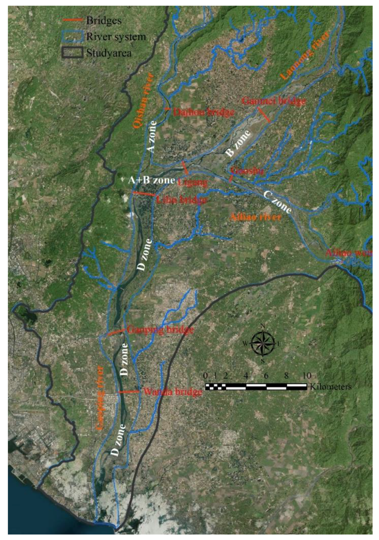
Location of various river sections in the Gaoping River basin that are vulnerable to soil deposition.
Figure 19.
Location of various river sections in the Gaoping River basin that are vulnerable to soil deposition.

Figure 20.
Spatial distribution of deposition depth increase under the influence of climate change for (a) 10 year, (b) 25 year, (c) 100 year and (d) 200 year return periods.
Figure 20.
Spatial distribution of deposition depth increase under the influence of climate change for (a) 10 year, (b) 25 year, (c) 100 year and (d) 200 year return periods.

Figure 21.
Dredged locations in Gaoping River basin from 2010 to 2013.


Table 1.
Average maximum rainfall intensity and average rainfall increase rates under baseline and A1B-S scenarios for various return periods.
Table 1.
Average maximum rainfall intensity and average rainfall increase rates under baseline and A1B-S scenarios for various return periods.
| Return Period | Average Maximum Rainfall Intensity (mm/hr) | Average Annual Rainfall (mm) | ||||
|---|---|---|---|---|---|---|
| Baseline (1980–1999) | A1B-S (2020–2039) | Increase Rate (%) | Baseline (1980–1999) | A1B-S (2020–2039) | Increase Rate (%) | |
| 2 | 27.52 | 29.14 | 5.89 | 411.18 | 434.90 | 5.77 |
| 5 | 39.00 | 41.90 | 7.43 | 584.82 | 627.39 | 7.28 |
| 10 | 46.53 | 51.63 | 10.97 | 701.12 | 776.94 | 10.81 |
| 25 | 55.10 | 65.92 | 19.65 | 843.42 | 1004.26 | 19.07 |
| 50 | 61.12 | 78.24 | 27.99 | 957.97 | 1212.17 | 26.53 |
| 100 | 66.96 | 91.98 | 37.36 | 1094.72 | 1466.32 | 33.95 |
| 200 | 72.75 | 107.35 | 47.56 | 1280.60 | 1794.54 | 40.13 |
Table 2.
Soil erosion and sediment yield increase rates under baseline and A1B-S scenarios for various return periods.
Table 2.
Soil erosion and sediment yield increase rates under baseline and A1B-S scenarios for various return periods.
| Return Period | Total Erosion (m3) | Total Sediment Yield (m3) | ||||
|---|---|---|---|---|---|---|
| Baseline (1980–1999) | A1B-S (2020–2039) | Increase Rate (%) | Baseline (1980–1999) | A1B-S (2020–2039) | Increase Rate (%) | |
| 2 | 25,025,101 | 26,158,002 | 4.53 | 3,610,538 | 3,919,368 | 8.55 |
| 5 | 33,683,874 | 35,566,538 | 5.59 | 6,312,775 | 7,083,252 | 12.21 |
| 10 | 38,589,952 | 41,576,563 | 7.74 | 8,280,890 | 9,711,170 | 17.27 |
| 25 | 43,557,305 | 49,077,034 | 12.67 | 10,631,451 | 13,811,304 | 29.91 |
| 50 | 46,687,318 | 54,601,150 | 16.95 | 12,325,453 | 17,496,549 | 41.95 |
| 100 | 49,482,826 | 59,940,637 | 21.13 | 14,010,777 | 21,564,822 | 53.92 |
| 200 | 52,023,499 | 65,223,943 | 25.37 | 15,708,576 | 25,927,062 | 65.05 |
Table 3.
Comparison of the increase rate of soil erosion area increase under the baseline and A1B-S scenarios for various return periods.
Table 3.
Comparison of the increase rate of soil erosion area increase under the baseline and A1B-S scenarios for various return periods.
| Return Period | Area Increase (m2) | Increase Rate (%) |
|---|---|---|
| 2 | 11,888,256 | 0.54 |
| 5 | 16,749,128 | 0.7 |
| 10 | 29,890,573 | 1.22 |
| 25 | 42,155,931 | 1.67 |
| 50 | 47,859,021 | 1.92 |
| 100 | 50,239,407 | 1.97 |
| 200 | 58,921,624 | 2.3 |
Table 4.
Increase in volume of estimated sediment deposition under baseline (1980–1999) and A1B-S (2020–2039) scenarios for various return periods.
Table 4.
Increase in volume of estimated sediment deposition under baseline (1980–1999) and A1B-S (2020–2039) scenarios for various return periods.
| Return Period | Baseline (m3) (1980–1999) | A1B-S (m3) (2020–2039) | Deposition Volume Increase for Baseline and A1B-S Scenarios (m3) | Increase Rate (%) |
|---|---|---|---|---|
| 2 | 9,499,196 | 9,720,588 | 221,392 | 2.33 |
| 5 | 11,984,107 | 12,425,532 | 441,425 | 3.68 |
| 10 | 13,292,933 | 14,141,714 | 848,781 | 6.39 |
| 25 | 14,618,375 | 16,252,862 | 1,634,487 | 11.18 |
| 50 | 15,424,874 | 17,836,223 | 2,411,349 | 15.63 |
| 100 | 16,180,722 | 19,313,894 | 3,133,172 | 19.36 |
| 200 | 16,855,567 | 20,857,945 | 4,002,378 | 23.75 |
Table 5.
The actual dredged sediment deposition amounts from 2010 to 2013 in each river [22].
Table 5.
The actual dredged sediment deposition amounts from 2010 to 2013 in each river [22].
| River | Actual Dredged Amount (104 m3) | |||
|---|---|---|---|---|
| 2010 | 2011 | 2012 | 2013 | |
| Laonong | 947.26 | 1516.37 | 855.74 | 623.36 |
| Zhuokou | 27.68 | 75.00 | 6.49 | 44.60 |
| Qishan | 423.07 | 241.70 | 187.77 | 244.46 |
| Ailiao | 555.21 | 689.79 | 184.91 | 139.99 |
| Gaoping | 534.61 | 203.68 | 104.33 | 81.54 |
| Total | 2487.83 | 2726.54 | 1339.24 | 1133.95 |
© 2020 by the authors. Licensee MDPI, Basel, Switzerland. This article is an open access article distributed under the terms and conditions of the Creative Commons Attribution (CC BY) license (http://creativecommons.org/licenses/by/4.0/).
Share and Cite
MDPI and ACS Style
Chen, C.-N.; Tfwala, S.S.; Tsai, C.-H. Climate Change Impacts on Soil Erosion and Sediment Yield in a Watershed. Water 2020, 12, 2247. https://0-doi-org.brum.beds.ac.uk/10.3390/w12082247
AMA Style
Chen C-N, Tfwala SS, Tsai C-H. Climate Change Impacts on Soil Erosion and Sediment Yield in a Watershed. Water. 2020; 12(8):2247. https://0-doi-org.brum.beds.ac.uk/10.3390/w12082247
Chicago/Turabian StyleChen, Ching-Nuo, Samkele S. Tfwala, and Chih-Heng Tsai. 2020. "Climate Change Impacts on Soil Erosion and Sediment Yield in a Watershed" Water 12, no. 8: 2247. https://0-doi-org.brum.beds.ac.uk/10.3390/w12082247
Note that from the first issue of 2016, this journal uses article numbers instead of page numbers. See further details here.