Hydrological Image Building Using Curve Number and Prediction and Evaluation of Runoff through Convolution Neural Network


Department of Policy for Watershed Management, The Policy Council for Paldang Watershed, Yangpyeong 12585, Korea
Water 2020, 12(8), 2292; https://0-doi-org.brum.beds.ac.uk/10.3390/w12082292
Submission received: 8 July 2020
/
Revised: 4 August 2020
/
Accepted: 11 August 2020
/
Published: 14 August 2020
(This article belongs to the Section Hydrology)
Abstract
:This study developed a runoff model using a convolution neural network (CNN), which had previously only been used for classification problems, to get away from artificial neural networks (ANNs) that have been extensively used for the development of runoff models, and to secure diversity and demonstrate the suitability of the model. For this model’s input data, photographs typically used in the CNN model could not be used; due to the nature of the study, hydrological images reflecting effects such as watershed conditions and rainfall were required, which posed further difficulties. To address this, the method of a generating hydrological image using the curve number (CN) published by the Soil Conservation Service (SCS) was suggested in this study, and the hydrological images using CN were found to be sufficient as input data for the CNN model. Furthermore, this study was able to present a new application for the CN, which had been used only for estimating runoff. The model was trained and generalized stably overall, and R2, which indicates the relationship between the actual and predicted values, was relatively high at 0.82. The Pearson correlation coefficient, Nash–Sutcliffe efficiency (NSE), and root mean square error (RMSE), were 0.87, 0.60, and 16.20 m3/s, respectively, demonstrating a good overall model prediction performance.
1. Introduction
Runoff by rainfall, a water resource on the earth’s surface, is a vital element for human activity and natural flora and fauna. However, a sudden increase in runoff leads to the destruction of the physical environment and poses problems for human activity in the affected region. Particularly in East Asia, recent large and powerful typhoons caused flooding and severe damage in several countries [1]. Predicting rainfall runoff is crucial for preventing flood disasters and minimizing damage; consequently, many rainfall-runoff models have been developed and utilized globally. A rainfall-runoff model is a scientific tool that can play a vital role in water resource management, planning, and hydrological design [2] while also helping establish policies in fields that use water resources. However, the rainfall-runoff relationship is a complex hydrological phenomenon caused by not only the physical elements of watersheds and rainfall patterns but also various spatial and temporal changes [3]. As a result, it is difficult to simulate runoff.
In spite of this complexity, researchers continue to make efforts to identify rainfall-runoff relationships. Traditionally, studies have adopted a methodology for runoff simulation based on field observations of rainfall and runoff; recently, however, this has been extended to the development of conceptual or empirical models. Conceptual models mathematically express the hydrological cycle based on physical laws [4]; generally, numerical parameters are calibrated based on complex physical laws to approximate predicted values from the actual values, thus performing prediction [5].
As an alternative to conceptual models, empirical models are developed using the stable relationship between input and output data without using physical laws [6]. The construction of empirical models is relatively simple compared to conceptual models, which must express complex natural phenomena through equations; consequently, many previous studies frequently used empirical models. Although past studies neglected the application and theory of artificial neural networks (ANNs), which are implemented in empirical models, it has recently emerged as a core concept of the Fourth Industrial Revolution, and ANNs are increasingly utilized across numerous fields. When applied to flood prediction, in particular, ANNs have the advantages of high accuracy and fast prediction [7,8]. Moreover, owing to significant technological advances in graphics processing units (GPU), hardware, and big data, various ANN-related theories have been implemented in practice, resulting in high performance. At the same time, as researchers develop deep learning technology with deeper layers of neural networks and ANNs of various architectures, ANNs are being applied to more fields with substantial increases in accuracy.
Some researchers who prefer conceptual models criticize ANNs as being unsuitable for rainfall-runoff simulation [9]. This is because an ANN is a type of black-box model, making it impossible to clearly explain the dynamic relationship between input and output data. Nevertheless, even in the case of noise or insufficiencies, many researchers have utilized ANNs’ ability to express the nonlinear structure between input and output data through multiple training laws, and are developing complex rainfall-runoff models through ANNs. In addition, ANN models have demonstrated better prediction performance and efficiency than conceptual models [10,11,12,13]. Recently, some researchers have reported that trained ANN hydrological models can detect physical processes [14,15,16].
The concept of deep neural networks (DNNs) has recently emerged, which has further deepened the existing ANN architecture, through independent and repeated improvements. Accordingly, DNNs are becoming a representative technology leading the Fourth Industrial Revolution. Furthermore, the development of ANN-related deep learning algorithms is greatly accelerating. Compared to the development trend of ANNs, however, the level of technology of ANN-based rainfall-runoff models lags behind that of current ANNs, or integration with various ANNs is inadequate. In addition, most relevant research involves optimizing ANN architecture by adjusting the number of hidden layers and the number of nodes in the hidden layers. Alternatively, high performance is achieved through a specific training method proposed by the researcher or ANN training method, according to the type of problem to be solved. Techniques have also stalled at the level of optimizing the relationship between the output and input data, which comprise one-dimensional vectors (N × 1 or 1 × N) or estimating the regression coefficients of regression models using ANN.
In contrast to the methods of prior research that developed runoff models using ANNs, this study sought to develop a runoff model using deep learning algorithms. To-date, such algorithms have only been used for other purposes. The feasibility of this approach, and a new runoff model development methodology to promote change, is also presented in this paper. Furthermore, to enhance information processing and information throughput, images of a two-dimensional matrix structure, rather than a one-dimensional vector, were used as input data. In order to do this, the hydrological image concept was suggested, and the resulting performance is presented and discussed.
This study employed a convolutional neural network (CNN) as the deep learning algorithm to develop the runoff model. CNN, a typical deep learning algorithm, has been applied to image classification, speech recognition, and image semantic segmentation [17], and has been evaluated as a core technology in image classification owing to its ability to produce reliable results with excellent efficiency, among other advantages. Moreover, CNNs are characterized by using the spatial characteristics extracted from images for learning, their use in transportation, security, and weather forecasting is rapidly increasing, and their utility and range of application are expanding. Hence, these characteristics were considered the best fit for this study’s objectives, and CNN was thought as an appropriate deep learning algorithm for developing a new type of runoff model.
2. Materials and Methods
2.1. Study Area
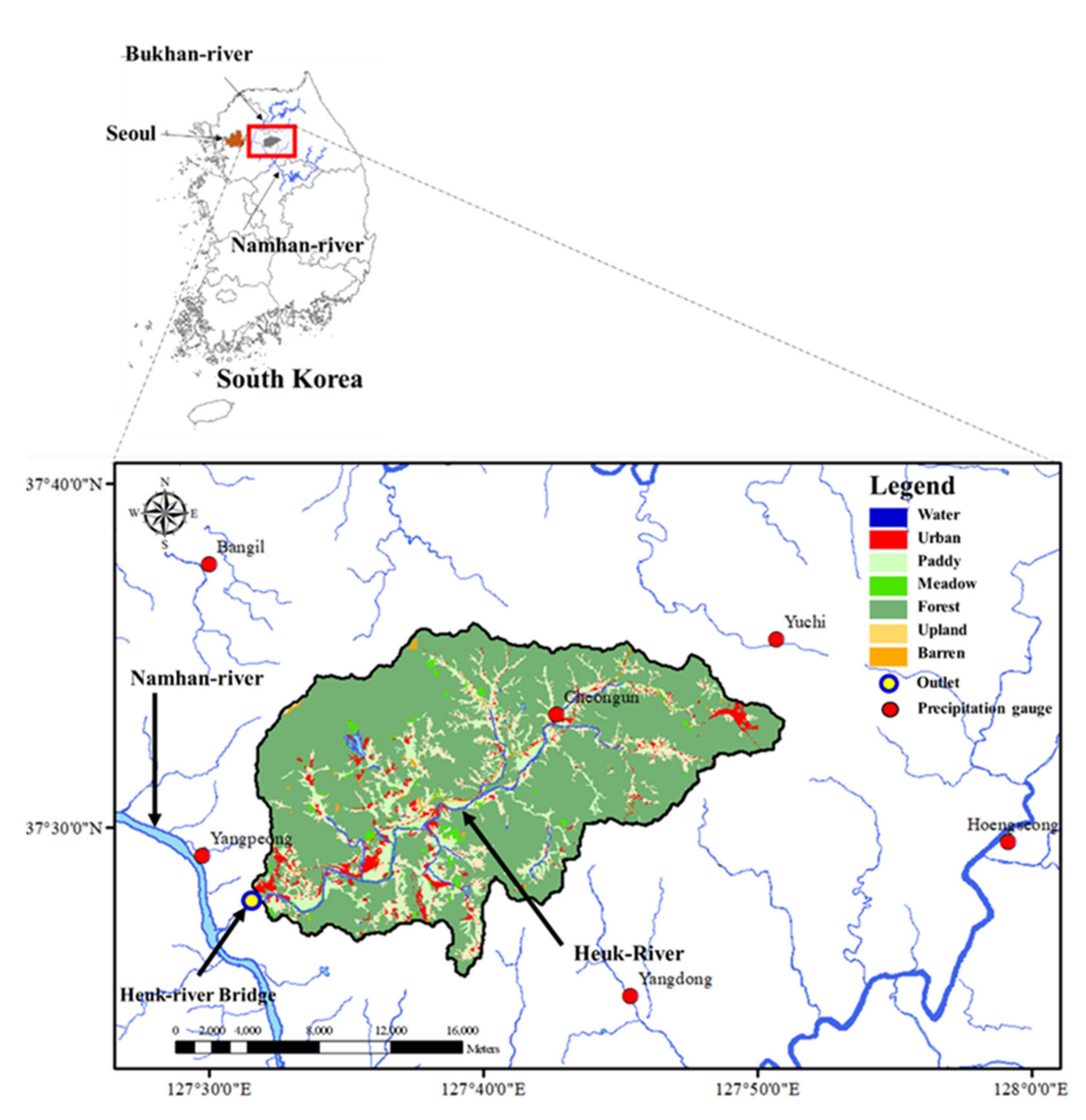
The republic of Korea has been implementing the total maximum daily management (TMDL), which manages the pollutant load of a watershed for the conservation of water quality. To this end, the rep. of Korea had divided the entire country into a watershed unit. Also, this study site is one of the watershed units for TMDL. This study site was Yangpyeong city in the administrative district of Gyeonggi province, South Korea, and the watershed was Heuk River (127°31′55.39′′ E, 37°27′37.69′′ N), which is a sub-watershed of the Han River watershed (Figure 1). In the Heuk River watershed, no rivers flow from other administrative districts and the Heuk River, originating from Seongjibong, Sinron, Cheongun county, Yangpyeong city, is the mainstream. Since it is a highly regulated area (natural conservation area and special measure area for water resource conservation), no significant changes in land use have occurred.
The watershed area of the Heuk River is 314.0 km2. The dominant land-uses are forest (79%) and agricultural region (paddy 8.3%, upland 7.0%). Stream length is 42.9 km, and the average slope is 27°, making it a typical rural area (Table 1).
2.2. Data Collection
Four types of data were required for this study: rainfall, runoff, soil map, and land use data; the data collection period spanned 2006–2019. All data were obtained from online sources; rainfall data were acquired from the Korea Meteorological Administration [18], runoff, and soil maps were acquired from the Water Management Information System [19], and the land use map was obtained from the Environmental Geographic Information Service [20]. The runoff data are daily average data measured at the Heuk River Bridge, as shown in Figure 1, and the rainfall data are daily data from six precipitation gauge sites located inside and outside the study area, as shown in Figure 1. The land use map and soil map are in a grid format with a resolution of 30 m × 30 m and a scale of 1:5000. The land use map comprises seven items (water, urban, paddy, meadow, forest, upland, and barren), and the soil map comprises 59 physical properties of soil.
2.3. Research Method
The CNN model used in this study uses supervised learning as the learning method based on a deep learning algorithm. Accordingly, the CNN model uses input data comprising image data and corresponding target data for learning. The runoff model developed in this study requires input data reflecting meteorological, topographical, and hydrological conditions, which must be image data recognizable by the CNN model, rather than [1 × K] or [K × 1]-dimension numerical data, as used in prior ANN research. Based on these basic conditions for developing this model, the research process applied the following procedures. (1) As mentioned earlier, the image, as an input of the CNN model, should be considered the hydrological phenomena. For this purpose, this study would first like to define the image reflected in the hydrological conditions and propose the methodology of image building. (2) In the second procedure, image data in a two-dimensional [N × M] matrix structure and [1 × K]-dimensional target data were generated and subsequently divided into input and test data sets. The input data set is data for training and testing the model, while the test data set is data for assessing the model’s predictive performance. The input data set was also further divided into a training data set and validation data set. (3) In the third procedure, this study sought to modify the model’s architecture so that the CNN model’s predicted results would simulate continuous values. However, rather than CNN model architectures showing excellent performance in previous research, this study sought to use the most basic CNN model architecture. This was to minimize the influence of the CNN model architecture on the model performance and to allow an evaluation of the CNN model’s applicability for hydrological images built using the curve number. (4) In the fourth procedure, the nonlinear relationship between the feature of the hydrological image in the CNN model and the runoff was learned, after which runoff was predicted. (5) Finally, the recognition of images was reviewed for the CNN model, and the CNN model was evaluated using predicted values, and its suitability and accuracy were analyzed.
2.3.1. Hydrological Image Concept and Construction Method Using Curve Number
The CNN model uses the supervised learning method, which inputs problems (input data) and answers (target data) into a neural network as one data set, and trains the model to find suitable answers for new problems that the model has not previously experienced. Red, green, and blue (RGB) or grayscale images (photograph) were used as input data for the CNN, and an algorithm was used to extract features, such as color values and locations in two-dimensional [N × M] space to solve a problem. In this study, image input data must be recognizable by the CNN. Owing to the nature of this study, there is a difficulty in that numerical images reflecting hydrological phenomenon must be used, rather than general photographic data.
In other words, even if the model using a general RGB photograph as input data has produced a good result regarding predicting runoff, the RGB values in a photograph could collapse the presupposition of the empirical model because they are simply a numerical representation of the color. That is, the runoff has diverse phases caused by various conditions, such as meteorology, land use, and soil characteristics. Herein, if the runoff is estimated with unrelated data, the result value becomes meaningless even if the simulated result’s accuracy is high.
In this study, it was necessary to set up a new concept to distinguish between the image reflecting the hydrological conditions and the RGB photograph, and to this end, this paper proposed the concept of hydrological image. The hydrological image employs the pixel concept of ordinary RGB photography. The hydrologic image follows this mechanism, just as a general photograph presents significant shapes that humans can perceive by the collection of small units of a pixel in two-dimensional space. This paper used the idea of a grid to build the hydrological image, which is usually used to represent a type of map in the Geographic Information System. The grid is applied to a constituent unit of the hydrological image and has a function such as a general photograph’s pixel. Also, the grid has attribute values reflecting the conditions of meteorology, land use, and soil characteristics in a study area. Thus, the hydrological image could be defined as a set of grids with a hydrological attribute value in a two-dimensional space for a discretionary watershed.
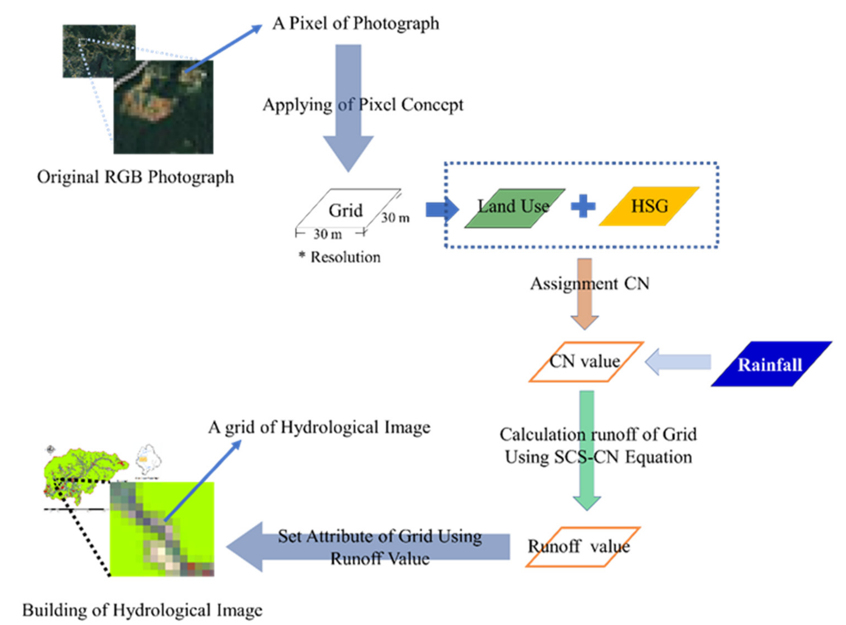
The hydrological image employs the curve number (CN) method published by the Soil Conservation Service (SCS), the predecessor of the National Resource Conservation Service (NRCS), to calculate the attribute of the grid, as shown in Figure 2. To implement the phenomena of runoff regarding rainfall, soil characteristics, and land use, the CN is an effective method used globally for evaluating the hydrological influence [21,22]; as such, building a hydrological image using CN was deemed suitable for this study.
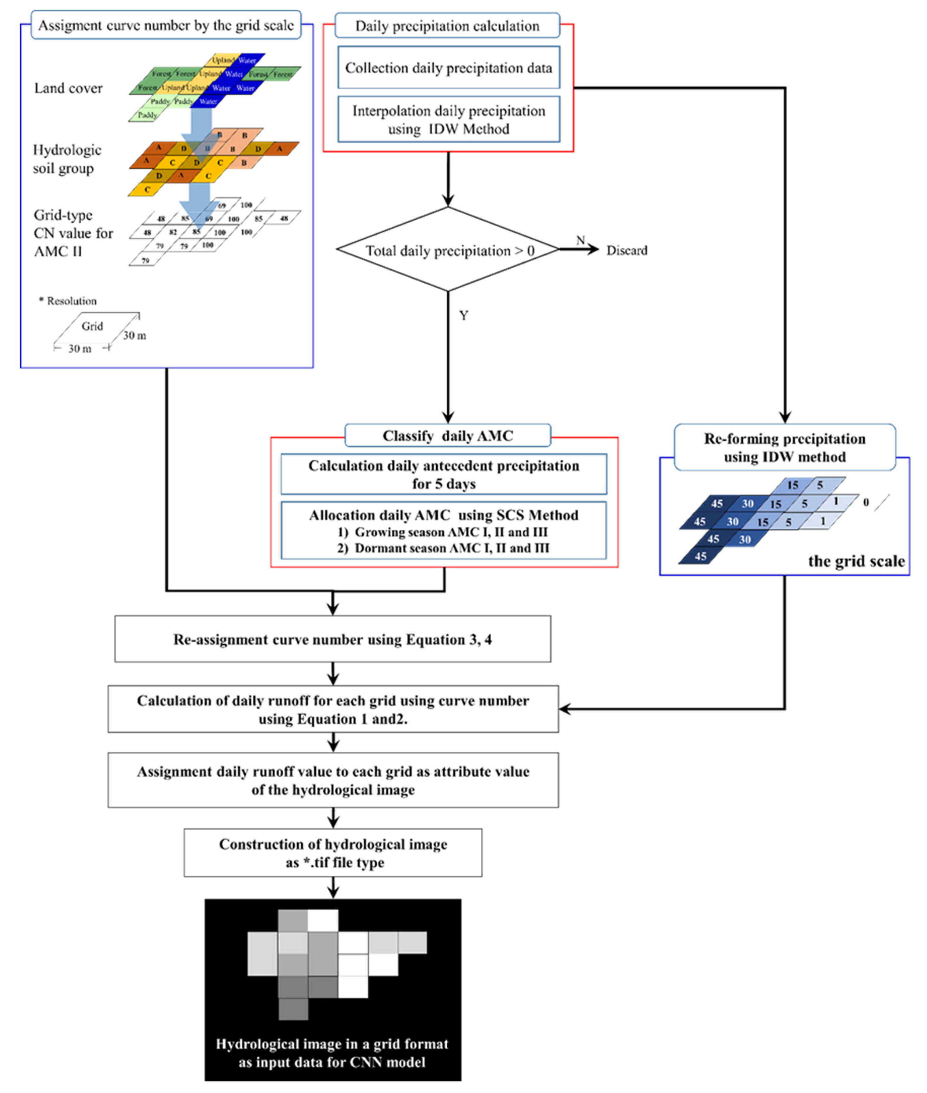
The CN method is a standardized approach for flood risk assessment and flood-related research [23,24,25]. Runoff could be calculated by directly reflecting influences, including the soil physical properties, land use, land management, and antecedent soil moisture conditions (AMC) [26,27], and runoff could be estimated according to the CN value. The CN method, basically, proposes to assign CN values using land use and soil physical properties. The CN method divides the physical properties of soil into four physical properties, such as hydrology soil group (HSG), and uses these values to allocate CN. Therefore, in this study, the collected soil map was classified into HSG according to the CN method and utilized for CN values allocation.
In the preceding study, generally, the representative CN [28,29,30] of the whole study site, or the area-weighted mean CN assignment method [31,32] had been applied to simulate the direct runoff. However, these methods were unsuitable for this study. Using a representative CN or area weighted CN resulted in very monotonous images, and it became very difficult to extract image features from such images. Accordingly, this study generated hydrological images by assigning the CN to each grid in the hydrological image, just by giving a value to pixels, the basic unit comprising photos, thereby obtaining an effect similar to the characteristics of a general photo. The unit for the CN assignment was set to the same grid and spatial resolution (30 m × 30 m) of the land use and HSG. The CN assignment method using land use and HSG had been proposed by the SCS, so this study assigned the CN in each grid through the same CN method. In the next process, this study estimated the runoff in each grid. The value calculated by the CN in the grid is the runoff value with the unit m3/s, but in this study, it was set to a non-dimensional numerical value and assumed to be the attribute value of each grid to use on the hydrological image.
If images are created by assigning the CN without considering the hydrological conditions, then there are no changes because the CN is a constant, and it cannot act as a variable since all generated hydrological images take the same value.
Rainfall data are necessary to calculate the amount of runoff for each grid. As the rainfall required to calculate runoff must be matched to the grid units, this study used the inverse distance weighted (IDW) method to calculate the rainfall rather than the Thiessen polygon method, which is traditionally used for this purpose. Using Thiessen polygons causes discontinuities in the numerical changes at polygon boundaries, leading to distortions or differences compared with the actual rainfall. In contrast, IDW, an interpolation method based on Tobler’s law, can be used to compensate for the discontinuities of Thiessen polygons and calculate rainfall data in a grid format with 30 m × 30 m resolution, consistent with the land use and HSG. As shown in Figure 1, this study used rainfall data from six rainfall monitoring stations as the input data of the IDW tool of ArcGIS 10.0 to generate rainfall data in a grid format with 30 m × 30 m resolution.
To calculate the runoff for each grid, this study used Equations (1)–(3), with the initial abstraction set to 0.2, as proposed in the SCS.
where Q is runoff, P is rainfall, and S is potential retention storage. Though the CN value is provided by SCS, it is not suitable for use in Korea because the topographical conditions are different from the United States. Therefore, this study used the CN provided in the Guideline of Design Flood Estimation of the Ministry of Land, Transport and Maritime Affairs of ref. of Korea [33].
As the CN in Equation (2) corresponds to AMCII, it does not consider the AMC, and when calculating runoff using CN under a consistent AMCII, a large error occurs between the actual and predicted value. Accordingly, SCS proposes calibrating the CN according to conditions such as 5-day accumulated rainfall and change in AMC for dormant and growing seasons. Consequently, this study calculated the 5-day accumulated rainfall for each day, classified this as dormant and growing seasons, derived AMCI, AMCII, and AMCIII, and recalculated CN as CNI and CNIII using Equations (4) and (5) as a function of AMC.
where CNI is the value for AMCI, and CNIII is the value for AMCIII.
As the final step, and because of the above-mentioned reasons, as the image of the dry period is a fixed CN value, these data were discarded, and only data corresponding to periods of rainfall were collected. These data were converted to TIF image files, while maintaining the same two-dimensional structure as the land use and HSG, and used the CNN model input data for building the model. When using JPG, BMP, or PNG file formats, runoff information, a grid property value, is converted to a new value when the data are converted to a color value, ranging from 0–255, resulting in information loss. For this reason, the TIF format was used instead.
As shown above, the hydrological image describes literally hydrological phenomena and is a suitable means to express the watershed condition. However, this study’s hydrological image has a limitation because it does not include all hydrological processes. Nevertheless, it would be adequate to adopt a methodology for building input data of the CNN model.
2.3.2. Target Data
Target data was constructed by daily average runoff data, and the date of target data must correspond to the data of the hydrological image. As mentioned above, data for the CNN model training must constitute input and target data in one data set. Unlike complex image generation methods, runoff data corresponding to the date of the generated image were simply used as the target data, which were constructed as a CSV type file.
2.3.3. CNN Model Architecture Configuration
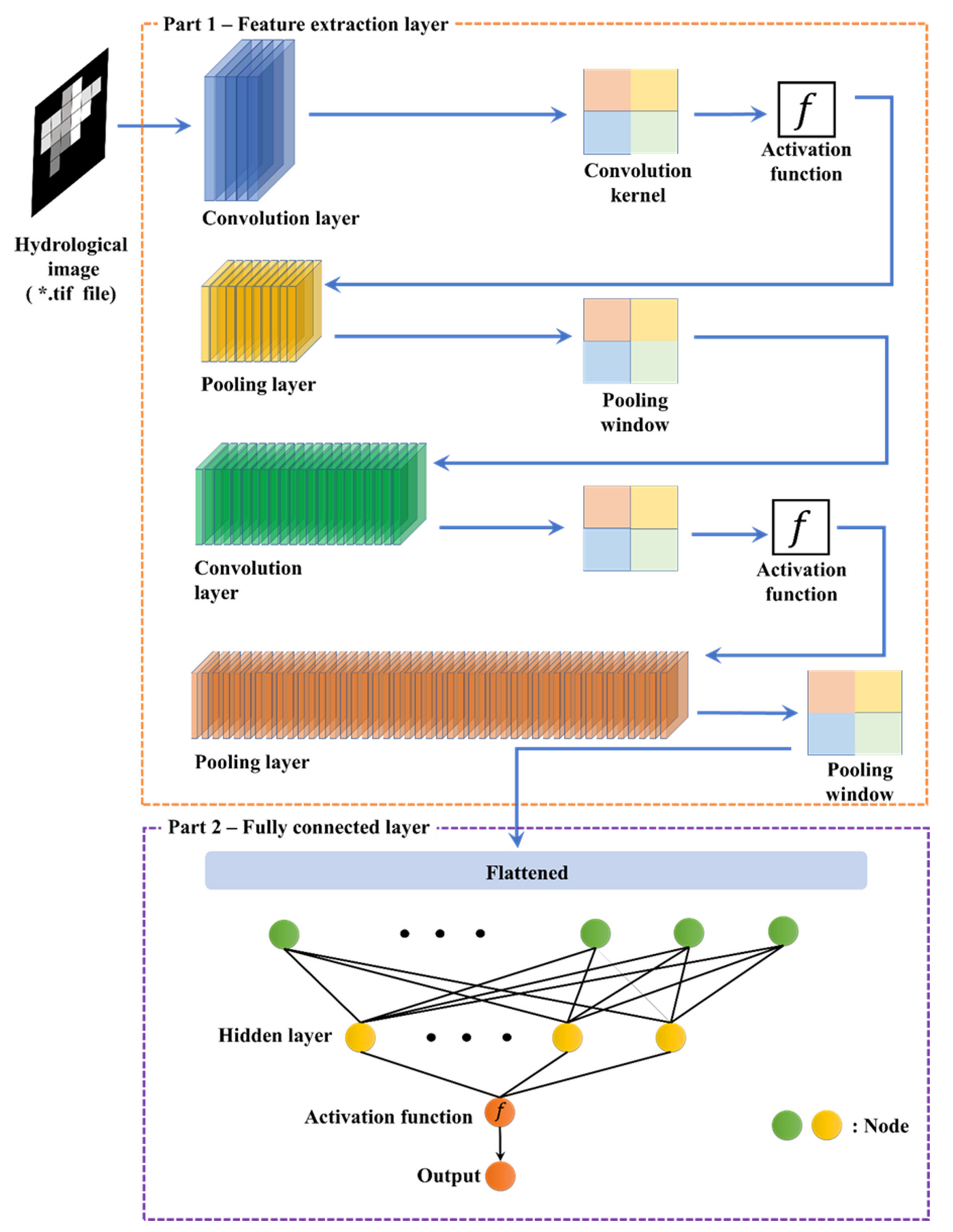
CNN, a deep learning architecture, is a model inspired by the way the brain’s visual cortex works when recognizing objects. A CNN model consists of an input layer, hidden layers, and an output layer, similar to existing ANNs. However, as shown in Figure 4, two parts constitute the neural network specialized for recognition and classification of an observed image. Part 1 of Figure 4 is a layer that extracts image features, a core function of the CNN model, and comprises repeated convolution and pooling layers. Part 2 of Figure 4, a fully connected layer that recognizes the image features output from Part 1 of Figure 4 as the input layer, is a deep neural network comprising numerous hidden layers between the output layers [35,36].
The use of the CNN model architecture in this study has two main objectives, the first was to maintain the image features extraction function by repeating the convolution and pooling layers, as shown in Part 1 of Figure 4, and the second was to change the architecture of the fully connected layer in Part 2 of Figure 4 to enable simulation of unspecified continuous variables.
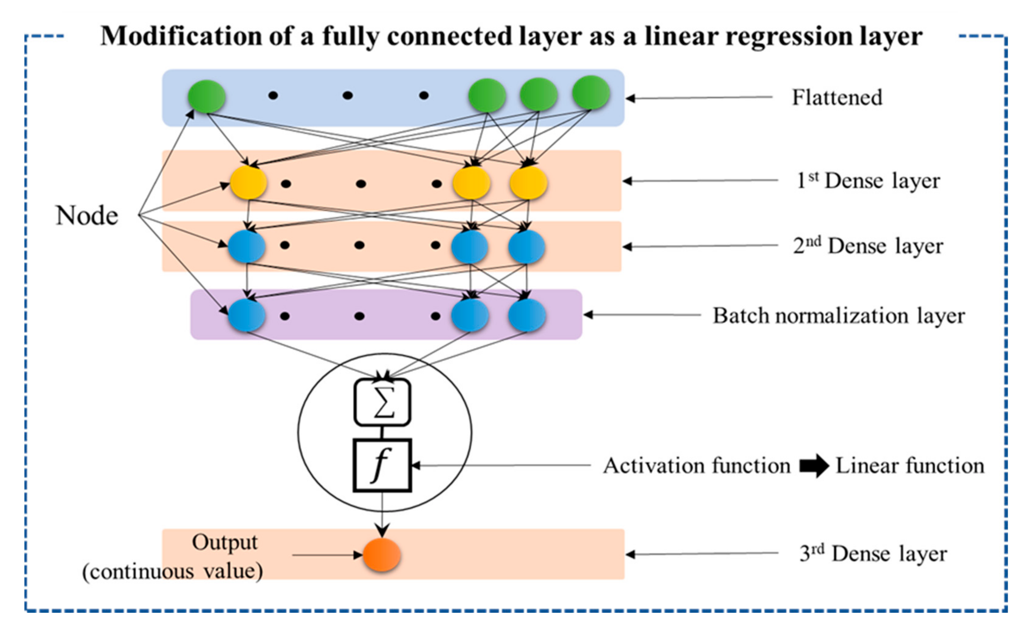
For this purpose, the architecture of Part 1 of Figure 4 is the most general; the convolution and max-pooling layers intersect to form a structure with five repetitions. In general, Part 2 of Figure 4 receives the two-dimensional image features extracted from Part 1 of Figure 4, converts them to one dimension through the flatten function, and uses them as the input values of the fully connected layer. In particular, in Part 2 of Figure 4, in line with the CNN model’s objectives, the softmax, the binary cross-entropy, or the categorical cross-entropy function were used as the activation function of the last layer of the fully connected layer to solve the classification problem. However, as the runoff value to be simulated in this study is an unspecified continuous variable, the last layer of the fully connected layer architecture is unsuitable without some modification. Therefore, part 2 of Figure 4 must be modified. For modification to a linear regression layer suitable for deriving unspecified continuous variables, as shown in Figure 5, the activation function of the last layer was set as a linear function, and a dense layer of three layers and a batch normalization layer were added to avoid overfitting. The environment for the CNN model design, implementation, and operation was Keras, with Tensorflow as the backend [37], a machine learning library published by Google. The implementation and experimentation were conducted through Python. Keras, a high-level DNN application programming interface (API) written in Python, supports all the special functions of Tensorflow and has high DNN model implementation flexibility. Moreover, it enables quick experimentation by efficiently using the CPU and GPU [38].
The CNN model was trained on Window-OS PC that has the Intel® Core ™ i9-9900K CPU @ 3.60GHz, 32G RAM, and NDIVIA® GEFORCE RTX ™ 2080Ti GPU.
2.3.4. Detailed CNN Model Settings
The convolution layer operation uses a separate two-dimensional plane function called a kernel, a type of image filter, and kernel size can be arbitrarily set in Keras. In this model, the kernel of the first convolution layer was set to a size of 5 × 5, and those of the remaining convolution layers were set to a size of 2 × 2. The number of kernels was also specified as to 32, 64, 128, 256, and 512 in the five convolution layers in the respective order of layers. The activation function of all convolution layers was also set to a rectified linear unit function (ReLu), which is typically used in CNN models. Through this, gradient vanishing can be avoided, and high optimization efficiency of the model can be achieved [39,40].
The pooling layer, a sub-sampling technique that reduces the image size and leaves only important information of the image, enables the efficient use of computer memory and prevents overfitting by reducing the calculated information. Pooling methods include max and average-pooling, as average pooling can result in information loss of the image, max-pooling was employed in this model. Pooling size can also be specified and was set to 2 × 2 in this study. Hence, the size was halved each time the image goes through the layer.
Table 2 shows the CNN model architecture of this study. In Table 2, there are 5,272,321 total parameters, which represent the number of neural network weights, comprising 5,272,065 trainable parameters and 256 non-trainable parameters. Finally, the activation function of the last dense layer was set as a linear function to allow continuous variables to be derived, and the number of nodes was set to 1 to match the target data.
For model training, the loss function was set and optimized by updating the parameter values of the iterative neural network, using an optimizer algorithm. Thus, it is important to reduce the error between the actual value and the predicted value. In the field of neural networks, stochastic gradient descent (SGD) [41] is considered the most basic optimizer algorithm methodology. Each time a parameter was updated, SGD obtains the gradient through differentiation and then reduces loss, while updating towards a lower gradient. Loss is similar in concept to error, and DNNs typically train to reduce loss. Here, “stochastic” means to stochastically obtain some samples and divide them gradually rather than calculate all the parameters simultaneously. If the epochs are sufficient, then SGD is effective, though it has the disadvantage of severe noise and slow speed. The optimization algorithms have recently been used, including Momentum [42], Nesterov Accelerated Gradient (NAG) [43], Adagrad [44], Nadam [45], Adadelta [46], RMSProp [47], and Adam [48], and these enhance training speed and accuracy. RMSProp exhibits better training results than both Adagrad and Adadelta, the latter of which improves on Adagrad’s weaknesses. Moreover, as RMSProp can apply Momentum, the translation vector for the previous gradient could be applied by applying the Momentum constant. Therefore, it has been extensively used with Adam. Therefore, RMSProp was employed as the optimizer function of CNN in this study.
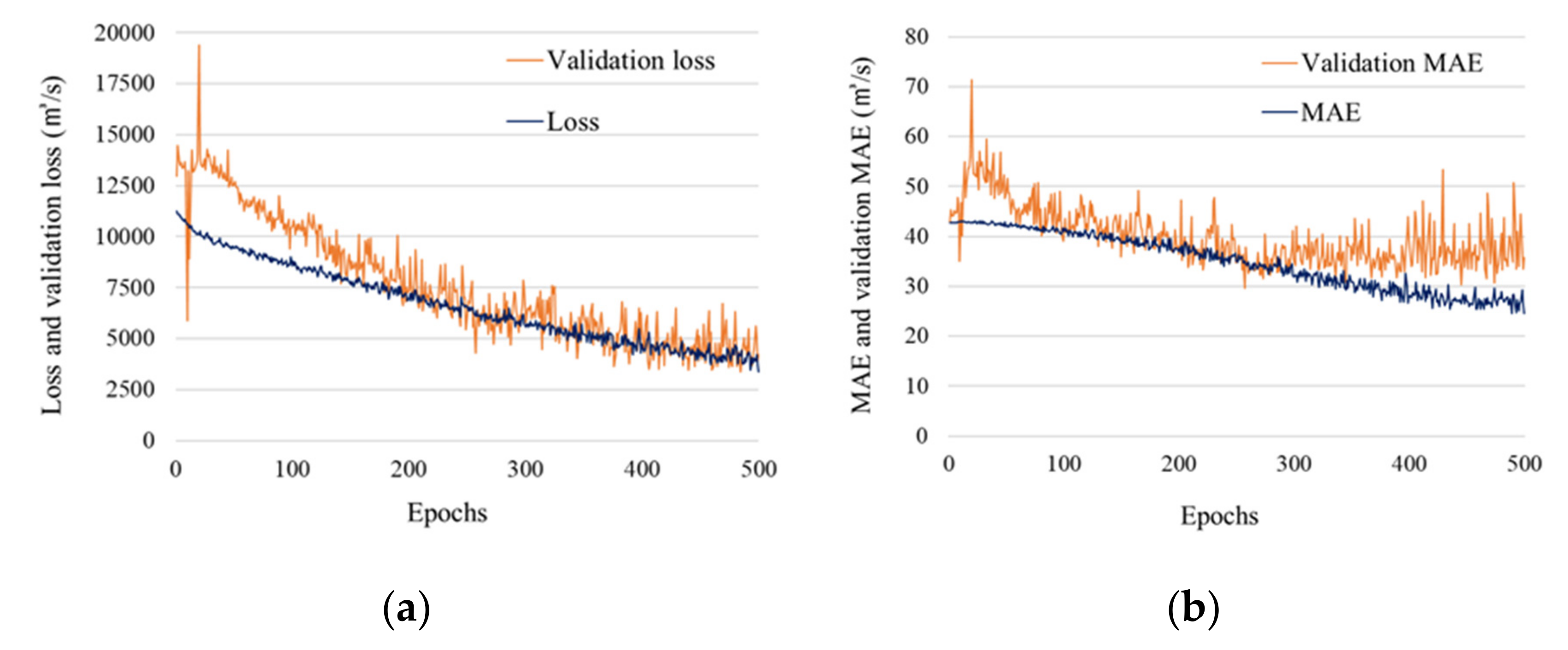
In addition, accuracy is commonly used as a metric to generalize CNN models and evaluate their training results, and mean absolute error (MAE) is used as a metric for continuous variable prediction. Accordingly, in this study, the loss function was set to mean square error (MSE), as in Equation (6), the parameter optimization algorithm was set to RMSProp, the learning rate was 1.0 × 10⁻⁴, and the epoch was set to 500. Mean absolute error (MAE) was also used as a metric of the model, as described in Equation (7).
where and indicate the actual and predicted values, respectively. In addition, the more MSE and MAE converge to 0, the higher the model’s performance. The model’s training results are evaluated using the results of loss, validation loss, MAE, and validation MAE. Among the input data sets, loss and MAE are for the training data set and indicate the model’s training results and prediction performance, respectively, while validation loss and validation MAE are for the validation data set and indicate the model’s training results and prediction performance for generalization.
2.3.5. Model Evaluation Criteria
The model was evaluated by judging its performance through comparisons of the actual value and the value predicted through the model. Three methods were used for this purpose: Pearson correlation coefficient (), Nash–Sutcliffe efficiency (NSE), and root mean square error (RMSE).
Pearson correlation coefficient is expressed in the range of −1 to 1 through Equation (8) and indicates the linearity between the actual value and predicted value. The closer is to 1, the stronger the linearity between the actual and predicted values, and the more it converges to 1, the better the model’s performance.
The Nash–Sutcliffe efficiency is expressed in Equation (9); a result of 1 signifies that the model’s result and actual value are perfectly matched. In addition, the more it converges to 0, the lower the model’s performance.
Root mean square error expresses how close the model’s prediction is to the actual value through Equation (10), which ranges from 0 to infinity within the scope of the corresponding data. Though the evaluation standard for RMSE itself is unclear, the more it approaches 0, the more consistent the model’s result with the actual value.
where and are the actual value and predicted value, respectively, and and are averages of the actual value and predicted value, respectively.
3. Results and Discussion
3.1. Building Results of the Hydrological Image Data and Target Data
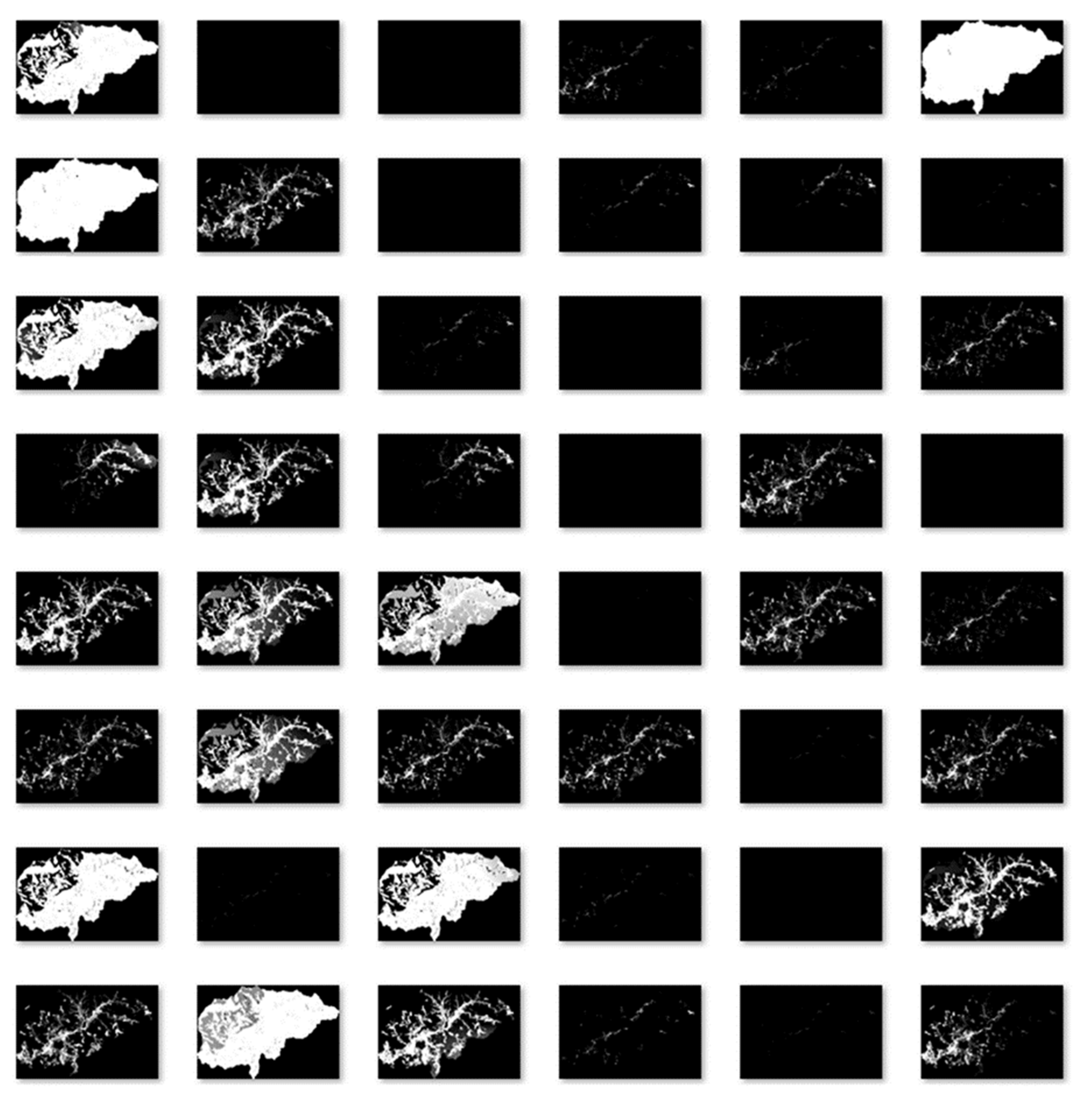
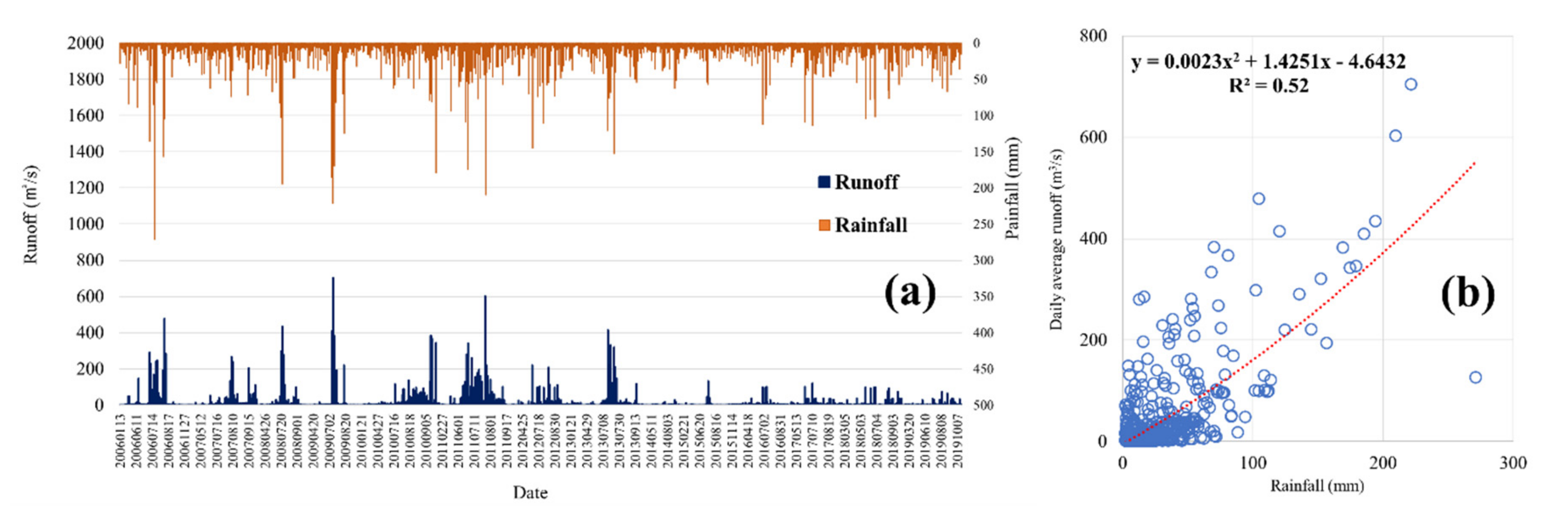
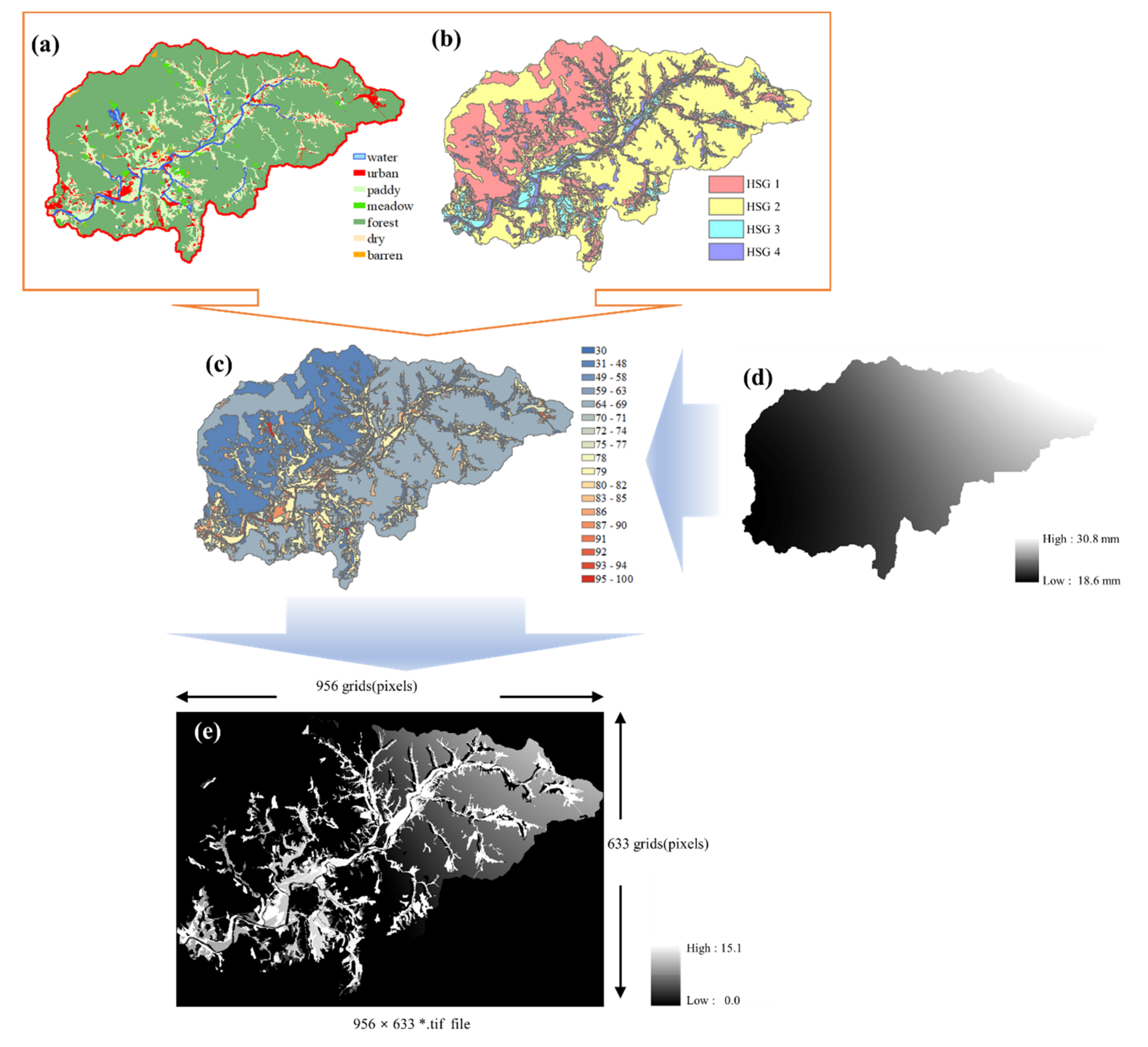
During the data collection period, there were 680 occurrences of events exceeding the effective daily rainfall, resulting in 680 hydrological images. Figure 6 shows only part of the building results of 680 hydrological images due to the limitations of the space of paper. Figure 7 denotes the target data corresponding to the hydrological image, which means the runoff with a range of 0.18–704.27 m3/s, and this runoff data as the target data were converted into the CSV file for applying to the CNN model. The actual processing of the hydrological image is presented in Figure 8, as mentioned in Section 2.3.1. Figure 8a shows the land use status in a grid before image generation, b shows HSG, c shows CN by a–d shows the rainfall distribution by IDW, and e shows the image, i.e., the finally generated hydrological image as the CNN input data. This image comprises 956 and 633 grids on the horizontal and vertical axes and is saved as a TIF file. In Figure 8d, areas closer to white indicate higher rainfall, and areas closer to black indicate lower rainfall. In the grayscale image of Figure 8e, as in Figure 8d, areas closer to white indicate higher runoff and areas closer to black indicate runoff converging to 0. While Figure 8e follows the rainfall distribution shown in Figure 8d, the brightness is judged to differ with the CN value.
The 680 final hydrological images and corresponding 680 target data (runoff data) were input into the CNN model together as one data set. However, to divide these into the input data set and test data set, 501 data points (approximately 70%) were used as the input data set for training the CNN model, and the remaining 179 data points were used as the test data set to evaluate the model’s predictive performance. Furthermore, 400 data points (80%) of the input data set were classified as the training data set, and the remaining 101 were used as the validation data set to validate the model. The criterion for data classification is unclear and mostly arbitrarily set by researchers; many previous studies have used 7:3 or 8:2 ratios of input: test data for experimentation [49,50,51,52,53,54].
3.2. Model Training Results
The CNN model run at around 1.3 s per epoch, and the total time spent on CNN model training was shown to be about 650 s. Figure 9 shows the model training results. s. Figure 9a shows loss and validation loss, and Figure 9b shows MAE and validation MAE. When the model was stably trained the change in loss, validation loss, MAE, and validation MAE were similar to an exponential function with base 0, or less. Loss began from 11,264.26 m3/s in the first epoch and steadily decreased to 3372.72 m3/s in the last epoch (Figure 9a). The validation loss initially exhibited unstable changes; however, it gradually decreased as the epochs progressed, from 12,980.25 m3/s in the first epoch to 4199.01 m3/s in the last epoch, indicating that model training and generalization were stably performed. Mean absolute error, which expresses the change in error between the actual and predicted values of the model, began at 42.68 m3/s in the first epoch and steadily decreased to 24.58 m3/s in the last epoch (Figure 9b). This signifies that as the model training progressed, the model’s simulated predictions gradually approached the actual values. In contrast, while the validation MAE exhibited unstable changes in the early epochs similar to the validation loss, it gradually decreased as the epochs progressed. After passing the 250th epoch, however, it exhibited unstable changes, though it ultimately showed a decreasing trend, indicating that the model generalization for the validation step was also apparent.
3.3. Prediction Results and Model Evaluation
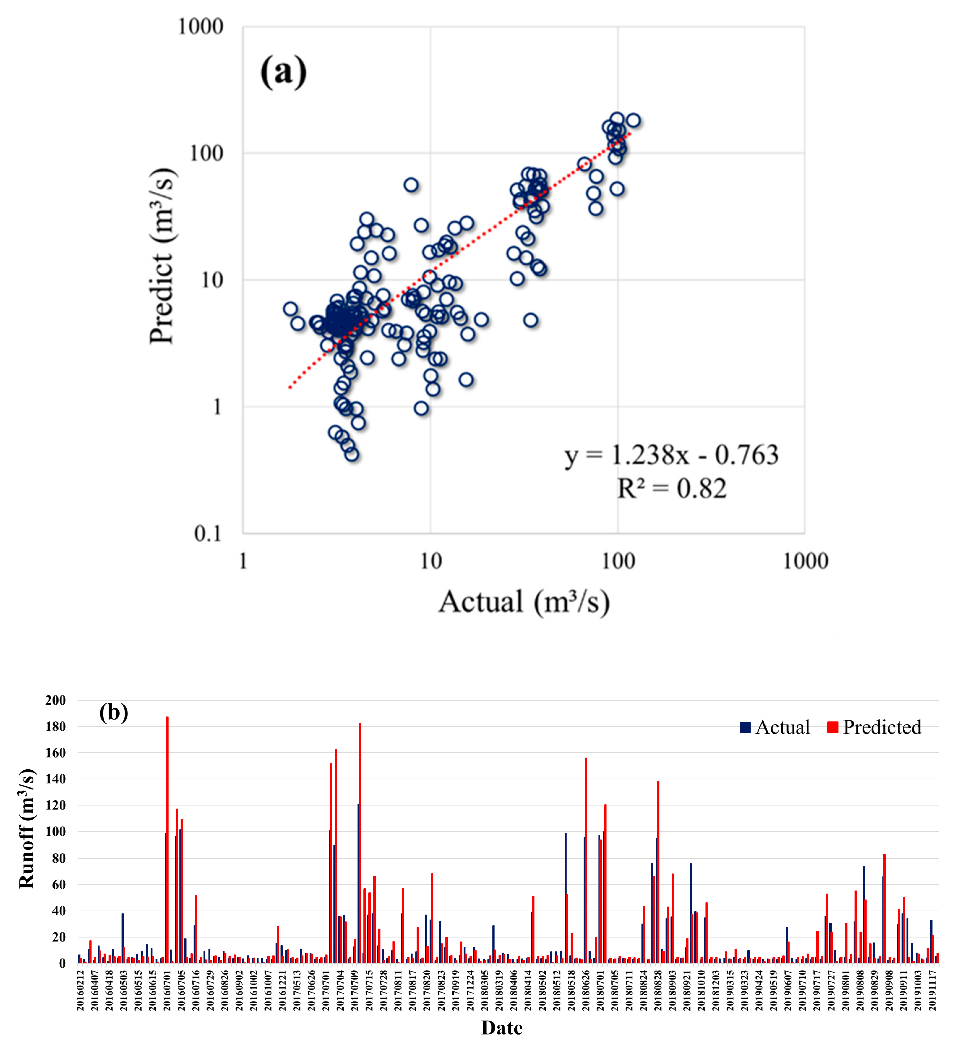
The test data set described above was used to evaluate the model’s performance. Figure 10 shows the dispersion of the model’s predicted and actual values. R2, which indicates the relationship between the actual and predicted value, was relatively high at 0.83 in Figure 10a. Figure 10b shows the change of the predicted and actual values; the x-axis represents the date of the 179 images in the test data set, and the y-axis represents the predicted value and actual value based on the image. The predicted values showed a similar trend to the actual values overall.
Table 3 shows the r, NSE, and RMSE to evaluate the model. The r value was 0.87, indicating a very high correlation between the predicted and actual values. For NSE, values of 0.60–0.80 are generally judged as moderate to good, and values exceeding 0.80 as good [55]. As NSE in this model was 0.60, its performance could be judged as moderate. RMSE was 16.20 m3/s, which was similar to the MAE (24.58 m3/s), the final training result of the model. Accordingly, the evaluation of the CNN model modified to enable the simulation of watershed images was generated considering the CN, rainfall, and AMC as continuous variables, demonstrated good training results and good overall predictive performance.
Although there have been few studies employing similar approaches to that presented herein, Sundara Kumar et al. [56] used an ANN similar to the ANN corresponding to Part 2 of the model developed in this study and developed a rainfall-runoff model using an ANN consisting of only an input layer, hidden layers, and an output layer, and evaluated their model. Their MAE ranged from 5.04 mm to 9.99 mm and the RMSE ranged from 8.24 mm to 16.83 mm, across five watersheds, indicating that their model appropriately reflected the actual values. Kashani et al. [57] divided the research watershed into sub-watersheds, developed an ANN for each sub-watershed, and simulated the rainfall-runoff for the entire watershed. The r value was 0.94, RMSE was 2.14 m3/s, and NSE was 0.68 m3/s, indicating slightly higher model performance than the present study. Kasiviswanathan et al. [58] developed three lead-time and five lead-time rainfall-runoff predictive models through ANN based on ensemble simulations using a genetic algorithm. RMSE of the calibration data of the three lead-time ANN was 66.35–73.20 m3/s, and NSE was 84.29–87.33%, while RMSE of the validation data was 59.12–65.72 m3/s, and NSE was 87.95–70.24%. Similarly, RMSE of the calibration data of the five lead-time ANN was 31.55–111.49 m3/s, and NSE was 64.22–75.06%, while RMSE of the validation data was 89.16–119.41 m3/s and NSE was 60.44–77.94%, demonstrating that the three lead-time ANN had better performance. Guo et al. [59] developed an ANN and incomplete-connection ANN and compared the two; RMSE of the ANN was 47.27 m3/s, and R2 was 0.55, while RMSE of the incomplete-connection ANN was 24.55 m3/s and R2 was 0.88, demonstrating improved model performance. Maca et al. [60] developed rainfall-runoff models using 12 functions as the ANN activation functions, including logistic sigmoid, hyperbolic tangent, linear function, Gaussian function, and root sigmoid and compared their performances. The NSE of the root sigmoid function was the highest at 0.70, indicating that the root sigmoid function was appropriate as an activation function. Machado et al. [61] developed a monthly rainfall-runoff prediction model using an ANN. According to 60-month simulation results, R2 was 0.71, and NSE was 0.71; for 120 months, R2 was 0.92 and NSE was 0.92; and for 180 months, R2 was 0.94 and NSE was 0.88. Hence, the 120-month simulation demonstrated the best results. Accordingly, this study’s model showed a similar performance to those of previous studies, which is attributed to the following: the training function of the linear regression layer designed in this study progressed smoothly, and as the feature values of the images extracted in Part 1 were smoothly injected into training, the hydrological images built using the CN also had enough hydrological information to simulate runoff, enabling them to serve as input data for the CNN model.
4. Conclusions
This study sought to develop a runoff model using a CNN, which is a type of DNN algorithm. Through this methodology, the feasibility of applying a DNN to improve information processing and information throughput was assessed, with the aim of promoting change in the runoff model development methodologies. For this purpose, a methodology was proposed that maintains the ability to extract images while utilizing the convolution and pooling layers, the core functions of the CNN model, and modified the fully connected layer into a linear regression layer to enable the CNN model to simulate unspecified continuous variables. In this regard, the CNN model had previously only been used for classification problems. In addition, a method for generating hydrological images using the CN to build the input data of the CNN model was proposed. The training results of the model developed in this study demonstrated good predictive performance, and the hydrological images built using the CN showed sufficient functionality as the CNN’s input data. Furthermore, this study used the CN, which was traditionally used for estimating runoff, as a tool for generating hydrological images, the CNN model input data. As such, this study presented a new usage of the CN.
This study used the most basic CNN model architecture to minimize the influence of the CNN model architecture on the model performance and to evaluate the CNN’s applicability for hydrological images built using the CN. However, a limitation of this study was the need to enhance accuracy by applying an improved CNN model architecture. Nevertheless, as there are almost no prior studies on runoff simulation using the CNN model comparable to this study, this study is considered to be a preliminary study of runoff simulation techniques using hydrological images. Therefore, the methodology proposed in this study could be gradually developed for use in runoff simulation research applying remote sensing technology or to enable global or regional real-time runoff simulations using satellite images. As such, the utilization scope of the technology is judged to be very large.
Funding
This research received no external funding.
Conflicts of Interest
The author declares no conflict of interest.
References
- Kimura, N.; Yoshinaga, I.; Sekijima, K.; Azechi, I.; Baba, D. Convolutional Neural Network Coupled with a Transfer-Learning Approach for Time-Series Flood Predictions. Water 2020, 12, 96. [Google Scholar] [CrossRef] [Green Version]
- Othman, F.; Naseri, M. Reservoir inflow forecasting using artificial neural network. Int. J. Phys. Sci. 2011, 6, 434–440. [Google Scholar] [CrossRef]
- Maier, H.; Jain, A.; Dandy, G.; Sudheer, K.P. Methods used for the development of neural networks for the prediction of water resource variables in river systems: Current status and future directions. Environ. Model. Softw. 2010, 25, 891–909. [Google Scholar] [CrossRef]
- Nourani, V.; Komasi, M.; Alami, M.T. Hybrid Wavelet—Genetic Programming Approach to Optimize ANN Modeling of Rainfall—Runoff Process. J. Hydrol. Eng. ASCE 2017, 17, 724–741. [Google Scholar] [CrossRef]
- Tokar, A.S.; Markus, M. Precipitation-runoff modeling using artificial neural networks and conceptual moldes. J. Hydrol. Eng. 2000, 5, 156–161. [Google Scholar] [CrossRef]
- Patel, B.; Joshi, G.S. Civil Modeling of Rainfall-Runoff Correlations Using Artificial Neural Network—A Case Study of Dharoi Watershed of a Sabarmati River Basin. CEJ 2017, 3, 78–87. [Google Scholar] [CrossRef]
- Salas, F.R.; Somos-Valenzuela, M.A.; Dugger, A.; Maidment, D.R.; Gochis, D.J.; David, C.H.; Yu, W.; Ding, D.; Clark, E.P.; Noman, N. Towards real-time continental scale streamflow simulation in continuous and discrete space. J. Am. Water Resour. Assoc. 2018, 54, 7–27. [Google Scholar] [CrossRef]
- Akhtar, M.K.; Corzo, G.A.; van Andel, S.J.; Jonoski, A. River flow forecasting with artificial neural networks using satellite observed precipitation pre-processed with flow length and travel time information: Case study of the Ganges river basin. Hydrol. Earth Syst. Sci. 2009, 13, 1607–1618. [Google Scholar] [CrossRef] [Green Version]
- Kalteh, A.M. Rainfall-runoff modelling using artificial neural networks (ANNs): Modelling and understanding. CJES 2008, 6, 53–58. [Google Scholar] [CrossRef]
- Mishra, P.K.; Karmakar, S. Performance of optimum neural network in rainfall-runoff modeling over a river basin. IJEST 2019, 16, 1289–1302. [Google Scholar] [CrossRef]
- Shoaib, M.; Shamseldin, A.Y.; Melville, B.W.; Khan, M.M. A comparison between wavelet based static and dynamic neural network approaches for runoff prediction. J. Hydrol. 2016, 535, 211–225. [Google Scholar] [CrossRef]
- Farias, C.A.; Santos, C.A.; Lourenço, A.M.; Carneiro, T.C. Kohonen neural networks for rainfall-runoff modeling: Case study of piancó river basin. JUEE 2013, 7, 176–182. [Google Scholar] [CrossRef] [Green Version]
- Zhang, B.; Govindaraju, R.S. Prediction of watershed runoff using Bayesian concepts and modular neural networks. Water Resour. Res. 2000, 36, 753–762. [Google Scholar] [CrossRef]
- Wilby, R.L.; Abrahart, R.J.; Dawson, C.W. Detection of conceptual model rainfall—Runoff processes inside an artificial neural network. Hydrol. Sci. J. 2003, 48, 163–181. [Google Scholar] [CrossRef] [Green Version]
- Jain, A.; Sudheer, K.P.; Srinivasulu, S. Identification of physical processes inherent in artificial neural network rainfall runoff models. Hydrol. Process. 2004, 18, 571–581. [Google Scholar] [CrossRef]
- Sudheer, K.P.; Jain, A. Explaining the internal behaviour of artificial neural network river flow models. Hydrol. Process. 2004, 18, 833–844. [Google Scholar] [CrossRef]
- Taravat, A.; Del Frate, F.; Cornaro, C.; Vergari, S. Neural networks and support vector machine algorithms for automatic cloud classification of whole-sky ground-based images. IEEE Trans. Geosci. Remote Sens. 2015, 12, 666–670. [Google Scholar] [CrossRef]
- KMA: Korea Meteorological Administration. Available online: https://www.kma.go.kr (accessed on 3 January 2020).
- WAMIS: Water Management Information System, National Institute of Environmental Research. Available online: https://www.water.nier.go.kr (accessed on 1 March 2019).
- EGIS: Environmental Geographic Information Service. Available online: https://www.egis.me.go.kr (accessed on 9 January 2019).
- Li, C.; Liu, M.; Hu, Y.; Shi, T.; Zong, M.; Walter, M.T. Assessing the impact of urbanization on direct runoff using improved composite CN method in a large urban area. Int. J. Environ. Res. Public Health 2018, 15, 775. [Google Scholar] [CrossRef] [Green Version]
- Wang, H.; Chen, Y. Identifying key hydrological processes in highly urbanized watersheds for flood forecasting with a distributed hydrological model. Water 2019, 11, 1641. [Google Scholar] [CrossRef] [Green Version]
- Li, F.; Chen, J.; Liu, Y.; Xu, P.; Sun, H.; Engel, B.A.; Wang, S. Assessment of the impacts of land use/cover change and rainfall change on surface runoff in China. Sustainability 2019, 11, 3535. [Google Scholar] [CrossRef] [Green Version]
- Yang, L.; Feng, Q.; Yin, Z.; Wen, X.; Si, J.; Li, C.; Deo, R. Identifying separate impacts of climate and land use/cover change on hydrological processes in upper stream of Heihe River, Northwest China. Hydrol. Process. 2017, 31, 1100–1112. [Google Scholar] [CrossRef]
- Soulis, K.X. Estimation of SCS Curve Number variation following forest fires. Hydrol. Sci. J. 2018, 63, 1332–1346. [Google Scholar] [CrossRef]
- Ling, L.; Yusop, Z.; Yap, W.-S.; Tan, W.L.; Chow, M.F.; Ling, J.L. A calibrated, watershed-specific SCS-CN method: Application to Wangjiaqiao Watershed in the Three Gorges Area, China. Water 2020, 12, 60. [Google Scholar] [CrossRef] [Green Version]
- Krajewski, A.; Sikorska-Senoner, A.E.; Hejduk, A.; Hejduk, L. Variability of the Initial Abstraction Ratio in an urban and an agroforested catchment. Water 2020, 12, 415. [Google Scholar] [CrossRef] [Green Version]
- Ajmal, M.; Waseem, M.; Kim, D.; Kim, T.-W. A Pragmatic Slope-Adjusted Curve Number Model to Reduce Uncertainty in Predicting Flood Runoff from Steep Watersheds. Water 2020, 12, 1469. [Google Scholar] [CrossRef]
- Zhang, D.; Lin, Q.; Chen, X.; Chai, T. Improved Curve Number Estimation in SWAT by Reflecting the Effect of Rainfall Intensity on Runoff Generation. Water 2019, 11, 163. [Google Scholar] [CrossRef] [Green Version]
- Deshmukh, D.S.; Chaube, U.C.; Ekube, A.H.; Aberra, D.G.; Tegene, M.K. Estimation and comparison of curve number based on dynamic land use land cover change, observed rainfall-runoff data and land slope. J. Hydrol. 2013, 492, 89–101. [Google Scholar] [CrossRef]
- Pal, S.C.; Chakrabortty, R. Simulating the impact of climate change on soil erosion in sub-tropical monsoon dominated watershed based on RUSLE, SCS runoff and MIROC5 climatic model. Adv. Space Res. 2019, 64, 352–377. [Google Scholar] [CrossRef]
- Kim, N.W.; Lee, J.W. Temporally weighted average curve number method for daily runoff simulation. Hydrol. Process. 2008, 22, 4936–4948. [Google Scholar] [CrossRef]
- Ministry of Land, Infrastructure and Transport, ref. of Korea. Design Flood Estimation Techniques; Ministry of Land Transport and Maritime Affairs: Seoul, Korea, 2012. (In Korean) [Google Scholar]
- Python. Available online: https://www.python.org (accessed on 4 January 2020).
- Medina, E.; Petraglia, M.R.; Gomes, J.G.R.; Petraglia, A. Comparison of CNN and MLP classifiers for algae detection in underwater pipelines. In Proceedings of the 2017 Seventh International Conference on Image Processing Theory, Tools and Applications (IPTA), Montreal, QC, Canada, 28 November–1 December 2017; pp. 1–6. [Google Scholar] [CrossRef]
- Zeiler, M.D.; Fergus, R. Visualizing and Understanding Convolutional Networks. In Computer Vision-ECCV 2014, Lecture Notes in Computer Science; Springer: Cham, Switzerland, 2014; Volume 8689, pp. 818–833. [Google Scholar] [CrossRef] [Green Version]
- Tensorflow. Available online: https://www.tensorflow.org (accessed on 12 December 2019).
- Keras. Available online: https://keras.io (accessed on 12 December 2019).
- Ide, H.; Kurita, T. Improvement of learning for CNN with ReLU activation by sparse regularization. IJCNN 2017, 2684–2691. [Google Scholar] [CrossRef]
- Chen, Z.; Ho, P.H. Global-connected network with generalized ReLU activation. Pattern Recognit. 2019, 96, 106961. [Google Scholar] [CrossRef]
- Bottou, L. Large-scale machine learning with stochastic gradient descent. In Proceedings of the COMPSTAT 2010 NEC Labs America, Princeton, NJ, USA, 22–27 August 2010; pp. 177–186. [Google Scholar] [CrossRef]
- Qian, N. On the momentum term in gradient descent learning algorithms. Neural Netw. 1999, 12, 145–151. [Google Scholar] [CrossRef]
- Nesterov, Y. A method for unconstrained convex minimization problem with the rate of convergence. Dokl. ANSSSR 1983, 269, 543–547. [Google Scholar]
- Duchi, J.; Hazan, E.; Singer, Y. Adaptive Subgradient Methods for Online Learning and Stochastic Optimization. J. Mach. Learn. Res. 2011, 12, 2121–2159. [Google Scholar]
- Dozat, T. Incorporating Nesterov Momentum into Adam; ICLR Workshop: San Juan, Puerto Rico, 2016. [Google Scholar]
- Zeiler, M.D. ADADELTA: An Adaptive Learning Rate Method. arXiv 2012, arXiv:1212.5701v1. [Google Scholar]
- Hinton, G.; Tieleman, T. RMSprop Gradient Optimization; Lecture 6e of his Coursera Class; 2014. Available online: https://www.cs.toronto.edu/~tijmen/csc321/slides/lecture_slides_lec6.pdf (accessed on 10 February 2019).
- Kingma, D.; Ba, J. Adam: A Method for Stochastic Optimization. arXiv 2014, arXiv:1412.6980. [Google Scholar]
- Alsumaiei, A.A. Utility of Artificial Neural Networks in Modeling Pan Evaporation in Hyper-Arid Climates. Water 2020, 12, 1508. [Google Scholar] [CrossRef]
- Lee, J.; Kim, C.-G.; Lee, J.E.; Kim, N.W.; Kim, H. Medium-Term Rainfall Forecasts Using Artificial Neural Networks with Monte-Carlo Cross-Validation and Aggregation for the Han River Basin, Korea. Water 2020, 12, 1743. [Google Scholar] [CrossRef]
- Mulualem, G.M.; Liou, Y.-A. Application of Artificial Neural Networks in Forecasting a Standardized Precipitation Evapotranspiration Index for the Upper Blue Nile Basin. Water 2020, 12, 643. [Google Scholar] [CrossRef] [Green Version]
- Abbasi, T.; Abbasi, T.; Luithui, C.; Abbasi, S.A. Modelling Methane and Nitrous Oxide Emissions from Rice Paddy Wetlands in India Using Artificial Neural Networks (ANNs). Water 2019, 11, 2169. [Google Scholar] [CrossRef] [Green Version]
- Chen, Z.; Ye, X.; Huang, P. Estimating Carbon Dioxide (CO2) Emissions from Reservoirs Using Artificial Neural Networks. Water 2018, 10, 26. [Google Scholar] [CrossRef] [Green Version]
- Pérez-Zárate, D.; Santoyo, E.; Acevedo-Anicasio, A.; Díaz-González, L.; García-López, C. Evaluation of artificial neural networks for the prediction of deep reservoir temperatures using the gas-phase composition of geothermal fluids. Comput. Geosci. 2019, 129, 49–68. [Google Scholar] [CrossRef]
- Lipiwattanakarn, S.; Saengsawang, S. Performance comparison of a conceptual hydrological model and a back-propagation neural network model in rainfall-runoff modeling. Eng. J. Res. Dev. 2005, 16, 35–42. [Google Scholar]
- Sundara Kumar, P.; Praveen, T.V.; Anjanaya Prasad, M. Artificial Neural Network Model for Rainfall-Runoff A Case Study. IJHIT 2016, 9, 263–272. [Google Scholar] [CrossRef]
- Kashani, M.H.; Ghorbani, M.A.; Dinpashoh, Y.; Shahmorad, S. Integration of Volterra model with artificial neural networks for rainfall-runoff simulation in forested catchment of northern Iran. J. Hydrol. 2016, 540, 340–354. [Google Scholar] [CrossRef]
- Kasiviswanathan, K.S.; Cibin, R.; Sudheer, K.P.; Chaubey, I. Constructing prediction interval for artificial neural network rainfall runoff models based on ensemble simulations. J. Hydrol. 2013, 499, 275–288. [Google Scholar] [CrossRef]
- Guo, J.; Zhou, J.; Song, L.; Zou, Q.; Zeng, X. Uncertainty assessment and optimization of hydrological model with the Shuffled Complex Evolution Metropolis algorithm: An application to artificial neural network rainfall-runoff model. Stoch. Environ. Res. Risk Assess. 2013, 27, 985–1004. [Google Scholar] [CrossRef]
- Maca, P.; Pech, P.; Pavlasek, J. Comparing the selected transfer functions and local optimization methods for neural network flood runoff forecast. Math. Probl. Eng. 2014, 782351. [Google Scholar] [CrossRef] [Green Version]
- Machado, F.; Mine, M.; Kaviski, E.; Fill, H. Monthly rainfall–runoff modelling using artificial neural networks. Hydrol. Sci. J. 2011, 56, 349–361. [Google Scholar] [CrossRef]
Figure 1.
Schematic of study area.

Figure 2.
Schematic of the hydrological image building.

Figure 3.
Schematic of calculation of hydrological image attribute as input data for the CNN model.

Figure 4.
Basic architecture of the convolution neural network.

Figure 5.
Design of linear regression layer.

Figure 6.
Example of building result of hydrological image.

Figure 7.
Runoff and rainfall data at the condition above the effective rainfall during the data collection period: (a) variation of runoff and rainfall data; (b) comparison between runoff and rainfall.
Figure 7.
Runoff and rainfall data at the condition above the effective rainfall during the data collection period: (a) variation of runoff and rainfall data; (b) comparison between runoff and rainfall.

Figure 8.
Process of the hydrological image generation for input data: (a) land use map; (b) HSG map; (c) CN map; (d) precipitation map; and (e) hydrological image. (Date: 18 July 2016).
Figure 8.
Process of the hydrological image generation for input data: (a) land use map; (b) HSG map; (c) CN map; (d) precipitation map; and (e) hydrological image. (Date: 18 July 2016).

Figure 9.
Result of the CNN training. (a) Loss and validation loss; (b) MAE, validation MAE.

Figure 10.
Comparison between actual and predicted values of runoff. (a) Scatter plot of predict and actual values of runoff, (b) Bar graph of predict and actual values of runoff.
Figure 10.
Comparison between actual and predicted values of runoff. (a) Scatter plot of predict and actual values of runoff, (b) Bar graph of predict and actual values of runoff.


Table 1.
Summary of study area.
| Landcover | Water | Urban | Barren | Meadow | Forest | Paddy | Upland | Total |
|---|---|---|---|---|---|---|---|---|
| Area (km2) | 8.3 | 10.9 | 7.1 | 1.4 | 238.3 | 26.0 | 22.0 | 314.0 |
| Proportion (%) | 2.7 | 3.5 | 2.3 | 0.4 | 75.9 | 8.3 | 7.0 | 100.0 |
Table 2.
Summary of study model.
| Convolution Layer | Output Shape (Raw Size, Column Size, Image Channel) | Parameter (Weighted Value) | Activation Function |
| Conv2D_1 | 317, 478, 32 | 832 | ReLu |
| MaxPooling2_1 | 158, 239, 32 | 0 | |
| Conv2D_2 | 79, 120, 64 | 18,496 | ReLu |
| MaxPooling2_2 | 39, 60, 64 | 0 | |
| Conv2D_3 | 39, 60, 128 | 73,856 | ReLu |
| MaxPooling2_3 | 19, 30, 128 | 0 | |
| Conv2D_4 | 19, 30, 256 | 295,168 | ReLu |
| MaxPooling2_4 | 9, 15, 256 | 0 | |
| Conv2D_5 | 9, 15, 512 | 1,180,160 | ReLu |
| MaxPooling2_5 | 4, 7, 512 | 0 | |
| Fully Connected Layer | Output Shape (Number of Node) | Parameter (Weighted Value) | Activation Function |
| Flatten_1 | 14,336 | 0 | |
| Dense_1 | 256 | 3,670,272 | ReLu |
| Dense_2 | 128 | 32,896 | ReLu |
| BatchNormalization | 128 | 512 | |
| Dense_3 | 1 | 129 | Liner |
| Total Parameters: 5,272,321 | |||
| Trainable Parameters: 5,272,065 | |||
| Non-trainable Parameters: 256 | |||
| Optimizer Function: RMSprop (learning ratio = 1e − 4) Loss Function: MSE Metrics: MAE Epoch: 500 iterations | See Equation (5) See Equation (6) | ||
Table 3.
Results of model evaluation.
| Contents | NSE | RMSE (m3/s) | |
|---|---|---|---|
| Predict runoff | 0.87 | 0.60 | 16.20 |
© 2020 by the author. Licensee MDPI, Basel, Switzerland. This article is an open access article distributed under the terms and conditions of the Creative Commons Attribution (CC BY) license (http://creativecommons.org/licenses/by/4.0/).
Share and Cite
MDPI and ACS Style
Song, C.M. Hydrological Image Building Using Curve Number and Prediction and Evaluation of Runoff through Convolution Neural Network. Water 2020, 12, 2292. https://0-doi-org.brum.beds.ac.uk/10.3390/w12082292
AMA Style
Song CM. Hydrological Image Building Using Curve Number and Prediction and Evaluation of Runoff through Convolution Neural Network. Water. 2020; 12(8):2292. https://0-doi-org.brum.beds.ac.uk/10.3390/w12082292
Chicago/Turabian StyleSong, Chul Min. 2020. "Hydrological Image Building Using Curve Number and Prediction and Evaluation of Runoff through Convolution Neural Network" Water 12, no. 8: 2292. https://0-doi-org.brum.beds.ac.uk/10.3390/w12082292
Note that from the first issue of 2016, this journal uses article numbers instead of page numbers. See further details here.