Modelling Prospective Flood Hazard in a Changing Climate, Benevento Province, Southern Italy

 , , , , and
Abstract
:1. Introduction
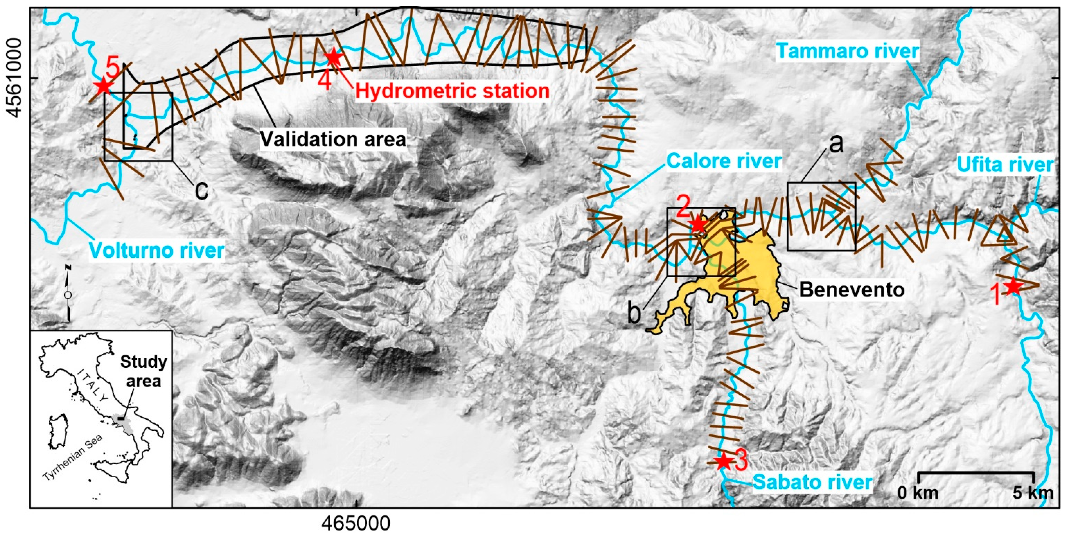
2. Study Area
3. Material and Methods
3.1. Materials
3.2. Nonstationary Frequency Analysis and Reference Flood Scenario
3.3. Flood Hazard Mapping Accounting for Multiple Probability Model
3.4. Validation
4. Results
4.1. Floods Probability
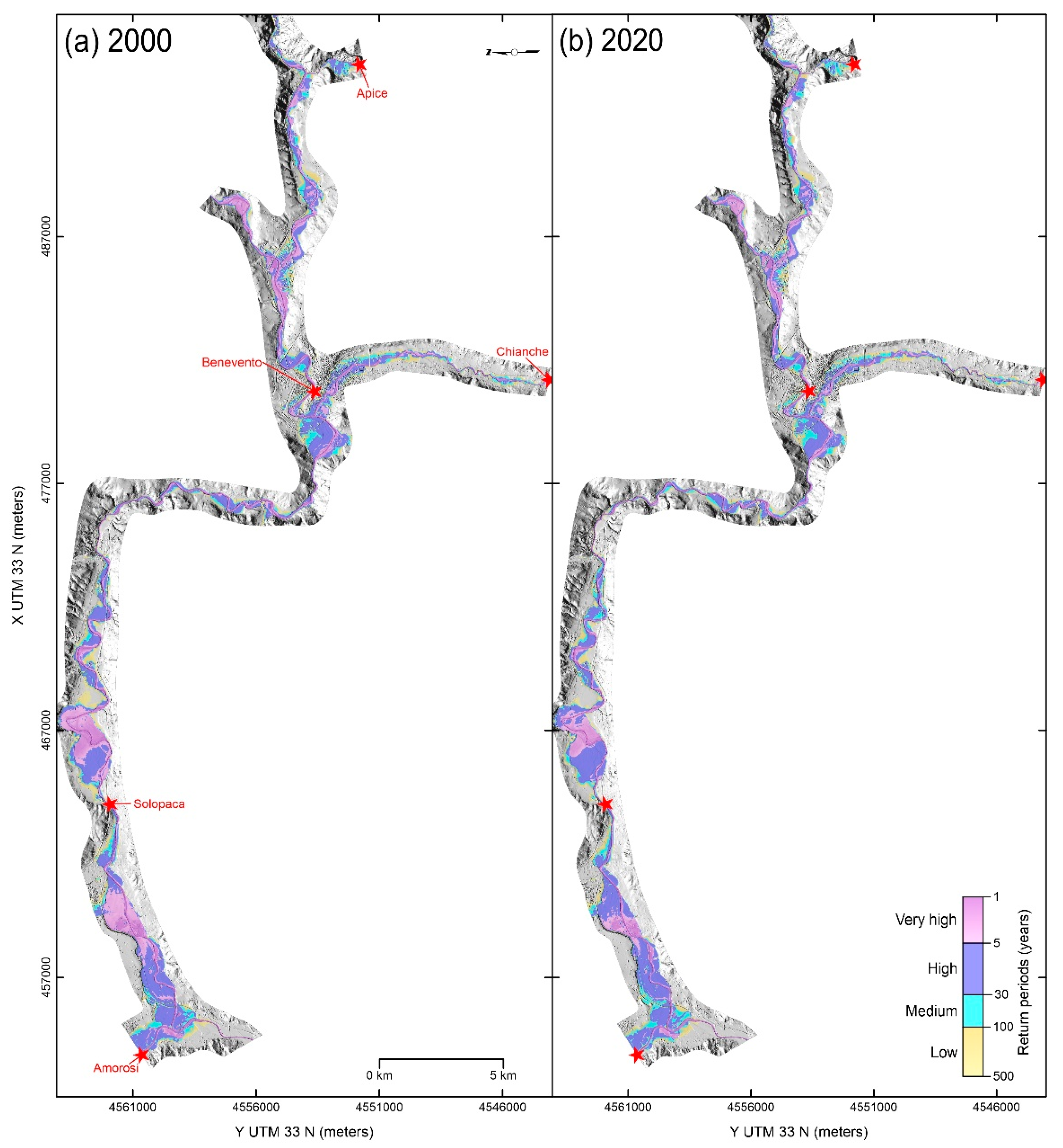
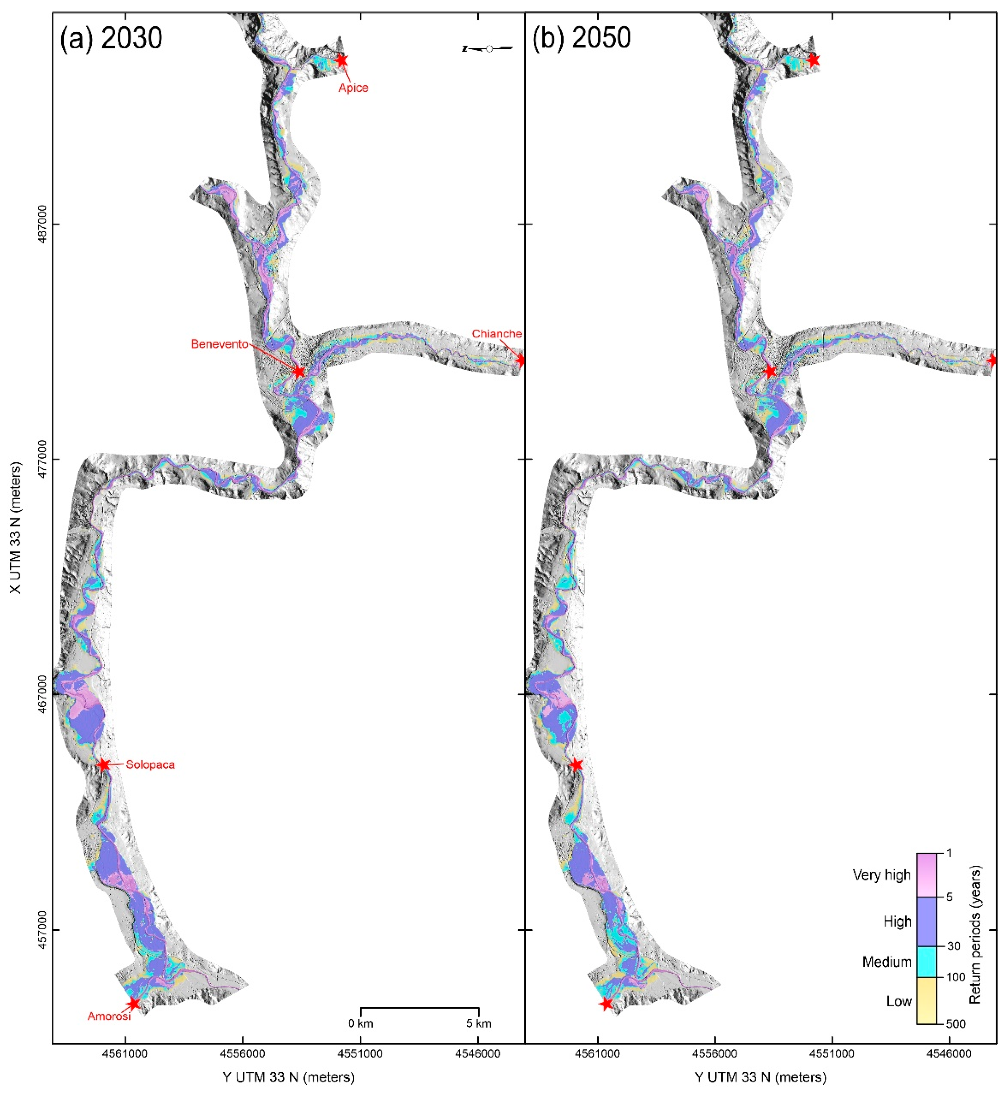
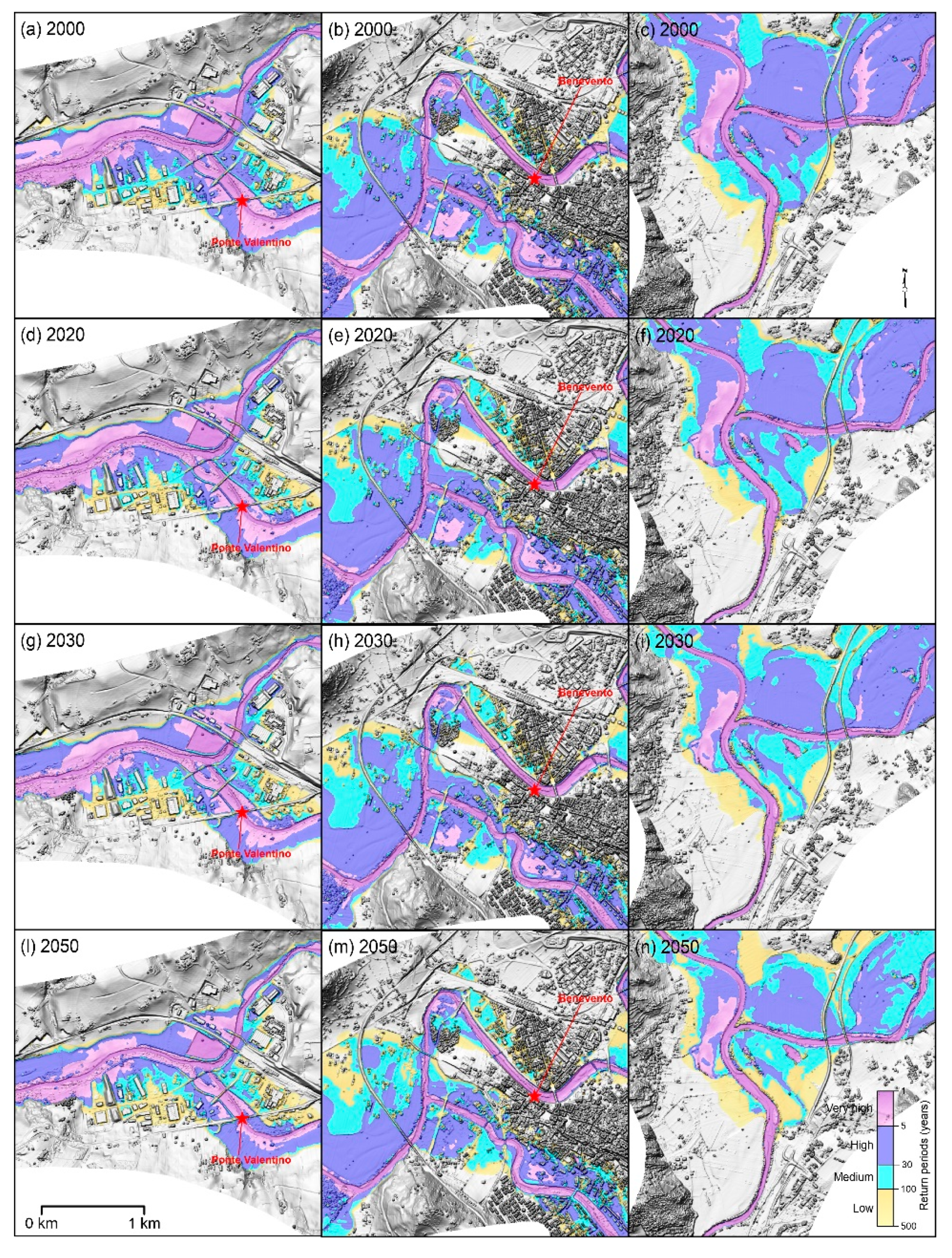
4.2. Maps Showing Flood Hazard Evolution
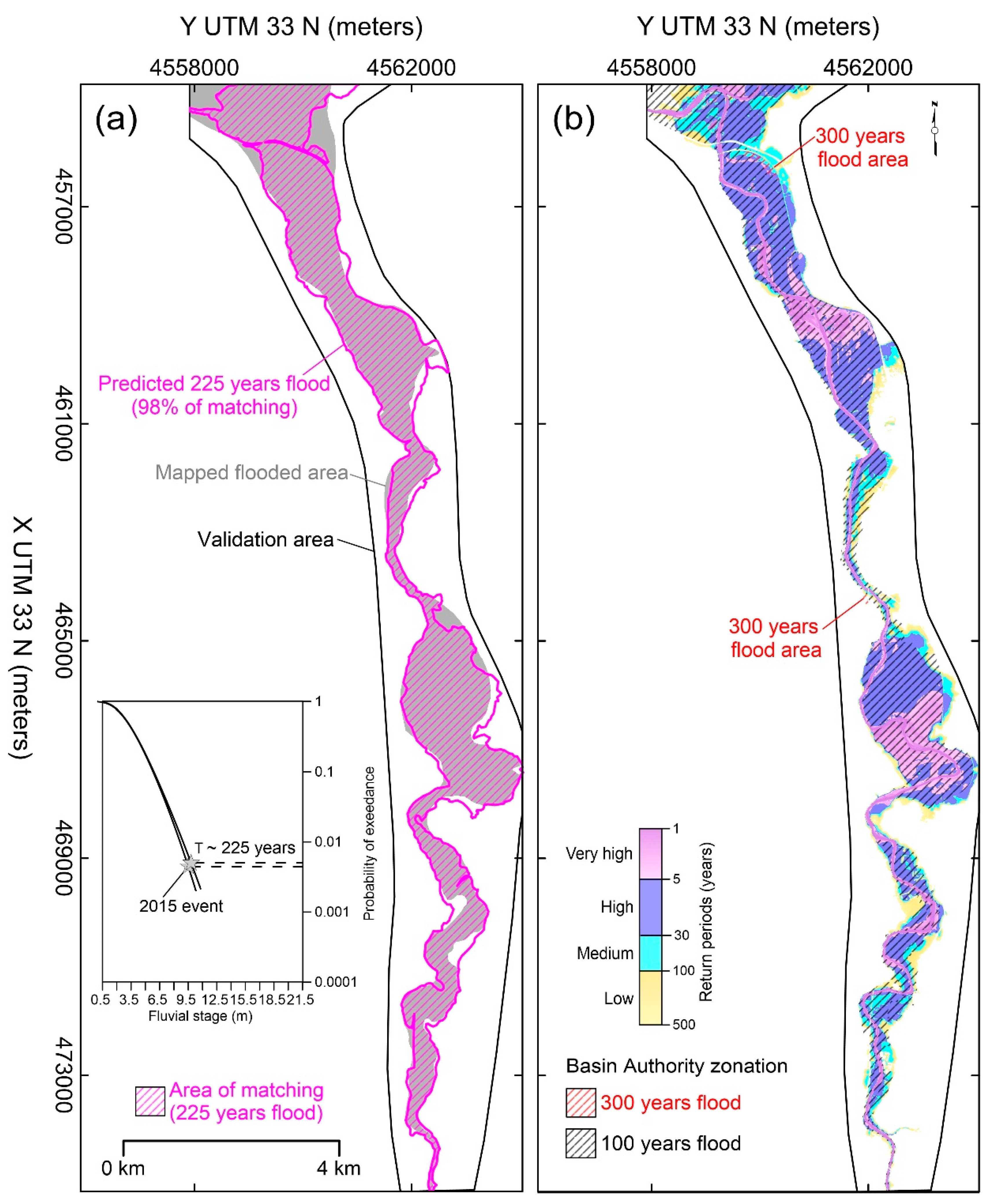
4.3. Validation
5. Discussion
6. Conclusions
Author Contributions
Funding
Acknowledgments
Conflicts of Interest
References
- Van Vliet, M.T.H.; Franssen, W.H.P.; Yearsley, J.R.; Ludwig, F.; Haddeland, I.; Lettenmaier, D.P.; Kabat, P. Global river discharge and water temperature under climate change. Glob. Environ. Chang. 2013, 23, 450–464. [Google Scholar] [CrossRef]
- Ma, H.; Yang, D.; Tan, S.K.; Gao, B.; Hu, Q. Impact of climate variability and human activity on streamflow decrease in the Miyun Reservoir Catchment. J. Hydrol. 2010, 389, 317–324. [Google Scholar] [CrossRef]
- Naik, P.K.; Jay, D.A. Distinguishing human and climate influences on the Columbia River: Changes in mean flow and sediment transport. J. Hydrol. 2011, 404, 259–277. [Google Scholar] [CrossRef]
- Zhai, R.; Tao, F. Contributions of climate change and human activities to runoff change in seven typical catchments across China. Sci. Total Environ. 2017, 605–606, 219–229. [Google Scholar] [CrossRef] [PubMed]
- Yang, Y.; Weng, B.; Man, Z.; Yua, Z.; Zhao, J. Analyzing the contributions of climate change and human activities on runoff in the Northeast Tibet Plateau. J. Hydrol. Reg. Stud. 2020, 27, 100639. [Google Scholar] [CrossRef]
- Xu, H.; Luo, Y. Climate change and its impacts on river discharge in two climate regions in China. Hydrol. Earth Syst. Sci. 2015, 19, 4609–4618. [Google Scholar] [CrossRef] [Green Version]
- Vogel, R.M.; Yaindl, C.; Walter, M. Nonstationarity: Flood magnification and recurrence reduction factors in the United States. J. Am. Water Resour. Assoc. 2011, 47, 464–474. [Google Scholar] [CrossRef]
- Ashraf, F.B.; Haghighi, A.T.; Marttila, H.; Kløve, B. Assessing impacts of climate change and river regulation on flow regimes in cold climate: A study of a pristine and a regulated river in the sub-arctic setting of Northern Europe. J. Hydrol. 2016, 542, 410–422. [Google Scholar] [CrossRef]
- Lobanova, A.; Liersch, S.; Nunes, J.P.; Didovets, I.; Stagl, J.; Huang, S.; Kocha, H.; Rivas López, M.R.; Maule, C.F.; Fred Hattermann, F.; et al. Hydrological impacts of moderate and high-end climate change across European river basins. J. Hydrol. 2018, 18, 15–30. [Google Scholar] [CrossRef]
- Billi, P.; Fazzini, M. Global change and river flow in Italy. Glob. Planet. Chang. 2017, 155, 234–246. [Google Scholar] [CrossRef]
- Knox, J.C. Large increase in flood magnitude in response to modest changes in climate. Nature 1993, 361, 430–432. [Google Scholar] [CrossRef]
- Hirabayashi, Y.; Mahendran, R.; Koirala, S.; Konoshima, L.; Yamazaki, D.; Watanabe, S.; Kim, H.; Kanae, S. Global flood risk under climate change. Nat. Clim. Chang. 2013, 3, 816–821. [Google Scholar] [CrossRef]
- Bangalore, M.; Smith, A.; Veldkamp, T. Exposure to Floods, Climate Change, and Poverty in Vietnam. Econ. Disasters Clim. Chang. 2019, 3, 79–99. [Google Scholar] [CrossRef] [Green Version]
- AghaKouchak, A.; Feldman, D.; Stewardson, M.J.; Saphores, J.D.; Grant, S.; Sanders, B.F. Australia’s drought: Lessons for california. Science 2014, 343, 1430–1431. [Google Scholar] [CrossRef] [Green Version]
- Zarch, M.A.A.; Sivakumara, B.; Sharma, A. Droughts in a warming climate: A global assessment of Standardized precipitation index (SPI) and Reconnaissance drought index (RDI). J. Hydrol. 2015, 526, 183–195. [Google Scholar] [CrossRef]
- Carrão, H.; Naumann, G.; Barbosa, P. Global projections of drought hazard in a warming climate: A prime for disaster risk managemen. Clim. Dyn. 2018, 50, 2137–2155. [Google Scholar] [CrossRef] [Green Version]
- Di Baldassarre, G.; Schumann, G.; Bates, P.D.; Freer, J.E.; Beven, K.J. Flood-plain mapping: A critical discussion of deterministic and probabilistic approaches. Hydrol. Sci. J. 2010, 55, 364–376. [Google Scholar] [CrossRef]
- De Risi, R.; Jalayer, F.; De Paola, F. Meso-scale hazard zoning of potentially flood prone areas. J. Hydrol. 2015, 527, 316–325. [Google Scholar] [CrossRef]
- Nuswantoro, R.; Diermanse, F.; Molkenthin, F. Probabilistic flood hazard maps for Jakarta derived from a stochastic rain-storm generator. J. Flood Risk Manag. 2016, 9, 105–124. [Google Scholar] [CrossRef]
- Gonçalves, P.; Marafuz, I.; Gomes, A. Flood hazard, Santa Cruz do Bispo Sector, Leça River, Portugal: A methodological contribution to improve land use planning. J. Maps 2015, 11, 760–771. [Google Scholar] [CrossRef] [Green Version]
- Teng, J.; Jakeman, A.J.; Vaze, J.; Croke, B.F.W.; Dutta, D.; Kim, S. Flood inundation modelling: A review of methods, recent advances and uncertainty analysis. Environ. Model. Softw. 2017, 90, 201–216. [Google Scholar] [CrossRef]
- Guerriero, L.; Focareta, M.; Fusco, G.; Rabuano, R.; Guadagno, F.M.; Revellino, P. Flood hazard of major river segments, Benevento Province, Southern Italy. J. Maps 2018, 14, 597–606. [Google Scholar] [CrossRef] [Green Version]
- Wang, Z.; Lai, C.; Chen, X.; Yang, B.; Zhao, S.; Bai, X. Flood hazard risk assessment model based on random forest. J. Hydrol. 2015, 527, 1130–1141. [Google Scholar] [CrossRef]
- Alfonso, L.; Mukolwem, M.M.; Di Baldassarre, G. Probabilistic flood maps to support decision-making: Mapping the value of information. Water Resour. Res. 2016, 52, 1026–1043. [Google Scholar] [CrossRef] [Green Version]
- Gado, T.A.; Nguyen, V.T.V. An at-site flood estimation method in the context of nonstationarity I. A simulation study. J. Hydrol. 2016, 535, 710–721. [Google Scholar] [CrossRef]
- Debele, S.E.; Strupczewski, W.B.; Bogdanowicz, E. A comparison of three approaches to non-stationary flood frequency analysis. Acta Geophys. 2017, 65, 863–883. [Google Scholar] [CrossRef]
- Guerriero, L.; Ruzza, G.; Guadagno, F.M.; Revellino, P. Flood hazard mapping incorporating multiple probability models. J. Hydrol. 2020, 587, 125020. [Google Scholar] [CrossRef]
- Montané, A.; Buffin-Bélanger, T.; Vinet, F.; Vento, O. Mapping extreme floods with numerical floodplain models (NFM) in France. Appl. Geogr. 2017, 80, 15–22. [Google Scholar] [CrossRef]
- O’Brien, N.L.; Burn, D.H. A nonstationary index-flood technique for estimating extreme quantiles for annual maximum streamflow. J. Hydrol. 2014, 519, 2040–2048. [Google Scholar] [CrossRef]
- Bayazit, M. Nonstationarity of hydrological records and recent trends in trend analysis: A state of the art review. Environ. Process. 2015, 2, 527–542. [Google Scholar] [CrossRef]
- Gado, T.A.; Nguyen, V.T.V. An at-site flood estimation method in the context of nonstationarity II. Statistical analysis of floods in Quebec. J. Hydrol. 2016, 535, 722–736. [Google Scholar] [CrossRef]
- Šraj, M.; Viglione, A.; Parajka, J.; Blöschl, G. The influence of non-stationarity in extreme hydrological events on flood frequency estimation. J. Hydrol. Hydromech. 2016, 64, 426–437. [Google Scholar] [CrossRef] [Green Version]
- Liu, S.; Huang, S.; Xie, Y.; Wang, H.; Leng, G.; Huang, Q.; Wei, X.; Wang, L. Identification of the Non-stationarity of Floods: Changing Patterns, Causes, and Implications. Water Resour. Manag. 2019, 33, 939–953. [Google Scholar] [CrossRef]
- Coles, S. An Introduction to Statistical Modelling of Extreme Values; Springer Series in Statistics; Springer: London, UK, 2001; ISBN 1-85233-459-2. [Google Scholar]
- Mentaschi, L.; Vousdoukas, M.; Voukouvalas, E.; Sartini, L.; Feyen, L.; Besio, G.; Alfieri, L. The transformed-stationary approach: A generic and simplified methodology for non-stationary extreme value analysis. Hydrol. Earth Syst. Sci. 2016, 20, 3527–3547. [Google Scholar] [CrossRef] [Green Version]
- Milly, P.C.D.; Betancourt, J.; Falkenmark, M.; Hirsch, R.M.; Kundzewicz, Z.W.; Lettenmaier, D.P.; Stouffer, R.J. Stationarity Is Dead: Whither Water Management. Science 2008, 319, 573–574. [Google Scholar] [CrossRef]
- Serinaldi, F.; Kilsby, C.G. Stationarity is undead: Uncertainty dominates the distribution of extremes. Adv. Water Resour. 2015, 77, 17–36. [Google Scholar] [CrossRef] [Green Version]
- Domeneghetti, A.; Carisi, F.; Castellarin, A.; Brath, A. Evolution of flood risk over large areas: Quantitative assessment for the Po river. J. Hydrol. 2015, 527, 809–823. [Google Scholar] [CrossRef]
- Santo, A.; Santangelo, N.; Forte, G.; De Falco, M. Post flash flood survey: The 14th and 15th October 2015 event in the Paupisi-Solopaca area (Southern Italy). J. Maps 2017, 13, 19–25. [Google Scholar] [CrossRef] [Green Version]
- Revellino, P.; Guerriero, L.; Mascellaro, N.; Fiorillo, F.; Grelle, G.; Ruzza, G.; Guadagno, F.M. Multiple Effects of Intense Meteorological Events in the Benevento Province, Southern Italy. Water 2019, 11, 1560. [Google Scholar] [CrossRef] [Green Version]
- Magliulo, P.; Valente, A. GIS-Based Geomorphological Map of the Calore River Floodplain Near Benevento (Southern Italy) Overflooded by the 15th October 2015 Event. Water 2020, 12, 148. [Google Scholar] [CrossRef] [Green Version]
- Hess, A.; Iyer, H.; Malm, W. Linear trend analysis: A comparison of methods. Atmos. Environ. 2001, 35, 5211–5222. [Google Scholar] [CrossRef]
- Kundzewicz, Z.W.; Robson, A.J. Change detection in hydrological records-a review of the methodology. Hydrol. Sci. J. 2004, 49, 7–19. [Google Scholar] [CrossRef]
- Hosking, J.R.M.; Wallis, J.R. The value of historical data in flood frequency analysis. Water Resour. Res. 1986, 22, 1606–1612. [Google Scholar] [CrossRef] [Green Version]
- Delgado, J.M.; Apel, H.; Merz, B. Flood trends and variability in the Mekong river. Hydrol. Earth Syst. Sci. 2010, 14, 407–418. [Google Scholar] [CrossRef] [Green Version]
- Gül, G.; Aşıkoğlu, Ö.; Gül, A.; Gülçem Yaşoğlu, F.; Benzeden, E. Nonstationarity in flood time series. J. Hydrol. Eng. 2014, 19, 1349–1360. [Google Scholar] [CrossRef]
- Merz, B.; Thieken, A.H. Separating natural and epistemic uncertainty in flood frequency analysis. J. Hydrol. 2005, 309, 114–132. [Google Scholar] [CrossRef]
- Merz, B.; Thieken, A.H. Flood risk curves and uncertainty bounds. Nat. Hazards 2009, 51, 437–458. [Google Scholar] [CrossRef]
- Woo, M.; Waylen, P.R. Probability studies of floods. Appl. Geogr. 1986, 6, 185–195. [Google Scholar] [CrossRef]
- Cook, A.; Merwade, V. Effect of topographic data, geometric configuration and modelling approach on flood inundation mapping. J. Hydrol. 2009, 377, 131–142. [Google Scholar] [CrossRef]
- Molinari, D.; De Bruijn, K.M.; Castillo-Rodríguez, J.T.; Aronica, G.T.; Bouwer, L.M. Validation of flood risk models: Current practice and possible improvements. Int. J. Disaster Risk Reduct. 2019, 33, 441–448. [Google Scholar] [CrossRef]
- Di Baldassarre, G.; Kooy, M.; Kemerink, J.S.; Brandimarte, L. Towards understanding the dynamic behavior of floodplains as human-water systems. Hydrol. Earth Syst. Sci. 2013, 17, 3235–3244. [Google Scholar] [CrossRef] [Green Version]
- Magliulo, P.; Valente, A.; Cartojan, E. Recent geomorphological changes of the middle and lower Calore River (Campania, Southern Italy). Environ. Earth Sci. 2013, 70, 2785–2805. [Google Scholar] [CrossRef]
- Matalas, N.C. Stochastic hydrology in the context of climate change. In Climate Change and Water Resources Planning Criteria; Frederick, K.D., Major, D.C., Stakhiv, E.Z., Eds.; Springer: New York, NY, USA, 1997; pp. 89–101. [Google Scholar]
- Gilroy, K.L.; McCuen, R.H. A nonstationary flood frequency analysis method to adjust for future climate change and urbanization. J. Hydrol. 2012, 414–415, 40–48. [Google Scholar] [CrossRef]
- Lima, C.H.R.; Lall, U.; Troy, T.J.; Devineni, N. A climate informed model for nonstationary flood risk prediction: Application to Negro River at Manaus, Amazonia. J. Hydrol. 2015, 522, 594–602. [Google Scholar] [CrossRef]
- Faulkner, D.; Warren, S.; Spencer, P.; Sharkey, P. Can we still predict the future from the past? Implementing non-stationary flood frequency analysis in the UK. J. Flood Risk Manag. 2020, 13, e12582. [Google Scholar] [CrossRef] [Green Version]
- Cohn, T.A.; Lins, H.F. Nature’s style: Naturally trendy. Geophys. Res. Lett. 2005, 32, L23402. [Google Scholar] [CrossRef] [Green Version]
- De Paola, F.; Giugni, M.; Pugliese, F.; Annis, A.; Nardi, F. GEV Parameter Estimation and Stationary vs. Non-Stationary Analysis of Extreme Rainfall in African Test Cities. Hydrology 2018, 5, 28. [Google Scholar] [CrossRef] [Green Version]
- Parkers, B.; Demeritt, D. Defining the hundred year flood: A Bayesian approach for using historic data to reduce uncertainty in flood frequency estimates. J. Hydrol. 2016, 540, 1189–1208. [Google Scholar] [CrossRef] [Green Version]
- Katz, R.W.; Parlange, M.B.; Naveau, P. Statistics of extremes in hydrology. Adv. Water Resour. 2002, 1287–1304, 8–12. [Google Scholar] [CrossRef] [Green Version]
- Brandt, S.; Lim, N. Importance of river bank floodplain slope in the accuracy of flood inundation mapping. River Flow 2012: Volume 2. In Proceedings of the International Conference of Fluvial Dynamics, San Jose, Costa Rica, 5–7 September 2012; CRC Press: Boca Raton, FL, USA; Taylor and Francis: Abingdon, UK, 2012; pp. 1015–1020. [Google Scholar]
- Ghizzoni, T.; Roth, G.; Rudari, R. Multisite flooding hazard assessment in the Upper Mississippi River. J. Hydrol. 2012, 412, 101–113. [Google Scholar] [CrossRef]
- Rojas, R.; Feyen, L.; Wathkiss, P. Climate change and river floods in the European Union: Socio-economic consequences and the costs and benefits of adaptation. Glob. Environ. Chang. 2013, 23, 1737–1751. [Google Scholar] [CrossRef]


| n° | Name | Installation Year | Sample Size | Trend | p-Value |
|---|---|---|---|---|---|
| 1 | Apice | 1935 | 53 | −0.015 (0.047) | 0.001 |
| 2 | Benevento | 1924 | 48 | −0.019 (0.007) | 0.1 |
| 3 | Chianche | 1967 | 42 | −0.025 (0.005) | 0.008 |
| 4 | Solopaca | 1957 | 53 | −0.040 (0.011) | 0.004 |
| 5 | Amorosi | 1935 | 68 | −0.010 (0.003) | 0.01 |
| n° | Station | σ | µ0 | µt | |
|---|---|---|---|---|---|
| 1 | Apice | −0.014 (0.075) | 0.798 (0.084) | 4.402 (0.247) | −0.015 (0.004) |
| 2 | Benevento | −0.075 (0.091) | 1.554 (0.174) | 4.320 (0.416) | −0.019 (0.007) |
| 3 | Chianche | +0.055 (0.093) | 0.533 (0.065) | 2.034 (0.168) | −0.025 (0.005) |
| 4 | Solopaca | −0.045 (0.095) | 1.521 (0.167) | 4.955 (0.411) | −0.040 (0.011) |
| 5 | Amorosi | −0.213 (0.120) | 0.804 (0.086) | 2.899 (0.210) | −0.010 (0.003) |
| Apice | Benevento | Chianche | Solopaca | Amorosi | |
|---|---|---|---|---|---|
| 2000 | 6.2 | 10.6 | 4.7 | 11.5 | 5 |
| 2020 | 5.9 | 10.2 | 4.6 | 10.6 | 4.8 |
| 2030 | 5.7 | 10 | 4.4 | 10.3 | 4.7 |
| 2050 | 4.4 | 9.7 | 3.9 | 9.5 | 4.5 |
© 2020 by the authors. Licensee MDPI, Basel, Switzerland. This article is an open access article distributed under the terms and conditions of the Creative Commons Attribution (CC BY) license (http://creativecommons.org/licenses/by/4.0/).
Share and Cite
Guerriero, L.; Ruzza, G.; Calcaterra, D.; Di Martire, D.; Guadagno, F.M.; Revellino, P. Modelling Prospective Flood Hazard in a Changing Climate, Benevento Province, Southern Italy. Water 2020, 12, 2405. https://0-doi-org.brum.beds.ac.uk/10.3390/w12092405
Guerriero L, Ruzza G, Calcaterra D, Di Martire D, Guadagno FM, Revellino P. Modelling Prospective Flood Hazard in a Changing Climate, Benevento Province, Southern Italy. Water. 2020; 12(9):2405. https://0-doi-org.brum.beds.ac.uk/10.3390/w12092405
Chicago/Turabian StyleGuerriero, Luigi, Giuseppe Ruzza, Domenico Calcaterra, Diego Di Martire, Francesco M. Guadagno, and Paola Revellino. 2020. "Modelling Prospective Flood Hazard in a Changing Climate, Benevento Province, Southern Italy" Water 12, no. 9: 2405. https://0-doi-org.brum.beds.ac.uk/10.3390/w12092405