Hazard Mapping of the Rainfall–Landslides Disaster Chain Based on GeoDetector and Bayesian Network Models in Shuicheng County, China

Abstract

Landslides are among the most frequent natural hazards in the world. Rainfall is an important triggering factor for landslides and is responsible for topples, slides, and debris flows—three of the most important types of landslides. However, several previous relevant research studies covered general landslides and neglected the rainfall–topples–slides–debris flows disaster chain. Since landslide hazard mapping (LHM) is a critical tool for disaster prevention and mitigation, this study aimed to build a GeoDetector and Bayesian network (BN) model framework for LHM in Shuicheng County, China, to address these geohazards. The GeoDetector model will be used to screen factors, eliminate redundant information, and discuss the interaction between elements, while the BN model will be used for constructing a causality disaster chain network to determine the probability and risk level of the three types of landslides. The practicability of the BN model was confirmed by error rate and scoring rules validation. The prediction accuracy results were tested using overall accuracy, Matthews correlation coefficient, relative operating characteristics curve, and seed cell area index. The proposed framework is demonstrated to be sufficiently accurate to construct the complex LHM. In summary, the combination of the GeoDetector and BN model is very promising for spatial prediction of landslides.

1. Introduction

Among the most frequent natural disasters, landslides often result in several casualties and huge economic losses, seriously affecting social development and land use [1,2]. In 2016, 9710 landslides occurred in China, causing 370 deaths and approximately USD 457 million in direct economic losses [3]. Topples, slides, and debris flows are the three most important types of landslides. Landslide hazard mapping (LHM) is an important tool for disaster prevention and mitigation because it can point out the vulnerable areas of landslides [4,5,6]. Hence, it is crucial to select suitable influencing factors and research methods to ensure the accuracy of the landslide hazard mapping and assessment.

A disaster chain is a series of secondary disasters caused by primary disasters [7] and can be divided into concurrent disaster chains and serial disaster chains, according to the chain characteristics [8]. Disaster chains have three distinct features: inducibility, timing property, and scalability. As a disaster chain shows a continuous trend of chain structure evolution, its damage and impact are far greater than individual disasters [9,10]. For landslides, rainfall is one of the most important triggering factors, especially short-term and instantaneous extreme rainfall [11,12,13]. The hazard assessment of topple, slide, and debris flow events triggered by the intensity, duration, and type of rainfall has long been a question of great interest in a wide range of fields [14,15,16,17].

Landslide susceptibility mapping (LSM) is the most common regional landslide prevention tool and has a very long research history. However, research methods are still being innovated. At the previous study, most of the traditional research is based on statistical methods, such as AHP [18], Frequency Ratio [19], Weight of Evidence [20], and Information Entropy. With the development of computer science, more and more machine learning models have been introduced into LSM research, such as Logistic Regression model [21]. Naive Bayes [22], Decision Tree [23], Support Vector Machines [24] Genetic Algorithm [25], Random Forests [26,27], and the latest very popular neural network models, including Artificial Neural Networks [28], Convolution Neural Networks [29], and Recurrent Neural Networks [30]. These models are based on using historical hazards data to obtain the relationship between the influencing factors and landslide hazards, predicting the probability of hazard event occurrence in the future, and draw the spatial distribution map.

There are few studies on risk assessment for a rainfall–landslides disaster chain, and the methods listed above do not fully reflect the structure and probability of the rainfall–landslides disaster chain. However, the Bayesian Network (BN) model can combine the probabilistic approach with a clear graph of causal relationships between variables. The BN model can also offer a framework for dealing with uncertainty and complexity in disaster chain systems [31]. Meanwhile, the GeoDetector model is a spatial statistical tool used to evaluate the relative importance of various influencing factors of landslides. It is also helpful in explaining the occurrence of landslides [32]. By using the GeoDetector model, we can screen the influencing factors and exclude redundant ones. Therefore, the GeoDetector and BN models can be combined to perform landslide hazard assessment.

In this study, we collected precipitation data, field survey data, and remote sensing interpretation data from Shuicheng County, China. Since rainfall is the main landslides triggering factor in the study area, we chose the rainfall–topples–slides–debris flows disaster chain as the research subject. A new framework based on the GeoDetector and BN models is proposed in this paper. It uses the GeoDetector model to select influencing factors, applies the BN model to predict the probability and risk level of three types of landslides under different conditions, and uses ArcGIS for spatial mapping. This framework is evaluated by the overall accuracy value (OA), Matthews correlation coefficient (MCC), relative operating characteristics (ROC) curve, and seed cell area index (SCAI). Finally, LHM construction is completed. The highlights of this paper include: different thresholds for rainfall factors are assigned to discriminate the daily rainfall thresholds that induce landslides in the study area by filtering the factors; the Geodetector model is used to analyze the landslide factors, including the single factor driven and factors interaction driven, so as to eliminate redundant factors. The BN model is used for modeling the causal network of the complex rainfall–landslide disaster chain and to construct the LHM.

2. Study Area and Data

2.1. Study Area

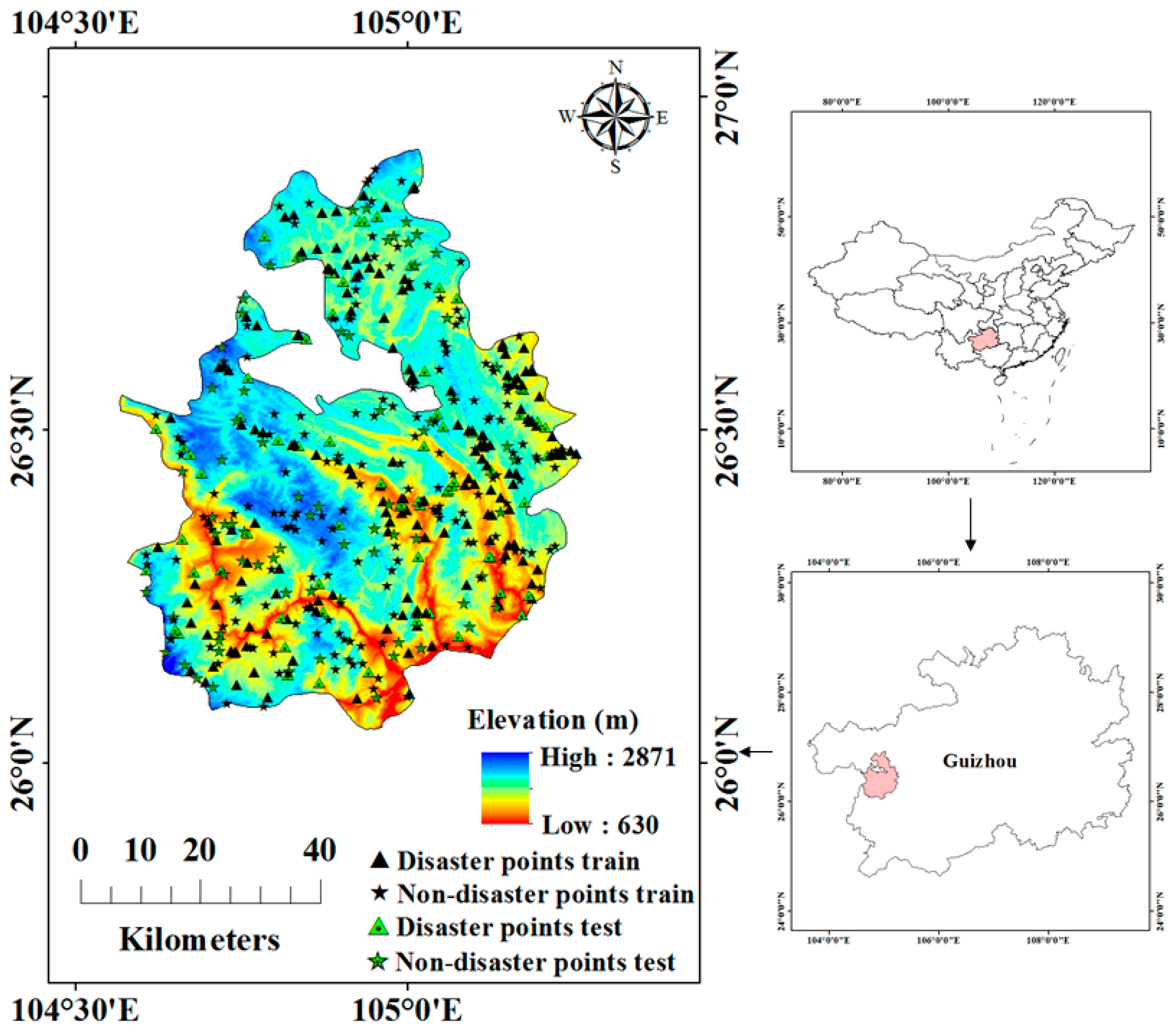
Shuicheng County is located in the Liupanshui Municipality, in western Guizhou Province, China. The area covers roughly 3605 km² and lies between longitudes 104°34′ E and 105°15′ E, and latitudes 26°03′ N and 26°55′ N, with a population of about 754,900 [33]. 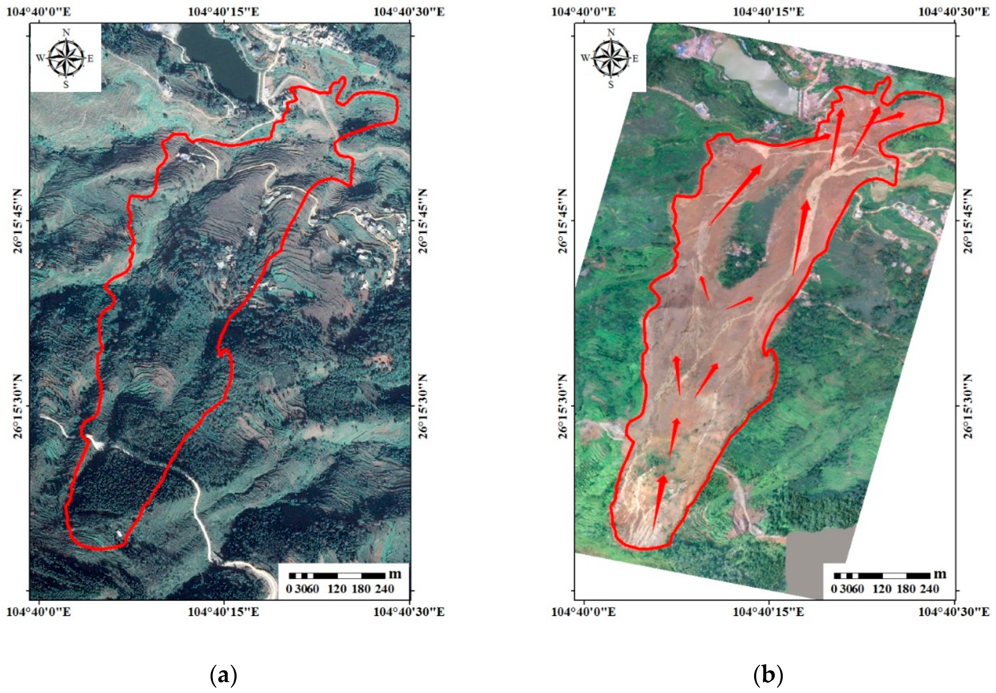In the study area, most of the slopes are very steep, with approximately 32.5% of the study area has slopes higher than 20° and large elevation fluctuations ranging from 630 m to 2871 m (Figure 1). Shuicheng County has a subtropical monsoon climate, with an annual sunshine duration of 1300–1500 h, annual average temperature of 12.4 °C, and annual average precipitation of about 1100 mm. The precipitation is heavy and frequent, mostly concentrated in summer, and often occurs in the form of torrential rain. In addition, the study area is a karst landscape, with surface water leaking in easily, and a high soil moisture content. According to historical statistics, there have been 240 topples, slides, and debris flows that occurred in Shuicheng County during 1999–2018 [34], which is a high-incidence area of concentrated landslides within China. On 23 July 2019, a huge landslide occurred in the town of Jichang in the study area, which destroyed houses, roads, and large areas of forest, caused 52 deaths and huge economic losses [35] (Figure 2). Hence, the assessment of landslide hazards in this study area is particularly important.

2.2. Landslides Inventory

The landslides inventory in Shuicheng County were monitored using field survey and remote sensing images. The landslides inventory map displays 240 historical disaster points, with loss data from each disaster provided by the China Geological Survey [34]. These points are the centroid of landslide scarp, which has been proved the best landslide sampling strategy [36], and they were derived from latitude and longitude vectoring combining remote sensing imagery and field surveys. We extracted 45 topple points, 155 slide points, and 40 debris flow points from the landslides inventory and classified each hazard into 5 risk levels according to the loss. Based on the disaster chain, we considered the slide to also be the topple, and the debris flow is both topple and slide. Finally, we got 240 topple points, 195 slide points, and 40 debris flow points. All the disaster points were used to construct a dataset. The landslides inventory map is shown in Figure 1.

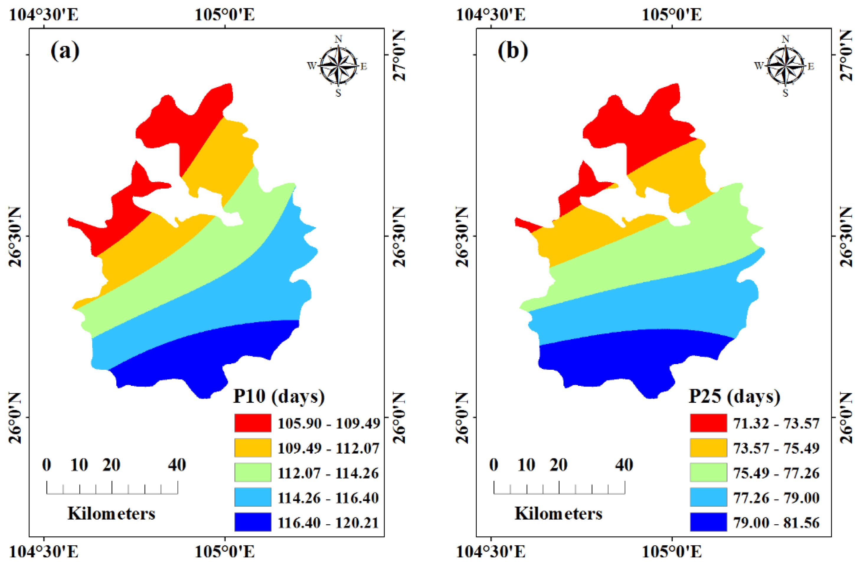
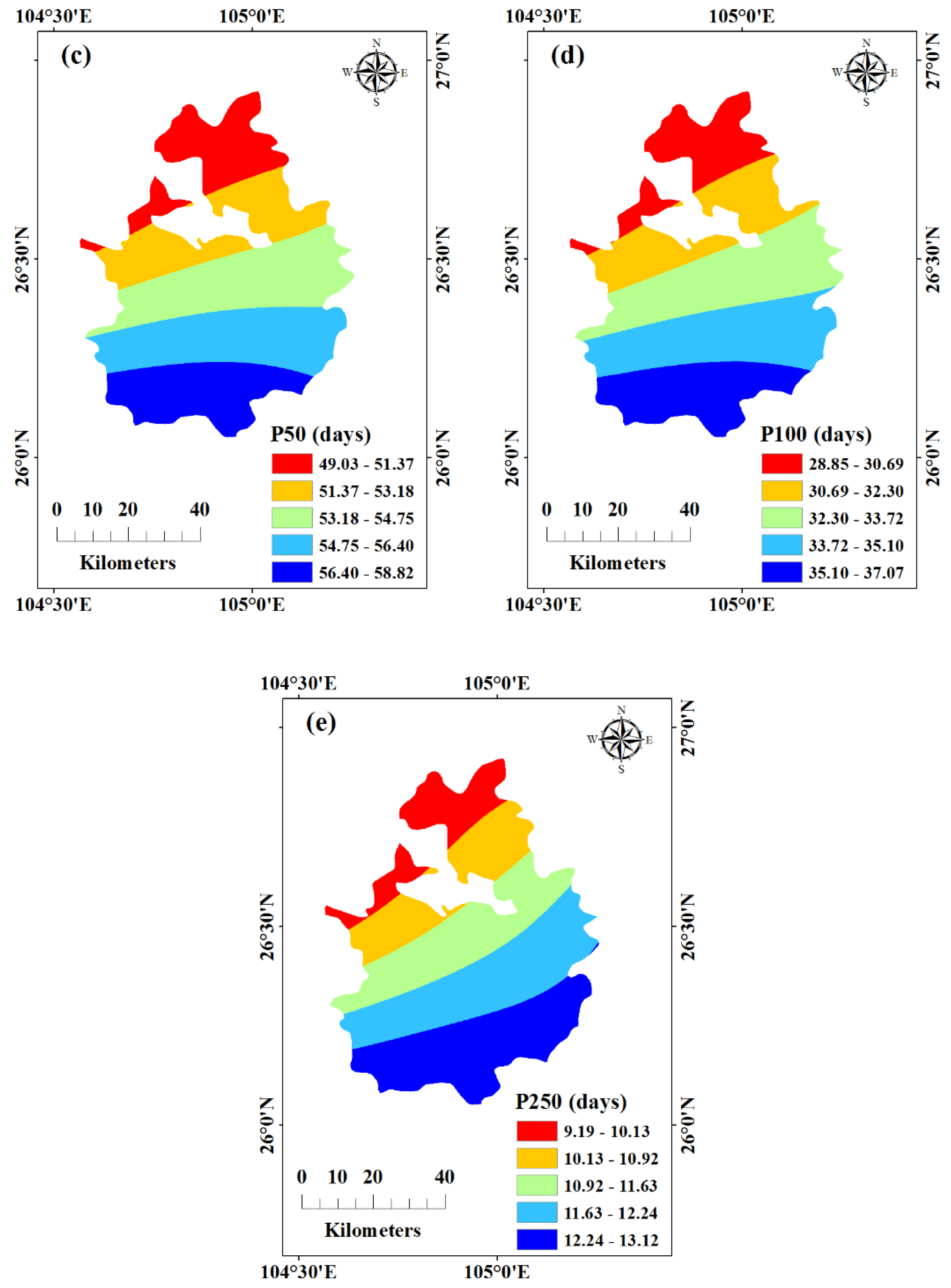
2.3. Extreme Rainfall Factors

In the disaster chain of rainfall–landslides, extreme rainfall is the primary trigger. To measure the influence of different rainfall intensities on the spatial distribution of landslides, five rainfall factors were established in this study, as listed in

Table 1. Extreme rainfall factors and intensity grade.

Extreme Rainfall Factors	24 h Rainfall	Rainfall Intensity Grade
P10	>10 mm	Above moderate rain
P25	>25 mm	Above heavy rain
P50	>50 mm	Above rainstorm
P100	>100 mm	Above heavy rainstorm
P250	>250 mm	Above torrential rainstorm

.

Daily precipitation data for 7 meteorological stations around the study area during the 1981–2018 timeframe were obtained from the China Meteorological Information Center [37]. We calculated the extreme rainfall factor values of each meteorological station, and the calculation formula is as follows:

$$P_i=\frac{1}{38}{\displaystyle \sum _{a=1}^{38}}{\displaystyle \sum _{d=1}^{365}}{C}_d$$

(1)

$$C_d=\{\begin{array}{c}1,\hspace{1em}{\mathrm{R}}_d>{\mathrm{R}}_i\\ 0,\hspace{1em}{\mathrm{R}}_d<{\mathrm{R}}_i\end{array}$$

(2)

where $P_i$ is the value of extreme rainfall factor $i$, which can be defined as the annual average number of days of rainfall above the threshold, $a$ represents the year, $d$ the date, ${\mathrm{R}}_d$ the $d$ day rainfall, and ${\mathrm{R}}_i$ the rainfall threshold of the rainfall factor $i$.

The spatial interpolation of rainfall factors at various points was carried out by Inverse Distance Weight (IDW) and used to obtain the continuous distribution data of each rainfall factor (Figure 3).

2.4. landslides Influencing Factors

The conditions influencing the factors of landslides are crucial for determining a landslide hazard assessment. Historical disaster points were used to establish LHM methods because of the supposition that future landslide events will occur under the same or similar environmental conditions as previous hazards [29]. There are approximately 100 influencing factors affecting the occurrence of landslides [38]. Therefore, it is crucial to select suitable influencing factors to draw LHM with sufficient precision [39,40].

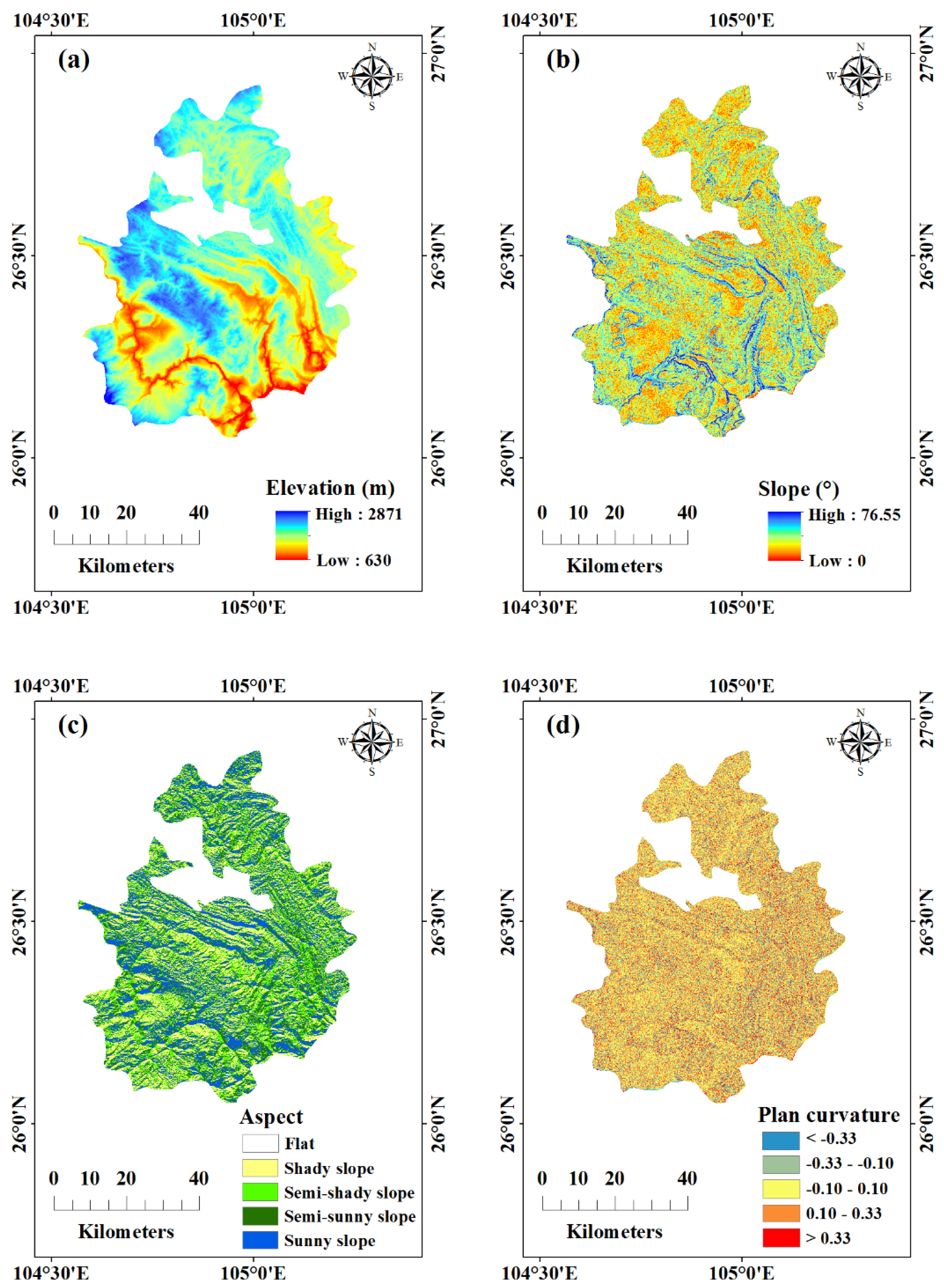
In this study, 11 influencing factors were selected due to the close relationship between these factors and landslides (

Table 2. The names, data structures, variable types, and data descriptions of landslide hazard influencing factors.

Name	Data Structure	Variable Type	Data Description
Elevation	Raster	Continuous	Height above sea level
Slope	Raster	Continuous	Extracted from DEM
Aspect	Raster	Discrete	Extracted from DEM
Plan curvature	Raster	Discrete	Extracted from DEM
Profile curvature	Raster	Discrete	Extracted from DEM
Lithology	Polygon	Discrete	Digitized from geological map
Geological age	Polygon	Discrete	Digitized from geological map
Faults	Line	Continuous	Distance to faults
Rivers	Line	Continuous	Distance to rivers
Roads	Line	Continuous	Distance to roads
NDVI	Raster	Continuous	The vegetation of land cover

). We input these influencing factors into a uniform format database, according to the Digital Elevation Model (DEM) map pixel size. All of the factors’ pixel sizes were set to 30 × 30 m using the Fishnet tool in ArcGIS 10.6, regardless of the initial data format.

Among the influencing factors, topography has an extremely important influence on the soil moisture and groundwater and influences slope stabilities [1]. In this study, DEM with a 30 × 30 m pixel size was used from Advanced Spaceborne Thermal Emission and Reflection Radiometer Digital Elevation Model (ASTER DEM) data jointly developed by METI, Japan, and NASA, the USA provided by the Geospatial Data Cloud site, Computer Network Information Center, Chinese Academy of Sciences in 2019 [41]. Elevation, slope, aspect, plan curvature, and profile curvature data were extracted from DEM.

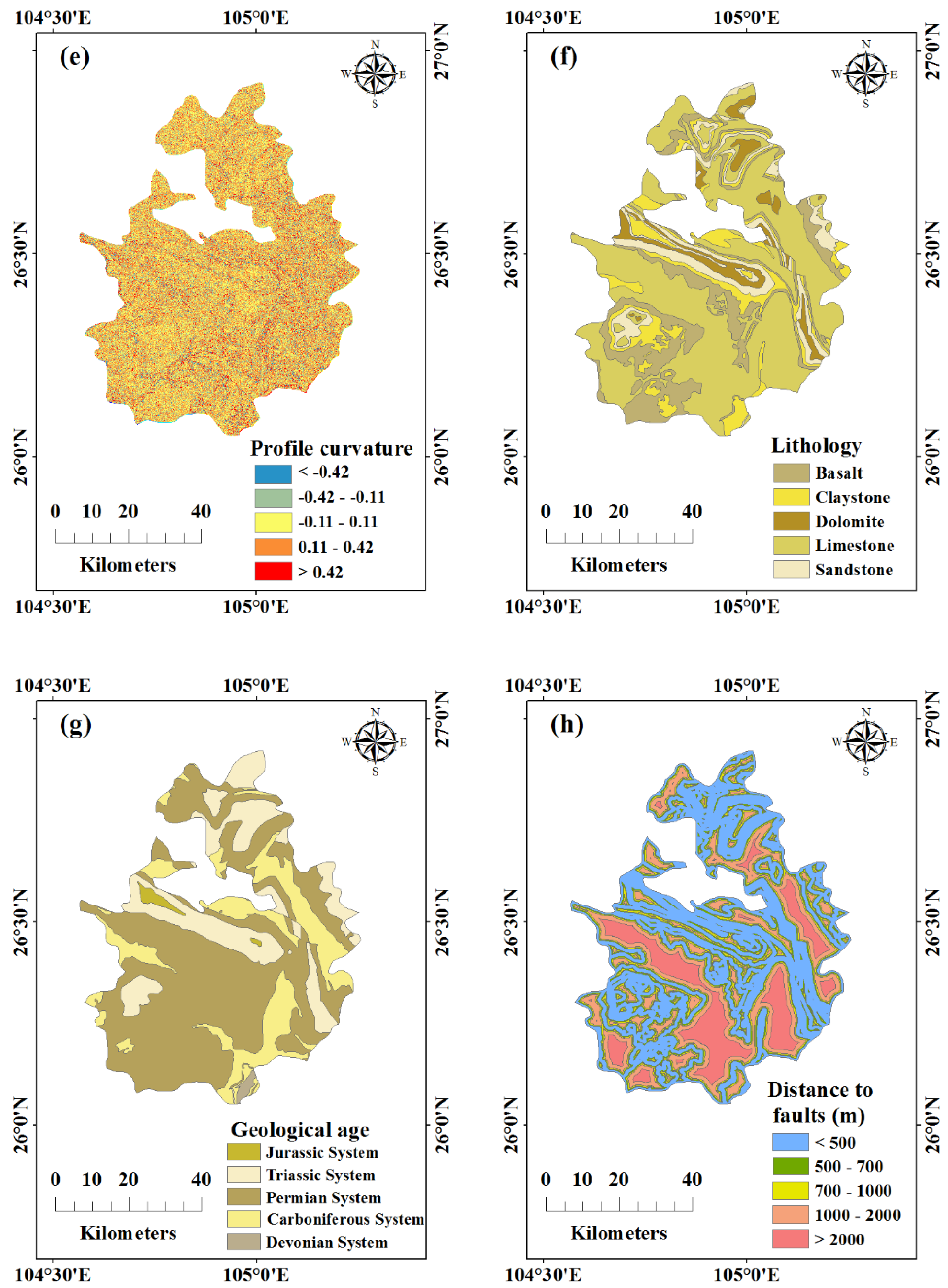
Lithology is one of the most important influencing factors in landslide hazard mapping [42]. Geological age can characterize the development of regional lithology to a certain extent; thus, it was also analyzed as an alternative factor in our study. Faults control the formation and development of landslides, and geological processes are more active in the vicinity of faults. The lithology and geological age are polygon vector maps that were digitized from geological maps obtained from the China Geology Survey in 2019. We then received the lithology and geological age data, and were able to calculate the distance to faults.

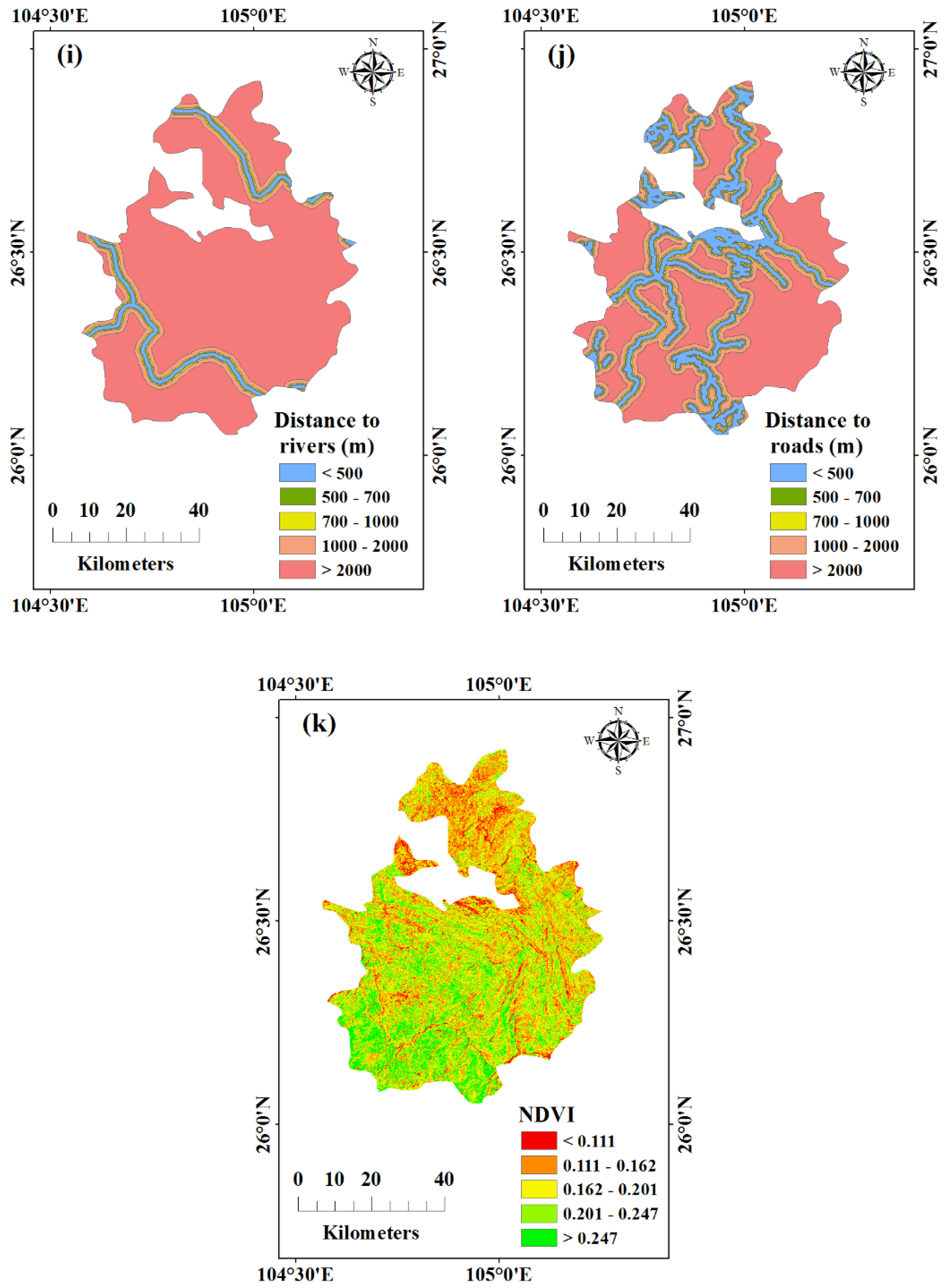
Hydrology is another important factor in the formation of landslides [43]. Surface rivers are among the most active factors in external dynamic geology. The closer the surface is to the river, the more serious is the occurrence of scours at the foot of the slope, providing favorable conditions for landslides to occur. The rivers map is a polyline vector which was interpreted on Google Earth in 2018.

Roads can also reflect the possible influence of human activities on landslides to a certain extent. Meanwhile, the traffic on roads can cause vibrations to destabilize rock material. The closer the distance to the road, the higher is the possibility that landslides will occur. Therefore, we selected the distance from the road as one of the initial influencing factors of LHM. The roads map is a polyline vector that was also interpreted on Google Earth in 2018.

Land cover is often selected as a factor in landslides research, particularly vegetation cover, which has an important influence on slope stability [44]. Hence, we chose the normalized difference vegetation index (NDVI) to characterize land cover [45]. The NDVI data were calculated through Landsat 8 Operational Land Imager satellite remote sensing digital products with a pixel size of 30 × 30 m shot in April 2018 [46], using the band algebra tool of ENVI 5.3.

Maps of these influencing factors were shown in Figure 4.

3. Methods

The LHM process can be divided into three steps as follows. The first step is to choose both the triggering and influencing factors using the GeoDetector model. The second step is the classification between the two models, Geodetector and BN, of the disaster points into three types: topples, slides, and debris flows. Combining the factors selected by the GeoDetector model in the first step, these factors and the three types of landslides inventory layers were divided into grids, and their attribute tables were extracted and separated randomly to build the training sets and verification sets. The third step is running the model, including model training, model validation, and LHM mapping.

3.1. Data Pretreatment

First, we divided the study area into 30 × 30 m grids. A total of 4,321,030 grids were generated in the study area. Since there are no grids with more than two disaster points at the same time, each landslide grid was counted as 1, or as 0 if it includes no hazard. The type and risk level of each disaster point were also recorded in the attribute table. Since the GeoDetector and BN models specify that the factors entered must be partitioned data, in this study, we divided each factor into five grades, where continuous variables were reclassified using natural fracture methods such as the rainfall factors and elevation. In addition, the slope was classified into sunny slope (135–225°), semi-sunny slope (90–135°, 225–270°), semi-shady slope (45–90°, 270–315°), shady slope (0–45°, 315–360°), and flat slope according to the four direction method. For lithology, limestone, dolomite, sandstone, basalt, and claystone were classified into five groups. Then, the group of grids for each factor was used as the input data to carry out the calculation of the GeoDetector model and the construction of the BN model.

3.2. GeoDetector Model

The GeoDetector model is based on the geospatial differentiation theory and distinguishes the relationship between spatial zoning and changes in geographical phenomena of various influencing factors. The model also analyzes the mechanism behind this phenomenon, thereby detecting the different consequences of the influencing factors that determine the geographical phenomenon [47,48]. The core hypothesis of GeoDetector is that if an independent variable has an important influence on a dependent variable, the spatial distributions of the independent variable and the dependent variable should be similar [21,49]. The GeoDetector model software can be freely downloaded from http://www.geodetector.cn [50]. This model includes single factor driven analysis and two factor interaction driven analysis.

(1)

Single factor driven analysis. The GeoDetector quantitatively determines the contribution of the independent variable x to the dependent variable y by factor explanatory power, thereby checking whether the factor is the reason for the spatial differentiation of the geographical phenomenon. The principle of factor explanatory power is as follows:

$$q=1-\frac{1}{N{\sigma }^2}{\displaystyle {\sum }_{h=1}^L}{N}_h{\sigma }_h^2, q\in \left[0,1\right]$$

(3)

where $q$ is the factor explanatory power, indicating to what extent the independent variable explains the spatial distribution of landslides; $h=1,\dots ,\mathrm{L},$ is the count of independent variable class, $N_h$ and $N$ are the grids number of class $h$ and the whole area, respectively. ${\sigma }_h^2$ and ${\sigma }^2$ are the variance of the dependent variable of the class $h$ and whole area, respectively. The larger the values of $q$ become, the greater the contribution of the x-layer to landslides occurrence.

(2)

Factors interaction driven analysis. The interaction detector compares the explanatory power of the pairwise factors and their sum with the explanatory power after the interaction, to analyze the influence form of the two factors coincidence on the geographical phenomenon. X1 and X2 are two factors, spatially superposed X1 and X2 form a new spatial factor X1 ∩ X2, then we compare the interaction relationship between the factor explanatory power of X1 ∩ X2 and X1, X2.

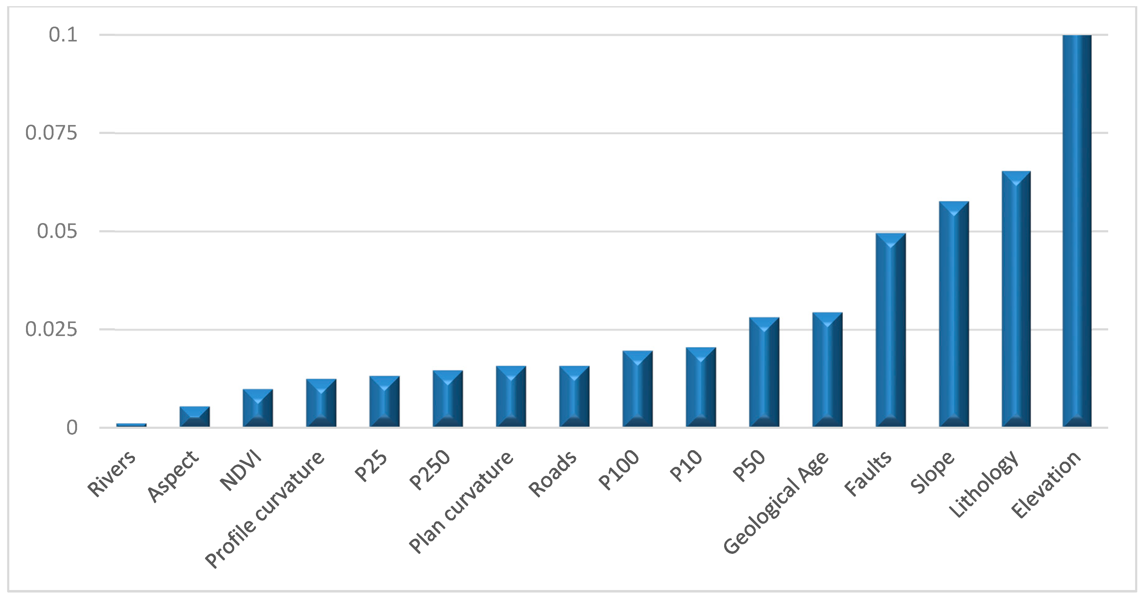
In this study, all 240 disaster points and an equal number of random non-disaster point grids were selected. Then, the attribute tables of selected grids were exported as input datasets to the GeoDetector model to calculate the explanatory power of all factors (Figure 5). Six factors with an explanatory power greater than 0.025 in single factor driven analysis were selected as independent variables in the LHM and applied to construct the BN model next.

3.3. BN Model

BN model is a very effective tool to model a complex causal network system [51]. It can intuitively represent the joint probability distribution of variables and their conditional independence by using a graphical network structure, which can save a lot of probabilistic reasoning calculation and can be very useful for probabilistic reasoning. BN is a directed acyclic graph (DAG) that includes a series of nodes, arcs, and conditional probability tables (CPTs) to indicate the joint probability distributions among the node factors [52,53]. These nodes can be classified into parent nodes and child nodes, which represent the inducing factors and the consequences of the variable, respectively. BN models can simply calculate the joint probability distributions. If the probability of the variable $X_i$’s parent node is defined as $P_a\left(X_i\right)$, the joint probability distribution $P_a\left(X_i\right)$ is expressed as follows [54]:

$$P\left(X\right)=P\left(X_1,X_2,\dots ,X_n\right)={\displaystyle {\prod }_{i=1}^n}P\left(X_i|P_a\left(X_i\right)\right), \left(i=1,2,\dots ,n\right)$$

(4)

in this formula, $X=\left(X_1,X_2,\dots ,X_n\right)$ represents the factors for different nodes, and $n$ is the number of factors.

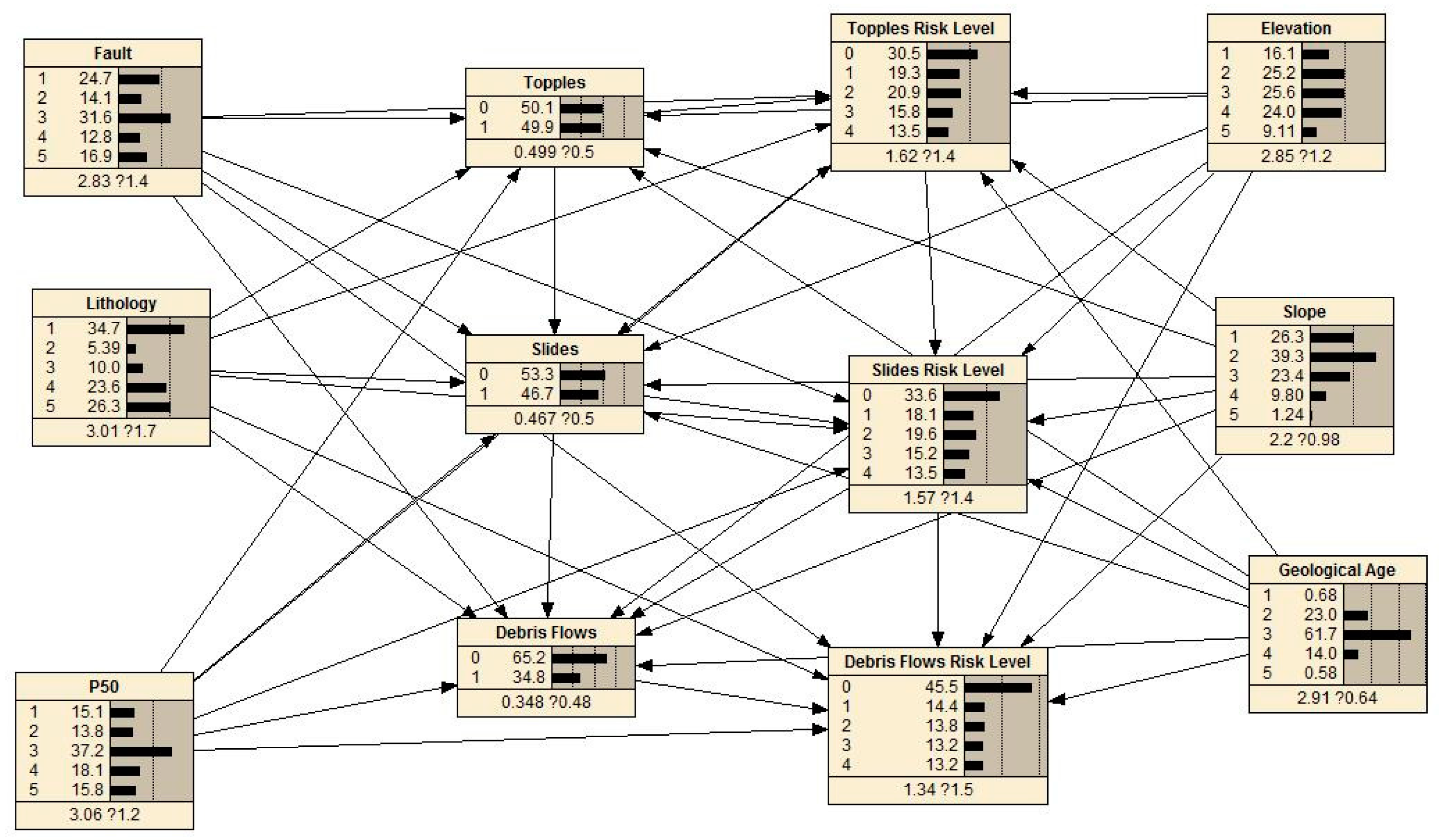
In this study, the occurrence and loss intensity of topples, slides, and debris flows in disaster chain are reflected as variables with their parent nodes and child nodes. When the occurrence of a type of landslides is the variable, its parent nodes include the extreme rainfall factors, influencing factors, as well as the primary type of landslides on the disaster chain; its child nodes include the casualty and property loss caused by the initial disaster and second type of landslides on the chain, combined with the appropriate factors selected by GeoDetector model. Finally, the BN model of the rainfall–topples–slides–debris flows disaster chain was constructed as shown in Figure 6.

In this study, 70% of each landslides type’s data set was randomly selected as a training set, and the remaining 30% of the disaster points were the verification set. The location of the training set and test set samples was shown in Figure 1, and the statistics of disaster points and non-disaster points were listed in

Table 3. Statistics of training set and test set samples.

	Training Set	Test Set
Topples	168	72
Slides	136	59
Debris flows	29	11
Non-topples	168	72
Non-slides	200	85
Non-debris flows	307	133

. By using Netica 5.18, which is a widely used Bayesian network development software and can be downloaded at https://www.norsys.com [55], we constructed the BN model, using the gradient ascent to learn the training set. The logarithmic loss, quadratic loss, and spherical payoff contained in the software were selected to preliminarily evaluate the error rate and scoring rules of the model [56]. The closer to zero for both logarithmic and quadratic loss, and the closer to 1 for the spherical payoff, the higher the accuracy of the model.

Table 4. Confusion matrix, error rate, and scoring rules of BN model.

Topples
Predicted				Actual		Error rate			0.1806
						Logarithmic loss			0.5180
Yes		No				Quadratic loss			0.2508
57		15		Yes		Spherical payoff			0.8589
11		61		No		Area under ROC			0.9105
Topples Risk Level
Predicted							Actual	Error rate	0.2639
Very Low	Low		Medium	High	Very High			Logarithmic loss	0.7157
64	4		2	2	0		Very Low
8	21		3	1	0		Low	Quadratic loss	0.3522
0	3		15	1	0		Medium
2	1		2	5	1		High	Spherical payoff	0.7914
0	0		0	0	1		Very High
Slides
Predicted				Actual		Error rate			0.1944
						Logarithmic loss			0.6005
Yes		No				Quadratic loss			0.2870
40		19		Yes		Spherical payoff			0.8407
9		76		No		Area under ROC			0.8791
Slides Risk Level
Predicted							Actual	Error rate	0.2639
Very Low	Low		Medium	High	Very High			Logarithmic loss	0.7561
78	3		2	1	1		Very Low
9	16		2	1	0		Low	Quadratic loss	0.3598
9	3		9	1	0		Medium
4	0		2	2	0		High	Spherical payoff	0.7911
0	0		0	0	1		Very High
Debris Flows
Predicted				Actual		Error rate			0.0625
						Logarithmic loss			0.2069
Yes		No				Quadratic loss			0.1055
4		7		Yes		Spherical payoff			0.9425
2		131		No		Area under ROC			0.8906
Debris Flows Risk Level
Predicted							Actual	Error rate	0.0625
Very Low	Low		Medium	High	Very High			Logarithmic loss	0.2098
131	1		1	0	0		Very Low
7	3		0	2	0		Low	Quadratic loss	0.1057
0	0		1	0	0		Medium
0	0		0	0	0		High	Spherical payoff	0.9425
0	0		0	0	0		Very High

lists the results of the confusion matrix, error rate, and scoring rules of the BN model.

According to the calculation results of the BN model and the level of the factors of each grid, we used MATLAB 2018b to write the model results into the attribute table of each grid; we then utilized ArcGIS 10.6 to map the spatial distribution of the possibility and the level of disaster loss of topples, slides, and debris flows. Based on the comprehensive evaluation of the three types of landslide hazards, we defined the hazard formula for the landslides:

$$H=P_C\times R_C+P_L\times R_L+P_D\times R_D$$

(5)

where $H$ is the hazard index of landslide hazard, $P_C$, $P_L$, $P_D$ are the possibilities of topples, slides, and debris flows, and $R_C$, $R_L$ $R_D$ are the risk level caused by topples, slides, and debris flows, respectively.

3.4. Model Evaluation

To evaluate the accuracy of this model, we selected the OA, MCC, and ROC curve methods to verify the accuracy of the model. The OA value is the proportion of the correctly classified grids to the total grids [57]:

$$\mathrm{OA}=\frac{a}{b}\times 100\%$$

(6)

where $a$ is the number of correctly classified grids, and $b$ is the number of total grids, respectively. The higher the OA value indicates the model is more accurate.

MCC is an index used to measure the performance of binary classifications in machine learning, which was first introduced from the biochemistry research field [58]. It considers true positive (TP), true negative (TN), false positive (FP), and false negative (FN). It can be applied even when the number of the two types of samples is very different. The MCC formula is as follows:

$$\mathrm{MCC}=\frac{\mathrm{TP}\times \mathrm{TN}-\mathrm{FP}\times \mathrm{FN}}{\sqrt{\left(\mathrm{TP}+\mathrm{FP}\right)\left(\mathrm{TP}+\mathrm{FN}\right)\left(\mathrm{TN}+\mathrm{FP}\right)\left(\mathrm{TN}+\mathrm{FN}\right)}}$$

(7)

The value of MCC ranges from −1 to 1, equal to 1 indicates the perfect prediction. When the MCC value equals 0, the prediction result is worse than random prediction. When it equals −1, the prediction result is completely inconsistent with the facts.

The ROC curve is the standard and most common method used to evaluate the performance of the landslide hazard prediction model [59,60]. It is plotted by the “Sensitivity” against the “1—Specificity” in statistics. The sensitivity and specificity are calculated as follow:

$$Sensitivity=\frac{\mathrm{TP}}{\mathrm{TP}+\mathrm{FN}}$$

(8)

$$Specificity=\frac{\mathrm{TN}}{\mathrm{TN}+\mathrm{FP}}$$

(9)

The area under the curve (AUC) is used to represent the accuracy of the assessment method [61], with values ranging from 0.5 to 1.0. AUC values closer to 1 indicate the model is more accurate [1,62].

Moreover, we used the SCAI method to analyze the accuracy of the model. This method can show the density of disaster chains among the classes [63]. The higher classes should have low values, while lower classes should have higher values if the model is accurate. The SCAI value is as follows:

$$SCA{I}_i=\frac{P_{ai}}{P_{di}}$$

(10)

In this formula, $i$ is the class of hazard, $P_{ai}$ is the percentage of class $i$ area in the total area, and $P_{di}$ is the proportion of class $i$ disaster points to total disaster points.

In the preliminary evaluation of the BN model, error rate equivalents to OA and Area under ROC equivalents to AUC. Logarithmic loss quantifies the classifier’s accuracy by penalizing misclassification, and it can be calculated as follow:

$$L\left(Y,P\left(\left(Y|X\right)\right)\right)=\frac{1}{N}{\displaystyle \sum _{i=1}^N}{\displaystyle \sum _{j=1}^M}{y}_{ij}log\left(p_{ij}\right)$$

(11)

where $Y$ is the output variable, $X$ is the input variable, and $L$ is the loss function. $N$ is the input sample size, $M$ is the number of possible categories, and $y_{ij}$ is a binary indicator of whether category $j$ is the true category of the input instance $x_i$. $P_{ij}$ is the probability that the model or classifier will predict that the input instance $x_i$ belongs to category $j$.

Quadratic loss is the square of the difference between the predicted value and the actual value:

$$L\left(y,f\left(x\right)\right)={\left(y-f\left(x\right)\right)}^2$$

(12)

where $y$ is the actual value and $f\left(x\right)$ is the predicted value.

Values of spherical payoff vary in the interval [0,1], with 1 being the best model performance, and is calculated as [64]:

$$\mathrm{MOAC}=\frac{P_c}{\sqrt{{\displaystyle {\sum }_{j=1}^n}{P}_j^2}}$$

(13)

where $\mathrm{MOAC}$ is the mean probability value of a given state averaged over all cases, $P_c$ is the probability predicted for the correct state, $P_j$ is the probability predicted for state $j$, and $n$ is the number of states.

4. Results

4.1. Single Factor Driven Analysis

The factors we used to interpret landslide hazards include elevation, lithology, and slope (Figure 5), which indicate that the occurrence of landslides is most closely related to these factors. Among the five rainfall factors, P50 has the maximum q-statistic value, indicating that daily rainfall over 50 mm has the most significant correlation with the spatial heterogeneity of landslides; 50 mm is also the most likely rainfall threshold to induce landslides in Shuicheng County. The explanatory power of aspect and distance to rivers is very small, meaning a very low relationship with the occurrence of landslides in the study area. As a result, we selected 0.025 as the threshold of explanatory power, and elevation, lithology, slope, distance to faults, geological age, and P50 were selected as the independent variables in the LHM model.

4.2. Factors Interaction Driven Analysis

Table 5. Result of factors interaction driven analysis. Bold and underline indicate that the interaction of two variables is nonlinear enhancement, i.e., the factor explanatory power of X1 ∩ X2 is more than X1 + X2.

	P10	P25	P50	P100	P250	Elevation	Slope	Aspect	Plan Curvature	Profile Curvature	Lithology	Geological Age	Faults	Rivers	Roads	NDVI
P10	0.0205
P25	0.0536	0.0132
P50	0.0674	0.0397	0.0281
P100	0.0609	0.0225	0.0388	0.0197
P250	0.0254	0.0482	0.0704	0.0563	0.0146
Elevation	0.1536	0.1583	0.1742	0.1626	0.1430	0.1142
Slope	0.0836	0.0764	0.0877	0.0828	0.0758	0.1768	0.0576
Aspect	0.0447	0.0376	0.0517	0.0416	0.0404	0.1265	0.0619	0.0055
Plan curvature	0.0472	0.0424	0.0688	0.0453	0.0630	0.1385	0.0760	0.0327	0.0158
Profile curvature	0.0523	0.0366	0.0595	0.0479	0.0501	0.1247	0.0746	0.0226	0.0308	0.0125
Lithology	0.1106	0.1115	0.1258	0.1123	0.1098	0.1546	0.1261	0.0966	0.0950	0.0905	0.0653
Geological Age	0.0527	0.0479	0.0602	0.0641	0.0643	0.1343	0.0880	0.0469	0.0530	0.0497	0.1108	0.0294
Faults	0.0934	0.1033	0.1154	0.1084	0.0955	0.1647	0.1095	0.0805	0.0880	0.0851	0.0935	0.0801	0.0496
Rivers	0.0468	0.0403	0.0570	0.0534	0.0416	0.1429	0.0691	0.0279	0.0352	0.0366	0.0819	0.0397	0.0716	0.0012
Roads	0.0596	0.0419	0.0592	0.0492	0.0445	0.1362	0.0769	0.0472	0.0474	0.0477	0.0961	0.0516	0.0941	0.0303	0.0158
NDVI	0.0537	0.0442	0.0623	0.0482	0.0452	0.1551	0.0720	0.0476	0.0456	0.0619	0.0913	0.0493	0.0794	0.0206	0.0377	0.0099

lists the factors interactive driven analysis result using the GeoDetector model. The explanatory power shows a nonlinear enhancement trend after interaction for most factors. In the single factor driven analysis, the factors with very low explanatory power, such as aspect and distance to rivers were significantly increased after interacting with other factors. In conclusion, the results suggest that the occurrence of landslides is determined by the co-induction of multiple factors to a great extent, and the probability of landslides is more easily amplified under the conditions about multiple factors. The result also proves that the BN model can be reasonably applied to the construction of LHM because it can easily calculate the conditional probability of child nodes under the various parent node factors.

4.3. Results of the BN Model

This study used Netica to develop the BN model and used the Gradient Ascent Learning method on training cases with 16 iterations in total. The initial results of the BN model were shown in Figure 6. Owing to both equal disaster points and non-disaster points in the training samples, the probability of each hazard being in the initial result cannot represent the overall results of the study area. According to the initial results, when we make the “Topples” node equal to 1, the probability of slides is 60.9% and debris flows is 36.9%. When the “Topples” and “Slides” nodes are both equal to 1, the probability of debris flows is 66.3%. These results reflect the probability of secondary hazards induced by primary hazards of topples-slides-debris flows disaster chain.

4.4. Preliminary Evaluation of the BN Model

According to the results in Table 4, for the prediction of occurrence probability, the error rates of three hazard types are all below 0.20, which reflects a very good performance. The error rate of topples and slides level prediction is 0.2639, which is also a high accuracy for the prediction of quinary classification. Through various verification methods, it is evident that the BN model can predict the occurrence probability and the risk level of hazard events accurately, and the evaluation results fully prove the excellent predictability of the BN model. In summary, the BN model is sufficient for the prediction of landslide hazard and can be applied in the construction of LHM.

4.5. Landslide Hazard Mapping and Model Evaluation

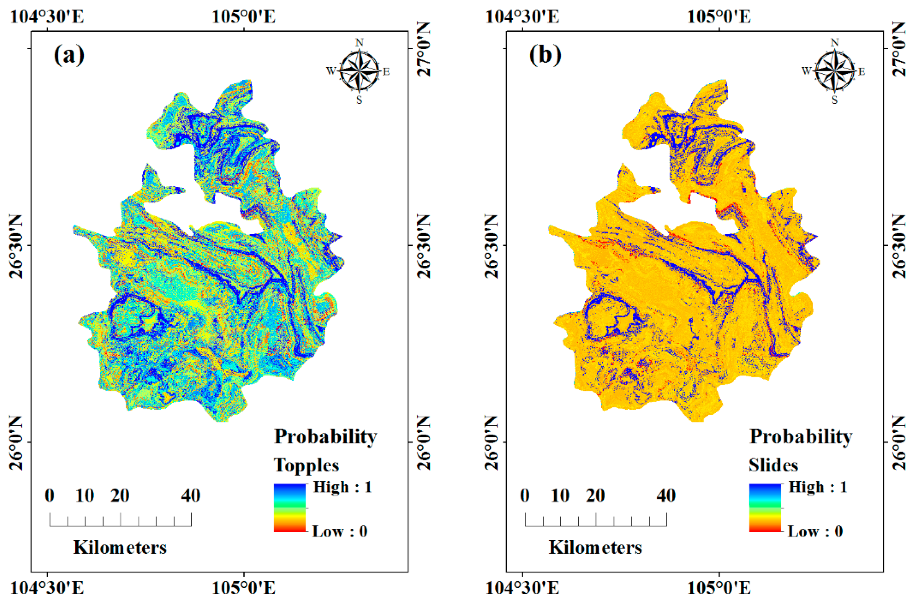
We have screened the factors of landslides through the GeoDetector model and used the BN model to train historical cases and predict the occurrence possibility and disaster loss level of landslides. Under the combination of various grades of factors based on the CPTs of each child node, each grid was assigned the results of three types of hazards. 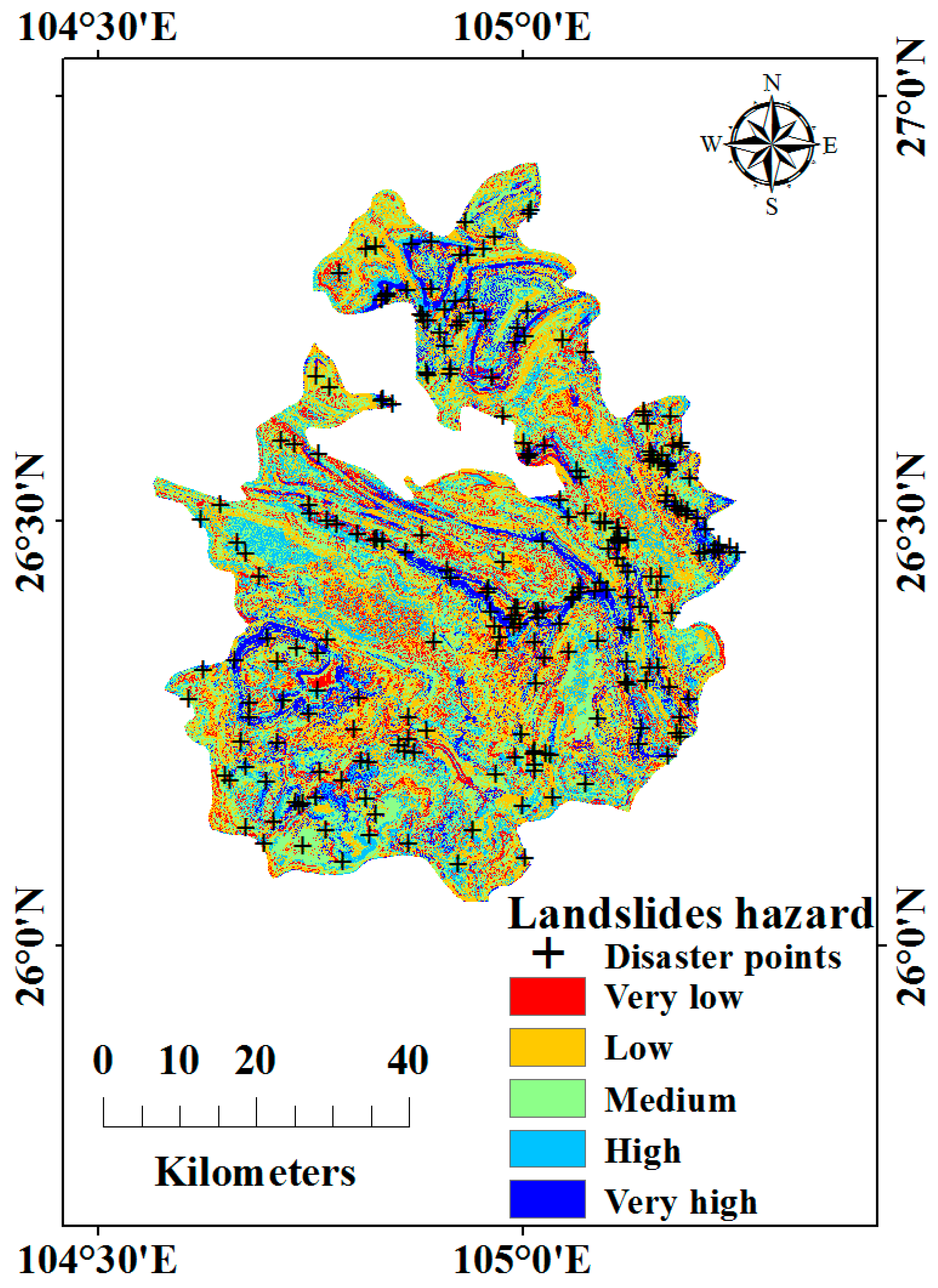The occurrence probability and disaster loss level of topples, slides, and debris flows spatial distribution maps were drawn by ArcGIS 10.6 (Figure 7). Then, the hazard index of each grid was calculated using a grid calculator tool based on Equation (5). For a better distinction, the hazard index values were reclassified into very low, low, medium, high, and very high using the Natural Breaks method. Finally, the construction of the LHM was completed (Figure 8).

To dualize the prediction results, we took the medium, high, and very high levels as the positive, low, and very low levels as negative and selected 72 disaster points in the verification set and random 72 non-disaster points to test the model.

Table 6. Model evaluation results using overall accuracy value (OA), Matthews correlation coefficient (MCC), and seed cell area index (SCAI).

Evaluation Methods	Test Data Set			Results
OA	Predicted		Actual	0.722
	Yes	No
MCC	54 (TP)	18 (FN)	Yes	0.445
	22 (FP)	50 (TN)	No
SCAI	Hazard levels	$P_{ai}$ (%)	$P_{di}$ (%)
	Very low	13.84	7.08	1.955
	Low	28.36	17.5	1.62
	Medium	30.56	22.92	1.333
	High	17.32	19.17	0.903
	Very high	9.92	33.33	0.298

lists the OA, MCC, and SCAI values of the model. The OA value is 0.722 and the MCC value is 0.445, both show that the model has high accuracy. The SCAI values reveal that the LHM is similarly accurate. In addition, $P_{ai}$ is the percentage of each class area in the total area, and $P_{di}$ is the percentage of landslide points in each risk level to total disaster points. The mean computed percentage risk level for the area is medium and more than 27% of the area is at high or very high risk, which means the entire study area has a higher potential for landslides risk. 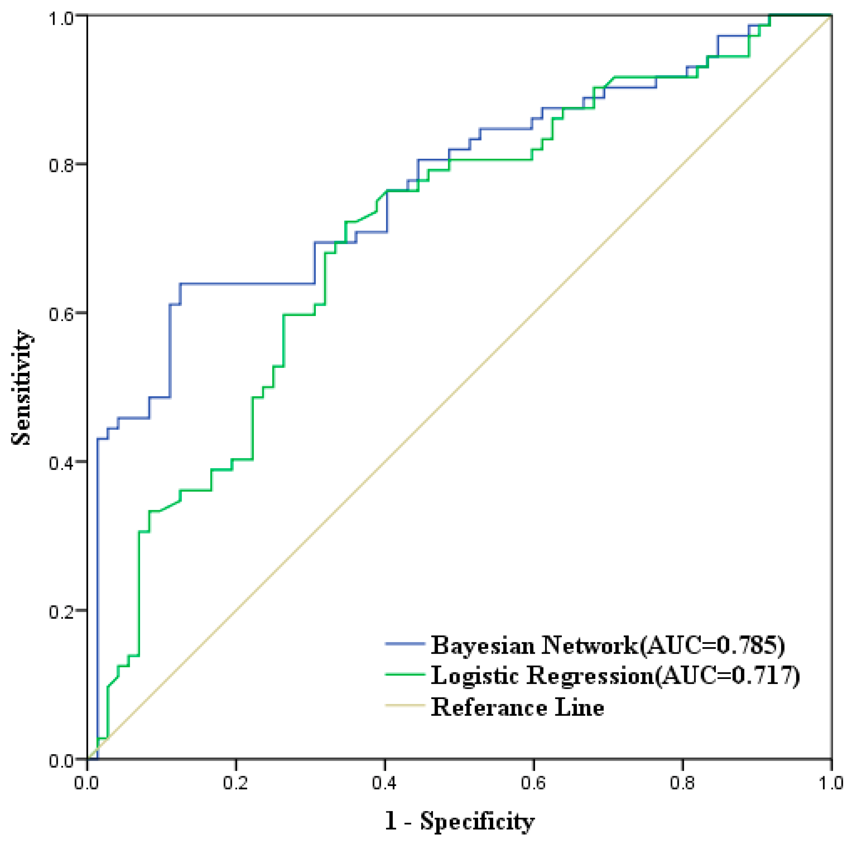Meanwhile, Figure 9 presents the ROC curves of the model using the test set. The AUC value is 0.785, meaning that the accuracy of the quantitative evaluation is 78.50%. In addition, we used the logistic regression model, which is a common simple method for landslide hazard assessment with an AUC value of 0.717; compared with the BN model we proposed, its AUC value is smaller, proving the reliability of the BN model (Figure 9). In addition, we referred to the satellite images which show that most of the historical landslides are located in the high-risk areas of LHM, proving the availability of the LHM framework.

5. Discussion

The formation of landslides is a very complex process, which is influenced by several topographic conditions and environmental factors, even anthropogenic ones, sometimes [65,66]. The construction of LHM is of great significance for the spatial differentiation analysis of landslide hazards. This work proposes the application of the GeoDetector and BN model for LHM in the case of Shuicheng County, China. We selected multi-source spatial data and condition factors to map the probability and risk level of topples, slides, and debris flows and finally constructed the LHM.

Removing redundant information is crucial to improve accuracy and calculate efficiency for LHM constructed by statistical theory methods. In this study, the redundant factors were eliminated using the GeoDetector model. We analyzed the explanatory power of each factor to the landslide hazard and the interaction between them. The results show that landslide hazard is greatly influenced by the topographic factors, mainly divided into elevation, slope, and geotechnical state factors such as lithology, geological age, and distance to faults. For extreme rainfall, the 50 mm daily rainfall is the closest threshold for inducing landslides in the study area. The result of the interactive driven analysis shows that some individual factors are not related to landslides alone but become more effective after interacting with other factors. This suggests that the interaction of different factors is more likely to trigger landslide and landslides are often caused by the combination of the whole factor system, which also proves the complexity of the landslides. Moreover, the GeoDetector model can effectively screen out influencing factors and be combined with various methods in different research fields.

Figure 7 shows the spatial distribution of topples, slides, and debris flows probability and risk level in the study area. It is obvious that the higher probability areas of topples, and slides are similar, but only a small part of them are the higher probability areas of debris flows. Because of the prerequisite condition with the rainfall–topples–slides–debris flows disaster chain mentioned above, only 40 of 195 slides points induce debris flows, which leads to the reversal of the higher vulnerability areas in the map of the debris flows probability. The spatial distributions of the risk levels of the three types of landslides are similar, and their high-level areas are mainly concentrated in fault zones and at high elevations. Figure 8 presents the final landslide hazard map based on the rainfall–topples–slides–debris flows disaster chain. The visual analysis of the LHM demonstrates that the higher hazard level areas are distributed as strip shapes, which are mainly affected by slope, elevation, and fault zones, with their geological age mainly concentrated in the Triassic and Permian Systems. Compared with the actual disaster points distribution, the higher-level areas contain most of the historical disaster points. The credibility of the model is also proved from the visualization.

In this paper, we established the confusion matrix and preliminary verification of each child node and evaluated the accuracy of LHM by OA, MCC, ROC curve, and SCAI. The results show that the landslide hazard assessment model we established has sufficient accuracy. In addition, the statistical results of the SCAI also show that more than 77% of the historical hazard sites in the study area occurred in areas of medium to high risk, which also demonstrates the availability of the model in reality. Compared with the researches of LSM constructed by other machine learning methods, they use binary classification for a single type hazard, and do not consider the whole system of landslides. BN model can construct a complex causal network and calculate the probability and risk level of multiple disasters simultaneously.

In contrast to previous studies [21], We not only discuss the “Single factor driven analysis” but also list the “Factors interaction driven analysis” in the GeoDetector model on landslide hazards, which is the first time in LSM research. In addition, we select different levels of rainfall factors and use factor screening to determine the rainfall thresholds that are most likely to induce landslides. In using the Bayesian network model, we greatly increased the resolution [67], and extended the LSM study to LHM based on risk level, and selected the rainfall–landslides disaster chain as the study object. Moreover, we used multiple validation methods to evaluate the accuracy of the framework we proposed.

In this study, the LHM was drawn by analyzing three types of landslides according to a rainfall–landslide disaster chain and combining the quinary classification risk level of each disaster. Compared with LSM by various methods, the causality network of LHM is more complicated, the calculation method is more difficult, and the classification factors need to be considered more. Therefore, this paper makes use of the advantages of the BN model to calculate such a complex disaster chain process on the premise of higher accuracy. It is also widely available and repeatable. Moreover, we greatly improved the grid pixel size (30 × 30 m) and screened factors by the GeoDetector model using 16 factors from different angles. All the above are the key points of this study and the advantages of this framework. Our results indicate that the research framework based on the GeoDetector model and the BN model is a promising and robust technique for LHM.

6. Conclusions

Landslides are among the most frequent natural hazards. Topples, slides, and debris flows are the three most important types of landslides. Based on the rainfall–topples–slides–debris flows disaster chain, this study established a framework for LHM in Shuicheng County, China. This framework consists of the GeoDetector and BN models, where the GeoDetector model was used to screen 16 factors from multi-source data, eliminate redundant information, and discuss the interaction between factors, while the BN model was used for constructing a causality network within the disaster chain and determining the probability and risk level of the three types of landslides. The framework performs well and can be extended to other areas, including other research fields. The evaluation of this work was conducted using OA, MCC, ROC curve, and SCAI. The following can be inferred from the results of this study. First, landslide hazards are mainly affected by geographical factors and geotechnical conditions, and 50 mm daily rainfall is the most likely threshold to induce hazards in our study area. Second, this framework is effective and convenient for LHM. Finally, the evaluation results show that this framework is sufficiently accurate to construct complex LHM. In summary, the combination of the GeoDetector and BN model is very promising for the hazard assessment of landslides. We will collect more multi-source data and seek more advanced methods to improve the accuracy of LHM in the future.