Assessing the Groundwater Quality in the Liwa Area, the United Arab Emirates

Abstract

Last period groundwater quality raises big concerns all over the world since it is a limited source of drinkable water and for agricultural and industrial use. While the suitability of the groundwater of Liwa aquifer (Abu Dhabi Emirate) for agricultural use has been previously partially studied, not all the water parameters have been taken into account. Therefore, in this paper, we propose the study of 42 concentrations series of 19 groundwater parameters. We test the hypothesis that the water parameters series recorded at different locations are similar and group the samples in clusters. The main parameters that determine the differences between the clusters are determined by Principal Component Analysis (PCA). Finally, we use a quality index for assessing the water suitability for drinking. The conclusions emphasize the necessity of using more than one technique to evaluate water quality for different purposes and to cross-validate the results.

1. Introduction

All over the world, billions of people suffer from water scarcity because less than 1% of the world’s water is fresh and accessible [1]. The remediation of polluted aquifers is generally difficult and in many cases, is not possible. Therefore, the study of water quality is an essential study topic for water resources scientists [2,3,4,5,6,7,8,9,10,11,12] as a first step for taking informed measures for keeping it clean and as a warning for reducing its pollution [12].

MIKE-II, QUASAR, QUAL2E, and CE-QUALW2, SIMCAT, TOMCAT are water quality models providing comprehensive modeling of water quality conditions in river systems [13]. They are developed for particular purposes and none of them are best. For assessing the surface water quality, researchers [14,15,16,17,18,19] introduced water quality indices (WQI), the most known being CCMEWQI [16]. A review of the most important ones, containing their composition, structure, and comparison is provided in [14]. Other approaches use univariate statistical methods, as time series analysis, for describing the temporal [6,7,8,10] evolution of some water parameters. Bhat et al. [8] and Ioele et al. [20] employed multivariate statistical tools. ANOVA is utilized for evaluating the differences among the series of water quality variables recorded at the study sites. Cluster analysis (CA) allows selecting the groups of sites with similar characteristics (concentrations, pH) of water parameters. Principal Component Analysis (PCA) leads to the detection of the main water parameters that influence water quality [20]. Gad et al. [21] combined a drinking water quality index and four pollution indices, principal component analysis (PCA), partial least squares regression (PLSR), and stepwise multiple linear regression (SMLR) to evaluate the water quality for drinking purposes in the Nile Delta.

Assessing the groundwater quality became a study topic in 1968 when the ‘‘groundwater vulnerability’’ notion was introduced by Margat [22]. The definitions of this concept [22,23,24] aim at catching the interaction between a contaminant applied in the soil vicinity (or its surface) and the aquifer, during the pollutant’s transportation by the rainwater. The physicochemical reactions and their effects on the groundwater depend on hydrogeological conditions and the pollutant characteristics, quantity, and exposure time [25,26,27].

The study of groundwater quality and the risk to pollutants’ exposure is generally done by using the DRASTIC model, introduced by Aller et al. [28], DRASTIC-like methods (AVI [29], DIVERSITY [30], GOD [31], ISIS [32], PRAST [33], SINTACS [34,35,36], etc.), and their versions (DRAMIC [37], DRIST [38], DRAV [39], DRASTIC-LU [40], DRASIC-LU [41], SINTACS-LU [42,43], DRASTICA [44,45], etc.). For a review of these methods, the reader may refer to [46]. Specific methods for studying the karst aquifer vulnerability are also employed; among them are COP [47], EPIK [48], REKS [49], RISKE [50,51], PaPRIKa [52], and PI [53]. GIS is an important tool in these cases for drawing the vulnerability maps [54,55].

For assessing the groundwater suitability for drinking or agricultural use at different locations, scientists [56,57,58,59] use indices like Chloro-alkaline index (CAI), Saturation index (SI), Sodium Absorption Ratio (SAR), Residual Sodium Carbonate (RSC), Kelley’s ratio, and magnesium hazard. A single WQI (single-factor pollution index (I), the nemerow pollution index (NI), heavy metal evaluation index (HEI), the degree of contamination (Cd)), or geostatistical methods can also be utilized to emphasize the groundwater pollution at a regional scale [60,61].

In this article, we propose a combined methodology for studying the groundwater characteristics at a regional scale. Firstly, we test the similarity of the series of water parameters (collected at different sites), then we cluster the sites with the same characteristics and perform the Principal Components Analysis (PCA) for extracting the significant components. Then, we assess the suitability of water for drinking using a water quality index. Finally, we compare the obtained results with those provided by the literature and conclude.

2. Study Area and Methods

2.1. Study Area

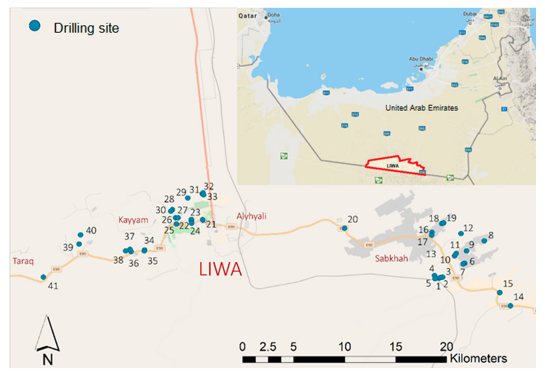
Abu Dhabi Emirate, the largest emirate of the United Arab Emirates, is situated along the Arabian Gulf, between 22.5° and 25° north latitudes and 51°–55° east longitudes. The study area, Liwa, belongs to Abu Dhabi Emirate. Water samples were collected in the northern part of the Liwa Crescent, between Madinat Zayed and Meziyrah. The distribution of the drilling wells is presented in Figure 1, whereas their coordinates are given in

Table 1. Coordinates of the drilling locations.

Sample No.	Coordinates		Sample No.	Coordinates		Sample No.	Coordinates
	North	East		North	East		North	East
1	23.05.07	53.59.44	15	23.04.21	54.02.56	29	23.09.21	53.46.27
2	23.05.09	53.59.49	16	23.07.32	53.59.21	30	23.08.39	53.45.33
3	23.05.10	53.59.55	17	23.07.23	53.59.20	31	23.09.34	53.47.13
4	23.05.15	53.59.29	18	23.08.00	53.59.52	32	23.09.37	53.47.15
5	23.05.05	53.59.31	19	23.08.02	53.59.58	33	23.09.31	53.47.17
6	23.05.54	54.01.05	20	23.07.45	53.54.44	34	23.06.36	53.44.10
7	23.05.52	54.01.00	21	23.08.12	53.47.14	35	23.06.33	53.44.09
8	23.07.05	54.02.07	22	23.08.08	53.46.38	36	23.06.31	53.43.27
9	23.06.33	54.01.11	23	23.08.13	53.46.38	37	23.06.38	53.43.24
10	23.06.18	54.00.33	24	23.08.01	53.46.39	38	23.06.33	53.43.10
11	23.06.25	54.00.38	25	23.07.58	53.45.51	39	23.06.55	53.40.42
12	23.07.28	54.00.53	26	23.08.18	53.45.48	40	23.07.24	53.40.47
13	23.06.39	54.59.45	27	23.08.18	53.45.56	41	23.05.10	53.38.49
14	23.03.39	54.03.30	28	23.08.44	53.45.38

.

The mean monthly temperature in the region is between 20 °C and 35 °C, with minima between 13 °C and 29 °C and maxima in the interval 31 °C–48 °C. The average humidity varies from 59% to 68%, with a maximum of about 79%. The maximum monthly average precipitation recorded from 2003 till 2017 was 16 mm (in December) and 10 mm (in January), without precipitation from May to October.

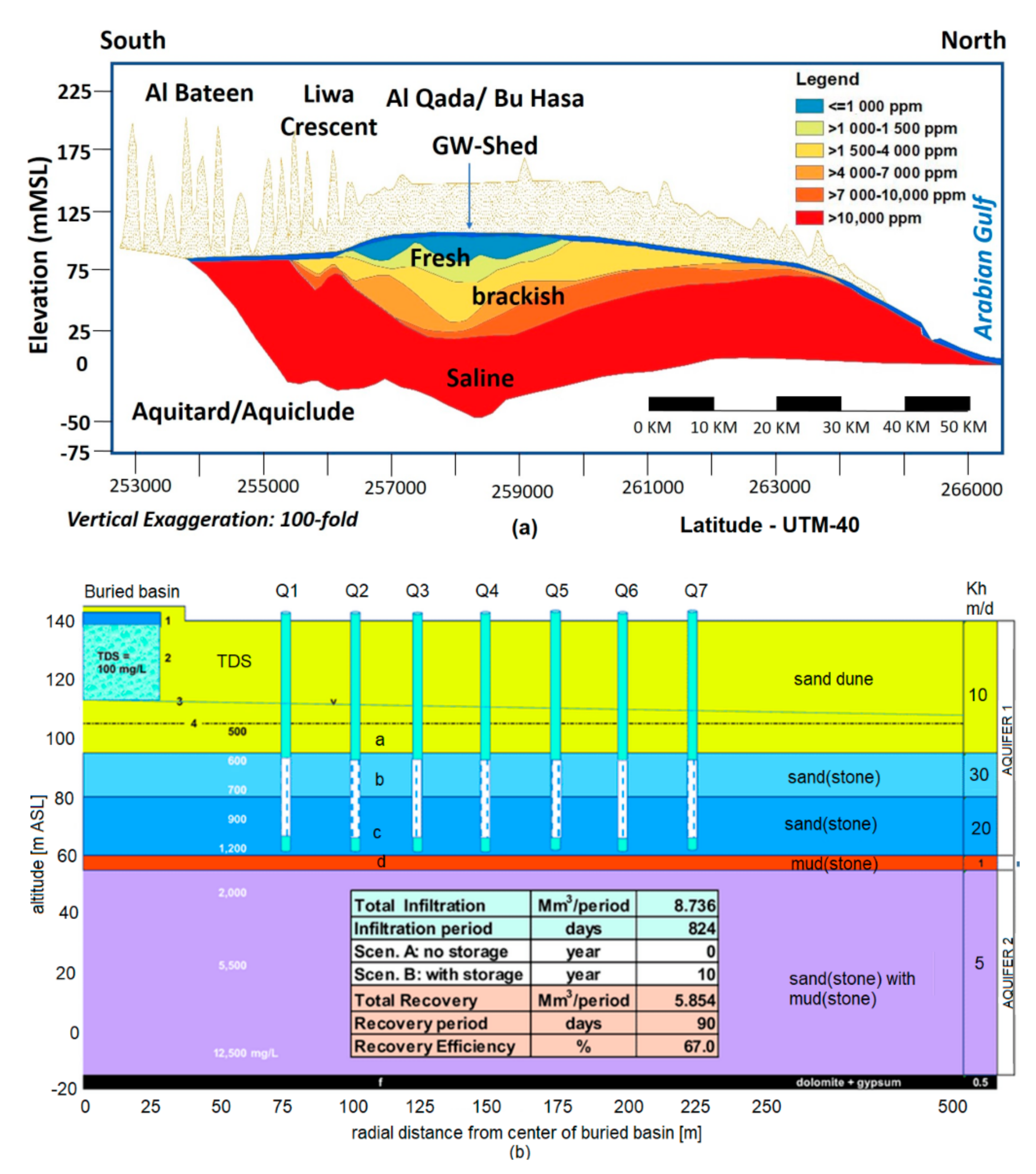
In the Liwa area, continental and shallow water marine sedimentary rocks were deposited from Cambrian to Quaternary. Liwa’s aquifer lithology is composed of two essential stratigraphic units. The first one has a thickness between 100 m and 150 m and is formed by a Quaternary part, Holocene, and Pleistocene Aeolian fine to medium sands and interdunal deposits. The second one, with a thickness of over 350 m, is a Tertiary unit formed by mudstones, evaporites, and clastics of Miocene age [62]. The shallow aquifer formation consists of sand and sandstone, with a variable thickness underlain by siltstone, claystone, and evaporites. In the Liwa area, the altitude of the groundwater level is between 60 m and 107 m a.s.m.l. (above mean sea level). The shape of the groundwater table is concave down, elongated from East to West. Its top is situated approximately 25 km north of Mezairaa [63]. The gradient of the groundwater table is less than 0.5 m/km in the east-west direction, 0.5 m/km in the southern part, and more than 1 m/km in the northern region.

The principal aquifer of the Western Region, situated in the northern Liwa area, consists of the upper subunit of the Quaternary sediments. To the west, the aquifer extends to the Sabkha Matti area, while to the East, it borders the gravel plains located at the foot of the Oman Mountains. The average thickness of the principal aquifer varies between 30 m to 50 m. Overlaying sands dunes, forming a thick unsaturated zone, cover the aquifer. The lower subunit of the Quaternary sediments represents a fully saturated aquitard, situated above the aquiclude consisting of the Tertiary Lower Fars unit [62,63] area, while to the East, it borders the gravel plains located at the foot of the Oman Mountains. The average thickness of the principal aquifer varies between 30 m to 50 m. Overlaying sands dunes, forming a thick unsaturated zone, cover the aquifer. The lower subunit of the Quaternary sediments represents a fully saturated aquitard, situated above the aquiclude consisting of the Tertiary Lower Fars unit [62,63]. A schematic description of the Liwa aquifer and well cross-section are shown in Figure 2.

2.2. Experimental Study

For the present study, we collected groundwater samples from 41 wells situated in the Liwa zone in March 2018 and stored them in polyethylene bottles of 1 L capacity. We followed the methods of the American Public Health Association for the samples’ preservation and analysis [64].

pH, electrical conductivity (EC), and total dissolved solids (TDS) were determined at the sampling sites using a pH-meter, a portable EC-meter, and a TDS-meter (Hanna Instruments, Ann Arbor, MI, USA). The sodium (Na⁺), potassium (K⁺), magnesium (Mg²⁺), and calcium (Ca²⁺) ions were determined by atomic absorption spectrophotometry (AAS), while the carbonate and bicarbonate were analyzed by volumetric methods. Sulfate (SO₄²⁻) was estimated by the colorimetric and turbidimetric methods. The nitrate concentration was measured by ionic chromatography. Trace elements (Cd, Cr, Zn, Pb, Cu, Ni, Mn) were determined by Inductively Coupled Plasma spectrophotometer (ICP-OES, Agilent, CA, USA). One can find the results of the chemical analyses in [62].

2.3. Methodology

The statistical analysis performed on the series of water parameters consisted of the following.

⮚

Determine the variability of the water parameters at different locations

For this aim, the basic statistics, the histograms, and the boxplots of the series were studied. Comparisons of the series values with the maximum admissible limits have also been performed.

⮚

Study of the similarity of the series collected at different sites

For the rest of the study, except for the computation of the water quality index, data were standardized by dividing the concentration of each element by the maximum concentration of the element. Then, to test the hypothesis that there is no statistically significant difference between the water elements in the samples collected at different study places, the Kruskal-Wallis nonparametric test [65] was performed at a 5% significance level. If the null hypothesis was rejected, the Dunn post hoc test was applied to determine the pairs of dissimilar samples [66].

⮚

Perform data clustering

The classification of the series into homogenous groups within which the patterns are the same was done by using the k-means clustering algorithm [67]. This algorithm determines groups of data series based on a criterion of error minimization, which computes the distance of instances to their representative values. The stages of the k-means algorithm are summarized below [68,69,70].

Let us consider that $Z=(z_1,z_2,\dots ,z_m),z_i\in {\mathbf{R}}^n,i=\overline{1,m}$, is the vector that contains the series concentrations measures at each location (column j is composed of data from site j).

(1)

Firstly, the number of clusters, k, is selected.

This number is either introduced by the user or computed based on different algorithms. Among the methods used to determine the optimal number of clusters, the most popular are the elbow, the silhouette, and the gap statistic methods [71]. In this article, we employed the facilities of the R software, especially the NbClust, which provides 30 algorithms for the detection of the optimal k. The best number of clusters is selected according to the majority rule [72].

(2)

The clusters’ centroids ${\vartheta }_1,\dots ,{\vartheta }_k\in {\mathbf{R}}^n$ are initialized and the distances between the data points and the cluster centers are computed. Each point is assigned to the cluster that minimizes the distances from it to the clusters’ centers.

(3)

The new clusters’ centers are determined, the procedure restarts from (2) and runs until no data point can be reassigned to another cluster. Then, stop.

⮚

Perform the Principal Component Analysis (PCA) [73,74,75]

In hydrological studies, PCA is a tool for finding the water quality parameters that describe the processes that govern the groundwater chemistry and extract valuable information using only the significant variables. PCA is a statistical procedure of the multivariate analysis, designed for reducing the variables’ number and replacing them with a few artificial ones (Principal Components—PCs). These PCs are independent factors that mainly explain the study phenomenon and sum up a significant amount of variance. There are many criteria used for extracting the principal components; among them, the most used are the Catell Scree plot, the Kaiser criterion (Kaiser), and the Explained Variance Criterion. The first PC accounts for the highest variability are emphasized on the Scree plot [74]. Kaiser criterion [76] takes into account the selection of those PCs that correspond to eigenvalues greater than 1 [77]. Here, we used both the Scree plot and the Kaiser criteria for detecting the PC.

The biplot shows the contributions of the variables on the PCs. The loadings emphasize the correlations between the input variables and the factors.

For a deeper insight into the PCA and its implementation in R software, the reader may see [74,75,78,79].

⮚

Assessing the suitability of water for drinking

For this aim, we used a weighted arithmetic Water Quality Index (WQI) [80,81,82]. The WQI index is built as follows:

(1)

choose the water parameters used in the computation;

(2)

compute the quality rating (q_i) for each parameter by:

$$q_i=\frac{C_i-C_{ideal}}{S_i-C_{ideal}},$$

(1)

where C_i is the actual concentration in sample i, $1/S_i$ is the admissible value, and $C_{ideal}=0$ for all, but pH, for which $C_{ideal}=7$;

(3)

Compute the weight of each water parameter, i, by:

$$w_i=\frac{1/S_i}{{{\displaystyle \sum }}_{i=1}^n(1/S_i)},$$

(2)

where n is the number of water parameters taken into consideration;

(4)

Compute the WQI by:

$$WQI={{\displaystyle \sum }}_{i=1}^n(w_i Q_i),$$

(3)

(5)

Classify the water quality based on the interval in which the value is contained. The classes and the corresponding intervals are A (Excellent)—(0,25], B (Good)—(25,50], C (Poor)—(50,75], D (Very poor)—(76,100], and E (unsuitable) > 1000 [80].

(6)

Compare the values of WQI for the samples contained in different clusters.

3. Results and Discussion

Table 2. Basic statistics of the water parameters.

	Minimum	Maximum	Average	Standard Deviation	Variation Coefficient (cv)
pH	6.1900	7.190	6.519	0.256	0.039
EC (μS/cm)	328.0000	3003.000	1478.488	648.574	0.439
TDS (mg/L)	136.0000	1565.000	863.049	354.590	0.411
Na+ (mg/L)	638.1750	5302.039	2923.174	1044.109	0.357
K+ (mg/L)	2.7043	17.203	8.964	3.121	0.348
Cl− (mg/L)	827.0140	9628.939	5670.833	2258.713	0.398
NO3− (mg/L)	0.4259	2.486	1.410	0.550	0.390
SO42− (mg/L)	4.1290	45.794	23.570	9.142	0.388
CO32− (mg/L)	14.4000	108.000	57.712	27.473	0.476
HCO3− (mg/L)	14.6400	236.680	87.546	48.842	0.558
Ca2+ (mg/L)	104.2060	1244.785	705.423	269.035	0.381
Mg2+ (mg/L)	21.5390	672.509	316.744	148.690	0.469
Cd (mg/L)	0.0001	0.002	0.001	0.000	0.762
Cr (mg/L)	0.0005	0.023	0.015	0.005	0.362
Cu (mg/L)	0.0009	0.004	0.002	0.001	0.433
Mn (mg/L)	0.0001	0.011	0.002	0.003	1.242
Ni (mg/L)	0.0005	0.004	0.002	0.001	0.563
Pb (mg/L)	0.0013	0.012	0.005	0.003	0.500
Zn (mg/L)	0.0004	0.052	0.005	0.010	2.135

contains the basic statistics of the study data series.

High amplitudes of the registered values are found for almost all study elements, with very high standard deviations for EC, TDS, Na⁺, Cl⁻, Ca²⁺, and Mg²⁺. The higher the standard deviation is, the higher the variation of the values of a series about the mean is. The coefficients of variation show high variability of Zn, Mn, Cd, and Ni concentrations by comparison to the other series.

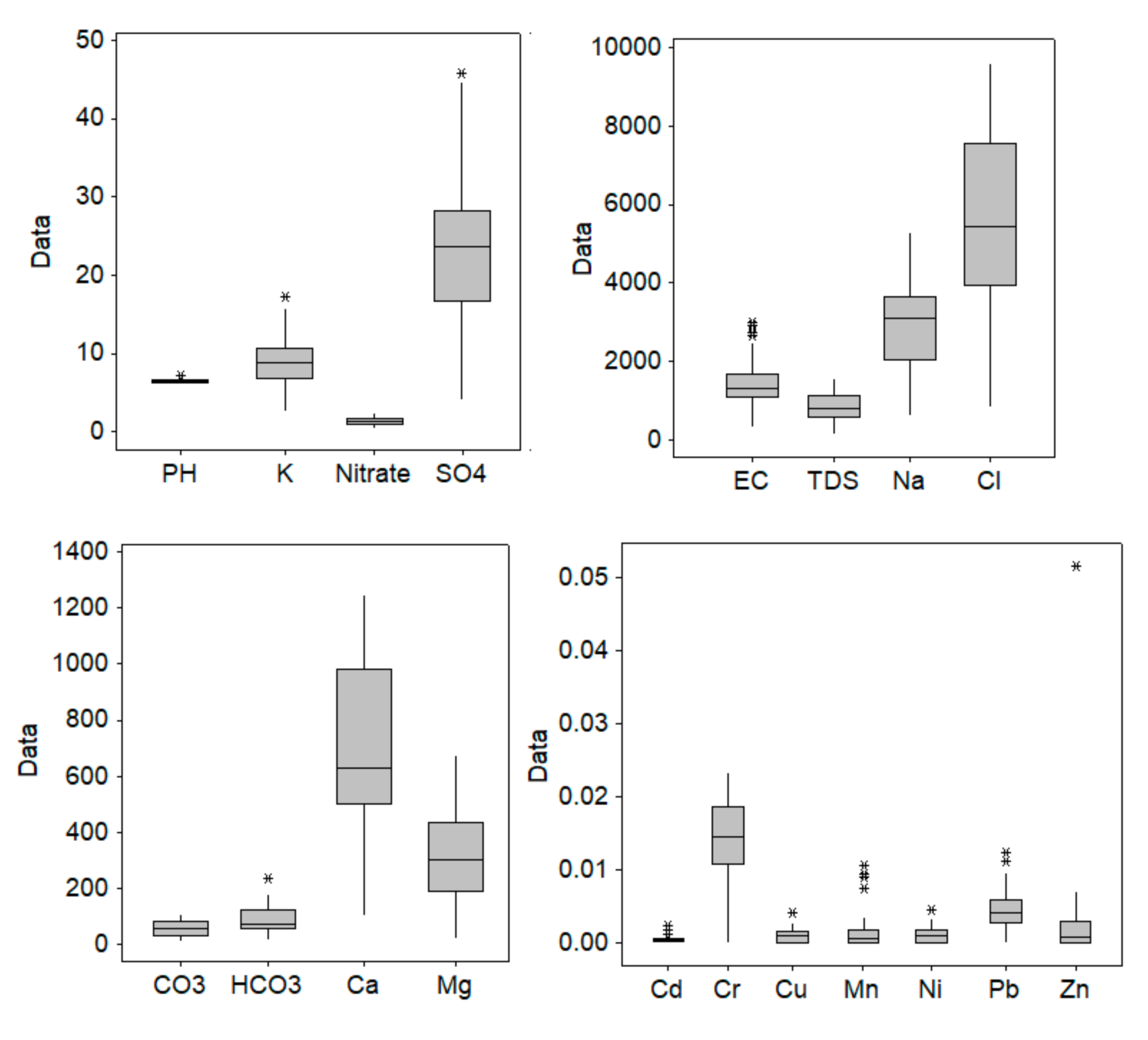
The boxplots of data series (Figure 3) show the existence of some outliers for pH, K⁺, SO₄²⁻, EC, HCO₃⁻, Cd, Cu, Mn, Ni, Pb, and Zn series.

In the presence of outliers, the standard deviation becomes high. This is the situation, for example, for the EC series, which presents very high outliers (3003, 2995 μs/cm) compared to the other values, significantly augmenting the standard deviation.

Still, the pH remains in the admissible limits, its values being between 6.19 and 7.19. Also, the groundwater is not contaminated with Cd, Cr, Cu, Mn, Ni, and Zn, with the maximum concentrations of these elements being well below the admissible limits (0.003, 0.05, 2, 0.5, 0.07, and 3 mg/L, respectively). Only samples 9 and 11 contain Pb in concentrations (0.1117 and 0.01229 mg/L) greater than the prescribed limit (0.01 mg/L).

Comparing the determined values of the water parameters with the WHO’s drinking water standards [57,83], it results that Na⁺ and chlorides concentrations exceeded the admissible potability limits (200 mg/L and 250 mg/L, respectively) between 3.19 and 26.51 times (for Na⁺) and between 4.13 and 48.14 times (for chlorides), respectively. In the aquifer system, sodium is mainly derived from the dissolution of salt minerals and silicate weathering [84]. EC has 80% of values above the permissible limit for drinkable water (1000 μs/cm). The variation of EC values could be explained by rock water interaction and anthropogenic influences, like agricultural run-off and wastewater discharges [57]. TDS has 80.5% of values above 600 mg/L, with 35.7% of water samples being in the category of highly undrinkable water (>1000 mg/L).

The concentrations of Ca²⁺ exceed the permissible limits (75 mg/L) between 1.39 and 16.60 times. The contribution of Ca²⁺ content in water is dependent on the solubility of CaCO₃ and CaSO₄ [85].

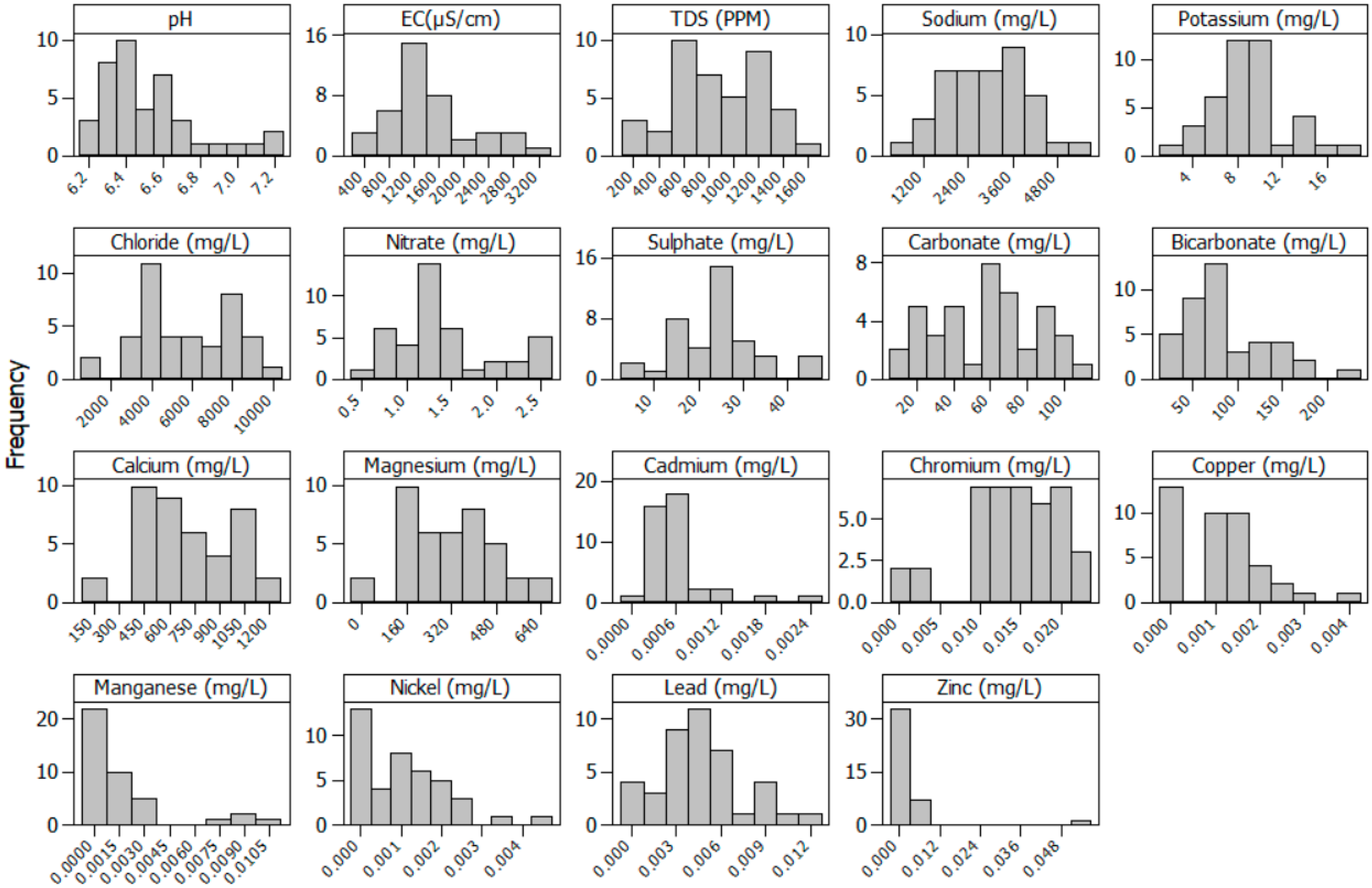
Figure 4 presents the histograms, showing asymmetric and non-uniform distributions of the water parameters. Zn, Cd, Mn, and Co series present the highest right—skewness, whereas Na⁺ and K⁺ have the lowest asymmetry.

The Kruskal-Wallis test rejected the null hypothesis that the data series obtained at different sites have the same distribution. The post hoc Dunn test emphasized the dissimilarities between the samples, listed in

Table 3. Diagonal table of dissimilarities that resulted from the Dunn test.

1; 21, 26, 27, 41	15; 21, 26, 27, 40, 41	29; -
2; 7, 9, 11	16; 21, 26, 27, 40, 41	30; 34
3; 7, 9, 11, 26	17; 21, 26, 27, 40, 41	31; -
4; 26, 27	18; 34, 35	32; 34
5; 18, 19, 21, 23, 25–27, 29, 30, 32, 33, 40, 41	19; 34	33; 34, 35
6; 12, 18, 19, 21–33, 40, 41	20; 21, 26, 27	34; 40, 41
7; 12, 18–33, 37, 38, 39, 40, 41	21; 34–37,39	35; 40, 41
8; 18, 21, 26, 27, 30, 32, 33, 40, 41	22; -	36; -
9; 12, 18, 19, 21–33, 40, 41	23; 34	37; -
10; 18, 21, 23, 25–27, 30, 32, 33, 40, 41	24; -	38; -
11; 12, 18, 19, 21–33, 40, 41	25; 34	39; -
12; -	26; 34–39	40; -
13; 21, 26, 27, 30, 32, 33, 40, 41	27; 34–37, 39	41; -
14; 18, 19, 21, 23, 25–27, 30, 32, 33, 40, 41	28; -

. The significance of the numbers’ combinations is explained in the following. For example, in the first column and the fourth row, “4; 26, 27” means that Sample 4 and Sample 26 do not have the same distribution and Sample 4 and Sample 27 also do not have the same distribution. On another hand, in the first column and 12th row, “12; -” means that there is no dissimilarity between Sample 12 and all the samples with a label greater than 12. Being a diagonal table, the dissimilarities with the samples labelled with a number smaller than 12 are already displayed in the previous rows (and first column); in this example, these are 6, 7, 9, and 11.

One can also see that samples 40 and 41 are not similar to samples 5–11, 13–17, 34, 35; samples 18, 19, 21, 23, 25–27, 30, 32, 33 are not similar to 5 and 6; and samples 12, 18, 19, 21–33 are not similar to 7 and 9, and so on. These dissimilarities are originated in the concentrations of some groundwater elements.

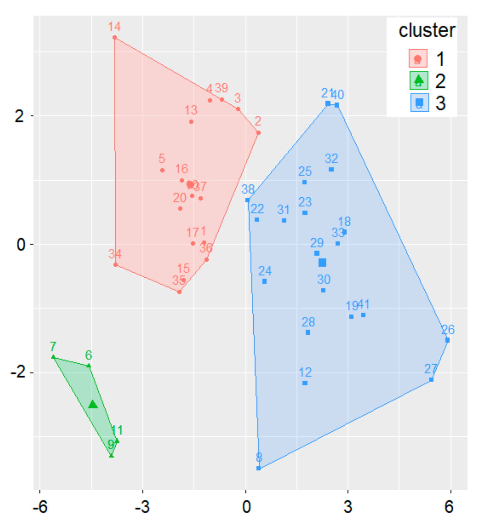
To classify the water samples based on their chemical composition, clustering has been performed. The best number of clusters was found to be 3. The clusters are presented in Figure 5.

There is a clear separation between the clusters, as expected for a good clustering.

Comparing the results from

Table 4. Principal Component Analysis (PCA) Summary—the first nine principal components (PCs).

	PC1	PC2	PC3	PC4	PC5	PC6	PC7	PC8	PC9
Standard deviation	2.6936	1.6215	1.2924	1.1733	1.0402	0.9941	0.9708	0.8309	0.7715
Proportion of variance	0.3819	0.1384	0.0879	0.0725	0.0569	0.0520	0.0496	0.0363	0.0313
Cumulative proportion	0.3819	0.5203	0.6082	0.6806	0.7376	0.7896	0.8392	0.8755	0.9068

and Figure 5, one can remark their concordance. For example, 6, 7, 9, and 11 (situated in the second cluster) are not in the same cluster as 12, 18, 40, and 41 (situated in the third cluster); 15, 16, and 17 (situated in the first cluster) are not in the same cluster as 21, 26, 27, 40, and 41 (situated in the third cluster).

The sites in the first cluster are mainly situated along communication roads, so the effect of pollution is higher. The water in this cluster is highly undrinkable: TDS >1000 ppm, the sodium content is at least 12 times bigger than the admissible value (200 mg/L), the chloride content is more than 20 times higher than the upper limit (250 mg/L).

For the elements in the second cluster, pH is between 6.12–6.92, EC in the interval 2465–3003 (µS/cm), and TDS is between 1287 and 1585 ppm (higher than the values determined in the samples from the first cluster). The sodium and potassium concentrations in the samples from the second cluster are generally higher than those in the samples from the first one: the average values in the second (first) cluster are 3870 (3733) mg/L and 13.24 (10.74) mg/L, respectively. The same is true for the chlorides for which an average of 8630 (7277) mg/L is detected in the second (first) cluster.

Significant differences are found between the average values of carbonate, bicarbonate calcium, and magnesium, which are 87.6, 32.94, 1125, and 587 mg/L for the second cluster, whereas for the first one, they are 50.18, 106.59, 856, and 349 mg/L, respectively.

The mean concentrations of Cu and Zn (Pb) are 3 and 2.5 times higher (4 times smaller), respectively, in the second cluster by comparison to the first one.

The third cluster is characterized by the lowest TDS (603.35 pm), Na⁺ (2045 mg/L), K⁺ (6.7 mg/L), Cl⁻ (3714 mg/L), CO₃²⁻ (58.13 mg/L), and Ca²⁺ (494 mg/L) concentrations. The average concentrations of lead and zinc are about 1.7 times higher than those from the first cluster. Comparable concentrations of Mn are recorded in the second and third clusters, whereas concentrations of Cu are about 1.4 bigger in the second cluster than in the third one. The nitrates, sulfates, and Ni concentrations are the highest in the samples from the second cluster and the lowest in the last one.

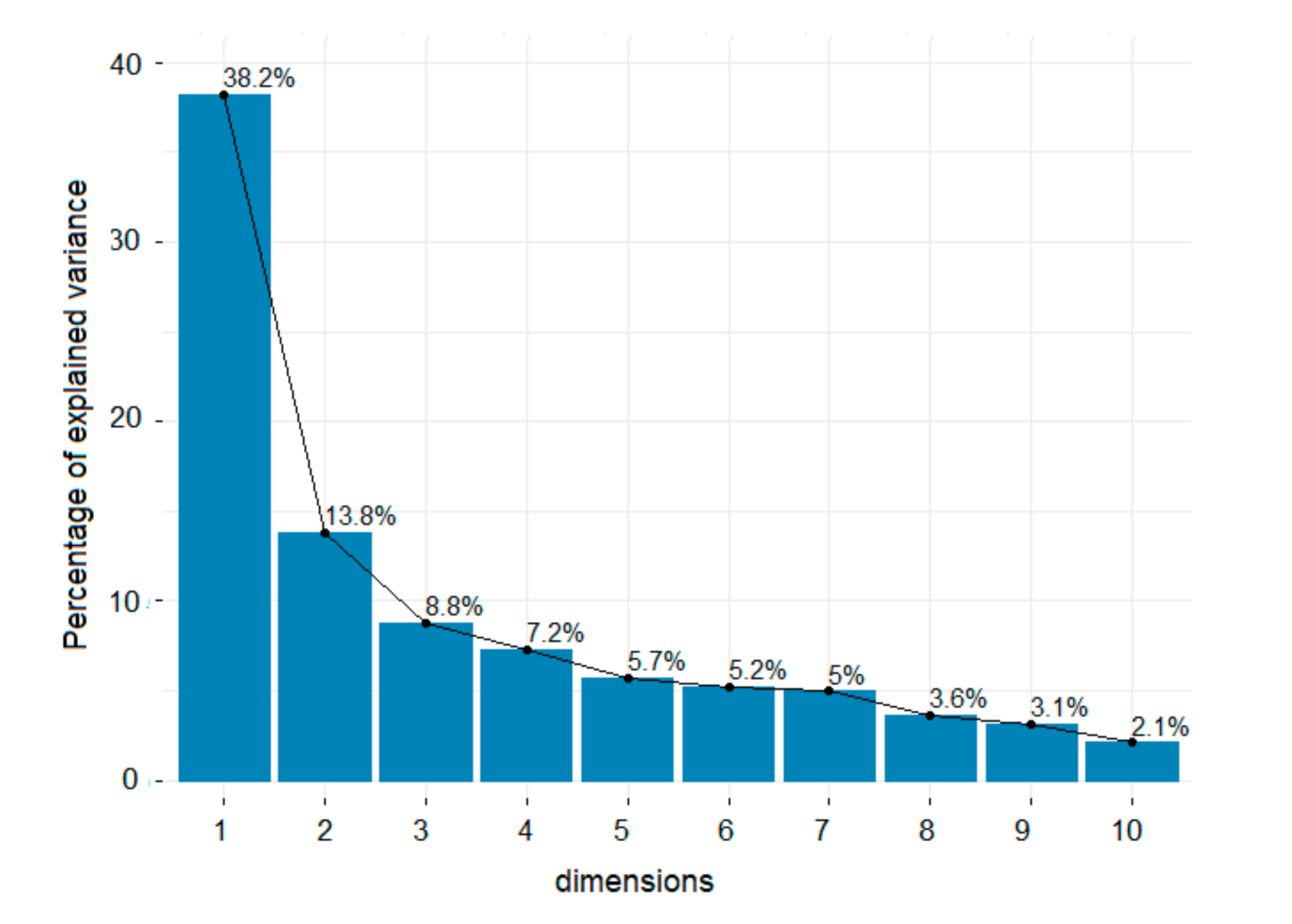
The next step was to perform PCA for selecting the main components that determine the water quality. The Scree plot (Figure 6) was used for selecting the principal components (PCs). Figure 6 shows that the first two components have the highest contribution to explain the variance (38.2% and 13.8%).

Table 4 shows the summary of PCA (standard deviation, the proportion of variance, and cumulative proportion) for the first eight PCs. Generally, the selected principal components are those of which their corresponding eigenvalues are greater than 1. In this case, the first five components have eigenvalues greater than one and explain 73.76% of the variance (which is an acceptable percentage). Since the percentage of explained variation is high, we shall keep only PC1–PC5.

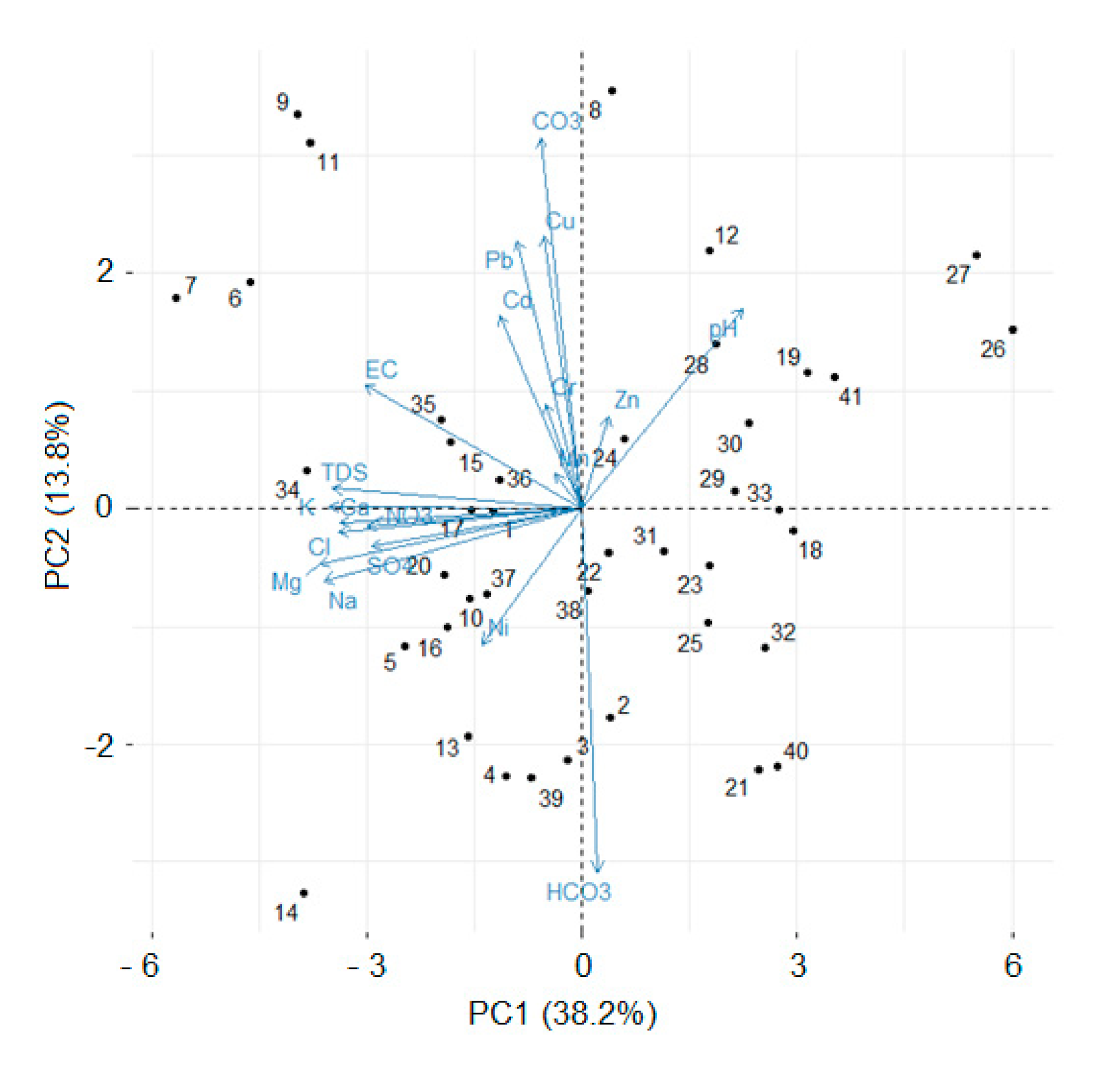
The contributions of the variables on the first two PCs are presented in the biplot (Figure 7).

The distances from the variables to the origin represent the variables’ quality on the factor map. The pairs (pH and Ni), (CO₃²⁻, and HCO₃⁻) are strongly negatively correlated (since the segments represented in Figure 7 are opposite). Sites 7, 6, 9, and 11 (Figure 7, top left-hand side) are opposite to 26 and 27 (Figure 7, top right-hand side), reconfirming the classification of the four sites (7, 6, 9, and 11) in a separate cluster. The same is true for sites 7, 6, 9, and 11 on one hand and 14 on the other one.

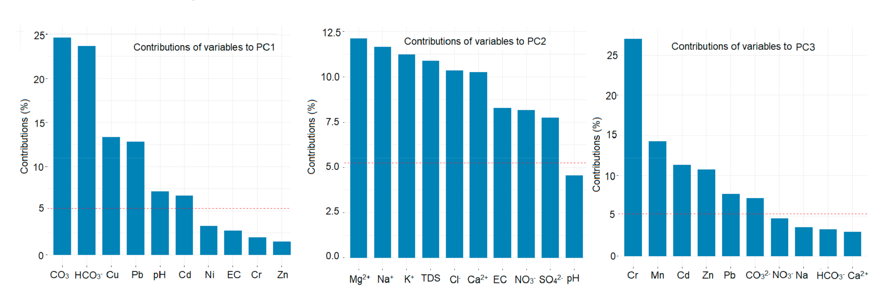
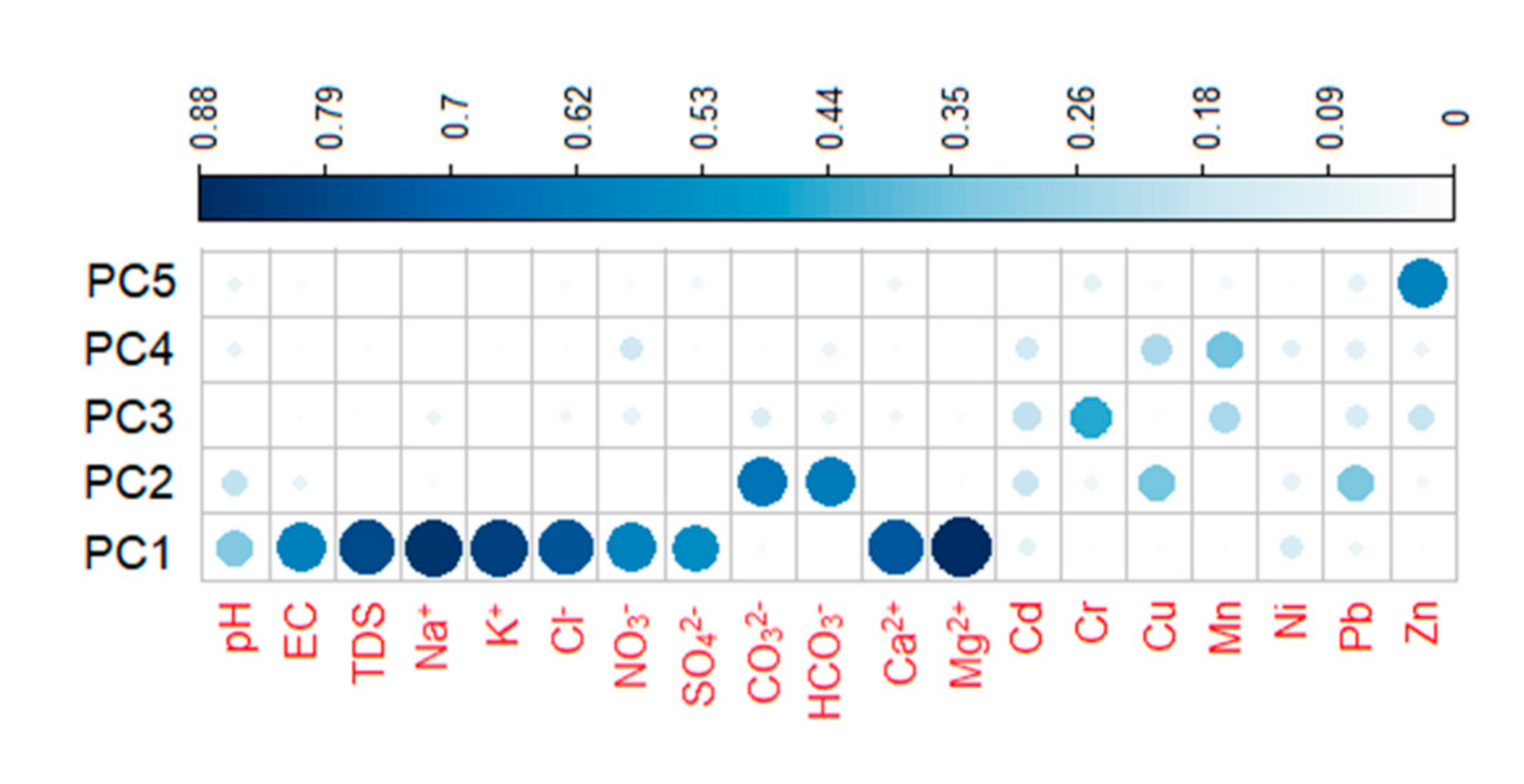
The variables whose distances to the origin are high are well represented on the factor map. In our case, the most significant contributions to PC1 are those of HCO₃⁻, CO₃²⁻, Cu, Pb, to PC2—Mg²⁺, Na⁺, K⁺, TDS (Figure 7 and Figure 8, the first two bar charts) and on PC3—Cr, Mn, Cd, Zn, Pb, CO₃²⁻ (Figure 8, the last bar chart).

The elements of the eigenvectors are called PC loadings [75]. The factor loadings associated with each of the variables in a given PC are the correlation between the original variable and the factor. The significant variables are those with loadings greater than 5%.

In Figure 8, the horizontal dashed line represents the 5% contribution to a PC. Nine elements have a contribution greater than 5% to PC1, six to PC2, and six to PC3.

Figure 9 contains the quality of representation of the variables on the factor map. It is another way to summarize the contributions of each element to the first five PCs. In our study, the significant ones are Mg²⁺ and Na⁺ (on PC1), carbonates (on PC2), followed by the heavy metals: Cr (with the loading 0.52 on PC3), Mn (with the loading 0.509 on PC4), and Zn (with the loading 0.740 on PC5). Thus, we expect that they will differentiate the water samples. The high influence of HCO₃⁻ on PC1 could be explained by the recharge due to precipitation [86].

Finally, the values of the WQI index for all the sites are presented in

Table 5. WQI.

Sample	WQI 1	Cat.1	WQI 2	Cat.2	Sample	WQI 1	Cat.1	WQI 2	Cat.2
1	25.995	B	24.265	A	22	20.898	A	19.847	A
2	23.836	A	22.684	A	23	16.522	A	15.279	A
3	16.664	A	15.238	A	24	27.103	B	27.100	B
4	12.816	A	11.439	A	25	10.362	A	8.967	A
5	24.164	A	22.925	A	26	19.748	A	18.646	A
6	23.103	A	21.307	A	27	22.450	A	21.223	A
7	44.773	B	43.864	B	28	28.860	B	27.075	B
8	72.656	C	71.075	C	29	19.501	A	17.781	A
9	67.319	C	65.891	C	30	21.255	A	19.899	A
10	23.720	A	21.728	A	31	13.307	A	13.258	A
11	54.921	C	53.764	C	32	14.913	A	13.572	A
12	20.767	A	19.192	A	33	29.131	B	27.998	B
13	14.999	A	13.624	A	34	8.269	A	6.828	A
14	25.705	B	24.789	A	35	21.114	A	19.518	A
15	20.140	A	19.049	A	36	16.156	A	14.178	A
16	26.387	B	24.518	A	37	18.241	A	17.317	A
17	27.083	B	25.365	B	38	26.526	B	25.752	B
18	25.893	B	25.114	B	39	21.232	A	20.416	A
19	22.725	A	21.858	A	40	18.153	A	17.069	A
20	35.357	B	35.103	B	41	8.896	A	7.117	A
21	15.046	A	14.821	A

.

The columns of this table contain:

• The numbers of the samples (columns 1 and 6);
• WQI 1—water quality index computed using EC, TDS, Na⁺, K⁺, Cl⁻, NO₃⁻, SO₄²⁻, HCO₃⁻, Ca²⁺, Mg²⁺, Cd, Cr, Cu, Mn, Ni, Pb, Zn data series;
• WQI 2—water quality index computed using all, but Cr, Mn, Zn;
• Cat 1 and Cat 2 represent the quality class of water corresponding to WQI 1 and WQI 2.

Based on the WQI 1 (WQI 2), the quality of water for drinking can be classified as follows:

• for the samples from the first cluster, 70.6% (88.2%)—excellent, 29.41% (11.8%)—good;
• for the samples from the second cluster, 25% (25%)—excellent, 25% (25%)—good, 50% (50%)—poor;
• for the samples from the third cluster, 70% (70%)—excellent, 25% (25%)—good, 5% (5%)—poor.

After removing the concentrations of Cr, Mn, and Zn from the analysis, the modification of the percentage of samples in the first cluster classified in the category Excellent increased from 70.6% to 88.2%. The inclusion in the categories Excellent, Good, and Poor remain the same for all the samples in the second and third cluster when removing Cr, Mn, and Zn from the analysis. Therefore, we can conclude that these three elements have a significant influence on water quality.

4. Conclusions

In this article, we proposed an integrated approach for water quality evaluation and applied it to the data series containing the groundwater parameters measured in the Liwa area, the United Arab Emirates.

Firstly, the similarity of the water samples was determined using statistical tests. The results of the Dunn post hoc test determined pairs of samples that are not similar. The k-means algorithm was then used to determine the groups of samples with the same characteristics. We found three clusters, determined by the hydrogeological structure of the region and the anthropic activity. The clustering result is concordant with the dissimilarity test. This means that series that were found to be similar belong to the same cluster, while the dissimilar ones belong to different clusters.

The PCA shows that only five components out of 19 (analyzed) could be used to describe the water quality. The heavy metals have a significant influence on the first five PCs, so human activities impact the water quality. The samples included in the second cluster are the most polluted because they are extracted from places with heavy traffic and agricultural land use.

WQI was computed in two scenarios: taking into account all the elements and removing three of them. In both cases, the water quality was mainly excellent and good for the samples belonging to the first and third clusters. In the second scenario, the percentage of samples included in the category Excellent increased, showing the impact of removing the series of Cr, Mn, and Zn from the analysis. Thus, we can conclude that the existence of heavy metals impacts water quality.

When analyzing the TDS, of which its contribution is high on PC1, 37% of samples contain brackish water (TDS > 1000); the rest, is freshwater. On the other hand, when studying the suitability of the water for particular uses, like irrigation, specific indicators must be used, even if the WQI shows good water quality because the global index (utilized here) is computed as a weighted average of water parameters, with specific indices concentrating on particular water parameters (like Na, Mg, and Ca). Therefore, we recommend the use of different techniques and indicators that cross-validate each other for assessing the water quality for general and particular utilization.

References

- World Wildlife Fund. Available online: https://www.worldwildlife.org/initiatives/fresh-water (accessed on 19 August 2020).
- Bărbulescu, A.; Barbeş, L. Assessment of surface water quality Techirghiol Lake using statistical analysis. Rev. Chim. Bucharest 2013, 64, 868–874. [Google Scholar]
- Abbasnia, A.; Yousefi, N.; Mahvi, A.H.; Nabizadeh, R.; Radfard, M.; Yousefi, M.; Alimohammadi, M. Evaluation of groundwater quality using water quality index and its suitability for assessing water for drinking and irrigation purposes: Case study of Sistan and Baluchistan province (Iran). Hum. Ecol. Risk Assess. 2019, 25, 988–1005. [Google Scholar] [CrossRef]
- Assaf, H.; Saadeh, M. Assessing water quality management options in the Upper Litani Basin, Lebanon, using an integrated GIS-based decision support system. Environ. Modell. Softw. 2008, 23, 1327–1337. [Google Scholar] [CrossRef]
- Bărbulescu, A.; Barbeş, L. Assessing the Danube River water quality by statistical methods. Environ. Earth Sci. 2020, 79, 122. [Google Scholar] [CrossRef]
- Bărbulescu, A.; Barbeş, L.; Dani, A. Statistical analysis of the quality indicators of the Danube River (in Romania). In Frontiers in Water-Energy-Nexus—Nature-Based Solutions, Advanced Technologies and Best Practices for Environmental Sustainability, Advances in Science, Technology & Innovation (IEREK Interdisciplinary Series for Sustainable Development); Naddeo, V., Balakrishnan, M., Choo, K.H., Eds.; Springer: Cham, Switzerland, 2020; pp. 277–279. [Google Scholar] [CrossRef]
- Bărbulescu, A.; Dani, A. Statistical analysis of the water quality of the major rivers in India. Rom. Rep. Phys. 2019, 71, 716. [Google Scholar]
- Bhat, S.A.; Meraj, G.; Yaseen, S.; Pandit, A.K. Statistical Assessment of Water Quality Parameters for Pollution Source Identification in Sukhnag Stream: An Inflow Stream of Lake Wular (Ramsar Site), Kashmir Himalaya. J. Ecosyst. 2014, 898054. [Google Scholar] [CrossRef]
- Chounlamany, V.; Tanchuling, M.A.; Inoue, T. Spatial and temporal variation of water quality of a segment of Marikina River using multivariate statistical methods. Water Sci. Technol. 2017, 76, 1510–1522. [Google Scholar] [CrossRef]
- Dani, A.; Bărbulescu, A. Statistical Analysis of the Water Quality of the Major Rivers in India. In Frontiers in Water-Energy-Nexus—Nature-Based Solutions, Advanced Technologies and Best Practices for Environmental Sustainability, Advances in Science, Technology & Innovation (IEREK Interdisciplinary Series for Sustainable Development); Naddeo, V., Balakrishnan, M., Choo, K.H., Eds.; Springer: Cham, Switzerland, 2020; pp. 281–283. [Google Scholar] [CrossRef]
- Misaghi, F.; Delgosha, F.; Razzaghmanesh, M.; Myers, B. Introducing a water quality index for assessing water for irrigation purposes: A case study of the Ghezel Ozan River. Sci. Total Environ. 2017, 689, 109–116. [Google Scholar] [CrossRef]
- Don-Pedro, K.N.; Oyewo, E.O.; Otitoloju, A.A. Trend of heavy metal concentration in Lagos Lagoon ecosystem, Nigeria. West Afr. J. Appl. Ecol. 2004, 5, 103–114. [Google Scholar] [CrossRef]
- Cox, B.A. A review of currently available in-stream water-quality models and their applicability for simulating dissolved oxygen in lowland rivers. Sci. Total Environ. 2003, 314–316, 335–377. [Google Scholar] [CrossRef]
- Bharti, N.; Katyal, D. Water Quality Indices Used for Surface Water Vulnerability Assessment. Int. J. Environ. Sci. 2011, 2, 154–173. Available online: https://ssrn.com/abstract=2160726 (accessed on 10 August 2020).
- Bora, M.; Goswami, D.C. Water quality assessment in terms of water quality index (WQI): Case study of the Kolong River, Assam, India. Appl. Water Sci. 2017, 7, 3125–3135. [Google Scholar] [CrossRef] [Green Version]
- Canadian Council of Ministers of the Environment 2001. CCME WATER QUALITY INDEX 1.0 User’s Manual. Available online: Ceqg-rcqe.ccme.ca/download/en/138 (accessed on 15 August 2020).
- Iticescu, C.; Georgescu, L.P.; Murariu, G.; Topa, C.; Timofti, M.; Pintilie, V.; Arseni, M. Lower Danube Water Quality Quantified through WQI and Multivariate Analysis. Water 2019, 11, 1305. [Google Scholar] [CrossRef] [Green Version]
- Paun, I.; Chiriac, F.L.; Marin, N.M.; Cruceru, L.V.; Pascu, L.; Lehr, C.B.; Ene, C. Water quality index, a useful tool for evaluation of Danube River raw water. Rev. Chim. Buchar. 2017, 68, 1732–1739. [Google Scholar] [CrossRef]
- Radu, V.M.; Ivanov, A.A.; Ionescu, P.; Gyorgy, D.; Diacu, E. Overall assessment of water quality on lower Danube River using multi-parametric quality index. Rev. Chim. Buchar. 2016, 67, 391–395. [Google Scholar]
- Ioele, G.; De Luca, M.; Grande, F.; Durante, G.; Trozzo, R.; Crupi, C.; Ragno, G. Assessment of Surface Water Quality Using Multivariate Analysis: Case Study of the Crati River, Italy. Water 2020, 12, 2214. [Google Scholar] [CrossRef]
- Gad, M.; Elsayed, S.; Moghanm, F.S.; Almarshadi, M.H.; Alshammari, A.S.; Khedher, K.; Eid, E.M.; Hussein, H. Combining Water Quality Indices and Multivariate Modeling to Assess Surface Water Quality in the Northern Nile Delta, Egypt. Water 2020, 12, 2142. [Google Scholar] [CrossRef]
- Margat, J. Ground Water Vulnerability to Contamination; Bases de la Cartographie, Doc. 68 SGC198 HYD. BRGM: Orleans, France, 1968. (In French) [Google Scholar]
- National Research Council. Ground Water Vulnerability Assessment: Contamination Potential under Conditions of Uncertainty; National Research Council National Academy Press: Washington, DC, USA, 1993; Available online: https://www.nap.edu/read/2050/chapter/3#17 (accessed on 10 August 2020).
- Hirata, R.; Bertolo, R. Groundwater vulnerability in different climatic zones. In Encyclopedia of Life Support Systems (EOLSS), Groundwater—Vol. II; EOLSS Publications: Paris, France, 2009; Available online: https://www.eolss.net/Sample-Chapters/C07/E2-09-04-06.pdf (accessed on 20 May 2020).
- Adams, B.; Foster, S.S.D. Land-surface zoning for groundwater protection. Water Environ. J. 1992, 6, 312–319. [Google Scholar] [CrossRef]
- Gogu, R.C.; Pandele, A.; Ionita, A.; Ionescu, C. Groundwater vulnerability analysis using a low-cost Geographical Information System. In Proceedings of the MIS/UDMS Conference WELL-GIS WORKSHOP’s Environmental Information Systems for Regional and Municipal Planning, Prague, Czech Republic, 20 November 1996; pp. 35–49. [Google Scholar]
- Gogu, R.C.; Dassargues, A. Current trends and future challenges in groundwater vulnerability assessment using overlay and index methods. Environ. Geol. 2000, 39, 549–559. [Google Scholar] [CrossRef]
- Aller, L.; Bennet, T.; Lehr, J.H.; Petty, R.J. DRASTIC: Standardized System for Evaluating Ground Water Pollution Potential using Hydrogeologic Settings; Office of Research Development, US EPA: Ada, OK, USA, 1985.
- Van Stempvoort, D.L.; Evert, L.W. Aquifer vulnerability index: A GIS compatible method for groundwater vulnerability mapping. Can. Water Resour. J. 1993, 18, 25–37. [Google Scholar] [CrossRef] [Green Version]
- Ray, I.A.; O’dell, P.W. DIVERSITY: A new method for evaluating sensitivity of groundwater to contamination. Environ. Geol. 1993, 22, 344–352. [Google Scholar] [CrossRef]
- Foster, S.S.D. Fundamental concepts in aquifer vulnerability, pollution risk and protection strategy. Hydrol. Resour. Proc. Inf. 1987, 38, 69–86. [Google Scholar]
- Civita, M.; De Regibus, C. Sperimentazione di alcune metodologie per la valutazione della vulnerabilità degli aquiferi. Q. Geol. Appl. Pitagora Bologna 1995, 3, 63–71. [Google Scholar]
- Civita, M. Le Carte Della Vulnerabilita Degli Acquiferi all Inquinamento: Teoria e Pratica; Pitagora Editrice: Bologna, Italy, 1994; pp. 325–333. [Google Scholar]
- Civita, M.; De Maio, M. SINTACS. Un Sistema Parametrico per la Valutazione e la Cartografia Della Vulnerabilita’ Degli Acquiferi All’inquinamento. Metodologia and Automatizzazione; Pitagora: Bologna, Italy, 1997. [Google Scholar]
- Civita, M.; de Maio, M. SINTACS R5-Valutazione e Cartografia Automatica Della Vulnerabilità Degli Acquiferi All’inquinamento con il Sistema Parametrico; Pitagora: Bologna, Italy, 2000; pp. 226–232. [Google Scholar]
- Civita, M. The combined approach when assessing and mapping groundwater vulnerability to contamination. J. Water Resour. Prot. 2010, 2, 14–28. [Google Scholar] [CrossRef] [Green Version]
- Wang, Y.; Merkel, B.J.; Li, Y.; Ye, H.; Fu, S.; Ihm, D. Vulnerability of groundwater in Quaternary aquifers to organic contaminants: A case study in Wuhan City, China. Environ. Geol. 2007, 53, 479–484. [Google Scholar] [CrossRef]
- Chenini, I.; Zghibi, A.; Kouzana, L. Hydrogeological investigations and groundwater vulnerability assessment and mapping for groundwater resource protection and management: State of the art and a case study. J. Afr. Earth Sci. 2015, 109, 11–26. [Google Scholar] [CrossRef]
- Zhou, J.; Li, G.; Liu, F.; Wang, Y.; Guo, X. DRAV model and its application in assessing groundwater vulnerability in arid area: A case study of pore phreatic water in Tarim Basin, Xinjiang, Northwest China. Environ. Earth Sci. 2010, 60, 1055–1063. [Google Scholar] [CrossRef]
- Alam, F.; Umar, R.; Ahmad, S.; Dar, A.F. A new model (DRASTIC-LU) for evaluating groundwater vulnerability in parts of Central Ganga plain, India. Arab. J. Geosci. 2012, 7, 927–937. [Google Scholar] [CrossRef]
- Khan, M.M.A.; Umar, R.; Lateh, H. Assessment of aquifer vulnerability in parts of Indo Gangetic plain, India. Int. J. Phys. Sci. 2010, 5, 1711–1720. [Google Scholar]
- Secunda, S.; Collin, M.; Melloul, A.J. Groundwater Vulnerability Assessment Using a Composite Model Combining DRASTIC with Extensive Land Use in Israel’s Sharon Region. J. Environ. Manag. 1998, 54, 39–57. [Google Scholar] [CrossRef]
- Noori, R.; Ghahremanzadeh, H.; Kløve, B.; Adamowski, F.J.; Baghvand, A. Modified-DRASTIC, modified-SINTACS and SI methods for groundwater vulnerability assessment in the southern Tehran aquifer. J. Environ. Sci. Health 2019, 54, 89–91. [Google Scholar] [CrossRef] [PubMed]
- Singh, A.; Srivastav, S.K.; Kumar, S.; Chakrapani, G.J. A modified-DRASTIC model (DRASTICA) for assessment of groundwater vulnerability to pollution in an urbanized environment in Lucknow, India. Environ. Earth Sci. 2015, 74, 5475–5490. [Google Scholar] [CrossRef]
- Amadi, N.; Olasehinde, P.I.; Nwankwoala, H.O.; Dan-Hassan, M.A.; Okoye, N.O. Aquifer vulnerability studies using DRASTICA Model. Int. J. Eng. Sci. Invent. 2014, 3, 1–10. [Google Scholar]
- Bărbulescu, A. Assessing the groundwater vulnerability: DRASTIC method and its versions: A review. Water 2020, 12, 1356. [Google Scholar] [CrossRef]
- Andreo, B.; Ravbar, N.; Vias, J.M. Source vulnerability mapping, in carbonate (karst) aquifers by extension of the COP method: Application to pilot sites. Hydrogeol. J. 2009, 17, 749–758. [Google Scholar] [CrossRef]
- Doerfliger, N.; Jeannin, P.Y.; Zwahlen, F. Water vulnerability assessment in karst environments: A new method of defining protection areas using a multi-attribute approach and GIS tools (EPIK method). Environ. Geol. 1999, 39, 165–176. [Google Scholar] [CrossRef] [Green Version]
- Malik, P.; Svasta, J. REKS: An alternative method of Karst groundwater vulnerability estimation. In Proceedings of the XXIX Congress of the International Association of Hydrogeologists, Bratislava, Slovakia, 6–10 September 1999; pp. 79–85. [Google Scholar] [CrossRef]
- Pételet-Giraud, E.; Dörfliger, N.; Crochet, P. RISKE: Méthode d’évaluation multicritère de la 1. vulnérabilité des aquifers karstiques. Application aux systèmes des Fontanilles et Cent-Fonts (Hérault, Sud de la France). Hydrogéology 2000, 4, 71–88. [Google Scholar]
- Plagnes, V.; Théry, S.; Fontaine, L.; Bakalowicz, M.; Dörfliger, N. Karst vulnerability mapping: Improvement of the RISKE method. In Proceedings of the KARST 2005, Water Resources and Environmental Problems in Karst, Belgrade, Serbia, 14–19 September 2005. [Google Scholar]
- Kavouri, K.; Plagnes, V.; Tremoulet, J.; Dörfliger, N.; Rejiba, F.; Marchet, P. PaPRIKa: A method for estimating karst resource and source vulnerability—Application to the Ouysse karst system (southwest France). Hydrogeol. J. 2011, 19, 339–353. [Google Scholar] [CrossRef]
- Goldscheider, N. Karst groundwater vulnerability mapping: Application of a new method in the Swabian Alb, Germany. Hydrogeol. J. 2005, 13, 555–564. [Google Scholar] [CrossRef]
- Al-Katheeri, E.S.; Howari, F.M.; Murad, A.A. Hydrogeochemistry and pollution assessmentof quaternary–tertiary aquifer in the Liwa area, United Arab Emirates. Environ. Earth Sci. 2009, 59, 581–592. [Google Scholar] [CrossRef]
- Oroji, B.; Karimi, Z.F. Application of DRASTIC model and GIS for evaluation of aquifer vulnerability: A case study of Asadabad, Hamadan (western Iran). Geosci. J. 2018, 22, 843–855. [Google Scholar] [CrossRef]
- Beyene, G.; Aberra, D.; Fufa, F. Evaluation of the suitability of groundwater for drinking and irrigation purposes in Jimma Zone of Oromia, Ethiopia. Groundw. Sus. Dev. 2019, 9, 100216. [Google Scholar] [CrossRef]
- Nazzal, Y.; Ahmed, I.; Al-Arifi, N.S.N.; Ghrefat, H.; Zaidi, F.K.; El-Waheidi, M.M.; Batayneh, A.; Zumlot, T. A pragmatic approach to study the groundwater quality suitability for domestic and agricultural usage, Saq aquifer, northwest of Saudi Arabia. Environ. Monit. Assess. 2014, 186, 4655–4667. [Google Scholar] [CrossRef] [PubMed]
- Nazzal, Y.; Howari, F.M.; Iqbal, J.; Ahmed, I.; Orm, N.B.; Yousef, A. Investigating aquifer vulnerability and pollution risk employing modified DRASTIC model and GIS techniques in Liwa area, United Arab Emirates. Groundw. Sus. Dev. 2019, 3, 567–578. [Google Scholar] [CrossRef]
- Zaidi, F.K.; Jafri, M.K.; Naeem, M.; Ahmed, I. Reverse ion exchange as a major process controlling the groundwater chemistry in an arid environment: A case study from northwestern Saudi Arabia. Environ. Monit. Assess. 2015, 187, 607. [Google Scholar] [CrossRef]
- Verma, P.; Singh, P.K.; Sinha, R.R.; Tiwari, A.K. Assessment of groundwater quality status by using water quality index (WQI) and geographic information system (GIS) approaches: A case study of the Bokaro district, India. Appl. Water Sci. 2020, 10, 27. [Google Scholar] [CrossRef] [Green Version]
- Bodrud-Doza, M. Delineation of trace metals contamination in groundwater using geostatistical techniques: A study on Dhaka City of Bangladesh. Groundw. Sustain. Dev. 2019, 9, 100212. [Google Scholar] [CrossRef]
- Iqbal, J.; Nazzal, Y.; Howari, F.; Xavier, C.; Yousef, A. Hydrochemical processes determining the groundwater quality for irrigation use in an arid environment: The case of Liwa Aquifer, Abu Dhabi, United Arab Emirates. Groundw. Sustain. Dev. 2018, 7, 212–219. [Google Scholar] [CrossRef]
- GTZ/DCO/ADNOC. Status Report Phases for Groundwater Assessment Project Abu Dhabi, United Arab Emirates, Vol. I-1: Exploration, 21st ed.; ADNOC: Abu Dhabi, UAE, 2005. [Google Scholar]
- Federation, Water Environmental, and American Public Health Association. Standard Methods for the Examination of Water and Wastewater, 21st ed.; American Public Health Association/American Water Works Association/Water Environment Federation: Washington, DC, USA, 2005. [Google Scholar]
- Kruskal, W.H.; Wallis, A. Use of ranks in one-criterion variance analysis. J. Am. Stat. Assoc. 1952, 47, 583–621. [Google Scholar] [CrossRef]
- Dunn, O.J. Multiple comparisons using rank sums. Technometrics 1964, 6, 241–252. [Google Scholar] [CrossRef]
- Hartigan, J.A.; Wong, M.A. A K-Means Clustering Algorithm. J. R. Stat. Soc. C 1979, 28, 100–108. [Google Scholar]
- Everitt, B.S.; Landau, S.; Leese, M.; Stahl, D. Cluster Analysis, 5th ed.; Wiley Series in Probability and Statistics: Chichester, UK, 2011. [Google Scholar]
- Bărbulescu, A.; Nazzal, Y.; Howari, F. Statistical analysis and estimation of the regional trend of aerosol size over the Arabian Gulf Region during 2002–2016. Sci. Rep. 2018, 8, 9571. [Google Scholar] [CrossRef] [PubMed] [Green Version]
- Hansen, P.; Nagai, E. Analysis of Global k-means, an Incremental Heuristic for Minimum Sum of Squares Clustering. J. Classif. 2005, 22, 287–310. [Google Scholar] [CrossRef]
- Kassambara, A. Practical Guide to Cluster Analysis in R. Unsupervised Machine Learning. STHDA. Available online: http://www.sthda.com (accessed on 27 July 2020).
- Charrad, M.; Ghazzali, N.; Boiteau, V.; Niknafs, A. Package ‘NbClust’. NbClust: An R Package for Determining the Relevant Number of Clusters in a Data Set. J. Stat. Softw. 2014, 61, 1–36. Available online: http://www.jstatsoft.org/v61/i06/ (accessed on 27 July 2020). [CrossRef] [Green Version]
- Abdi, H.; Williams, L.J. Principal Component Analysis. WIRES Comput. Stat. 2010, 2, 433–459. [Google Scholar] [CrossRef]
- Jolliffe, I.T. Principal Component Analysis; Springer: New York, NY, USA, 2002. [Google Scholar]
- Jolliffe, I.T.; Cadima, J. Principal component analysis: A review and recent developments. Philos. Trans. R. Soc. A 2016, 374, 20150202. [Google Scholar] [CrossRef] [PubMed]
- Kaiser, H.F. The varimax criterion for analytic rotation in factor analysis. Psychometrika 1958, 23, 187–200. [Google Scholar] [CrossRef]
- Kolsi, S.H.; Bouri, S.; Hachicha, W.; Dhia, H.B. Implementation and evaluation of multivariate analysis for groundwater hydrochemistry assessment in arid environments: A case study of Hajeb Elyoun–Jelma, Central Tunisia. Environ. Earth Sci. 2013, 70, 2215–2224. [Google Scholar] [CrossRef]
- Hu, S.; Luo, T.; Jing, C. Principal component analysis of fluoride geochemistry of groundwater in Shanxi and Inner Mongolia, China. J. Geochem. Explor. 2012, 135, 124–129. [Google Scholar] [CrossRef]
- Kassambara, A. Practical Guide to Principal Component Methods in R, STHDA. Available online: https://www.datanovia.com/en/product/practical-guide-to-principal-component-methods-in-r/ (accessed on 23 March 2020).
- Tyagi, S.; Singh, P.; Sharma, B.; Singh, R. Assessment of Water Quality for Drinking Purpose in District Pauri of Uttarakhand, India. Appl. Ecol. Environ. Sci. 2014, 2, 94–99. Available online: http://pubs.sciepub.com/aees/2/4/2 (accessed on 18 June 2020). [CrossRef] [Green Version]
- Tiwari, T.N.; Mishra, M. A preliminary assignment of water quality index to major Indian rivers. Indian J. Environ. Prot. 1985, 5, 276–279. [Google Scholar]
- Behmanesh, A.; Feizabadi, Y. Water quality index of Babolrood River in Mazandaran, Iran. Int. J. Agr. Crop Sci. 2013, 5, 2285–2292. [Google Scholar]
- WHO. Guidelines for Drinking-Water Quality, 4th Edition, Incorporating the 1st Addendum. 2017. Available online: https://www.who.int/water_sanitation_health/publications/drinking-water-quality-guidelines-4-including-1st-addendum/en/ (accessed on 25 March 2020).
- Saber, M.; Abdelshafy, M.; El-Ameen, M.; Faragallah, A.; Abd-Alla, M.H. Hydrochemical and bacteriological analyses of groundwater and its suitability for drinking and agricultural uses at Manfalut district, Assuit, Egypt. Arab. J. Geosci. 2014, 7, 4593–4613. [Google Scholar] [CrossRef]
- Ziani, D.; Abderrahmane, B.; Boumazbeur, A.; Benaabidate, L. Water quality assessment for drinking and irrigation using major ions chemistry in the semiarid region: Case of Djacer spring, Algeria. Asian J. Earth Sci. 2017, 10, 9–21. [Google Scholar] [CrossRef]
- Fianko, J.R.; Osae, S.; Adomako, D.; Achel, D.G. Relationship between land use and groundwater quality in six districts in the eastern region of Ghana. Environ. Monit. Assess. 2009, 153, 139–146. [Google Scholar] [CrossRef] [Green Version]
Figure 1.
Locations of drilling sites.
Figure 2.
(a) A schematic description of the Liwa aquifer and (b) a well cross-section.
Figure 3.
Boxplot of water parameters.
Figure 4.
Histogram of water parameters.
Figure 5.
Clusters.
Figure 6.
Scree plot.
Figure 7.
Biplot.
Figure 8.
Contributions (%) of the variables on PC1, PC2, PC3.
Figure 9.
Quality representation of the variables on the factor map.