Age of Water Particles as a Diagnosis of Steady-State Flows in Shallow Rectangular Reservoirs

Abstract

The age of a water particle in a shallow man-made reservoir is defined as the time elapsed since it entered it. Analyzing this diagnostic timescale provides valuable information for optimally sizing and operating such structures. Here, the constituent-oriented age and residence time theory (CART) is used to obtain not only the mean age, but also the water age distribution function at each location. The method is applied to 10 different shallow reservoirs of simple geometry (rectangular), in a steady-state framework. The results show that complex, multimodal water age distributions are found, implying that focusing solely on simple statistics (e.g., mean or median age) fails to reflect the complexity of the actual distribution of water age. The latter relates to the fast or slow pathways that water particles may take for traveling from the inlet to the outlet of the reservoirs.

1. Introduction

Shallow reservoirs are common hydraulic structures. They are used as storm water retention or treatment ponds [1,2,3,4,5,6,7], sedimentation tanks [8,9,10] or service reservoirs [11]. They are also of use in aquaculture [12]. Many of these shallow reservoirs are flat-bottomed, and rectangular or quasi-rectangular in shape [9,10,11]. Despite this simple geometry, the flow fields are particularly complex. As shown in several laboratory studies [7,13,14,15,16,17], the flow patterns may involve a straight jet, a jet reattached to one of the side-walls, or even a meandering jet, despite steady inflow conditions. The observed flow pattern depends mainly on the expansion ratio (width of the rectangular reservoir compared to the inlet channel width), the reservoir length-to-width ratio and the hydraulic boundary conditions at the inlet and outlet. The complex nature of flow fields in rectangular shallow reservoirs was also investigated in a range of numerical studies [15,18,19,20,21,22].

The operational performance of shallow reservoirs is strongly affected by the type of flow pattern, because the flow field has a direct influence on the reservoir sediment trapping efficiency [4], on the spatial distribution of sediment deposits [8,23], on pollutant removal efficiency [1], and on the disinfection efficiency in service reservoirs [11]. Accurately predicting the flow field in shallow reservoirs is therefore of high engineering relevance for guiding their optimal design, sizing and management.

Given the complexity of turbulent flow fields in shallow reservoirs, gaining a complete understanding of the flow processes may be intricate if only primitive hydrodynamic variables (i.e., depth, velocity and eddy viscosity fields) are examined. Therefore, it is appropriate to also consider complementary diagnostic strategies, such as those relying on timescales. The foundations of the theory of timescales for reservoirs were laid by Bolin and Rodhe [24]. Accordingly, the age, the residence time and the transit time are usually defined as the time elapsed since entering the domain of interest, the time needed to leave it, and the total time spent in it, respectively [25,26].

A limited number of studies have used such timescales to assess the performance of shallow reservoirs, mainly based on the concept of residence time (

Table 1. Contribution of the present study compared to the existing literature.

	Persson [27]	Sonnenwald et al. [6]	Guzman et al. [3]	Zhang et al. [11]	Present Study
Modeling approach	2D	3D	Lab	3D	2D
Considered layouts	13	4 × 3	45+	3	10
Full domain considered (i.e., no a priori assumption of symmetric flow)	✓	✓	✓		✓
Residence time distribution (at the outlet)	✓	✓	✓		✓
Mean water age throughout the reservoir				✓	✓
Age distribution throughout the reservoir					✓

). These include the following:

• Persson [27] applied a 2D depth-averaged model to estimate the residence time distribution in ponds of various layouts, based on the advection–diffusion equation for a tracer. The results revealed that a subsurface berm or an island placed in front of the inlet reduces short-circuiting, and improves the effective volume and degree of mixing;
• Sonnenwald et al. [6] used a 3D computational model to obtain residence time distributions for vegetated storm water treatment ponds, showing that the presence of vegetation results in residence times close to those of plug flow conditions;
• By means of tracer studies with laboratory-scale models, Guzman et al. [3] evaluated the residence time distribution for 54 topographies of storm water detention ponds and treatment wetlands, to compare the hydraulic performances of the various designs.

The three abovementioned studies focused solely on timescales evaluated at the outlet of the reservoir. None of them provided the spatial distribution of diagnostic timescales in the reservoir, though this is of relevance for the design of reservoirs since it enables the pinpointing of stagnation regions. Zhang et al. [11] did apply a commercial CFD model to compute the spatial distribution of water age in three service reservoirs of rectangular, square and circular shape. However, to reduce computational time, Zhang et al. [11] simulated only one half of each reservoir, thereby assuming a priori that the flow field is symmetric. This simplifying hypothesis conflicts with experimental observations, which reveal the existence of large asymmetric recirculations in shallow reservoirs [13,14,15]. Therefore, the approach of Zhang et al. [11] fails to capture the influence of such flow patterns on the spatial distribution of water age.

Here, the focus is on evaluating the water age, which reflects the rate at which water is renewed in the reservoirs under consideration. Indeed, the main performance criteria of shallow reservoirs, such as the rate of sediment settling, pollutant removal or disinfection, are closely related to the water renewal rate. Our computations provide spatially distributed information on water age across the whole reservoir. Moreover, in the Eulerian framework adopted herein and in earlier studies, the water particles present in a given computational cell do not all have the same age because, due to diffusion, they have not all followed the same path from the reservoir inlet to the considered cell. Therefore, here, we do not only compute the mean water age, as highlighted in Table 1.

Unlike previous studies (Table 1), we also evaluate the distribution function of water age in each computational cell, i.e., the histogram of the age of the water particles present in the cell. To do so, the constituent-oriented age and residence time theory (CART, www.climate.be/cart) is used. It is a conceptual toolbox that enables formulating partial differential problems for the evaluation of diagnostic timescales [28]. As a case study, 10 rectangular shallow reservoirs of various dimensions were analyzed. The flow and diffusivity fields were simulated over the whole domain, thereby ensuring that the symmetry or asymmetry of the flow emerges as a result of the computation [18], without prior assumption in this respect.

Studying the spatial variability in the statistical distribution of water age in man-made reservoirs is novel and of academic and engineering interest. Our new computational results show that using such a position-dependent water age distribution function turns out to be a valuable means of diagnosing flow characteristics in shallow reservoirs. Indeed, they highlight remarkable features, such as the maximum values of mean age inside the domain, which are considerably larger than at the reservoir outlet, as well as multimodal distributions of water age, which can be related to specific patterns in the flow fields (e.g., flow recirculations, stagnation regions).

The data as well as the mathematical and numerical models are described in Section 2, while in Section 3 the computational results are presented and discussed. Conclusions are drawn in Section 4.

2. Data and Method

The considered reservoir configurations are first introduced (Section 2.1) and the flow model used for computing the corresponding flow fields is briefly presented (Section 2.2). Next, the mathematical framework used for evaluating the water age distribution function is outlined (Section 2.3) as well as some key properties of the mean water age (Section 2.4). Finally, the computational procedure set up for applying the diagnostic strategy to the shallow reservoirs of interest is described (Section 2.5).

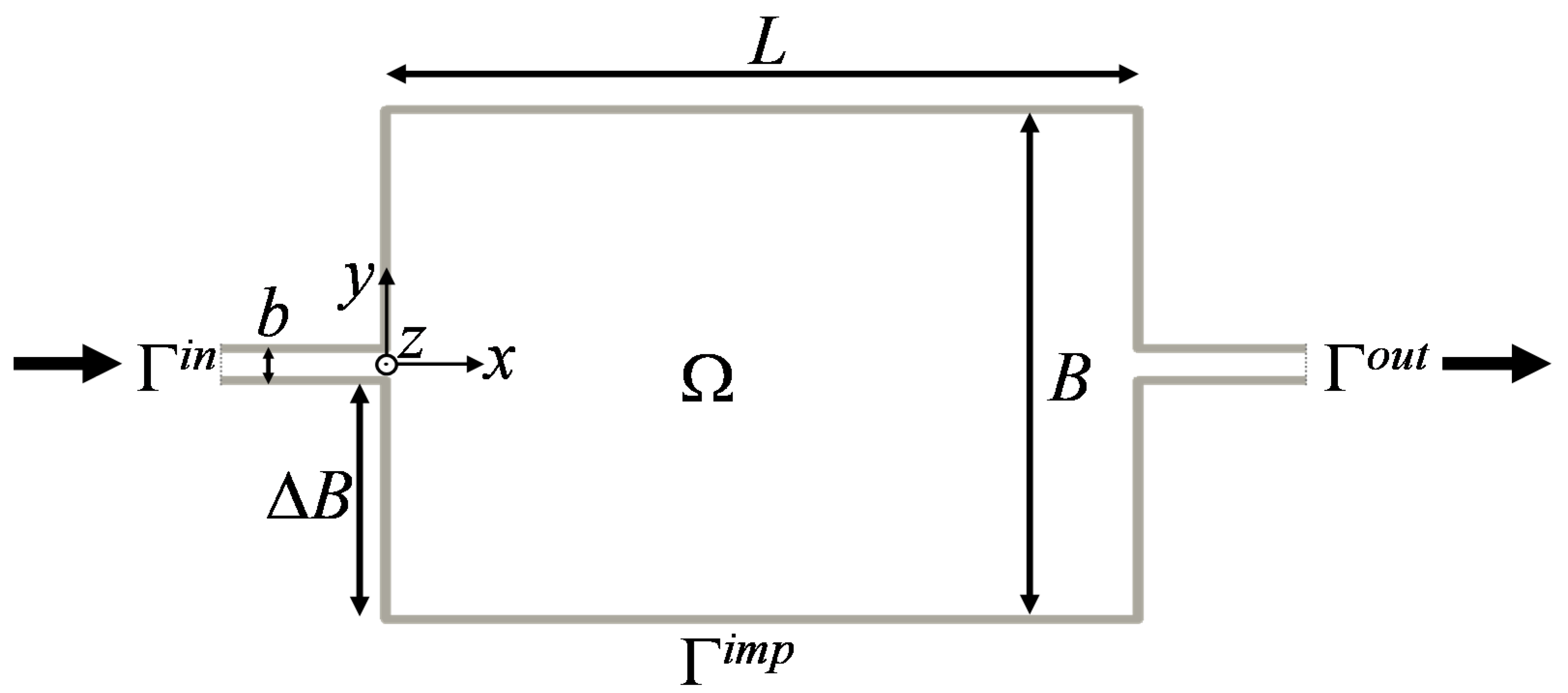
2.1. Characteristics of the Considered Reservoirs

In total, 10 cases of steady-state water flows in laboratory-scale rectangular shallow reservoirs of various sizes are considered (Figure 1 and

Table 2. Tested configurations.

Test ID	L (m)	B (m)	SF (−)	Type of Flow Pattern	Test ID in Camnasio et al. [18]
1	3	4	3.6	Detached jet (D)	5
2	4	3	5.8	Detached jet (D)	6
3	5	4	6.0	Near-transition (NT)	4
4	5.8	4	6.9	Near-transition (NT)	2
5	6	4	7.2	Reattached jet (R)	1
6	4	2	7.6	Reattached jet (R)	7
7	4	1	12.5	Reattached jet (R)	8
8	6	1	18.8	Reattached nearly-plug-flow (R-NPF)	9
9	6	0.75	24.0	Reattached nearly-plug-flow (R-NPF)	10
10	6	0.6	29.7	Reattached nearly-plug-flow (R-NPF)	11

). The geometric characteristics of the reservoirs and the hydraulic conditions are exactly the same as those analyzed by Camnasio et al. [18]. The reservoir bottom is smooth and horizontal, while the width of the inlet and outlet channels is kept constant and equal to b = 0.25 m (Figure 1). In the considered configurations, the reservoir width B varies between 0.6 m and 4 m, and the reservoir length L between 3 m and 6 m (Table 2). In all cases, the inlet and outlet channels are located on the reservoir centerline.

As shown by Dufresne et al. [14] and Goltsman and Saushin [29], the type of flow pattern developing in rectangular shallow reservoirs depends on the value of a so-called shape factor, SF, expressing the relative length of the reservoir compared to its expansion (ΔB = (B – b)/2) and to the width of the inlet channel: SF = L/(ΔB^0.6 b^0.4). Critical values of SF were determined by Dufresne et al. [14] based on laboratory experiments. A detached jet flowing straight from the inlet to the outlet is observed for relatively short reservoirs (SF < 6.2). In contrast, for longer reservoirs (SF > 6.8), the jet reattaches on either of the side-walls. In the case of particularly long reservoirs, a flow pattern close to plug flow is observed in the downstream portion of the reservoir. For 6.2 ≤ SF ≤ 6.8, a transition zone was reported, in which both detached and reattached flow patterns may occur.

The set of 10 configurations considered here (Table 2) covers the different types of steady flow patterns that can be observed in rectangular shallow reservoirs. In contrast, since the focus is set here on steady flow configurations, the case of meandering jets is not considered [21,30].

Considering that the reservoir bottom and walls are smooth is certainly a simplifying assumption. It is well known that bottom roughness may alter the flow pattern observed in such reservoirs, as shown by Choufi et al. [17]. Indeed, varying the roughness changes the relative importance of friction forces and other governing forces, such as horizontal shear. This effect is comparable to the influence of varying the flow shallowness, which leads to the definition of frictional and non-frictional regimes [30,31]. Nonetheless, the flow model used here was already shown to provide reasonable predictions for a broad range of flow types, covering both the non-frictional and frictional regimes [21].

Similarly, the bottoms of real-world reservoirs are generally not characterized by a uniform roughness and are not entirely flat, e.g., due to spatially varied sediment depositions. Again, the flow model used here is able to reproduce the effect of spatial variability in the reservoir bottom’s characteristics [19]. However, we stick here to simple flat and smooth reservoirs to highlight the main features of water age distribution as a function of the reservoir geometry.

2.2. Flow Model and Computed Flow Fields

The current study relies directly on the flow fields computed earlier by Camnasio et al. [18]. In their model, the ratio of the flow depth to the horizontal size of the reservoir (aspect ratio) was assumed to be sufficiently small that the vertical variations of all the variables, except pressure, may be ignored. Therefore, the shallow-water equations were used to compute the depth-averaged horizontal velocity, u, and the flow depth, H. These variables depend on the horizontal position vector x = (x, y), where x and y are Cartesian coordinates. The horizontal eddy viscosity and diffusivity are evaluated by means of a two-length-scale depth-averaged k–ε turbulence model, as described by Camnasio et al. [18].

The complete system of partial differential equations solved, coupling the shallow-water equations and the equations for k and ε, are written out in full by Camnasio et al. [18]. The numerical computations were performed on a Cartesian grid (spacing of 0.025 m), with a second-order accurate finite volume scheme implemented in the academic model WOLF 2D.

Although the aspect ratio of the reservoirs under study is small, so that it is generally appropriate to deal with depth-averaged variables, the occurrence of secondary currents (e.g., in curved portions of the jet or in recirculation cells) cannot be excluded completely. Such flow processes should be investigated based on a non-hydrostatic 3D flow model, which is out of the scope of the present research. Nonetheless, the validity of the model considered here for predicting horizontal flow fields in shallow reservoirs was repeatedly proven [18,19,21,32]. Particularly, the model assessment included a grid sensitivity analysis [32] based on the grid convergence index introduced by Roache et al. [33], as well as a demonstration that the model predicts accurately the velocity profiles in similar shallow reservoirs, as considered here [18,19]. Therefore, the validation of the flow model is not discussed further.

Examples of the computed flow fields are displayed in Figure 2, while the flow and eddy viscosity fields for the 10 considered configurations are provided in the Supplemental Material (Figures S1 and S2). The flow patterns are in agreement with the empirical criteria of Dufresne et al. [14]. In Tests 1 and 2, the jet is detached (Figure 2a), whereas a reattached jet is found in Tests 5, 6 and 7 (Figure 2c). Tests 8, 9 and 10 also involve a reattached jet; but in these cases, the reservoirs are so long that a nearly-plug-flow is observed in the downstream part of the reservoir (Figure 2d). Tests 3 and 4 are very close to the empirical transition zone; but for both of them, the computed flow fields show a detached jet (Figure 2b) [18].

2.3. Water Age Distribution Function

The age of a water particle is defined as the time elapsed since it entered the domain of interest by crossing its inlet. However, the evolution of a single particle is rather irrelevant. A sufficiently large number of them must be considered. Accordingly, the water particles present at a given instant in an elemental control volume are unlikely to have followed the same paths to reach it. In other words, they are likely to have different ages, hence the need to introduce the histogram of their ages.

Hereinafter, the domain of interest (the reservoir under study) is denoted by Ω. Its boundary, Γ, is made up of three parts (Figure 1), the inlet, outlet and impermeable boundaries, which are referred to as Γⁱⁿ, Γ^out and Γ^imp, respectively.

The so-called age distribution function, the core variable of the age theory resorted to herein [28,34], will help us assess the variability of the water particles’ travel times. To introduce this function, the first step consists in defining an elemental control domain (δΩ) well suited to the depth-averaged approach. The corresponding space coordinate intervals are [x, x + δx] and [y, y + δy], where the space increments are such that δx, δy→0. The volume of δΩ is δV (x) = δx δy H (x). The age distribution function is denoted as c (x, τ), where the independent variable τ is the age (0 ≤ τ ≤ ∞). In accordance with Delhez et al. [28], the following definition is adopted: in the abovementioned elemental control domain, the mass of the water whose age lies in the interval [τ, τ + δτ] tends to ρ c (x, τ) δV δτ in the limit δV, δτ → 0 (with ρ as the water density). The physical dimension of the age distribution function c (x, τ) is time⁻¹.

From mass budget considerations, Delhez et al. [28] derived the general equation governing the age distribution function of any constituent of a fluid mixture, taking into account advection, diffusion and reactive processes. Specifically, the mass flux evaluated in the age direction is due to ageing, i.e., the fact that the age of every water particle increases at the same pace as time progresses. Here, a simplified version thereof was used because the focus is set on steady-state and depth-averaged variables. In addition, water is regarded as a passive tracer (i.e., no reactions are to be considered). Accordingly, the water age distribution function obeys:

$$\frac{\partial (Hc)}{\partial \tau }=-\nabla ·(Hcu-HK·\nabla c)$$

(1)

where K(x) denotes the diffusivity tensor, which must be symmetric and positive definite. Equation (1) is of a parabolic nature. Formally, Equation (1) is similar to an “evolution” equation, in which the independent variable τ plays a role equivalent to that of time in a classical advection–diffusion equation. A detailed derivation of this equation, as well as some of the mathematical properties of its solution, may be found in Deleersnijder and Dewals [35].

As pointed out above, the age is defined as the time elapsed since entering the shallow reservoir under study. Therefore, in the domain interior Ω, no water particle has zero age, yielding the “initial condition” (i.e., for τ = 0):

$$c(x,0)=0$$

(2)

The age of a water particle is set to zero at the moment it enters the domain through inlet Γⁱⁿ. The incoming-flux condition reads [36]:

$${\left[(Hcu-HK·\nabla c)·n\right]}_{x\in {\mathsf{\Gamma }}^{in}}={\left[H(u·n)\delta (\tau -0)\right]}_{x\in {\mathsf{\Gamma }}^{in}}$$

(3)

where δ is the Dirac delta function. On the inlet, not all the water particles have zero age due to diffusion. A tailgate is placed at the downstream end of the outlet channel, so that the fluxes there are assumed to be of an advective nature. This leads to the boundary condition:

$${\left[(HK·\nabla c)·n\right]}_{x\in {\mathsf{\Gamma }}^{out}}=0$$

(4)

On the impermeable boundary, a no-flux condition is prescribed,

$${\left[(HCu-HK·\nabla c)·n\right]}_{x\in {\mathsf{\Gamma }}^{imp}}=0$$

(5)

which, given the definition of the impermeable boundary, reduces to this simpler formulation:

$${\left[(-HK·\nabla c)·n\right]}_{x\in {\mathsf{\Gamma }}^{imp}}=0$$

(6)

2.4. Mathematical Properties of the Mean Water Age

The partial differential problem constituted, of Equation (1) and auxiliary conditions (2)–(4) and (6), ensures a number of key properties of the age distribution function c (x, τ), namely c (x, τ) is non negative, τ c (x, τ) tends to zero in the limit τ→ ∞, and c (x, τ) satisfies the following integral constraint expressing that the concentration of water C(x) is equal to unity at any location in the domain [28]:

$$C(x)={\displaystyle \underset{0}{\overset{\infty }{\int }}c(x,\tau )d\tau }=1$$

(7)

In accordance with Delhez [28], the mean age of the water at location x is defined as the first-order moment of the water age distribution function:

$$a(x)={\displaystyle \underset{0}{\overset{\infty }{\int }}\tau c(x,\tau )}d\tau$$

(8)

This expresses the so-called age-averaging hypothesis [34].

A steady-state equation governing the mean age can be derived by taking the first-order moment of Equations (1)–(4) and (6). However, in this research, this equation was not solved directly, but the mean age was derived from the computation of the age distribution function c (x, τ). The obtained values of a(x) exhibit the following properties [35]:

• The solution is unique;
• a(x) is non-negative;
• The value of the mean age on the incoming boundary is not zero, unless diffusion is zero. Indeed, on Γⁱⁿ, there is a mixture of water particles that are entering the domain and particles that have been moving for some time in the domain and were brought back to the incoming boundary by diffusion;
• The maximum of the mean age is not necessarily on the outgoing boundary Γ^out, but it may be located inside the domain of interest. This contrasts with a one-dimensional setting, in which the maximum of mean age occurs at the outgoing boundary because there is only one path from the reservoir inlet to the outlet;
• On the outgoing boundary Γ^out, the average value of the mean age satisfies:

$$\begin{array}{l}\overline{\xi }=\frac{1}{S^{out}}{\displaystyle \underset{{\mathsf{\Gamma }}^{out}}{\int }H(x)a(x)}d{\mathsf{\Gamma }}^{out}=\frac{V}{Q}-{\displaystyle \underset{{\mathsf{\Gamma }}^{out}}{\int }H(x)\left[a(x)-\overline{\xi }\right]u·n}d{\mathsf{\Gamma }}^{out},\\ \mathrm{with}{S}^{out}={\displaystyle \underset{{\mathsf{\Gamma }}^{out}}{\int }H(x)}d{\mathsf{\Gamma }}^{out};V={\displaystyle \underset{\Omega }{\int }H(x)}d\Omega ;Q={\displaystyle \underset{{\mathsf{\Gamma }}^{out}}{\int }H(x)u·n}d{\mathsf{\Gamma }}^{out}.\end{array}$$

(9)

where V and Q denote the volume of the water contained in the reservoir and the volumetric flow rate entering (or leaving) it, respectively. This underscores the importance of the ratio V/Q, which may be regarded as the order of magnitude of the mean age on the outgoing boundary (also called transit time). In a one-dimensional setting in a steady state, the mean age at the outgoing boundary is equal to V/Q irrespective of the diffusivity and cross-sectional area profiles.

2.5. Computational Procedure

From a computational point of view, obtaining the age distribution function c(x, τ) from the partial differential problem (5)–(9) is unlikely to be the optimal method due to the Dirac delta impulse prescribed as incoming boundary condition. Therefore, as proposed earlier [37], an alternate approach was set up here. In line with the theory of linear system dynamics, stating that the impulse response can be evaluated as the derivative of the step response, i.e., by prescribing a step function as inflowing boundary condition instead of the Dirac delta impulse. The step response is of course much easier to compute numerically than the impulse response.

As such, two steps were followed to evaluate the age distribution function. First, the step response, b(x, τ), was obtained by solving the following partial differential problem, which is akin to a standard advection–diffusion problem (in which τ plays a role equivalent to that of the time):

$$\frac{\partial (Hb)}{\partial \tau }=-\nabla ·\left(Hbu-HK·\nabla b\right)$$

(10)

$$b(x,0)=0$$

(11)

with

$${\left[(Hbu-HK·\nabla b)·n\right]}_{x\in {\mathsf{\Gamma }}^{in}}={\left[Hu·n\right]}_{x\in {\mathsf{\Gamma }}^{in}}$$

(12)

$${\left[(HK·\nabla b)·n\right]}_{x\in {\mathsf{\Gamma }}^{out}\cup {\mathsf{\Gamma }}^{imp}}=0$$

(13)

Here, the incoming flux is independent of τ instead of a Dirac delta function in problem (5)–(9). In the computations, an isotropic eddy diffusivity (K = κ I) was used, with the value of κ taken as equal to the eddy viscosity.

In a second step, the age distribution function c (x, τ) was computed by evaluating the derivative of b (x, τ):

$$c(x,\tau )=\frac{\partial }{\partial \tau }b(x,\tau )$$

(14)

In line with Equation (7), the cumulative distribution function b (x, τ) tends to unity for τ → ∞. Finally, once the age distribution function is computed, the mean water age a(x) can be evaluated thanks to Equation (8). Note that an alternate approach consists in simulating the problem in Laplace space [38].

3. Results

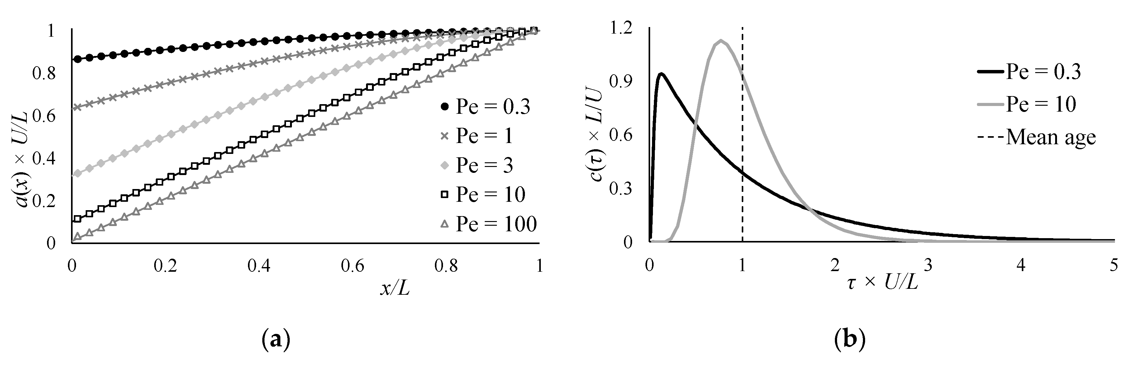
3.1. Model Verification: Prismatic Channel

For the purpose of model verification, the age profile in a one-dimensional setting, for which an analytical solution is available, was first computed. A prismatic rectangular channel of length L = 1 m and unit width is considered, in which the section-averaged flow velocity is U = 1 m/s. In a steady state, the value of U is uniform along the reservoir. A uniform along-flow diffusivity K is assumed. The age is

$$a(x)=\frac{L}{U}\left(\frac{x}{L}+\frac{1-e^{-Pe(1-x/L)}}{Pe}\right)=\frac{V}{Q}\left(\frac{x}{L}+\frac{1-e^{-Pe(1-x/L)}}{Pe}\right)$$

(15)

where Pe = U L/K is the Peclet number.

In Figure 3a, this analytical solution is compared to the water age computed from Equations (10)–(14) and Equation (8). By varying the value of the diffusivity K, this comparison was performed for Peclet numbers ranging over nearly three orders of magnitude (from 0.3 up to 100). The computations and the analytical solution match very well. The results for smaller values of K (i.e., Pe lower than 100) cannot be distinguished visually from those obtained with Pe = 100. Hence they are not represented.

Note that the mean water age is indeed different from zero at the inflow boundary, as emphasized in Section 2.4. Moreover, the smaller the relative importance of diffusion is (i.e., the larger the Peclet number), the smaller the mean water age on the inflowing boundary will be.

Another remarkable feature of the results is that they all converge towards the same value, a(L) = L/U = V/Q, at the exit side, irrespective of the value of the Peclet number. However, a benefit of applying our model is that it gives access not only to the mean water age a(x), but also to the age distribution function c(x, τ), for which an analytical solution written in closed form is not available. Figure 3b reveals that, although the mean age a(L) is the same for various values of Peclet number, the age distribution functions differ substantially—the stronger the diffusion, the more the distribution is skewed towards large values of age, but nonetheless smaller values of age are more frequent.

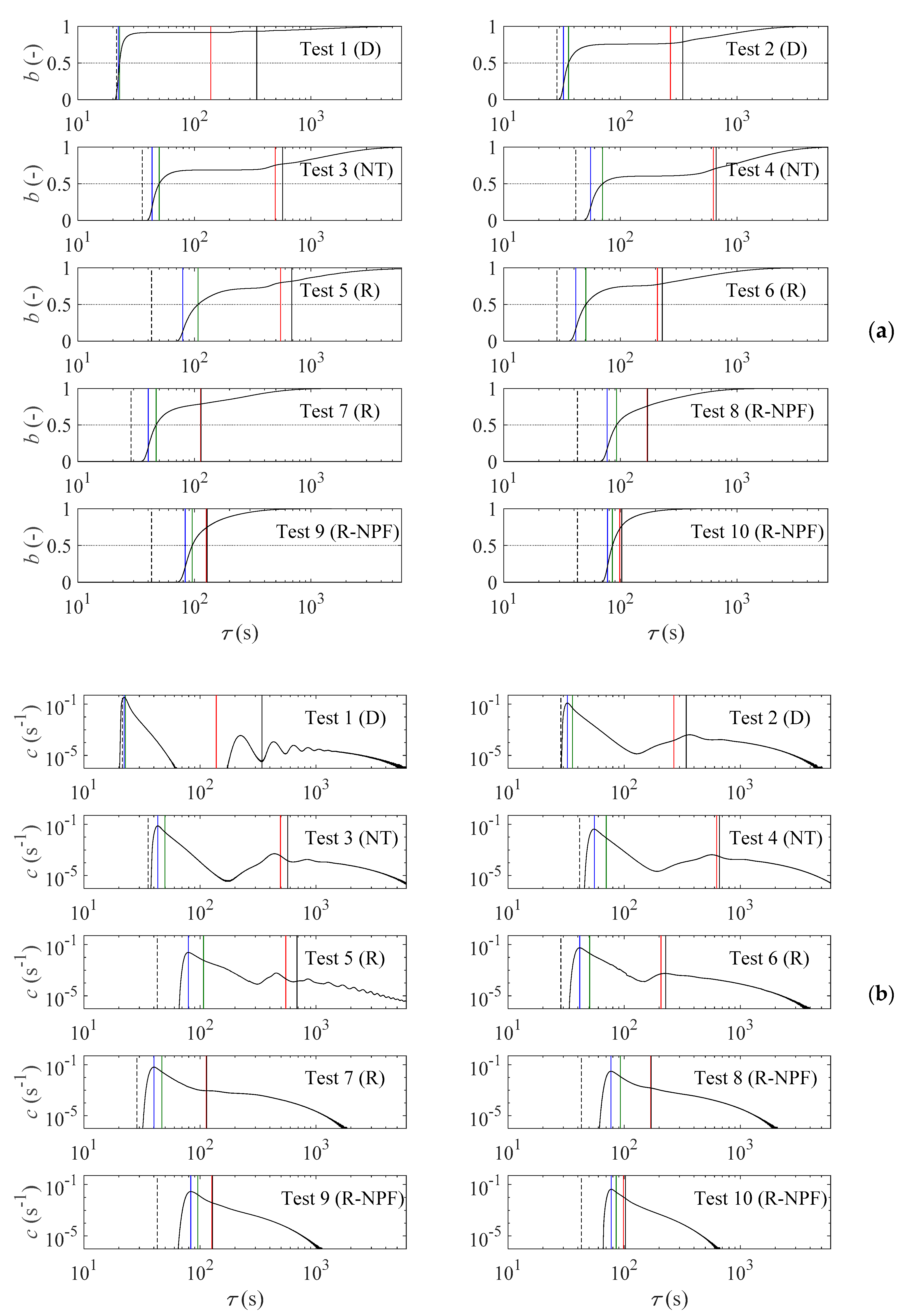
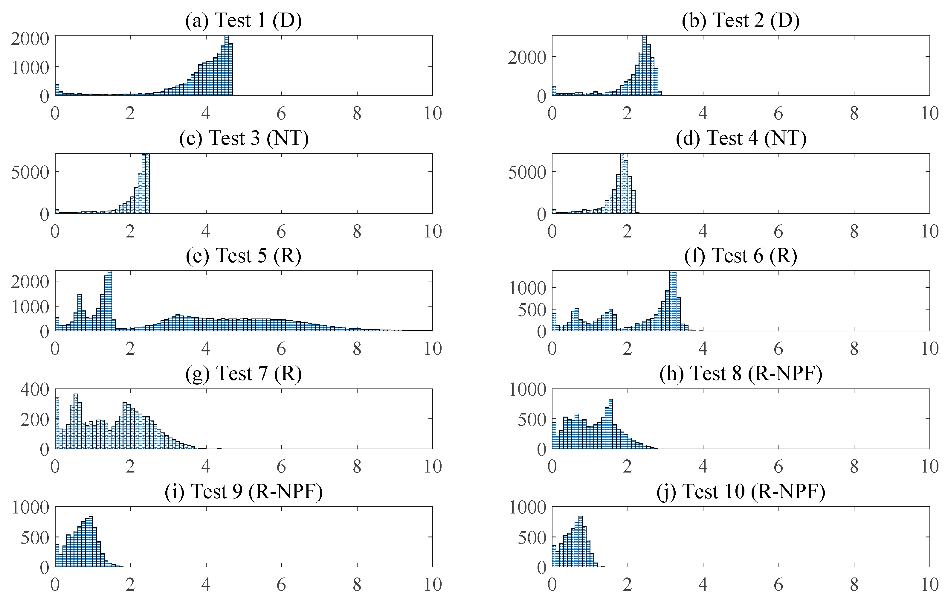
3.2. Distribution of Water Age at Reservoir Outlet

The two-step procedure described in Section 2.5 was applied to all the configurations listed in Table 2. Examples of step responses computed for Test 5 and Test 6 are shown in Figures S3 and S4 in the Supplemental Material. Here, the water age distribution on the centerline of the reservoir outlet section is first examined. For all configurations, the water age distribution and cumulative distribution at the reservoir outlet are shown in logarithmic scale in Figure 4. The following observations can be made:

• In the nearly-plug-flow configurations (Tests 8, 9 and 10), the water age distribution at the outlet is unimodal, but strongly skewed towards the higher values of τ;
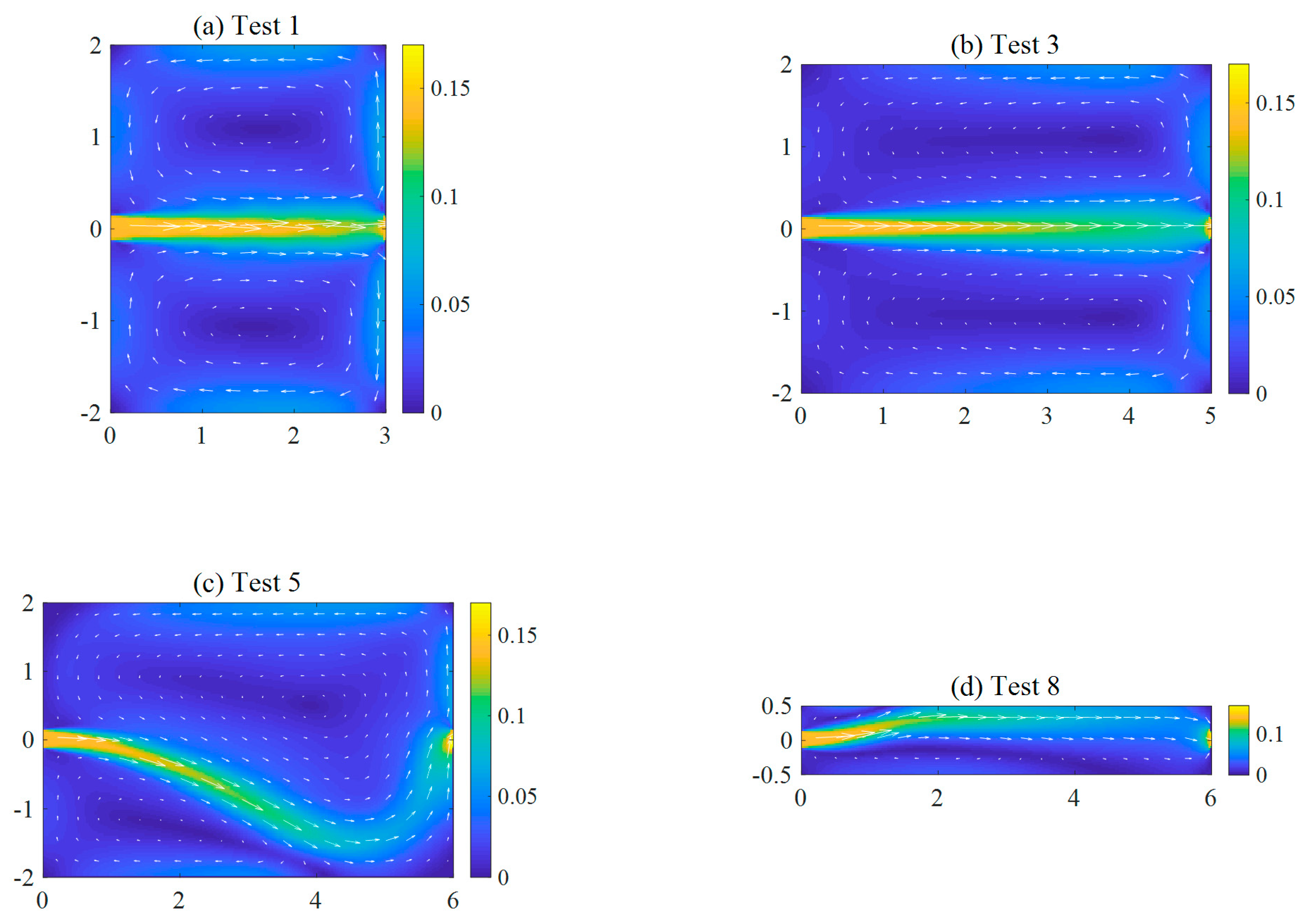
• Looking sequentially at the results obtained for Tests 7, 6 and 5, all corresponding to configurations with a reattached jet, it appears that the water age distribution at the outlet shifts gradually from a unimodal to a bimodal distribution;
• In all cases with a detached jet, the water age distribution at the outlet is bimodal (Tests 4, 3 and 2), or even multimodal in the case of Test 1.

The occurrence of bi- and multimodal distributions is attributed to the large flow recirculations, which develop on both sides of the main jet in the case of a reattached jet (Tests 6 and 5) and, to an even greater extent, in the case of detached jets. The water reaching the reservoir outlet contains particles which have followed distinct pathways: a portion of them followed the main jet (fast route), whereas others remained trapped for some time in the large flow recirculations (slow route). Since the computed age distributions are finely discretized as a function of τ, we discard the hypothesis that the multimodal nature of the computed distributions is a bias from numerical computation. Overall, these results show that a reduced number of indicators (e.g., mean age and standard deviation) would not be sufficient to reflect the complexity and variety of the actual water age distributions.

Figure 4 also displays the mode, the median and the mean of water age. These quantities are compared in scatter plots given in Figures S5 and S6 in the Supplemental Material. In all configurations, the mean age exceeds the median age, which in turn exceeds the mode of the age distribution. The median age is generally 5% to 35% larger than the mode of the distribution. The mode and the median age are the closest to each other in the configurations with a detached jet (Tests 1 and 2), with differences not exceeding 5% to 10%.

The mean age differs considerably from the mode and the median age. Indeed, the mean ages are found to be up to ten times higher than the corresponding median values. The tests with particularly large flow recirculations lead to the largest differences between mean and median age. This is attributed to the particularly high age of the water particles reaching the outlet after staying trapped for some time in those recirculations. This is also perfectly consistent with the considerable positive skewness of the corresponding water age distributions. In contrast, in the nearly-plug-flow configurations (Tests 8, 9 and 10), the mean age exceeds the median age by no more than a factor of two.

Finally, Figure 4 also displays two characteristic times which are straightforward to derive from the reservoir geometry and the boundary conditions:

• V/Q, which would correspond to the transit time through the reservoir in the case of a perfect plug flow all over the reservoir;
• L/(Q/Sⁱⁿ), would be equal to the transit time through the reservoir if the jet at the inlet was not diffused at all in the crosswise direction.

The truth is of course in-between these two extremes. Indeed, Figure 4 reveals that the characteristic times V/Q and L/(Q/Sⁱⁿ) tend to provide an envelope for the mode, median and mean ages. In the case of nearly-plug-flow, the characteristic time V/Q is found to approximate remarkably well the mean water age, with overestimations of no more than 5%. Furthermore, in one case of a reattached jet in a particularly elongated reservoir (Test 7), V/Q matches the mean age with a difference of less than 1%. In all other configurations, V/Q remains a reasonable approximation for the mean age, with overestimations of no more than 22%. Only in the case corresponding to a detached jet in a relatively wide basin (Tests 1), V/Q overestimates the mean age by a factor 2.5.

The second characteristic time, L/(Q/Sⁱⁿ), is generally between 1.5 and 2.5 times smaller than the median age and the mode of the age distribution. Only in the configurations with a detached jet (Tests 1 and 2), L/(Q/Sⁱⁿ) approximates well the mode and the median age, with an underestimation of the order of 10% to 20% only. Note that only for Test 1, a small portion of the water particles show a transit time even smaller than the characteristic value L/(Q/Sⁱⁿ). This results from the velocity profile over the jet cross-section. Indeed, the central part of the jet at the inlet has a velocity higher than Q/Sⁱⁿ. In all other cases, the characteristic time L/(Q/Sⁱⁿ) substantially underestimates the actual mode, median and mean values of the age distribution.

Consequently, L/(Q/Sⁱⁿ) appears as a useful time scale for the configurations with a detached jet flowing directly from the inlet to the reservoir outlet (Tests 1 and 2), whereas the characteristic time scale V/Q approximates well the mean age at the outlet in the case of elongated reservoirs with nearly-plug-flow conditions (Tests 8, 9 and 10) or close to (Tests 6 and 7).

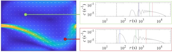
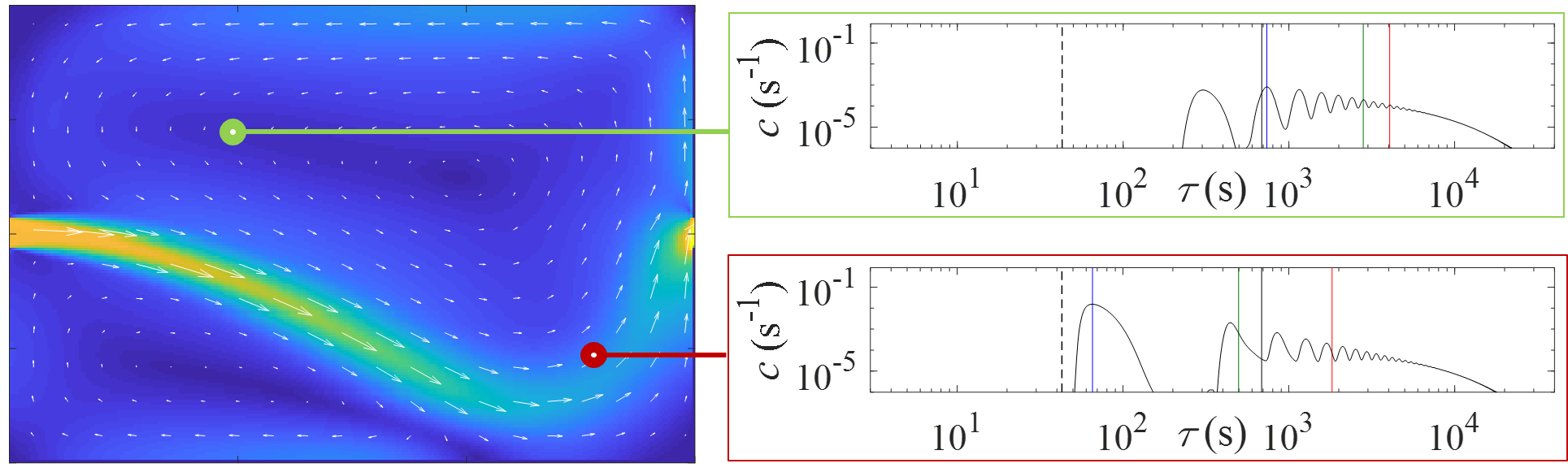
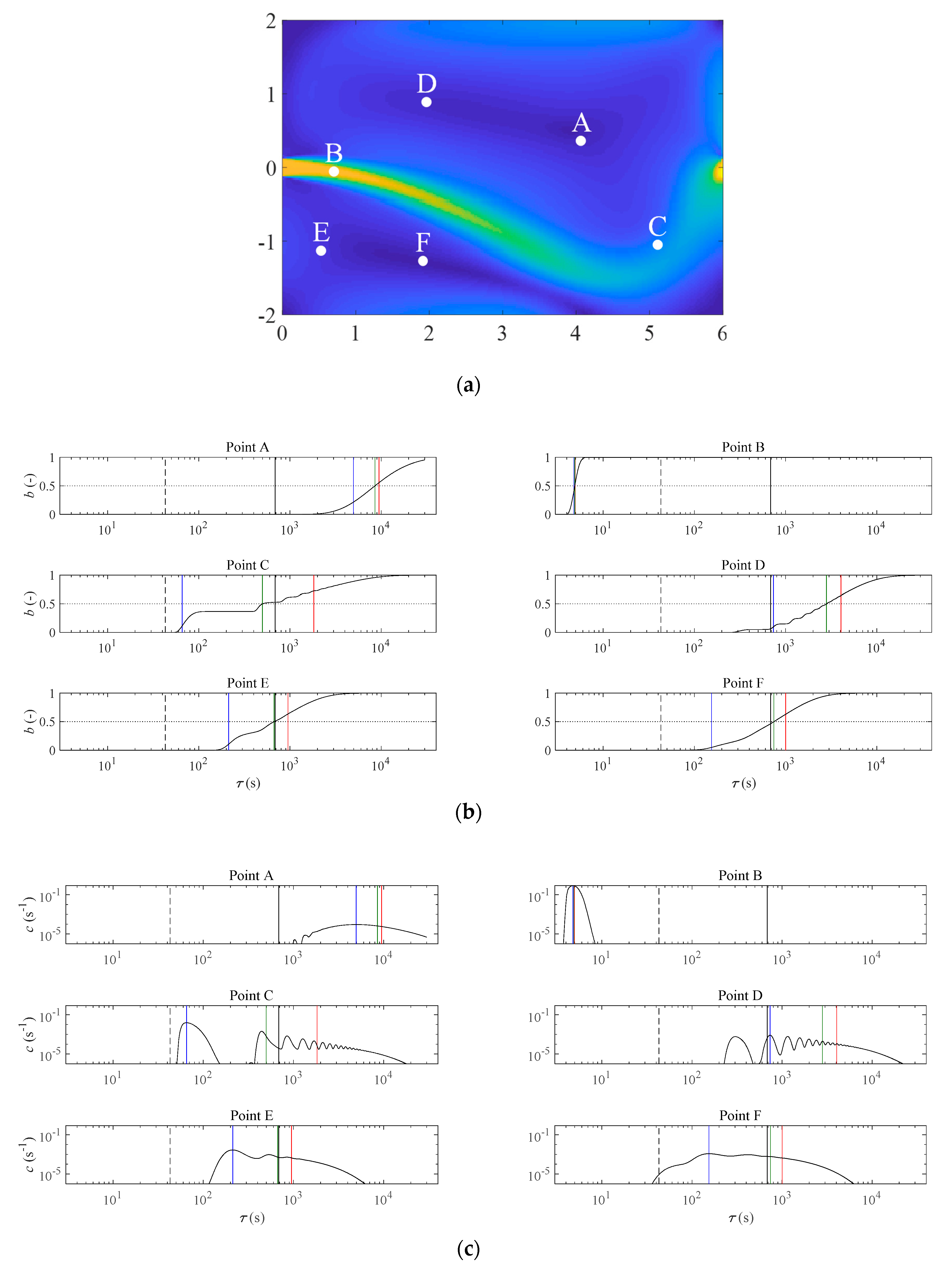
3.3. Distribution of Water Age within the Reservoirs

Here, the water age distributions at specific locations within the reservoir are analyzed. A configuration with a reattached jet, namely Test 5, is considered. It shows a particularly complex flow pattern. The corresponding water age distributions are displayed in Figure 5. Similar results for Test 6 are displayed in Figure S7 in the Supplemental Material.

In both configurations (Tests 5 and 6), Point B is located on the centerline of the main jet, at a distance from the reservoir inlet equal to 3.5 times the inlet width. The water age distribution at this location is fairly simple, unimodal and with a slight skewness towards the greater water ages. Unsurprisingly, the mean, median and mode for age are all very close, as the water particles at Point B have all followed a similar route. Indeed, these three quantities differ from each other by no more than 1% to 3% in Test 5, and 2% to 5% in Test 6. This contrasts strongly with the results obtained at the reservoir outlet (Section 3.2) and at other locations within the reservoir, which all show much “wider” age distributions.

Points E and F are located in the smaller recirculation zone on the right side of the main jet. These distributions are multimodal, reflecting the coexistence in these recirculations of water particles that have followed distinct paths, such as either coming “directly” from the reservoir inlet or having been temporarily “trapped” in the recirculation zone.

The results are to a great extent similar at Point D, which is located in the larger recirculation on the left side of the jet. In the case of Test 5, the water age distribution at Point D shows multiple peaks.

Points A are situated close to the center of the larger recirculation on the left side of the jet. The corresponding distributions are also multimodal, with a particularly large “spreading”, revealing the coexistence of water particles characterized by ages ranging over at least two orders of magnitude. Note that, despite the long computation time dedicated to the simulation, the water age distribution captured by the computational model at Point A in the case of Test 5 is not complete. However, this does not undermine the conclusions, since the key features of the distribution are well captured.

Finally, Point C is located along the jet, at a distance of about seven outlet widths from the reservoir outlet. The water age distribution at this location approaches the water age distribution at the reservoir outlet.

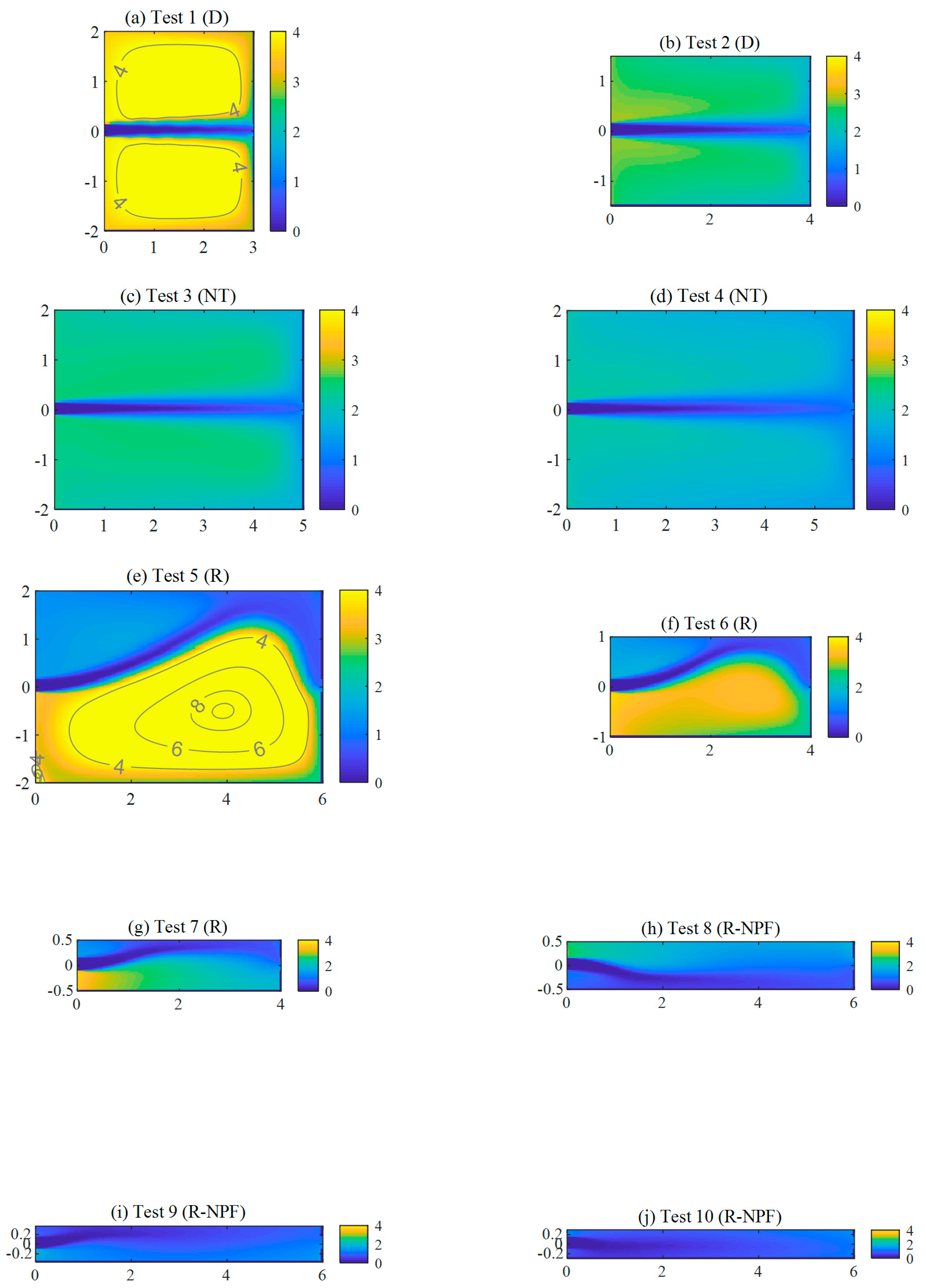
3.4. Mean Age in the Reservoirs

Figure 6 represents the spatial distribution of the mean water age a, scaled by the characteristic time V/Q introduced in Section 3.2. This non-dimensional mean water age takes maximum values in the large flow recirculations, irrespective of whether the main jet is reattached (e.g., Test 5) or not (e.g., Test 1).

The maximum values of the non-dimensional water age tend not to exceed a value close to four, except in Test 5. In this case, the non-dimensional mean water age reaches about 20 in the core of the large flow recirculation.

For each test, Figure 7 shows a histogram of the computed non-dimensional mean water ages a/(V/Q) across the 10 considered reservoirs. The displayed range of a/(V/Q) does not extend beyond 10 because, although existing for Test 5, the number of values above 10 is so small that they are not visible in the graphs.

In the most elongated reservoir (Test 10), the values a/(V/Q) are mostly below unity, in accordance with Deleersnijder and Dewals [35]. In the other tests corresponding to nearly-plug-flow (Tests 8 and 9), the maximum values of a/(V/Q) remain between 1 and 3.

In the cases with a reattached jet (Tests 5, 6 and 7), the coexistence of fast and slow routes is clearly reflected in the histograms of a/(V/Q). Indeed, two groups of values of a/(V/Q) can be distinguished in the histograms: one corresponding to a/(V/Q) > 2 (in the larger flow recirculations) and another one to a/(V/Q) < 2 (main jet and smaller recirculation), consistently with Figure 6e–g.

The other tests also show a distinctive bimodal pattern in the histograms of a/(V/Q). The most populated mode shows values for a/(V/Q) of the order of 3 to 5, and corresponds to the larger flow recirculations on either sides of the main jet. Besides this, a smaller peak can be seen for very small values of a/(V/Q), corresponding to the main jet whose characteristic time is closer to L/(Q/Sⁱⁿ) than V/Q.

4. Conclusions

In this research, the complexity of the distribution function of water age within shallow reservoirs of simple rectangular geometry is highlighted. These water age distribution functions are often multimodal as a result of the coexistence of fast and slow routes within the reservoir. The existence of distinct routes results from various large-scale turbulent structures developing in such reservoirs. As a result, a limited number of statistical values (e.g., mean and standard deviation of age) would fail to reflect the complexity of the actual water age distributions in such reservoirs.

To evaluate the water age distribution, the “step response” was first computed and, next, the result was derived to obtain the age distribution function. This procedure was applied to 10 configurations of rectangular shallow reservoirs, for which steady flow fields, previously computed with a validated model, were readily available. They involve a variety of flow patterns, including detached or reattached jets, large flow recirculations and nearly-plug-flow.

Two characteristic time scales are worth considering V/Q (with V the reservoir volume and Q the inflow discharge) and L/(Q/Sⁱⁿ) (with L the reservoir length and Sⁱⁿ the inlet cross-section), and their relative merits are discussed as a function of the reservoir dimensions. The former time scale provides an estimate of practical relevance for the mean water age at the outlets of elongated reservoirs, whereas the latter is a useful proxy for the mode and the median age at the outlets of relatively short reservoirs. The spatial distribution of the mean age within the reservoir is shown to vary strongly with the reservoir’s geometry, and these variations are attributed to characteristics of the flow fields.

The insights provided by this numerical research may prove important for guiding the optimal geometric and hydraulic design of reservoirs used for water storage, for trapping sediments or as service reservoirs. Indeed, the prediction of water age and its distribution enables the pinpointing of issues such as preferential sedimentation or uneven disinfection time in the case of service reservoirs. Specifically, knowing the water age and its distribution enables a comparison of the corresponding time scales to other time scales of relevance, such as the characteristic time of sedimentation (as a function of the settling velocity of the sediment particles of interest), or the time during which a disinfectant remains active in a service reservoir [11]. Comparing these time scales for a range of design options enables assessing which are the most favorable geometric and hydraulic design choices. Maintenance costs may also be cut down thanks to a deeper understanding of water age distribution in such reservoirs.

Future research should focus on computing not only the water age distribution, but also the age of sediments transported either as bed load or as suspended load [39,40]. Comparing the results of our Eulerian modeling framework with those of a Lagrangian approach [41,42], including stochastic terms to represent the impact of turbulent diffusion [43,44,45], would lead to valuable insights into the relative performance of each technique. Moreover, our diagnostic tools should be extended to accommodate 3D flow fields in shallow reservoirs [8,20,46], since three-dimensional turbulent structures and secondary currents are likely to alter the distribution of water age. Finally, examining the performances of alternate turbulence closures would be another valuable piece of further research.

References

1. Brink, I.C.; Kamish, W. Associations between stormwater retention pond parameters and pollutant (Suspended solids and metals) removal efficiencies. Water SA 2018, 44, 45–53. [Google Scholar] [CrossRef] [Green Version]
2. Dominic, J.A.; Aris, A.Z.; Sulaiman, W.N.A.; Tahir, W.Z.W.M. Discriminant analysis for the prediction of sand mass distribution in an urban stormwater holding pond using simulated depth average flow velocity data. Environ. Monit. Assess. 2016, 188, 1–15. [Google Scholar] [CrossRef]
3. Guzman, C.B.; Cohen, S.; Xavier, M.; Swingle, T.; Qiu, W.; Nepf, H. Island topographies to reduce short-circuiting in stormwater detention ponds and treatment wetlands. Ecol. Eng. 2018, 117, 182–193. [Google Scholar] [CrossRef] [Green Version]
4. MoayeriKashani, M.; Hin, L.S.; Ibrahim, S. Experimental investigation of fine sediment deposition using particle image velocimetry. Environ. Earth Sci. 2017, 76, 655. [Google Scholar] [CrossRef]
5. Sebastian, C.; Becouze-Lareure, C.; Lipeme Kouyi, G.; Barraud, S. Event-based quantification of emerging pollutant removal for an open stormwater retention basin—Loads, efficiency and importance of uncertainties. Water Res. 2014, 72, 239–250. [Google Scholar] [CrossRef] [PubMed]
6. Sonnenwald, F.; Guymer, I.; Stovin, V. Computational fluid dynamics modelling of residence times in vegetated stormwater ponds. Proc. Inst. Civ. Eng. Water Manag. 2018, 171, 76–86. [Google Scholar] [CrossRef]
7. Stovin, V.R.; Saul, A.J. Computational fluid dynamics and the design of sewage storage chambers. Water Environ. J. 2000, 14, 103–110. [Google Scholar] [CrossRef]
8. Isenmann, G.; Dufresne, M.; Vazquez, J.; Mose, R. Bed turbulent kinetic energy boundary conditions for trapping efficiency and spatial distribution of sediments in basins. Water Sci. Technol. 2017, 76, 2032–2043. [Google Scholar] [CrossRef]
9. Liu, X.; Xue, H.; Hua, Z.; Yao, Q.; Hu, J. Inverse calculation model for optimal design of rectangular sedimentation tanks. J. Environ. Eng. 2013, 139, 455–459. [Google Scholar] [CrossRef]
10. Tarpagkou, R.; Pantokratoras, A. CFD methodology for sedimentation tanks: The effect of secondary phase on fluid phase using DPM coupled calculations. Appl. Math. Model. 2013, 37, 3478–3494. [Google Scholar] [CrossRef]
11. Zhang, J.-M.; Lee, H.P.; Khoo, B.C.; Peng, K.Q.; Zhong, L.; Kang, C.-W.; Ba, T. Shape effect on mixing and age distributions in service reservoirs. J. Am. Water Works Assoc. 2014, 106, E481–E491. [Google Scholar] [CrossRef]
12. Oca, J.; Masalo, I. Design criteria for rotating flow cells in rectangular aquaculture tanks. Aquac. Eng. 2007, 36, 36–44. [Google Scholar] [CrossRef] [Green Version]
13. Camnasio, E.; Orsi, E.; Schleiss, A. Experimental study of velocity fields in rectangular shallow reservoirs. J. Hydraul. Res. 2011, 49, 352–358. [Google Scholar] [CrossRef] [Green Version]
14. Dufresne, M.; Dewals, B.J.; Erpicum, S.; Archambeau, P.; Pirotton, M. Classification of flow patterns in rectangular shallow reservoirs. J. Hydraul. Res. 2010, 48, 197–204. [Google Scholar] [CrossRef]
15. Kantoush, S.A.; De Cesare, G.; Boillat, J.L.; Schleiss, A.J. Flow field investigation in a rectangular shallow reservoir using UVP, LSPIV and numerical modelling. Flow Meas. Instrum. 2008, 19, 139–144. [Google Scholar] [CrossRef]
16. Peltier, Y.; Erpicum, S.; Archambeau, P.; Pirotton, M.; Dewals, B. Experimental investigation of meandering jets in shallow reservoirs. Environ. Fluid Mech. 2014, 14, 699–710. [Google Scholar] [CrossRef]
17. Choufi, L.; Kettab, A.; Schleiss, A.J. Bed roughness effect on flow field in rectangular shallow reservoir. [Effet de la rugosité du fond d’un réservoir rectangulaire à faible profondeur sur le champ d’écoulement]. Houille Blanche 2014, 5, 83–92. [Google Scholar]
18. Camnasio, E.; Erpicum, S.; Archambeau, P.; Pirotton, M.; Dewals, B. Prediction of mean and turbulent kinetic energy in rectangular shallow reservoirs. Eng. Appl. Comput. Fluid Mech. 2014, 8, 586–597. [Google Scholar] [CrossRef] [Green Version]
19. Camnasio, E.; Erpicum, S.; Orsi, E.; Pirotton, M.; Schleiss, A.J.; Dewals, B. Coupling between flow and sediment deposition in rectangular shallow reservoirs. J. Hydraul. Res. 2013, 51, 535–547. [Google Scholar] [CrossRef] [Green Version]
20. Esmaeili, T.; Sumi, T.; Kantoush, S.A.; Haun, S.; Rüther, N. Three-dimensional numerical modelling of flow field in shallow reservoirs. Proc. Inst. Civ. Eng. Water Manag. 2016, 169, 229–244. [Google Scholar] [CrossRef] [Green Version]
21. Peltier, Y.; Erpicum, S.; Archambeau, P.; Pirotton, M.; Dewals, B. Can meandering flows in shallow rectangular reservoirs be modeled with the 2D shallow water equations? J. Hydraul. Eng. 2015, 141, 04015008. [Google Scholar] [CrossRef]
22. Peng, Y.; Zhou, J.G.; Burrows, R. Modeling free-surface flow in rectangular shallow basins by using lattice boltzmann method. J. Hydraul. Eng. 2012, 137, 1680–1685. [Google Scholar] [CrossRef]
23. Schleiss, A.J.; Franca, M.J.; Juez, C.; De Cesare, G. Reservoir sedimentation. J. Hydraul. Res. 2016, 54, 595–614. [Google Scholar] [CrossRef]
24. Bolin, B.; Rodhe, H. A note on the concepts of age distribution and transit time in natural reservoirs. Tellus 1973, 25, 58–62. [Google Scholar] [CrossRef]
25. Monsen, N.E.; Cloern, J.E.; Lucas, L.V.; Monismith, S.G. A comment on the use of flushing time, residence time, and age as transport time scales. Limnol. Oceanogr. 2002, 47, 1545–1553. [Google Scholar] [CrossRef] [Green Version]
26. Takeoka, H. Fundamental concepts of exchange and transport time scales in a coastal sea. Cont. Shelf Res. 1984, 3, 311–326. [Google Scholar] [CrossRef]
27. Persson, J. The hydraulic performance of ponds of various layouts. Urban Water 2000, 2, 243–250. [Google Scholar] [CrossRef] [Green Version]
28. Delhez, E.J.M.; Campin, J.-M.; Hirst, A.C.; Deleersnijder, E. Toward a general theory of the age in ocean modelling. Ocean Model. 1999, 1, 17–27. [Google Scholar] [CrossRef] [Green Version]
29. Goltsman, A.; Saushin, I. Flow pattern of double-cavity flow at high Reynolds number. Phys. Fluids 2019, 31, 065101. [Google Scholar] [CrossRef]
30. Peltier, Y.; Erpicum, S.; Archambeau, P.; Pirotton, M.; Dewals, B. Meandering jets in shallow rectangular reservoirs: POD analysis and identification of coherent structures. Exp. Fluids 2014, 55, 1740. [Google Scholar] [CrossRef] [Green Version]
31. Chu, V.H.; Liu, F.; Altai, W. Friction and confinement effects on a shallow recirculating flow. J. Environ. Eng. Sci. 2004, 3, 463–475. [Google Scholar] [CrossRef]
32. Dufresne, M.; Dewals, B.J.; Erpicum, S.; Archambeau, P.; Pirotton, M. Numerical investigation of flow patterns in rectangular shallow reservoirs. Eng. Appl. Comput. Fluid Mech. 2011, 5, 247–258. [Google Scholar] [CrossRef] [Green Version]
33. Roache, P.J. Perspective: A method for uniform reporting of grid refinement studies. J. Fluids Eng. Trans. Asme 1994, 116, 405–413. [Google Scholar] [CrossRef]
34. Deleersnijder, E.; Campin, J.-M.; Delhez, E.J.M. The concept of age in marine modelling I. Theory and preliminary model results. J. Mar. Syst. 2001, 28, 229–267. [Google Scholar] [CrossRef] [Green Version]
35. Deleersnijder, E.; Dewals, B. Mathematical Properties of the Position-Dependent, Steady-State Water Age in a Shallow Reservoir; Working Note; Université Catholique de Louvain: Louvain-la-Neuve, Belgium, 2020; p. 18. Available online: http://hdl.handle.net/2078.1/230041 (accessed on 4 October 2020).
36. Deleersnijder, E.; Draoui, I.; Lambrechts, J.; Legat, V.; Mouchet, A. Consistent boundary conditions for age calculations. Water 2020, 12, 1274. [Google Scholar] [CrossRef]
37. Varni, M.; Carrera, J. Simulation of groundwater age distributions. Water Resour. Res. 1998, 34, 3271–3281. [Google Scholar] [CrossRef]
38. Cornaton, F.; Perrochet, P. Groundwater age, life expectancy and transit time distributions in advective-dispersive systems; 2. Reservoir theory for sub-drainage basins. Adv. Water Resour. 2006, 29, 1292–1305. [Google Scholar] [CrossRef]
39. Ralston, D.K.; Geyer, W.R. Sediment transport time scales and trapping efficiency in a Tidal river. J. Geophys. Res. Earth Surf. 2017, 122, 2042–2063. [Google Scholar] [CrossRef]
40. Gong, W.; Shen, J. A model diagnostic study of age of river-borne sediment transport in the tidal York River Estuary. Environ. Fluid Mech. 2010, 10, 177–196. [Google Scholar] [CrossRef]
41. Liu, W.-C.; Chen, W.-B.; Hsu, M.-H. Using a three-dimensional particle-tracking model to estimate the residence time and age of water in a tidal estuary. Comput. Geosci. 2011, 37, 1148–1161. [Google Scholar] [CrossRef]
42. Arega, F.; Badr, A.W. Numerical age and residence-time mapping for a small tidal creek: Case study. J. Waterw. Port Coast. Ocean Eng. 2010, 136, 226–237. [Google Scholar] [CrossRef]
43. Spivakovskaya, D.; Heemink, A.W.; Milstein, G.N.; Schoenmakers, J.G.M. Simulation of the transport of particles in coastal waters using forward and reverse time diffusion. Adv. Water Resour. 2005, 28, 927–938. [Google Scholar] [CrossRef]
44. Scott, C.F. Particle tracking simulation of pollutant discharges. J. Environ. Eng. 1997, 123, 919–927. [Google Scholar] [CrossRef]
45. Heemink, A.W. Stochastic modelling of dispersion in shallow water. Stoch. Hydrol. Hydraul. 1990, 4, 161–174. [Google Scholar] [CrossRef] [Green Version]
46. Zahabi, H.; Torabi, M.; Alamatian, E.; Bahiraei, M.; Goodarzi, M. Effects of geometry and hydraulic characteristics of shallow reservoirs on sediment entrapment. Water 2018, 10, 1725. [Google Scholar] [CrossRef] [Green Version]
Figure 1. Geometry of the rectangular shallow reservoirs and main notations. Ω is the domain of interest, while Γin, Γout and Γimp refer to the inlet, outlet and impermeable boundaries, respectively.
Water 12 02819 g001
Figure 2. Examples of computed flow fields: (a) detached jet, (b) detached jet, near transition, (c) reattached jet, and (d) reattached jet with plug flow in the downstream part of the reservoir [18]. The color scale represents the velocity magnitude (m/s).
Water 12 02819 g002
Figure 3. (a) Computed (symbols) and analytical (solid lines) profiles of water mean age a(x) in a one-dimensional prismatic channel, and (b) corresponding age distribution functions.
Water 12 02819 g003
Figure 4. Water age distribution at the reservoir outlet in all configurations: (a) cumulated distributions b and (b) distributions c. Abbreviations “D”, “NT”, “R” and “R-NPF” refer respectively to detached jet, near-transition, reattached and reattached with nearly-plug-flow. The blue (), green () and red () vertical lines () show the mode, median and mean of the age distribution, respectively. The plain () and dashed (--) black vertical lines represent the characteristic times V/Q and L/(Q/Sin), respectively.
Water 12 02819 g004
Figure 5. Water age distribution at six locations in the reservoir for Test 5: (a) considered locations A, B, C, D, E and F, (b) cumulated distributions b and (c) water age distributions c. The blue (), green () and red () vertical lines show the mode, median and mean of the age distribution, respectively. The plain () and dashed (--) black vertical lines represent the characteristic times V/Q and L/(Q/Sin ), respectively.
Water 12 02819 g005
Figure 6. Computed mean age a, scaled by the characteristic time V/Q. Contours are represented only for values of a/(V/Q) ≥ 4, i.e., beyond the range of the color scale. Subfigures (aj) correspond to the 10 reservoir configurations.
Water 12 02819 g006
Figure 7. Histograms of the non-dimensional mean water age a/(V/Q) across the 10 considered reservoirs. Subfigures (aj) correspond to the 10 reservoir configurations.
Water 12 02819 g007