Article

Optimizing Laboratory Investigations of Saline Intrusion by Incorporating Machine Learning Techniques

1
School of Natural and Built Environment, Queen’s University Belfast, Belfast BT9 5AG, UK
2
College of Engineering, Design and Physical Sciences, Brunel University, London UB8 3PH, UK
*
Author to whom correspondence should be addressed.
Submission received: 11 September 2020 / Revised: 21 October 2020 / Accepted: 23 October 2020 / Published: 26 October 2020
(This article belongs to the Special Issue Seawater Intrusion into Coastal Aquifers)

Abstract

:
Deriving saltwater concentrations from the light intensity values of dyed saline solutions is a long-established image processing practice in laboratory scale investigations of saline intrusion. The current paper presents a novel methodology that employs the predictive ability of machine learning algorithms in order to determine saltwater concentration fields. The proposed approach consists of three distinct parts, image pre-processing, porous medium classification (glass bead structure recognition) and saltwater field generation (regression). It minimizes the need for aquifer-specific calibrations, significantly shortening the experimental procedure by up to 50% of the time required. A series of typical saline intrusion experiments were conducted in homogeneous and heterogeneous aquifers, consisting of glass beads of varying sizes, to recreate the necessary laboratory data. An innovative method of distinguishing and filtering out the common experimental error introduced by both backlighting and the optical irregularities of the glass bead medium was formulated. This enabled the acquisition of quality predictions by classical, easy-to-use machine learning techniques, such as feedforward Artificial Neural Networks, using a limited amount of training data, proving the applicability of the procedure. The new process was benchmarked against a traditional regression algorithm. A series of variables were utilized to quantify the variance between the results generated by the two procedures. No compromise was found to the quality of the derived concentration fields and it was established that the proposed image processing technique is robust when applied to homogeneous and heterogeneous domains alike, outperforming the classical approach in all test cases. Moreover, the method minimized the impact of experimental errors introduced by small movements of the camera and the presence air bubbles trapped in the porous medium.

Graphical Abstract

1. Introduction

Currently, half the global population is living less than 200 km from the coast. This is forecast to rise to 75% by 2050 [1]. The predicted rapid increase in freshwater demand, in conjunction with the effects of climate change, will increasingly endanger the sustainability of groundwater resources. Excessive pumping and limited recharge can lead to saline intrusion (SI) of coastal aquifers in multiple locations. Since mixing fresh water with just 3% of sea water makes it unfit for drinking, prevention of saline intrusion in coastal aquifers will be one of the most important environmental challenges for the coming decades.
Saltwater intrusion has been studied extensively over the years [2,3,4]. Researchers have used either sand [5,6,7,8,9] or glass beads [10,11,12,13] to represent the porous medium of coastal aquifers in sandbox laboratory investigations of saltwater intrusion. Experimental data have been successfully used to validate analytical solutions [14,15] calibrate numerical models of groundwater flow [16,17], investigate specific characteristics of saltwater intrusion in aquifers, such as the interface between fresh and saltwater [18,19,20] and the existence of a mixing zone [21,22] or evaluate the implementation of specific coastal protection techniques [23,24]. Nevertheless, the majority of the aforementioned experimental investigations lack automated image analysis. Instead, data acquisition was based on manual characterisation of the different dye concentration zones through simple visual observation, significantly reducing the spatial and temporal resolution of the presented results.
Based on the investigations by Schincariol et al. [25], Zhang et al. [26,27] introduced an image analysis method to better determine the effects of intruding saltwater (SW) in contaminant transport on homogeneous aquifers. Nine different saltwater concentrations were used to establish a linear relationship between concentration and the optical density of dye. The results consisted of three isolines of relative saltwater concentrations, constituting the first depiction of mixing zone at laboratory scale. It is worth noting, that since in most sandbox experiments the mixing zone is relatively thin, researchers exclusively used sharp interface models to approximate the laboratory data up to that point. Konz et al. [28] proposed an image analysis procedure, calculating saltwater concentration in a homogeneous aquifer using a second order exponential function of the observed light intensity values. The method was further tested in two-dimensional heterogeneous aquifers, delivering contour plots of saltwater concentration of intruding wedges with two [29] and four [30] isolines, respectively. A similar approach was suggested by Liu et al. [31], using a least squares method to fit eight values of salt concentration with the corresponding measured grayscale pixel intensity values. The use of glass beads, instead of actual sand, and the transformation of coloured images into grayscale were common practice among all the presented image analysis investigations. Kuan et al. [32] presented the only study to utilise quartz sand in simulating an unconfined coastal aquifer while applying binary style automated image processing, which classified each pixel into one of two categories—freshwater or saltwater—according to its luminance levels. The position of lights in relation to the sand tank is another crucial element of the laboratory methodologies. In cases where a visually transparent porous medium is available, using a thin sandbox with clear glass beads, the tank was placed between the light source and the camera (light transmission technique). In all other studies, lighting was placed in front of the sandbox (light reflection technique). A detailed comparison between the two experimental approaches was attempted by Konz et al. [33]
Robinson et al. [34] introduced a completely automated image analysis method applied in laboratory investigations of saline intrusion in homogeneous coastal aquifers. This pixel wise regression, further optimized by Etsias et al. [35], uses eight calibration images of the investigated aquifer, with standard seawater salt concentrations, to derive a power law correlation between them and the observed light intensities for each specific pixel. The process allowed for the precise calculation of values of the intruding toe length and width of the mixing zone, under both steady state and transient conditions [36]. Using the same method, the suitability of physical barriers to prevent saltwater intrusion in laboratory scale homogeneous [37] and heterogeneous [38,39] aquifers was investigated.
Employing sand tanks in the study of groundwater flow has not been limited to saltwater intrusion-related phenomena. Laboratory setups, consisting of sandboxes or flow cells of varying size and shape have been successfully utilized to investigate the migration of non-aqueous phase liquids (NAPL). Wipfler et al. [40] conducted experimental measurements in a thin sandbox filled with fine and coarse sand to study the infiltration of NAPL on stratified aquifers. Similarly, Oostrom et al. [41] and O’Carroll and Sleep [42] quantified through sandbox testing the impact of water table fluctuations and temperature on NAPL transport. Finally, Sun [43] introduced an advanced multi-spectral image analysis technique, applicable to laboratory studies of NAPL aquifer contamination. Tracer tests conducted using similar laboratory rigs have been successfully utilized in the study of reactive transport through porous media [44,45]. Castro-Alcala et al. [46] concentrated on the visualization of the mixing processes in heterogeneous aquifers while Poonoosamy et al. [47] focused on the dissolution–precipitation processes occurring during reactive transport. The presented studies indicate that advances in the experimental methodologies applied in the study of saline intrusion could have a wider impact beyond this specific research field.
Sandbox setups have a relatively small size, being only a tiny fraction of the real-world aquifers they approximate. This means that variations in the applied boundary conditions and porous medium characteristics may not have the profound effect they have in nature, which constitutes their successful identification critical in the study of saltwater intrusion dynamics. One characteristic example is the inability to recreate on a laboratory scale the extensive mixing zones observed in fieldwork studies of tidally affected coastal aquifers [48]. The aforementioned image analysis techniques permit the quantification of laboratory scale variations in the toe length, the width of the mixing zone, the angle of saline intrusion and other SWI characteristics with progressively higher accuracy. This trend, assisted by advances in digital photography and the access to stronger computers, will gradually render the traditional laboratory methodology, based on simple visual observation of the dye concentrations inside a sand tank, obsolete. One of the main challenges in applying these methodologies, and the pixel wise regression, in particular, is the need for a full set of calibration images recreated for each investigated aquifer, thus making the experimental process time consuming. This issue makes its implementation on larger scale experimental setups impractical. An improved methodology is therefore required if the accuracy found in using an automated image analysis system is to be employed.
The analytics developed in machine learning techniques (MLT) continue to evolve and are now established as an efficient tool for predicting trends within experimental data. In the field of groundwater saline intrusion, their implementation has been mostly focused on the prediction of the amount of intruding saltwater [49,50] as well as the efficient management of vulnerable aquifers [51,52,53]. Robinson et al. [54] utilised the Random Forests ensemble learning method to shorten the experimental procedure in sandbox investigations. The resulting methodology, while taking less time, generated saltwater concentration fields that significantly deviated from those derived by the traditional pixel wise process. The current study incorporates established MLTs into a single method, that reduces experimentation time by as much as 50%, yet produces high quality temporal and spatial saltwater concentration fields in both homogeneous and heterogeneous aquifers alike. To the best of the authors’ knowledge, it is the first time this has been successfully achieved.

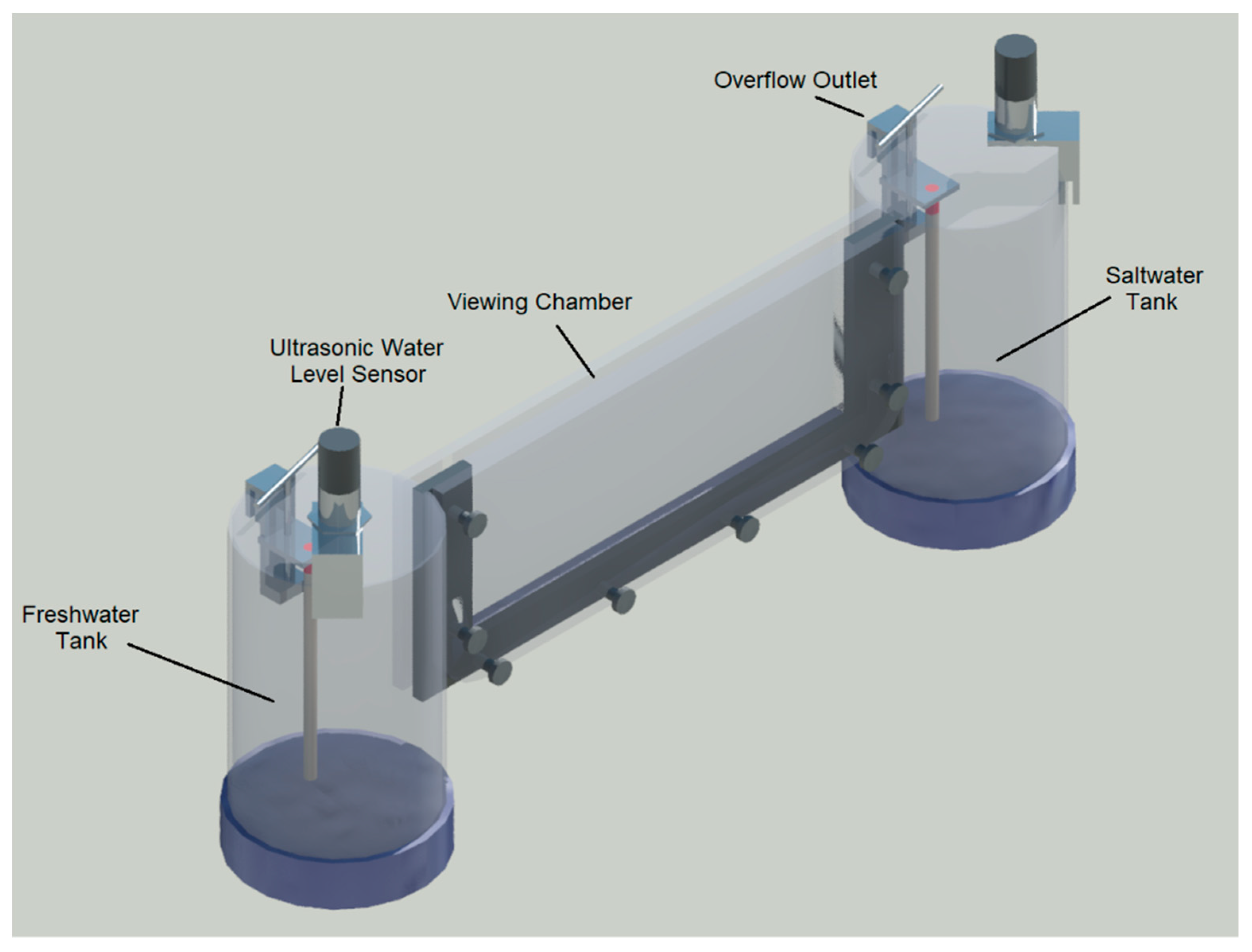
2. Laboratory Setup and Investigated Aquifers
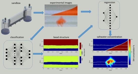
The sandbox apparatus depicted in Figure 1, described in detail by Robinson et al. [34], was used to investigate multiple scenarios of intrusion that allowed the generation of controlled and repeatable experimental data. It consists of a viewing chamber of dimensions 0.38 × 0.15 × 0.01 m with two cylindrical reservoir tanks on each side. The coastal aquifers were approximated by filling the central chamber with clear glass beads of predetermined diameters, supplied by Whitehouse Scientific®. In most test cases the reservoir on the left was filled with fresh water, while the one on the right contained saltwater with a density of 1025 kg/m3. The saltwater was dyed using red food colouring at a mix ratio of 0.15 g/L of solution. Two fine mesh acrylic screens were used to retain the beads in the main part of the apparatus while still permitting water circulation between the two tanks and the viewing chamber. Adjustable overflow outlets controlled the water level in the two side chambers and incremental changes in water level were achieved via the use of two Microsonic® (mic+25/DIU/TC, Microsonic GmbH, Dortmund, Germany) sensors. The measurements took place in a totally dark room. Lighting was introduced by two Camtree 600 LED light panels. A Nikon D850 Digital SLR Camera (D850 Digital SLR Camera, Nikon Corporation, Tokyo, Japan) equipped with a Nikkor FX 60 mm lens (Nikkor FX 60 mm, Nikon Corporation, Tokyo, Japan) was used to capture the experimental images. The 8-bit version of the images were used in the current investigation. The light panels were put on the back of the rig at a distance of 25 cm from the sandbox. The viewing chamber was positioned between the light source and the camera. The sandbox to camera distance was 95 cm. The domain area to be analysed was automatically derived from the rest of the image using the pre-processing algorithm introduced by Robinson et al. [34] using MATLAB R2018a (The MathWorks, Inc., Natick, MA, USA) application and programming language. The final cropped images had a resolution of 1185 × 3506 with a pixel size of 0.105 mm.
Beads of three different diameters, 780, 1090, and 1325 µm, were used in the current investigation. An intrinsic flow test on the experimental domain allowed calculation of the permeability of the porous media using Darcy’s law. Porosity was equal to 0.385, while permeability was equal to 7.98 × 10⁻¹⁰ m2, 1.83 × 10⁻⁹ m2, 2.39 × 10⁻⁹ m2, for the 780, 1090, and 1325 µm beads, respectively. In total, 15 aquifers were created (Table 1); four homogeneous aquifers for each utilized bead size and three heterogeneous ones. The heterogeneous cases, which are referred to as Layered1, Layered2 and Layered3, had three horizontal layers composed of distinct bead diameters (Figure 2). In Layered1, bead size increased in each heterogeneous layer from top to bottom, with 780 µm being the diameter in the upper layer, 1090 µm in the middle, and 1325 µm in the lower layer. In Layered2, the layout of the bead sizes was reversed such that 1325, 1090, and 780 µm were the sizes of the top, middle, and bottom layers, respectively. Layered3 had a low permeability layer, with a bead size of 780 µm, in the middle surrounded by two 1090 µm layers.
Two classical saltwater intrusion experiments, comparable to those introduced for the first time by Schincariol and Schwartz et al. [25] and Goswami1 and Clement [16], were recreated to develop and test the methodology employed. In the first, saltwater intrusion was initiated by hydraulic head difference between the freshwater and saltwater chambers ranging from 4 to 6 mm. This created a typical saltwater wedge in three homogeneous and the Layered1 and Layered2 heterogeneous aquifers (Figure 2a,b). In the second experiment, 10 mL of saltwater were injected into the upper part of the saturated freshwater only Layered3 aquifer. The saltwater plume was left to intrude deeper in the aquifer for five minutes. Subsequently flow was introduced by a 6 mm hydraulic head difference between the two tanks. Images were acquired each minute for 28 min, until the saline plume was completely flushed out of the aquifer (Figure 2c).

3. Methodology

The methodology introduced in this paper comprises three sections (Figure 3). The first part involves experimental image pre-processing via both established and novel procedures. The second part treats the task of recognizing aquifer heterogeneity as a multinomial pixel wise classification problem. Lastly the third section derives the saltwater concentration fields via regression analysis on the values of light intensity (LI) and the corresponding bead sizes. Artificial Neural Networks (ANN) were the learners favoured in this investigation, but the applicability of different machine learning algorithms was also established. Section 3.1, Section 3.2, Section 3.3 present the components of the subroutines in detail, including each of the steps followed by the authors in order to train the appropriate learners. Three homogeneous aquifers served as the training datasets for all the machine learning algorithms. The remaining aquifers were utilized for quantifying the models’ generalization ability (Table 1). It was established that all the training data necessary for the implementation of the method in heterogeneous aquifers with three different bead diameters, 780 µm, 1090 µm, and 1325 µm, could be generated by a single homogeneous aquifer per utilised bead size. After the training of the aforementioned learners was complete, saltwater concentration fields could be successfully generated with no further calibration effort for any number of new homogeneous or heterogeneous aquifers.

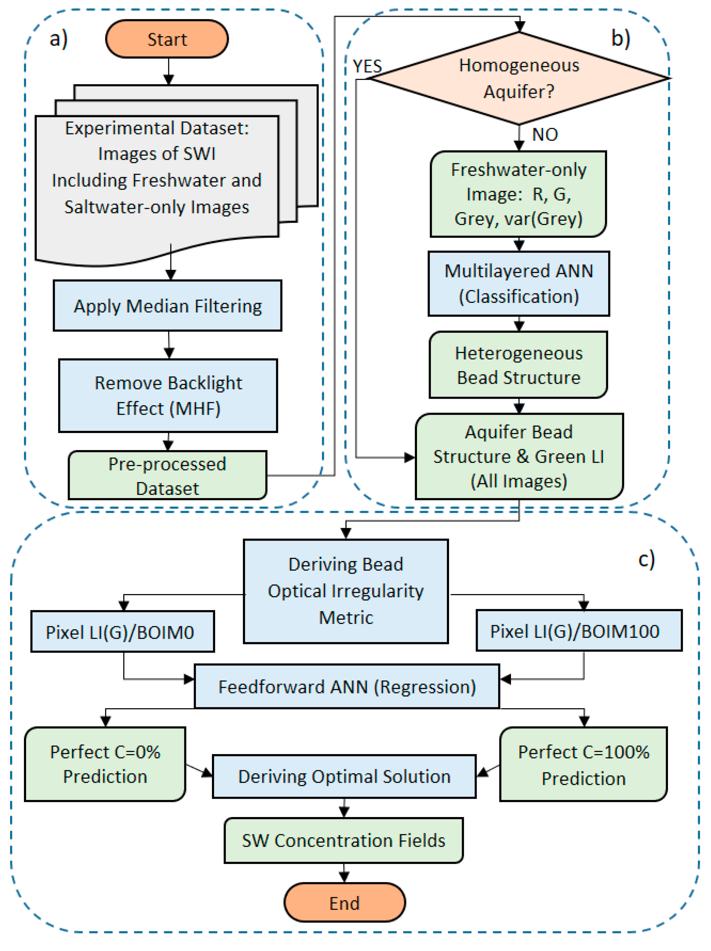
3.1. Image Pre-Processing

Data pre-processing significantly affects the generalization performance of supervised machine learning algorithms [55]. A 15 × 15 pixel median filter was applied to the acquired experimental data to diminish the impact of outliers. Despite this, the images of homogeneous aquifers were characterized by significant irregularity in the distribution of light intensity values. This can be attributed to two distinct factors: the different optical attributes of each specific glass bead and the lighting conditions. While the first cause creates a random variation in the observed LI values, the second is responsible for a distinct distribution, where the images appeared lighter in the centre of the sandbox. This lighting pattern was efficiently filtered out by developing the Mean Homogenization Factor (MHF) presented in Equation (1):
MHF ( x , y ) = 1 n × i = 1 n ( LI ( x , y , i ) / meanLI ( i ) )
where x, y are the pixel coordinates and n represents the three homogeneous aquifers, 780, 1090 and 1325 µm, used for neural training in the current investigation.
The mean value of light intensity for all colours in each of the aforementioned homogeneous images was calculated. Subsequently, the red (R), green (G), blue (B) and greyscale LI of every pixel was divided by the mean LI, giving the values of a Homogenization Factor for each pixel. By averaging the values of these factors for the three homogeneous aquifers, the effect of non-uniform backlighting was isolated from the random deviation caused by each individual bead. Dividing any given image with the values of MHF led to the successful normalization of its LI. The impact of the Mean Homogenization Factor on the LI distribution of the three training images is visualized in Figure 4. It is evident, that the application of MHF resulted in a starker LI distribution contrast between the three utilised bead sizes. This contributed to a significant improvement in the training and generalization performance of the machine learning algorithms tested in the next section.

3.2. Porous Medium Classification

A necessary step towards the elimination of aquifer-specific calibrations and to move beyond current pixel wise methodologies, is the ability to recognize the size of individual beads and thereby any given heterogeneous structure. Various classical and soft-computing approaches to image segmentation have been proposed over the years [56]. In the current paper a soft-computing method based on supervised machine learning is favoured. The proposed technique dissociates from image specific parameter configuration; based on qualitative evaluation of the investigated heterogeneous structures by the user, which is essential in classical methods, such as image thresholding or edge detection. This enables the automatic recognition of more complex, including totally random, experimental aquifers, while minimizing the time needed for recreating each one of them. This part of the investigation is based on images of the 15 aquifers taken prior to saltwater intrusion. The pixels of three homogeneous aquifers served as the training subset. The remaining twelve images were used to evaluate the effectiveness of the method. The training subset was deliberately kept as small as possible, in order to ensure the easy implementation of the approach.

3.2.1. Input Variable Selection

In machine learning applications, it has been demonstrated that successful variable selection can improve the prediction performance of the predictors while leading to faster and more cost-effective learners [57]. The three light intensity values (R, G, B) for each pixel, alongside their greyscale combination, were the basis of the input variable investigation. Moreover, it was established that the LI variance of the 15-by-15 neighbourhood around each input pixel provided an additional, useful feature for successfully distinguishing the three utilized bead sizes. This is because the larger bead diameters were associated with higher light intensity variance as depicted in Figure S1 of the supplementary material.
The relatively limited variable search space in the current problem, permitted the use of the more computationally intensive step-wise variable selection [58], instead of the much more commonly used, but less reliable, filter approaches. Artificial Neural Networks, with two hidden layers, consisting of 30 neurons each, were utilized for input variable selection. This ANN architecture was derived via trial and error. A sigmoid transfer function was used in the hidden neural layers and a softmax function [59] in the output layer, while Scaled Conjugate Gradient Backpropagation [60] served as the training algorithm. A network was trained for each one of the individual variables presented in Figure 5, to evaluate their fitness. The models were trained in parallel in a multi-core CPU, using MATLAB’s Neural Network Toolbox version 11.1 and Parallel Computing Toolbox version 6.12. The utilized subsets were randomly divided, such that 70% of the data was used for training, 15% for validation and 15% for testing. Early stopping was applied to prevent potential network overfitting [61]. The neural networks’ predictive ability was quantified by the percentage of successfully classified pixels on the 12 testing aquifers (Table 1).
The single variable which maximized model performance was the greyscale LI, thus it was chosen as the basis of the investigation. Subsequently, more variables were individually added to the training subset, and a new network was trained each time. As presented in Figure 5, the ANNs’ generalization ability on the heterogeneous aquifers was slightly lower than their performance on the homogeneous ones. This phenomenon was attributed to the distinct pattern in LI distribution observed in the heterogeneous cases due to the overlapping of layers of different bead sizes. The incorporation of blue LI, even though it improved the prediction of the homogeneous aquifers, caused an increase in pixel misclassification in the layered cases, particularly the 780 and 1090 µm ones, while 1325 µm beads were unaffected. The two smaller sizes, being predominantly blue (Figure 4), were prone to higher fluctuations of the values of B that negatively affected the network’s generalization performance; thus, any incorporation of blue LI or blue related variables was rejected. Through neural training, using nine different variable combinations, it was established that R, G, greyscale LI, and grayscale variance was the optimum training subset (Case 4 in Figure 5).

3.2.2. Evaluation of Various Machine Learning Algorithms

With the establishment of the optimum variable combination, the suitability of multiple machine learning techniques was investigated. MATLAB Statistics and Machine Learning Toolbox version 11.3 was utilized to train six well-known learners on 1185 × 3506 × 3 = 12.46 × 10⁶ data points, and their performance was compared with that of the neural network:
  • Linear Discriminant Analysis (LDA);
  • Quadratic Discriminant Analysis (QDA);
  • Fine and Medium k-nearest neighbours algorithms (KNN), with 1 and 10 neighbours, respectively;
  • 30-learner Boosted Tree Ensemble, using AdaBoost [62] ensemble learning algorithm;
  • 30-learner Random Forest [63].
All the MLT architectures were established via trial and error. The algorithms were trained in parallel and five-fold cross-validation was employed to prevent the learners from overfitting. Training times varied significantly between the seven MLTs (Table S1 of the Supplementary Material). In general, all the methods were able to predict bead structure of heterogeneous aquifers (Figure 6) with an accuracy of 98.85% or higher (Figure 7). It can be concluded that there was no need for stronger, more sophisticated learning algorithms or bigger training datasets. This indicates that the method proposed in the current paper can be easily adapted to different experimental setups in the future, utilizing various learners.

3.3. Generating Saltwater Concentration Fields

The image processing methods that have been presented up to now were based on the same principle [25,27,28,30,31]. A number of calibration images were acquired for each aquifer, these data were used to formulate a relationship between LI values and SW concentrations via regression analysis. While relatively accurate, these techniques were disadvantaged by the need to acquire new calibration images for every investigated aquifer, making them slow and labour intensive. Eliminating this need by the use of machine learning, will represent a step change in the ability to run significant laboratory investigations.
A traditional MLT approach would feed the raw data from the eight calibration images (with saltwater concentrations of 0%, 5%, 10%, 20%, 30%, 50%, 70%, and 100%), of one homogeneous aquifer for each utilized bead size, into a sufficiently strong learner that would automatically establish a relationship between LI and SW% [54]. Nevertheless, it is well documented [31,33] that experimental data of saltwater intrusion generated in sandbox setups are characterized by a high percentage of irregularity, mostly due to the deviating light absorbing attributes of the individual beads. The nature of this type of data makes their straightforward use for neural training problematic.
Instead of the actual images, a feedforward ANN with one 10-neuron hidden layer was trained on the mean values of monochromatic green LI for each specific aquifer (Figure 8) using Levenberg–Marquardt as its training algorithm [64]. This led to low training time and minimum training error (MSE~0.2 × 10⁻¹⁹), proving that the network’s size was sufficient. In 8-bit digital images, light intensities are expressed with 256 values, varying between 0 and 255. It was observed that in the pure saltwater images, the blue LI component values were minimized getting values close or equal to 0, while for many pixels red LI was equal to 255; thus, monochromatic green was favoured for SW concentration calculation [35].
In order to minimize the impact of noisy data, caused by the presence of beads of varying colour tones, a quantification of the optical irregularities of the glass bead medium was essential. This procedure took place in the freshwater-only images of the tested aquifers. To do so, the LI values of each individual pixel were divided with the corresponding measured average LI value of its bead size. In doing so, a Bead Optical Irregularity Metric (BOIM) was derived, characterising each specific bead of the investigated aquifers, as shown in Equation (2), assigning higher and lower BOIM values to lighter and darker beads, respectively.
BOIM ( x , y ) = LI ( x , y ) meanLI
where “meanLI” is specific to the local pixel bead size.
By dividing the freshwater only image of any aquifer with its corresponding BOIM matrix, the mean LI values the feedforward ANN was trained upon are returned. When these values were fed on the neural network, the 0% SW concentration fields was perfectly recreated. The same procedure was repeated for saltwater-only images of the aquifers, deriving the BOIM corresponding to the 100% saltwater percentage. This led to the perfect prediction of the 100% SW concentration components of the testing images. The two derived components of bead irregularity were not identical to each other in any of the investigated cases, proving that the level of light absorbance was not only correlated to the composition of each specific bead, but also to the dye concentration present. Thus, the distinction between the bead optical irregularity metric at C = 0% (BOIM0) and C = 100% (BOIM100) was deemed necessary.
Intruding saltwater wedge images are dominated by two distinct regions: the saltwater wedge, with 100% SW concentration; the pure freshwater part of the aquifer, where the intrusion has not occurred. The mixing zone makes up no more than 5% of the acquired data. Dividing the SWI test images with BOIM0 and BOIM100 creates two data subsets that, when fed to the neural network, generate a perfect prediction of the two main concentration regions. The effect of the implementation of the two factors on a test image is depicted in Figure 9.

3.4. Optimum Combination of Predicted Saltwater Concentration Fields

A crucial step towards the correct representation of the mixing zone on the salt-freshwater interface was the proper combination of values of the two, BOIM0 and BOIM100-modified, SW concentration fields. Figure 10 illustrates the mean squared error (MSE) generated by the ANN for the actual data of the homogeneous calibration images, expressing the difference between the calculated and the real SW%. For concentrations closer to 0%, the BOIM0-modified subsets generate less MSE. The same applies to the BOIM100-modified figures for bigger SW concentrations. A prediction combination based on this error distribution was formulated. For extremely small or big saltwater concentrations only the BOIM0 (zone 1) and the BOIM100 (zone 5) predictions were taken into account. In between zones 1 and 5, three distinct zones were favoured, where either simple (zone 3) or weighted averaging (zones 2 and 4) between the two predictions took place. A genetic algorithm, presented in detail in Appendix A, was utilised to optimize the limits of the five aforementioned concentration areas in order to minimize the generated MSE (Equation (A1)). The algorithm was executed eight times (Table A1) to derive an optimum solution. According to this solution, the best prediction combination was as follows: zone 1 = 0%–16%, zone 2 = 16%–33%, zone 3 = 33%–51%, zone 4 = 51%–88% and zone 5 = 88%–100% (Figure 10). Since prediction error depends on the optical characteristics of the glass bead medium, dye and back lighting (factors which remain consistent), the prediction combination needs to be optimized only once for each experimental setup.
The presented procedure took advantage of the capabilities of supervised machine learning. It turned a highly noisy experimental dataset, in which relatively strong learners failed to predict its concentration values, into two subsets by filtering out much of the noise introduced by the variance in light absorbing attributes of individual glass beads. The two subsets were then fed into a less complex neural network. By properly combining the two predictions, high quality saltwater concentration fields were obtained.

4. Results

Saltwater concentration fields generated using the novel machine learning based method presented in this paper and concentration fields derived from the pixel wise regression method introduced by Robinson et al. [34] were compared with each other. For the first experimental case, steady state images of SWI, introduced by a hydraulic head difference equal to 6 mm, in the three homogeneous aquifers (780, 1090, and 1325 µm) and Layered1, Layered2 heterogeneous aquifers were processed using the two methodologies (Figure 11a–e). To further investigate the ability of the new procedure to recreate quality concentration fields of heterogeneous aquifers, and to quantify any performance difference between steady and unsteady state conditions, two additional cases were investigated. The images of the layered aquifers were acquired exactly 20 min after the difference of hydraulic head between the freshwater and saltwater chamber was reduced from 6 to 4 mm and while the intruding SW wedge had not yet stabilized (Figure 11f,g). In the second experimental case, the actual test figures of moving saltwater plume are presented alongside the corresponding generated flow fields two, five, nine and fifteen minutes after the injection of saltwater in the Layered3 heterogeneous aquifer (Figure 12).
Recognizing any significant difference between the SW concentration fields generated by the two methods through simple visual observation (Figure 11 and Figure S2 of the Supplementary Material) was not feasible for the majority of the test cases. During the data acquisition procedure, air bubbles were formed in the upper part of the homogeneous 1090 and 1325 µm aquifers. This is an experimental error reported before by Robinson et al. [34], that can only be avoided through the use of degassed water, further complicating the laboratory procedure. Even though bubbles appeared as spots of over-predicted SW concentration in the pixel wise calculated concentration maps (Figure 11b(i),c(i)), they did not affect the maps generated with the novel technique (Figure 11b(ii),c(ii)) that recreated the freshwater only parts of the images successfully. This makes the use of regular tap water compatible with the presented image analysis procedure.
Three variables were utilized to quantify the difference between the results of the two procedures; the toe length (TL) of the intruding wedge, the width of the mixing zone (WMZ) and the average difference between the concentration values generated by the two procedures (ΔC) (Figure 13). TL was defined as the maximum horizontal distance of the 50% concentration isoline from the right aquifer edge, while WMZ equalled the average vertical distance between the 25% and 75% concentration isolines.
The maximum TL difference between the two methods was observed in the steady state case of the Layered2 heterogeneous aquifer. It was less than 0.6 mm, or 6 pixels, which correspond to between 45% and 76% of a single glass bead diameter. The prediction of the width of the mixing zone was extremely similar for the two methods, giving a difference of 0.01 mm~0.23 mm. Average ΔC across most testing images was less than 2%, with the exception of the Layered2 steady state case. No distinct difference was observed in the performance of the new method between the homogenous and heterogeneous aquifers, steady and unsteady state cases, or the wedge shaped and saline plume intrusion data. This demonstrates the method’s resilience, indicating it can be applied to a diverse set of laboratory investigations.

5. Conclusions

This paper presents a novel method of incorporating machine learning techniques in laboratory investigations of saltwater intrusion in coastal aquifers. The procedure consists of three distinct parts. Initially an approach of filtering out back lighting noise was presented. The second section included the training of a learner to conduct pixel-wise bead size classification analysis that automatically recreated the ground stratification of the investigated laboratory aquifers. In the third part, the generated bead size was used alongside the acquired values of monochromatic green light intensity to train an Artificial Neural Network in correlating LI values with saltwater concentrations (regression analysis). A procedure for quantifying the optical irregularity of individual glass beads was proposed. This enabled the minimization of the irregularity’s impact on the generalization performance of the regression ANN, leading to highly accurate SW concentration fields.
The main advantage of the methodology is the minimization of aquifer-specific calibrations, thus significantly lowering the time needed for experimental data acquisition. Instead of obtaining calibration images for every tested aquifer, they are obtained only once at the initial stage of the investigation and are used for neural training. Apart from the freshwater and saltwater only images, any subsequent acquisition of calibration data, for any new aquifers, is deemed redundant. In the utilized apparatus, this leads to time savings of up to five hours of labour-intensive laboratory work per tested case. This advantage becomes crucial for larger-scale investigations that would include multiple heterogeneous aquifers with potentially larger sandbox dimensions. In conclusion, the machine learning oriented technique gave satisfactory results for homogeneous and heterogeneous aquifers alike. The proposed methodology presented a series of additional advantages over prior methods.
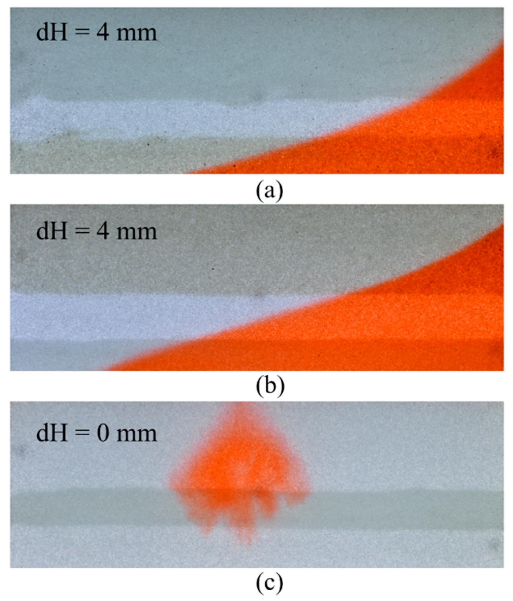
  • The method outperformed pixel-wise regression in most cases. It perfectly recreated the pure freshwater and saltwater zones of the experimental SW intrusion data. The impact of air bubbles was limited. Since the regression was not performed on a pixel wise level, there was no need for perfect overlap between the test and calibration images, thus small movements of the camera introduced minimal error.
  • The approach was implemented successfully for the wedge-shaped intrusion and the irregularly shaped saltwater plume alike, proving its resilience and applicability on diverse setups of saline intrusion. The basic principles of the methodology may be extensible to laboratory investigations of phenomena beyond this specific research field, such as contaminant transport of dense or non-aqueous phase liquids.
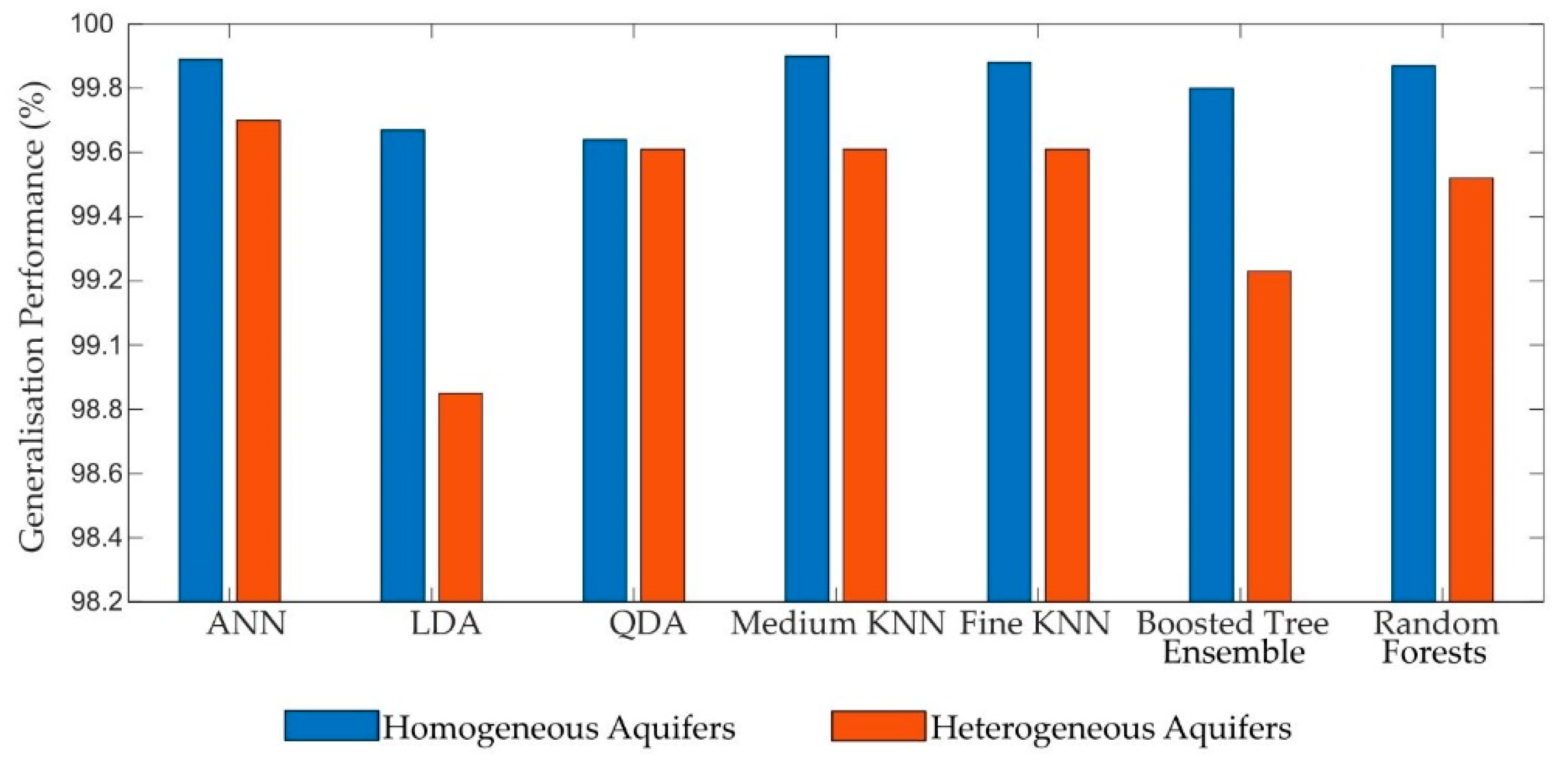
  • The results confirmed that a minimum of one homogeneous aquifer per utilized bead size generated sufficient training data for the implementation of the method. It was established that the procedure can be recreated by substituting the ANNs with different machine learning algorithms. All the algorithms used were well established and their architecture was derived through trial and error. The application of more complex learning procedures, such as deep learning, was not necessary. The aforementioned facts demonstrate that the method’s implementation is straightforward and does not require advanced machine learning skills, making it a user friendly scientific tool.

Supplementary Materials

The following are available online at https://0-www-mdpi-com.brum.beds.ac.uk/2073-4441/12/11/2996/s1, Figure S1: Grayscale light intensity variance of 15-by-15 pixel neighborhood in the (a) 780 µm, (b) 1090 µm, and (c) 1325 µm homogeneous aquifers, Figure S2: Saltwater concentration fields generated by (i) pixel wise regression (left) and (ii) the proposed ML technique (right), (a) two (b) five (c) nine and (d) fifteen minutes after the injection of saltwater in Layered3 heterogeneous aquifer, Table S1: Training time of the investigated machine learning techniques.

Author Contributions

Conceptualization, G.E. and G.A.H.; methodology, G.E.; software, G.E. and E.M.B.; validation, G.E. and G.A.H.; formal analysis, G.E.; investigation, G.E.; resources, J.F.Á. and M.C.M; data curation, G.E.; writing—original draft preparation, G.E.; writing—review and editing, G.H., E.M.B., J.F.Á., M.C.M., R.F. and A.A.A.; visualization, G.E. and E.M.B.; supervision, G.A.H. and R.F.; project administration, G.A.H.; funding acquisition, G.A.H. All authors have read and agreed to the published version of the manuscript.

Funding

This work was funded by EPSRC Standard Research (Grant No. EP/R019258/1).

Acknowledgments

The authors would like to thank Desmond Hill for support with the laboratory apparatus and Jonathon Campbell for assistance with the data acquisition. The relevant data arising from this research are listed in the tables, and figures contained herein. Any additional details may be obtained from the corresponding author ([email protected]).

Conflicts of Interest

The authors declare no conflict of interest.

Appendix A. Deriving the Optimum Combination of Predicted Saltwater Concentrations

The combination of the two saltwater concentration predictions generated using the BOIM0 and BOIM100 subsets was based on the five distinct zones described in Section 3.3. A genetic algorithm was utilized to optimize the boundaries of these sections. Genetic algorithms are nature-inspired heuristic optimization procedures that minimize a specific relationship called the objective function. In the current case it was the MSE of the generated saltwater concentration fields. The calculation of the mean squared error was based on the 24 calibration images of the three homogeneous aquifers. The algorithm’s objective function included five variables, representing the width of each zone (x1, x2, x3, x4, x5). Since calibration concentrations were skewed towards 0%, using the total MSE generated for the aforementioned images as the algorithm’s objective function, would constitute an underestimation of the error in bigger concentrations. A weighted averaging of the MSE between every two consecutive calibration images (Figure A1) was used instead for each one of the three aquifers (Equation (A1)):
O b j . F u n c t i o n ( x 1 ,   x 5 ) = j = 1 3 ( i = 1 7 ( w e i g h t ( i , j ) × M S E ( i , j ) , M S E ( i + 1 , j ) ¯ ) ) / 3  
where j is the number of homogeneous aquifers (three) and i is the number of calibration concentrations (eight). An initial solution population of 500 was deemed sufficient, while the genetic procedures were implemented for 100 generations. The algorithm was executed for a total of eight times (Table A1) to derive the optimum solution.
Figure A1. Calculation of weights for the weighted averaging of generated Mean Squared Error.
Water 12 02996 g0a1
Table A1. Results of the eight executions of the Genetic Algorithm. The optimum solution was generated in Run 3.
RunErrorx1x2x3x4x5
15.894651616213611
25.99991812203317
35.83231617183712
46.14206203293414
55.868117730433
66.3134121228408
75.93311813193614
85.99247181022419

References

  1. Neumann, B.; Vafeidis, A.T.; Zimmermann, J.; Nicholls, R.J. Future Coastal Population Growth and Exposure to Sea-Level Rise and Coastal Flooding—A Global Assessment. PLoS ONE 2015, 10, e0118571. [Google Scholar] [CrossRef] [PubMed]
  2. Voss, C.; Souza, W.R. Variable Density Flow and Solute Transport Simulation of Regional Aquifers Containing a Narrow Freshwater-Saltwater Transition Zone. Water Resour. Res. 1987, 23, 1851–1866. [Google Scholar] [CrossRef]
  3. Bear, J. Dynamics of Fluids in Porous Media; American Elsevier Publishing Company: New York, NY, USA, 1988. [Google Scholar]
  4. Herbert, A.W.; Jackson, C.P.; Lever, D.A. Coupled Groundwater Flow and Solute Transport with Fluid Density Strongly Dependent Upon Concentration. Water Resour. Res. 1988, 24, 1781–1795. [Google Scholar] [CrossRef]
  5. Stoeckl, L.; Houben, G.J.; Dose, E.J. Experiments and Modeling of Flow Processes in Freshwater Lenses in Layered Island Aquifers: Analysis of Age Stratification, Travel Times and Interface Propagation. J. Hydrol. 2015, 529, 159–168. [Google Scholar] [CrossRef]
  6. Strack, O.D.L.; Stoeckl, L.; Damm, K.; Houben, G.; Ausk, B.K.; de Lange, W.J. Reduction of Saltwater Intrusion by Modifying Hydraulic Conductivity. Water Resour. Res. 2016, 52, 6978–6988. [Google Scholar] [CrossRef] [Green Version]
  7. Werner, A.D.; Kawachi, A.; Laattoe, T. Plausibility of Freshwater Lenses Adjacent to Gaining Rivers: Validation by Laboratory Experimentation. Water Resour. Res. 2016, 52, 8487–8499. [Google Scholar] [CrossRef]
  8. Noorabadi, S.; Nazemi, A.H.; Sadraddini, A.A.; Delirhasannia, R. Laboratory Investigation of Water Extraction Effects on Saltwater Wedge Displacement. Glob. J. Environ. Sci. Manag. 2017, 1, 21–32. [Google Scholar]
  9. Noorabadi, S.; Sadraddini, A.A.; Nazemi, A.H.; Delirhasannia, R. Laboratory and Numerical Investigation of Saltwater Intrusion into Aquifers. J. Mater. Environ. Sci. 2017, 8, 4273–4283. [Google Scholar] [CrossRef]
  10. Luyun, R.; Momii, K.; Nakagawa, K. Effects of Recharge Wells and Flow Barriers on Seawater Intrusion. Groundwater 2011, 49, 239–249. [Google Scholar] [CrossRef]
  11. Abdelgawad, A.M.; Abdoulhalik, A.; Ahmed, A.A.; Moutari, S.; Hamill, G. Transient Investigation of the Critical Abstraction Rates in Coastal Aquifers: Numerical and Experimental Study. Water Resour. Manag. 2018, 32, 3563–3577. [Google Scholar] [CrossRef] [Green Version]
  12. Takahashi, M.; Momii, K.; Luyun, R. Laboratory Scale Investigation of Dispersion Effects on Saltwater Movement Due to Cutoff Wall Installation. E3S Web Conf. 2018, 54, 6. [Google Scholar] [CrossRef]
  13. Abdoulhalik, A.; Ahmed, A.A. Transience of Seawater Intrusion and Retreat in Response to Incremental Water-Level Variations. Hydrol. Process. 2018, 32, 2721–2733. [Google Scholar] [CrossRef]
  14. Liu, Y.; Mao, X.; Chen, J.; Barry, D.A. Influence of a Coarse Interlayer on Seawater Intrusion and Contaminant Migration in Coastal Aquifers. Hydrol. Process. 2014, 28, 5162–5175. [Google Scholar] [CrossRef]
  15. Shi, W.; Lu, C.; Ye, Y.; Wu, J.; Li, L.; Luo, J. Assessment of the Impact of Sea-Level Rise on Steady-State Seawater Intrusion in a Layered Coastal Aquifer. J. Hydrol. 2018, 563, 851–862. [Google Scholar] [CrossRef]
  16. Goswami, R.R.; Clement, T.P. Laboratory-Scale Investigation of Saltwater Intrusion Dynamics. Water Resour. Res. 2007, 43. [Google Scholar] [CrossRef]
  17. Mehdizadeh, S.S.; Werner, A.D.; Vafaie, F.; Badaruddin, S. Vertical Leakage in Sharp-Interface Seawater Intrusion Models of Layered Coastal Aquifers. J. Hydrol. 2014, 519, 1097–1107. [Google Scholar] [CrossRef]
  18. Stoeckl, L.; Houben, G. Flow Dynamics and Age Stratification of Freshwater Lenses: Experiments and Modeling. J. Hydrol. 2012, 458–459, 9–15. [Google Scholar]
  19. Dose, E.J.; Stoeckl, L.; Houben, G.J.; Vacher, H.L.; Vassolo, S.; Dietrich, J.; Himmelsbach, T. Experiments and Modeling of Freshwater Lenses in Layered Aquifers: Steady State Interface Geometry. J. Hydrol. 2014, 509, 621–630. [Google Scholar] [CrossRef]
  20. Houben, G.J.; Stoeckl, L.; Mariner, K.E.; Choudhury, A.S. The Influence of Heterogeneity on Coastal Groundwater Flow—Physical and Numerical Modeling of Fringing Reefs, Dykes and Structured Conductivity Fields. Adv. Water Resour. 2018, 113, 155–166. [Google Scholar] [CrossRef]
  21. Abarca, E.; Clement, T.P. A Novel Approach for Characterizing the Mixing Zone of a Saltwater Wedge. Geophys. Res. Lett. 2009, 36. [Google Scholar] [CrossRef] [Green Version]
  22. Lu, C.; Chen, Y.; Zhang, C.; Luo, J. Steady-State Freshwater-Seawater Mixing Zone in Stratified Coastal Aquifers. J. Hydrol. 2013, 505, 24–34. [Google Scholar] [CrossRef]
  23. Li, F.; Chen, X.; Liu, C.; Lian, Y.; He, L. Laboratory Tests and Numerical Simulations on the Impact of Subsurface Barriers to Saltwater Intrusion. Nat. Hazards 2018, 91, 1223–1235. [Google Scholar] [CrossRef]
  24. Armanuos, A.M.; Ibrahim, M.G.; Mahmod, W.E.; Takemura, J.; Yoshimura, C. Analysing the Combined Effect of Barrier Wall and Freshwater Injection Countermeasures on Controlling Saltwater Intrusion in Unconfined Coastal Aquifer Systems. Water Resour. Manag. 2019, 33, 1265–1280. [Google Scholar] [CrossRef]
  25. Schincariol, R.A.; Schwartz, F.W. An Experimental Investigation of Variable Density Flow and Mixing in Homogeneous and Heterogeneous Media. Water Resour. Res. 1990, 26, 2317–2329. [Google Scholar] [CrossRef]
  26. Zhang, Q.; Volker, R.E.; Lockington, D.A. Influence of Seaward Boundary Condition on Contaminant Transport in Unconfined Coastal Aquifers. J. Contam. Hydrol. 2001, 49, 201–215. [Google Scholar] [CrossRef]
  27. Zhang, Q.; Volker, R.E.; Lockington, D.A. Experimental Investigation of Contaminant Transport in Coastal Groundwater. Adv. Environ. Res. 2002, 6, 229–237. [Google Scholar] [CrossRef]
  28. Konz, M.; Ackerer, P.; Meier, E.; Huggenberger, P.; Zechner, E.; Gechter, D. On the Measurement of Solute Concentrations in 2-D Flow Tank Experiments. Hydrol. Earth Syst. Sci. 2008, 12, 727–738. [Google Scholar] [CrossRef] [Green Version]
  29. Konz, M.; Younes, A.; Ackerer, P.; Fahs, M.; Huggenberger, P.; Zechner, E. Variable-Density Flow in Heterogeneous Porous Media—Laboratory Experiments and Numerical Simulations. J. Contam. Hydrol. 2009, 108, 168–175. [Google Scholar] [CrossRef]
  30. Konz, M.; Ackerer, P.; Younes, A.; Huggenberger, P.; Zechner, E. Two-Dimensional Stable-Layered Laboratory-Scale Experiments for Testing Density-Coupled Flow Models. Water Resour. Res. 2009, 45, 2. [Google Scholar] [CrossRef] [Green Version]
  31. Liu, S.; Tao, A.; Dai, C.; Tan, B.; Shen, H.; Zhong, G.; Lou, S.; Chalov, S.; Chalov, R. Experimental Study of Tidal Effects on Coastal Groundwater and Pollutant Migration. Water Air Soil Pollut. 2017, 228, 163. [Google Scholar] [CrossRef]
  32. Kuan, W.K.; Jin, G.; Xin, P.; Robinson, C.; Gibbes, B.; Li, L. Tidal Influence on Seawater Intrusion in Unconfined Coastal Aquifers. Water Resour. Res. 2012, 48. [Google Scholar] [CrossRef] [Green Version]
  33. Konz, M.; Ackerer, P.; Huggenberger, P.; Veit, C. Comparison of Light Transmission and Reflection Techniques to Determine Concentrations in Flow Tank Experiments. Exp. Fluids 2009, 47, 85–93. [Google Scholar] [CrossRef] [Green Version]
  34. Robinson, G.; Hamill, G.A.; Ahmed, A.A. Automated Image Analysis for Experimental Investigations of Salt Water Intrusion in Coastal Aquifers. J. Hydrol. 2015, 530, 350–360. [Google Scholar] [CrossRef] [Green Version]
  35. Etsias, G.; Hamill, G.; Benner, E.; Aguila, J.F.; Mc Donnell, M.; Flynn, R. The effect of colour depth and image resolution on laboratory scale study of aquifer saltwater intrusion. In CERAI 2020; Civil Enigineering Association Ireland, Ed.; Civil Engineering Association Ireland: Cork, Ireland, 2020. [Google Scholar]
  36. Robinson, G.; Ahmed, A.A.; Hamill, G.A. Experimental Saltwater Intrusion in Coastal Aquifers Using Automated Image Analysis: Applications to Homogeneous Aquifers. J. Hydrol. 2016, 538, 304–313. [Google Scholar] [CrossRef] [Green Version]
  37. Abdoulhalik, A.; Ahmed, A.A.; Hamill, G.A. A New Physical Barrier System for Seawater Intrusion Control. J. Hydrol. 2017, 549, 416–427. [Google Scholar] [CrossRef] [Green Version]
  38. Abdoulhalik, A.; Ahmed, A.A. The Effectiveness of Cutoff Walls to Control Saltwater Intrusion in Multi-Layered Coastal Aquifers: Experimental and Numerical Study. J. Environ. Manag. 2017, 199, 62–73. [Google Scholar] [CrossRef] [Green Version]
  39. Abdoulhalik, A.; Ahmed, A.A. How Does Layered Heterogeneity Affect the Ability of Subsurface Dams to Clean up Coastal Aquifers Contaminated with Seawater Intrusion? J. Hydrol. 2017, 553, 708–721. [Google Scholar] [CrossRef] [Green Version]
  40. Wipfler, E.L.; Ness, M.; Breedveld, G.D.; Marsman, A.; van der Zee, S.E.A.T.M. Infiltration and Redistribution of Lnapl into Unsaturated Layered Porous Media. J. Contam. Hydrol. 2004, 71, 47–66. [Google Scholar] [CrossRef]
  41. Oostrom, M.; Hofstee, C.; Wietsma, T.W. Behavior of a Viscous Lnapl under Variable Water Table Conditions. Soil Sediment Contam. Int. J. 2006, 15, 543–564. [Google Scholar] [CrossRef]
  42. O’Carroll, D.M.; Sleep, B.E. Hot Water Flushing for Immiscible Displacement of a Viscous Napl. J. Contam. Hydrol. 2007, 91, 247–266. [Google Scholar] [CrossRef]
  43. Sun, S. Transient Water Table Influence Upon Light Non-Aqueous Phase Liquids (Lnapls) Redistribution: Laboratory and Modelling Studies; University of Birmingham: Birmingham, UK, 2016. [Google Scholar]
  44. Gramling, C.; Harvey, C.F.; Meigs, L.C. Reactive Transport in Porous Media:  A Comparison of Model Prediction with Laboratory Visualization. Environ. Sci. Technol. 2002, 36, 2508–2514. [Google Scholar] [CrossRef] [PubMed]
  45. Katz, G.E.; Berkowitz, B.; Guadagnini, A.; Saaltink, M.W. Experimental and Modeling Investigation of Multicomponent Reactive Transport in Porous Media. J. Contam. Hydrol. 2011, 120–121, 27–44. [Google Scholar] [PubMed]
  46. Castro-Alcalá, E.; Fernàndez-Garcia, D.; Carrera, J.; Bolster, D. Visualization of Mixing Processes in a Heterogeneous Sand Box Aquifer. Environ. Sci. Technol. 2012, 46, 3228–3235. [Google Scholar] [CrossRef] [PubMed]
  47. Poonoosamy, J.; Kosakowski, G.; Van Loon, L.R.; Mäder, U. Dissolution–Precipitation Processes in Tank Experiments for Testing Numerical Models for Reactive Transport Calculations: Experiments and Modelling. J. Contam. Hydrol. 2015, 177–178, 1–17. [Google Scholar] [CrossRef] [PubMed]
  48. Dausman, A.M.; Langevin, C.D. Movement of the saltwater interface in the surficial aquifer system in response to hydrologic stresses and water-management practices, broward county, Florida. In Scientific Investigations Report; U.S. Geological Survey, Information Services: Denver, CO, USA, 2005. [Google Scholar]
  49. Yoon, H.; Kim, Y.; Ha, K.; Lee, S.; Kim, G. Comparative Evaluation of Ann- and Svm-Time Series Models for Predicting Freshwater-Saltwater Interface Fluctuations. Water 2017, 9, 323. [Google Scholar] [CrossRef] [Green Version]
  50. Lal, A.; Datta, B. Development and Implementation of Support Vector Machine Regression Surrogate Models for Predicting Groundwater Pumping-Induced Saltwater Intrusion into Coastal Aquifers. Water Resour. Manag. 2018, 32, 2405–2419. [Google Scholar] [CrossRef]
  51. Lal, A.; Datta, B. Modelling Saltwater Intrusion Processes and Development of a Multi-Objective Strategy for Management of Coastal Aquifers Utilizing Planned Artificial Freshwater Recharge. Modeling Earth Syst. Environ. 2018, 4, 111–126. [Google Scholar] [CrossRef]
  52. Roy, D.; Datta, B. A Review of Surrogate Models and Their Ensembles to Develop Saltwater Intrusion Management Strategies in Coastal Aquifers. Earth Syst. Environ. 2018, 2, 193–211. [Google Scholar] [CrossRef]
  53. Lal, A.; Datta, B. Multi-Objective Groundwater Management Strategy under Uncertainties for Sustainable Control of Saltwater Intrusion: Solution for an Island Country in the South Pacific. J. Environ. Manag. 2019, 234, 115–130. [Google Scholar] [CrossRef]
  54. Robinson, G.; Moutari, S.; Ahmed, A.A.; Hamill, G.A. An Advanced Calibration Method for Image Analysis in Laboratory-Scale Seawater Intrusion Problems. Water Resour. Manag. 2018, 32, 3087–3102. [Google Scholar] [CrossRef] [Green Version]
  55. Kotsiantis, S.B.; Kanellopoulos, D.; Pintelas, P.E. Data Preprocessing for Supervised Leaning. Int. J. Comput. Sci. 2006, 1, 111–117. [Google Scholar]
  56. De, S.; Bhattacharyya, S.; Chakraborty, S.; Dutta, P. Computational intelligence methods and applications. In Hybrid Soft Computing for Multilevel Image and Data Segmentation; Springer International Publishing: Basel, Switzerland, 2018. [Google Scholar]
  57. Guyon, I.; Elisseeff, A. An Introduction to Variable and Feature Selection. J. Mach. Learn. Res. 2003, 3, 1157–1182. [Google Scholar]
  58. May, R.; Dandy, G.; Maier, H. Review of input variable selection methods for artificial neural networks. In Artificial Neural Networks—Methodological Advances and Biomedical Applications; InTechOpen: London, UK, 2011. [Google Scholar]
  59. Bishop, C.M. Pattern Recognition and Machine Learning; Springer: New York, NY, USA, 2006. [Google Scholar]
  60. Møller, M.F. A Scaled Conjugate Gradient Algorithm for Fast Supervised Learning. Neural Netw. 1993, 6, 525–533. [Google Scholar] [CrossRef]
  61. Bishop, C.M. Neural Networks for Pattern Recognition; Oxford University Press, Inc.: Hong Kong, 1995. [Google Scholar]
  62. Freund, Y.; Schapire, R.E. A Decision-Theoretic Generalization of on-Line Learning and an Application to Boosting. J. Comput. System Sci. 1997, 55, 119–139. [Google Scholar] [CrossRef] [Green Version]
  63. Breiman, L. Random Forests. Mach. Learn. 2001, 45, 5–32. [Google Scholar] [CrossRef] [Green Version]
  64. Hagan, M.T.; Menhaj, M.B. Training Feedforward Networks with the Marquardt Algorithm. IEEE Trans. Neural Netw. 1994, 5, 989–993. [Google Scholar] [CrossRef] [PubMed]
Figure 1. Three-dimensional representation of the sandbox tank.
Water 12 02996 g001
Figure 2. Photos of laboratory-induced saline intrusion in the three stratified aquifers. Experiment 1: saline wedge intruding into (a) Layered1 and (b) Layered2 aquifers, 20 min after the hydraulic head difference was changed from 6 to 4 mm. Experiment 2: the saline plume, 3 min after its introduction to the (c) Layered3 aquifer, while no head difference is applied between the left and right side tanks.
Water 12 02996 g002
Figure 3. Flowchart of the proposed methodology depicting its three distinct parts (a) image pre-processing, (b) bead structure recognition and (c) saltwater field generation.
Water 12 02996 g003
Figure 4. Light intensity distribution of the (a) original and (b) homogenized training images.
Water 12 02996 g004
Figure 5. Percentage of misclassified pixels of homogeneous and heterogeneous aquifers by the pattern recognition ANNs trained on the nine different input variable subsets.
Water 12 02996 g005
Figure 6. Heterogeneous aquifers (i) (a) Layered1, (b) Layered2, (c) Layered3 and (ii) bead structure generated by a multi-layered Artificial Neural Network (ANN).
Water 12 02996 g006
Figure 7. Generalization Performance of seven distinct machine learning techniques (MLT).
Water 12 02996 g007
Figure 8. Average values of green light intensity of the three homogeneous aquifers for each corresponding calibration concentration.
Water 12 02996 g008
Figure 9. Effect of the implementation of BOIM0 and BOIM100 on a SWI image of the Layered2 aquifer.
Water 12 02996 g009
Figure 10. MSE generated by the BOIM0 and BOIM100 modified subsets for the three homogeneous aquifers and the proposed optimum combination of the predictions.
Water 12 02996 g010
Figure 11. Steady state saltwater concentration fields of the (a) 780 µm, (b) 1090 µm, and (c) 1325 µm, homogeneous, and the (d) Layered1 and (e) Layered2 heterogeneous aquifers. Transient state SW concentration fields of the (f) Layered1 and (g) Layered2 heterogeneous aquifers generated by (i) pixel wise regression (left) and by (ii) the proposed ML technique (right).
Water 12 02996 g011
Figure 12. Experimental images (i) and saltwater concentration fields (ii) generated by the proposed ML technique (a) two (b) five (c) nine and (d) fifteen minutes after the injection of saltwater in the Layered3 heterogeneous aquifer.
Water 12 02996 g012
Figure 13. Absolute difference between the (a) toe length (TL), (b) width of mixing zone (WMZ) and (c) average difference of saltwater concentrations (ΔC) derived by the two methods for the eleven investigated test images.
Water 12 02996 g013
Table 1. Experimental aquifer images used as training and testing datasets by the classification and regression machine learning algorithms.
Bead Structure Recognition (Classification)
Training ImagesTesting Images
Freshwater-only ImagesFreshwater-only Images
Total Number of Images: 3Total Number of Images: 12
1 Homogeneous 780 μm3 Homogeneous 780 μm
1 Homogeneous 1090 μm3 Homogeneous 1090 μm
1 Homogeneous 1325 μm3 Homogeneous 1325 μm
3 Layered Aquifers
SW Concentration Field Generation (Regression)
Training ImagesTesting Images
(0%, 5%, 10%, 20%, 30%, 50% Head Driven SWI and
70%,100% Concentration Images)SW Plume Flow Images
Total Number of Images: 24Total Number of Images: 11
1 Homogeneous 780 μm (8 Images)1 Homogeneous 780 μm
1 Homogeneous 1090 μm (8 Images)1 Homogeneous 1090 μm
1 Homogeneous 1325 μm (8 Images)1 Homogeneous 1325 μm
3 Layered Aquifers (8 Images)
Publisher’s Note: MDPI stays neutral with regard to jurisdictional claims in published maps and institutional affiliations.

