Experimental Research and Numerical Analysis of Flow Phenomena in Discharge Object with Siphon


1
Centre of Hydraulic Research, Jana Sigmunda 313, 78349 Lutín, Czech Republic
2
Institute of Thermomechanics, Czech Academy of Sciences, Dolejškova 1402/5, 18200 Praha 8, Czech Republic
3
Faculty of Mechanical Engineering, University of West Bohemia in Pilsen, Univerzitní 8, 30614 Plzeň, Czech Republic
*
Author to whom correspondence should be addressed.
Water 2020, 12(12), 3330; https://0-doi-org.brum.beds.ac.uk/10.3390/w12123330
Submission received: 22 October 2020
/
Revised: 17 November 2020
/
Accepted: 23 November 2020
/
Published: 27 November 2020
(This article belongs to the Section Hydraulics and Hydrodynamics)
Abstract
:This article presents results of the experimental research and numerical simulations of the flow in a pumping system’s discharge object with the welded siphon. The laboratory simplified model was used in the study. Two stationary flow regimes characterized by different volume flow rates and water level heights have been chosen. The study concentrates mainly on the regions below and behind the siphon outlet. The mathematical modelling using advanced turbulence models has been performed. The free-surface flow has been carried out by means of the volume-of-fluid method. The experimental results obtained by the particle image velocimetry method have been used for the mathematical model validation. The evolution and interactions of main flow structures are analyzed using visualizations and the spectral analysis. The presented results show a good agreement of the measured and calculated complex flow topology and give a deep insight into the flow structures below and behind the siphon outlet. The presented methodology and results can increase the applicability and reliability of the numerical tools used for the design of the pump and turbine stations and their optimization with respect to the efficiency, lifetime and environmental demands.
1. Introduction
This paper presents one part of the results of the project, focused on the improvement and verification of numerical tools, used for an optimal design of pumping stations. The pumping station is a complete hydraulic system, consisting typically of one or several pumps, the intake and discharge objects and the necessary connecting piping. This paper concentrates on the numerical modelling of flow in the discharge objects with siphons and its validation by the experimental results obtained using camera-based visualizations and the particle image velocimetry (hereinafter, PIV) measuring technique.
The pumping stations widely use the discharge objects with the siphons, as they are easy-to-install and easy-to-operate and require minimum mechanical components. The flow in these output hydro-machine objects could be characterized by specific features. It is typically a combination of the diffuser flow and the free jet flow which interacts with still fluid and impinges on a wall. Typically, the fluid is a two-phase one with both the liquid and gas fractions. Until now, there is no systematic study of this specific case in the literature. Overall, the case represents a tough problem both from the point of view of the physical modelling using the experimental research and mathematical simulations involving the so-called computational fluid dynamics (hereinafter CFD). Our paper represents a contribution to fill this gap.
Concerning the mathematical simulations of a complete pumping system with the siphon outlet, some published studies describe the flow inside the system as a single-phase one, e.g., [1]. More recent simulations consider also the influence of the free water level, e.g., [2]. They use usually the volume of fluid (hereinafter VOF) multiphase model. A more advanced study can be found in [3], which aims to predict transient phenomena during the stopping process in the axial-flow pump system with the siphon outlet using the VOF model inside the fluent CFD code. The transient phenomena during the start-up phase of the complete pumping station with the welded siphon outlet have been studied numerically in [4] using the scale-adaptive simulations (hereinafter SAS) and the detached eddy simulations (hereinafter DES), supported by some experimental visualizations. There, also the discharge objects with the arrow-shaped overflow wall have been analyzed experimentally as well as using CFD. Unfortunately, both in the case of overflow walls and in the case of transient start-up of the siphon (phases during filling the siphon with water), large amount of air bubbles inside water does not allow to use the PIV measurements to validate the CFD simulations properly.
During the steady operation regimes, the main problem in the discharge objects with siphons is a very complex pattern of flow, with a very complicated system of the wall attached and free-surface vortices, which can be important sources of the energy dissipation as well as the erosive processes decreasing the lifetime of the concrete walls. Simulations of these flow structures are similar to the problem of flow structures in the intake objects, which have been much more studied both experimentally and using the CFD tools. Nevertheless, there are some differences in the character of vortical structures in the intake and discharge objects, which will be mentioned later. The analysis of the flow with free water level in the suction objects of pumping stations can be found in many references. They concentrate mainly on vortex structures and cavitation phenomena in the pump intake [5,6,7,8,9,10,11]. Especially Tokay and Constantinescu [5] give a detailed picture of unsteady vortices obtained by means of the large eddy simulations (hereinafter LES). To visualize the vortical structures, they use both the pictures of distributions of the velocity, the turbulent kinetic energy and the vorticity in predefined cross-sections, and the pictures of instantaneous surface streamlines, which give a clear view of the singular points and singular lines in the flow field. In the next sections, this methodology will be used as well, referring also to the terminology of three-dimensional separated flows introduced by Tobak and Peake [12]. A very interesting comparison of five different commercial CFD codes can be found in the work of Okamura et al. [6] showing the ability to predict vortices in a sump of the axial-flow pump. Unfortunately, these calculations are based just on the single-phase flow and there is lack of information on the turbulence and cavitation models used.
The background of the experimental research and numerical simulations of flow in the discharge objects with the siphon is very limited. Therefore, the experience from the intake objects should be obviously applied instead. But still, there are some major differences in these types of flow. In the intake object, the driving mechanism is the sump of the pump. The main singularity on the floor is the nodal point or focus of separation (the stable node), based on the pre-rotation generated by the impeller. An important part of vortices represent the free-surface ones, which could be filled with the air bubbles or with a full air core, or the submerged vortices with the vapor bubbles originating in the pressure drop inside the vortex cores [6,11]. On the contrary, in the discharge object close to the siphon outlet, the vortices are driven primarily by the water jet, which comes from the siphon tube and attaches the floor at the nodal point of attachment (the unstable node). In the water jet, there is no swirl generated by the impeller, but there is a system of two or more secondary vortices generated in the siphon tube bend. In some flow regimes, quite large separations of flow on the siphon inner wall can influence all vortical structures significantly.
The objective of this work is to validate and verify the numerical tools, used for an optimal design of the pumping stations and the discharge objects with siphons in particular. The validation is to be performed using the physical modelling on the same case and the velocity field measurements using the PIV measuring technique providing distributions of the velocity in the planes of measurement. The steady operation regimes were chosen for this process, when water in the test section is not filled with the air bubbles. In addition, as stated above, this paper aims to broaden the limited literary resources dealing with the flow structures in the siphon-based discharge objects and their numerical modelling.
2. Test Case Setup
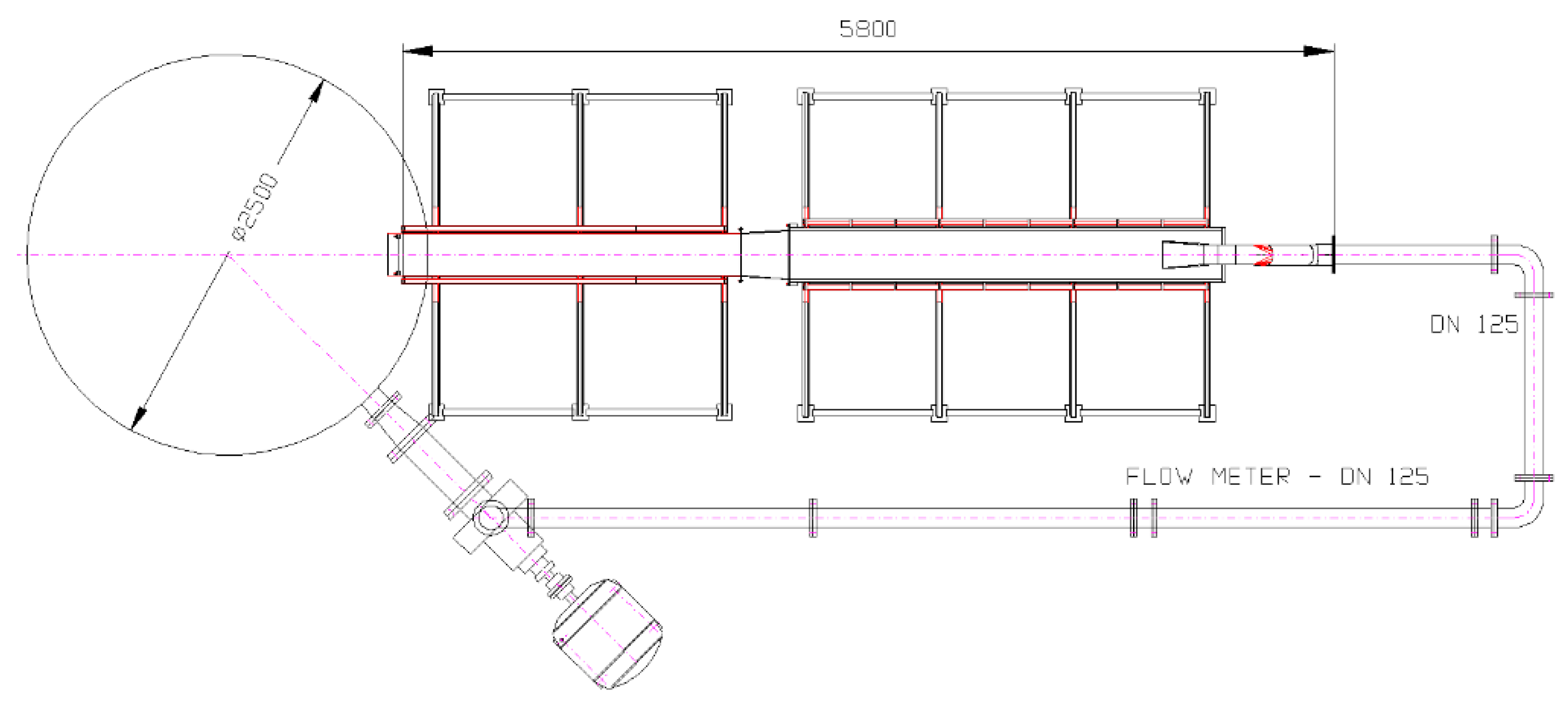
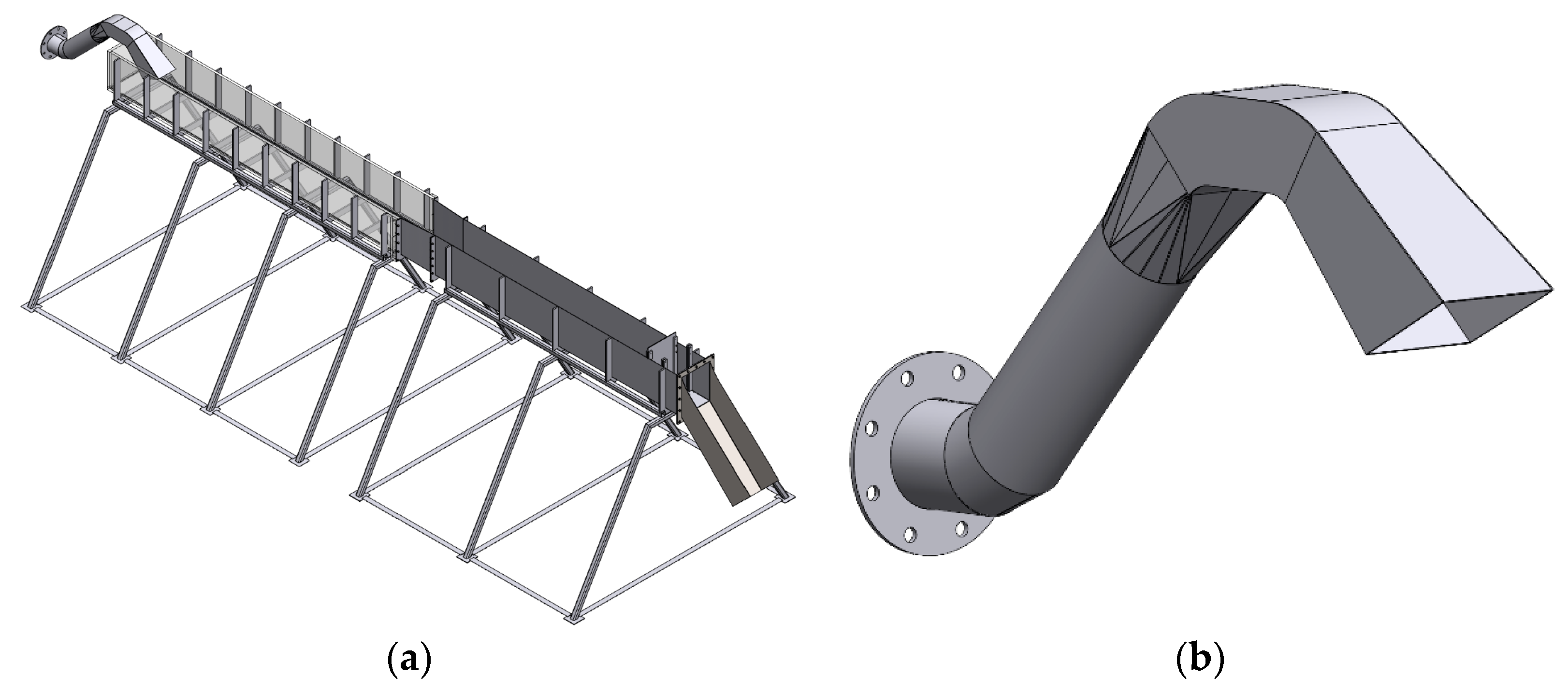
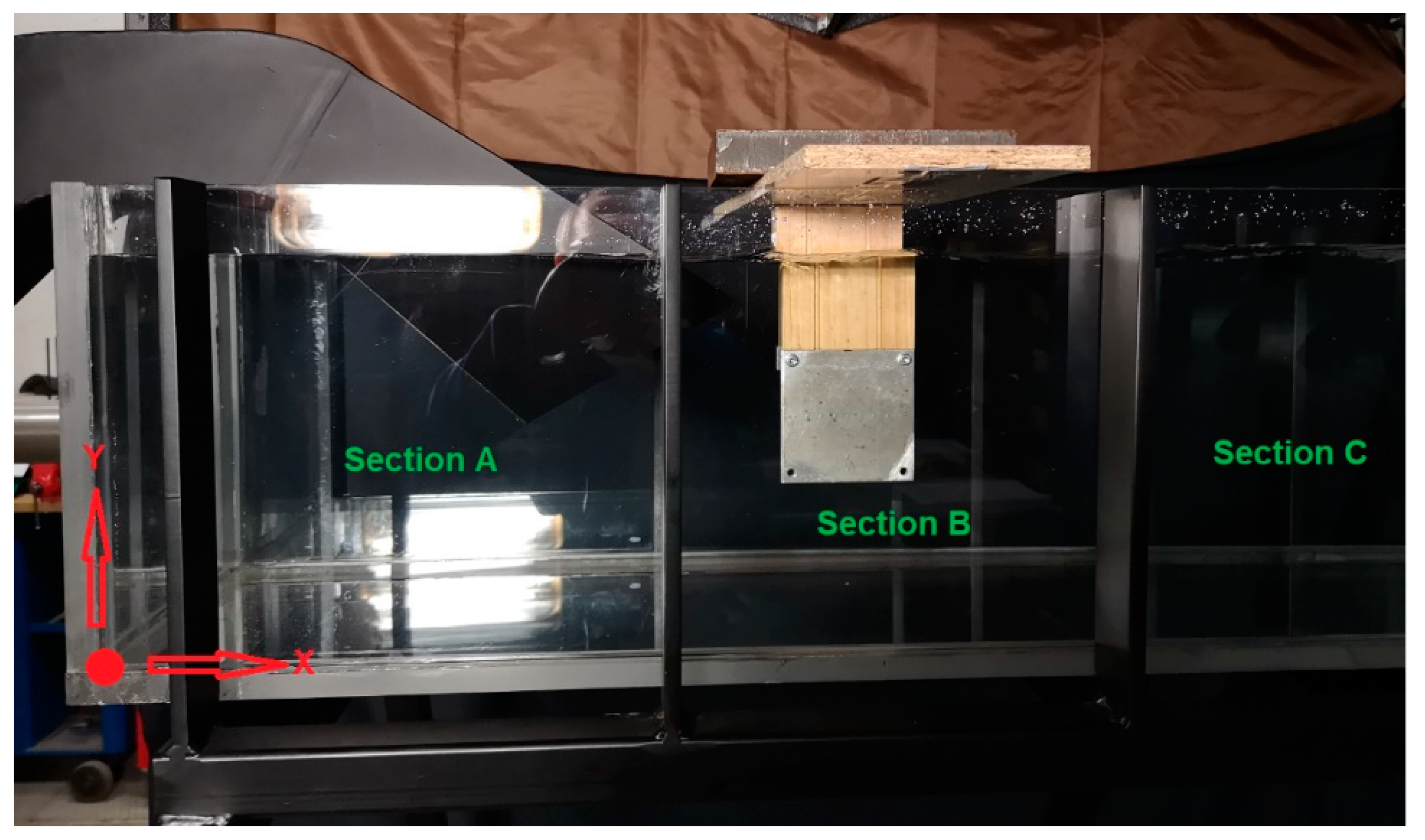
All experiments have been carried out in the water circuit with a free water level, in the hydraulic laboratory of the Centre of Hydraulic Research (Figure 1). The test section is 5 m long, with the sluice gate and a water chute in the rear metal part. The front transparent part of the test section has the dimensions (l × h × w) 2.7 m × 0.37 m × 0.304 m (Figure 2a). The welded siphon (Figure 2b) starts from the flange DN125, then turns to the rectangular cross-section 0.122 m × 0.103 m and ends with the diffuser with an opening angle of 10° in the horizontal direction and 7.4° in the vertical direction. The length of the diffusor is 0.31 m along the upper wall. The cylindrical tank with 2.5 m in diameter has the capacity of 5.9 m3 (Figure 3). Two volume flow rates Qv have been considered: 0.0138 m3/s (with the water level 0.261 m above the floor, measured in the rear part of the transparent section) and 0.0172 m3/s (with the water level 0.268 m above the floor), which correspond to the mean longitudinal velocity in the discharge tank about 0.174 m/s and 0.21 m/s respectively. Both these regimes correspond to the real-life regimes in the already built pumping stations. The aim is the sensitivity analysis of influence of the volume flow rates on the measured and calculated flow structures. The volume flow rate has been measured with the induction flowmeter (accuracy 0.05 L/s) and the mean water level has been controlled by the ultrasonic level transmitter (accuracy 1 mm).
3. Experimental Methods
The start-up regime, when the water is filled with a large amount of air bubbles could not be measured by means of PIV. For the steady state regimes of the siphon performance, the PIV measurements with one camera have been realized (Figure 4). Therefore, the results represent two components of the velocity vectors in the plane of the laser sheet. The measurement apparatus consists of a laser and the CMOS camera by Dantec Company. The laser is the New Wave Pegasus, Nd:YLF, double head pulse type with the light of wavelength 527 nm, the maximal frequency is 10 kHz, the single shot energy is 10 mJ (for 1 kHz) and the corresponding power is 10 W per one head. The camera Phantom V611 with the resolution of 1280 × 800 pixels is able to acquire double snaps with the frequency up to 3000 Hz (the full resolution) and it uses the internal memory of 8 GB for the data storage within a single experiment. The data have been acquired and post-processed using the Dynamic Studio, Matlab and Tecplot software tools [13]. Measurements in both the vertical and horizontal planes have enabled to get a complex view of the flow structures. The vertical planes have been located in the positions z = 0 mm, +/−75 mm and +/−141 mm, where z is the distance from the test section symmetry plane. The horizontal planes have been located at the distance of 10 mm, 135 mm and 170 mm above the test section floor.
The measurements have been done in the Segment A (in front of the siphon), Segment B (location of the main siphon jet) and Segment C (behind the siphon), see Figure 5. The wide-angle objective lens enabled to capture flow pictures with the maximum dimensions about 300 mm × 300 mm, which fits well with the distances between test section steel ribs. For the vertical planes, the 105 mm objective has been applied, the horizontal planes have been visualized with the 35 mm objective. In every segment, the calibration has been performed in one vertical plane (z = 0 mm) and in one horizontal plane (y = 100 mm) using special optical target boards (Figure 5). Both the overall view of the Segments A–C and details of flow close to the siphon walls have been captured, including time-averaged and instantaneous results. The instantaneous results have been captured with the frequencies of 100–250 Hz; the time-averaged results have used frequencies 10–20 Hz. In the investigated flow areas, there are quite high velocity gradients. In the local areas with very low velocities, we can expect an increased level of uncertainty. Inside local areas with the velocities in the order of about 1 m/s, the accuracy of velocity measurements is about 1–2% of the maximum velocity.
4. Numerical Simulations
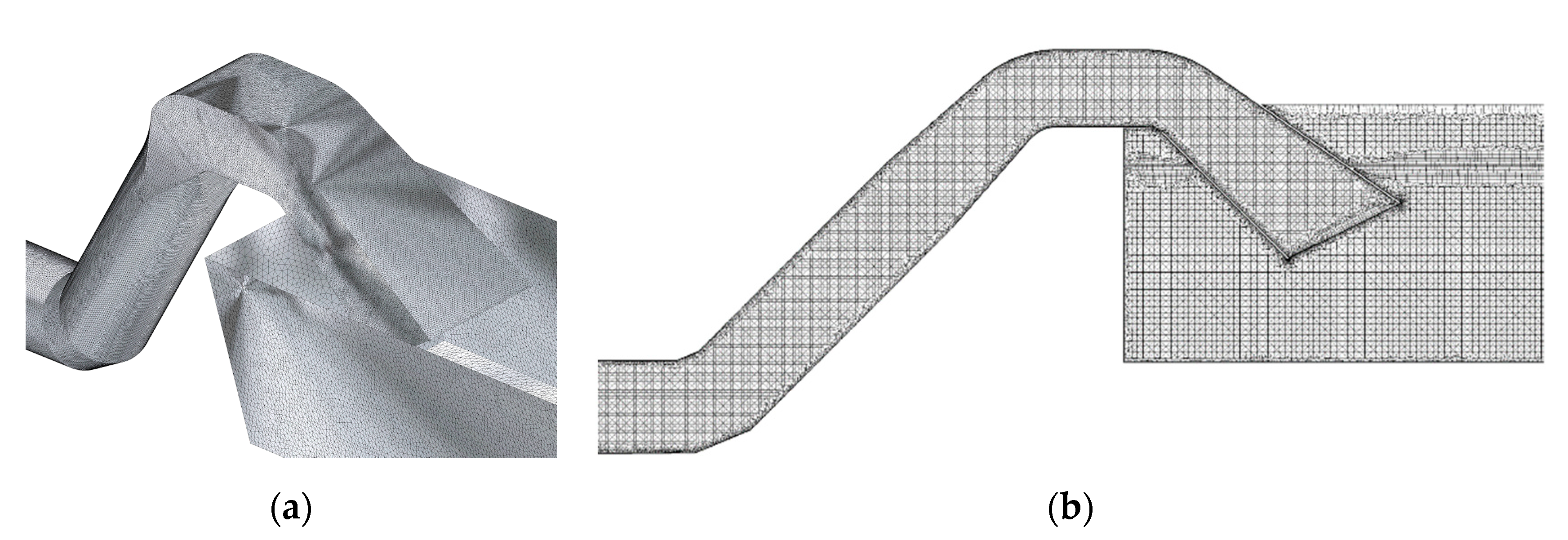
All calculations in the discharge object with the siphon have been carried out by means of the CFD software ANSYS CFX release 19.2. The free-surface flow modelling including the gravity effects is based on the VOF method evaluating the volume fraction of each fluid. A non-homogenous model of the multiphase flow has been applied with different velocities for the water and air fractions. In this study the unstructured computational grid with prismatic elements inside the boundary layers has approximately 10 million nodes (Figure 6), which enables to preserve sufficiently low values of y+ calculated at the first grid point away from the solid walls and to reach a sufficiently isotropic grid with acceptable aspect ratios close to the walls. The maximum distance of the neighboring grid points is about 3 mm, which enables to capture the turbulent vortices larger than 10 mm. It is practically impossible to optimize the computational grid from the point of y+ values as the wall shear stress changes dramatically in time with the changing pattern of separation and attachment regions. In our case the values of y+ monitored in time have remained close to 1 on the majority of solid surfaces.
As mentioned above, the transient phenomena during the start-up phase of the pumping station as well as the experimental discharge object with the welded siphons have been studied numerically in [4] using the SAS and DES scale resolving simulations. Though the DES simulations provided better resolution of vortical structures, the SAS simulations showed much better robustness and better predictions of frequencies of unsteady phenomena. That is why the fundamental calculations in this study are based on the SAS simulations, with the time step of Δt = 0.005 s. Nevertheless, these calculations are also compared with the shear stress transport (SST) turbulence model based unsteady Reynolds-averaged Navier–Stokes equations (URANS) calculations (with the time step of Δt = 0.01 s), which provide some time-averaging (the Reynold’s one) of results, though they are fully unsteady in their nature.
The computational domain includes all the three-dimensional geometry of the discharge object including the siphon with its walls. No symmetry plane has been applied. To set correctly the inlet boundary conditions, the computational domain has been extended with a straight piping DN125 of the length 0.75 m (six diameters) in front of the flange (which corresponds to the experiment). The boundary conditions are based on the prescribed volume flow rate at the inlet and the static pressure distribution at the outlet. The initial calculations employed the URANS equations with the standard SST turbulence model and then switched to the SAS simulations. The momentum equations have employed the high-resolution scheme while the first order scheme has been used for the turbulence numerics. The time discretization has employed the second order backward Euler scheme.
All the simulations are based on the constant property fluids. It means, that both the water and water vapor are taken as incompressible, with constant densities and constant temperatures.
5. Results
In this paragraph, some selected results of the PIV measurements and the CFD simulations are presented. The complete database is collected at the Centre of Hydraulic Research as well as at the Institute of Thermomechanics, Czech Academy of Sciences, the contact emails are provided above.
5.1. PIV Experiments
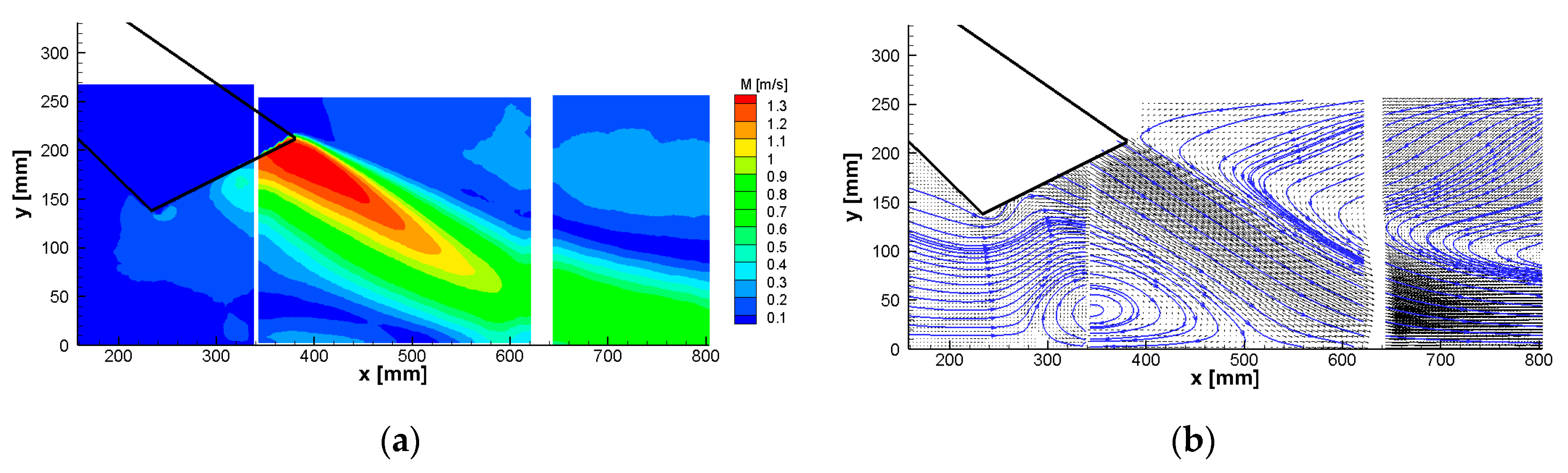
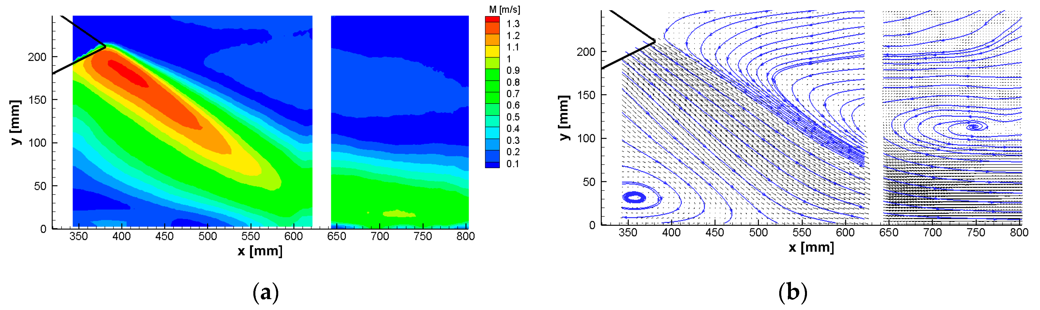
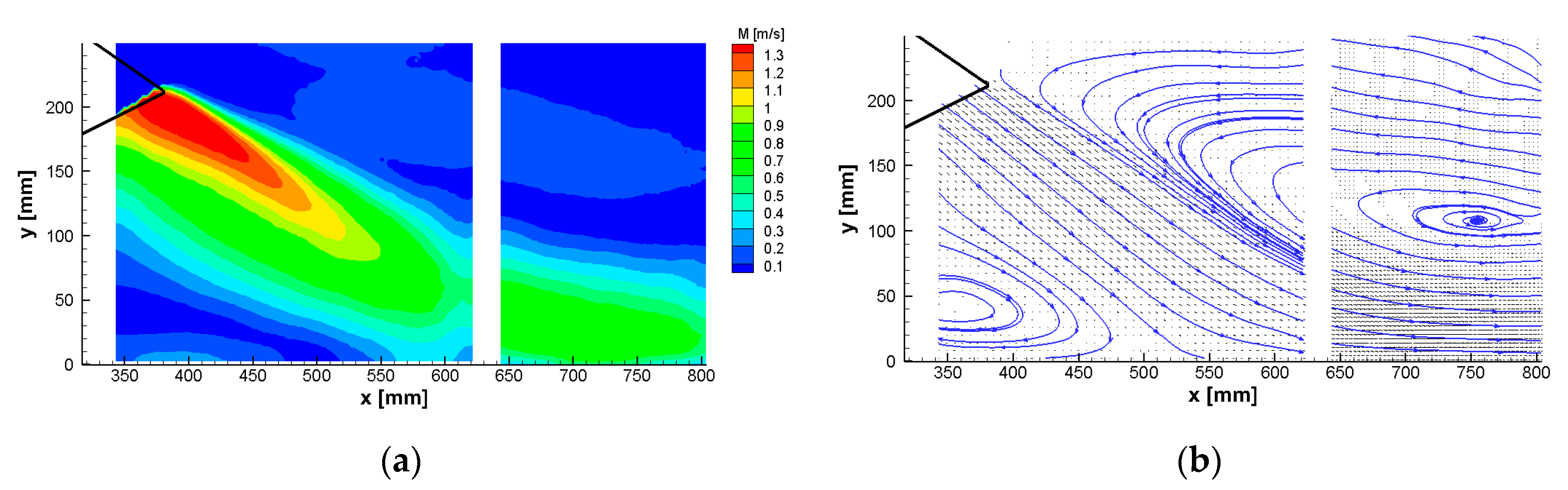
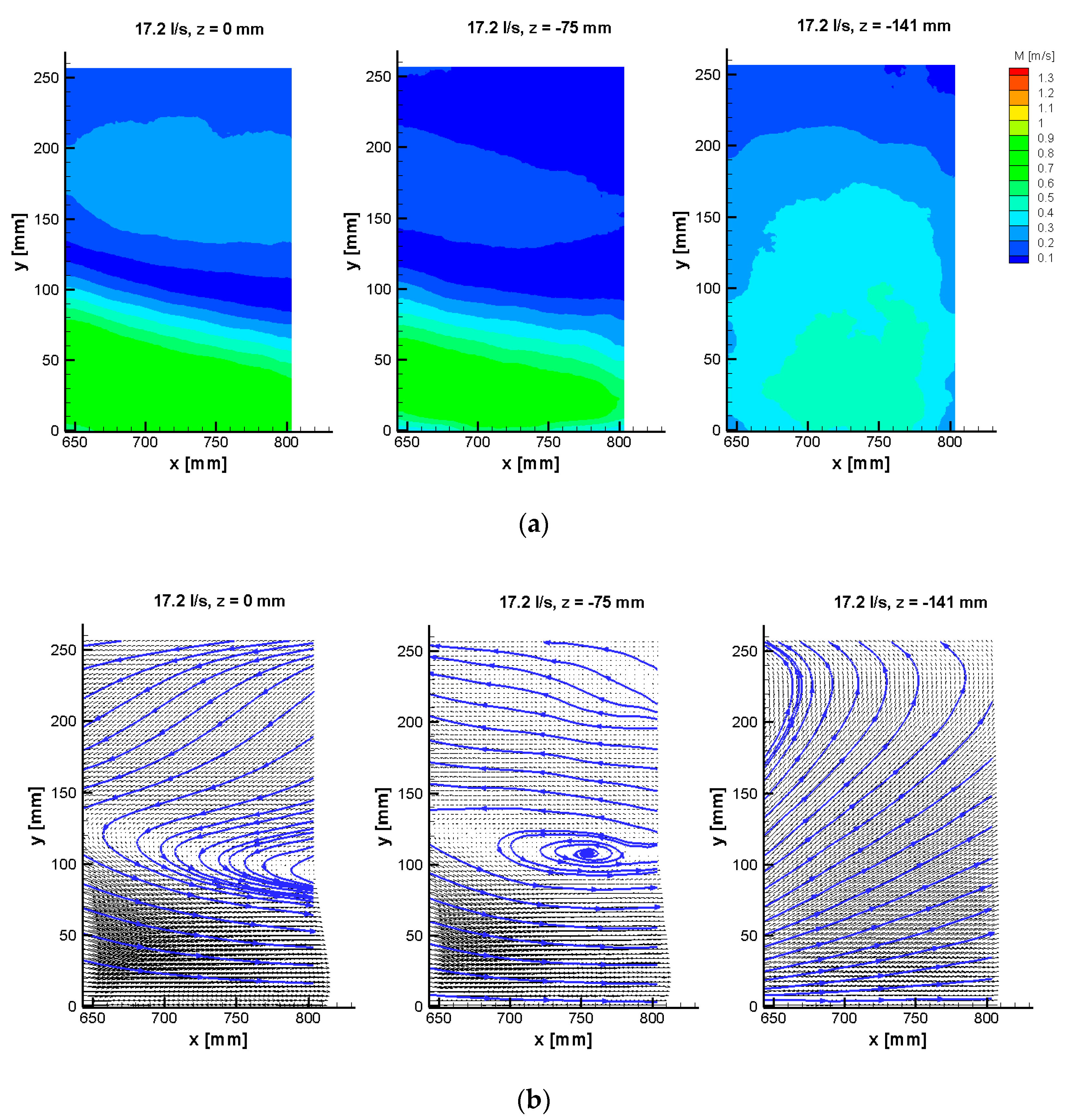
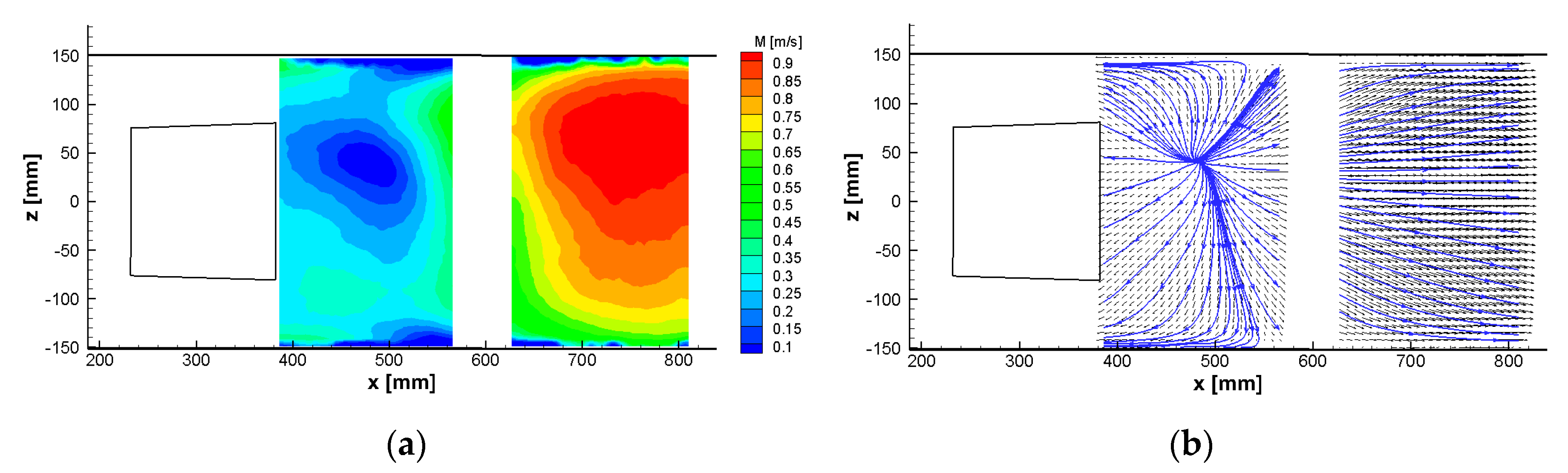
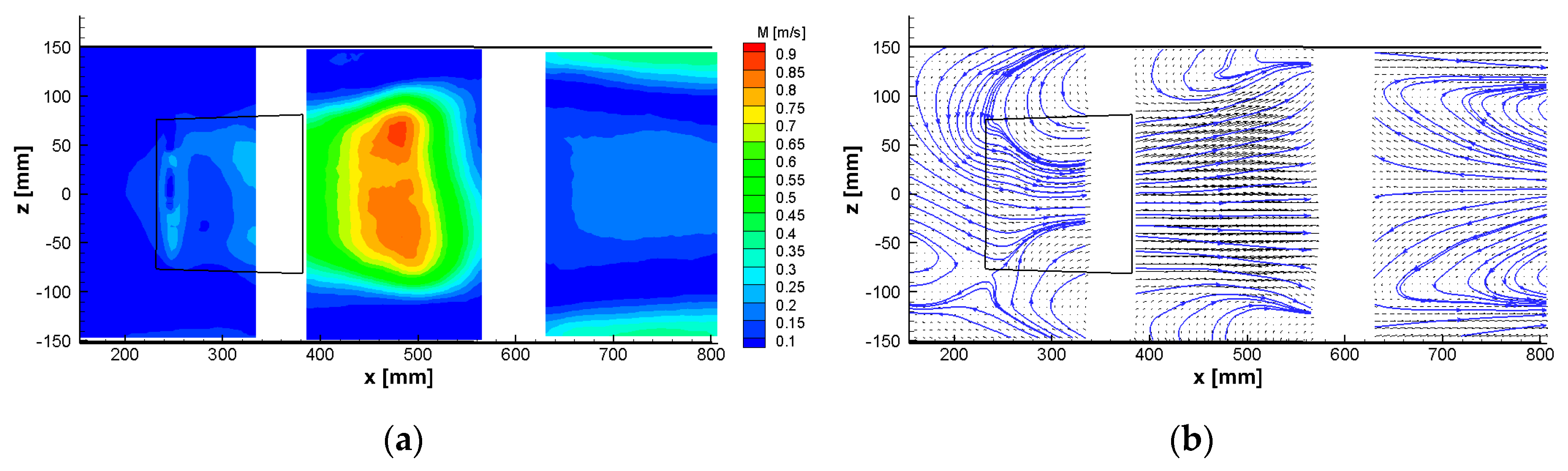
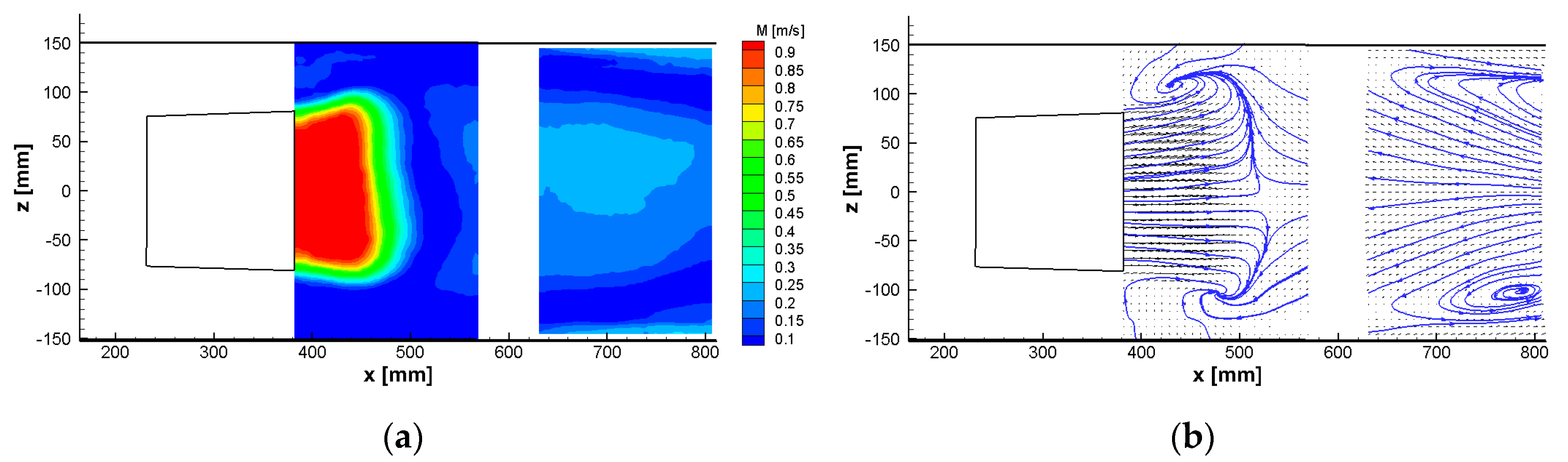
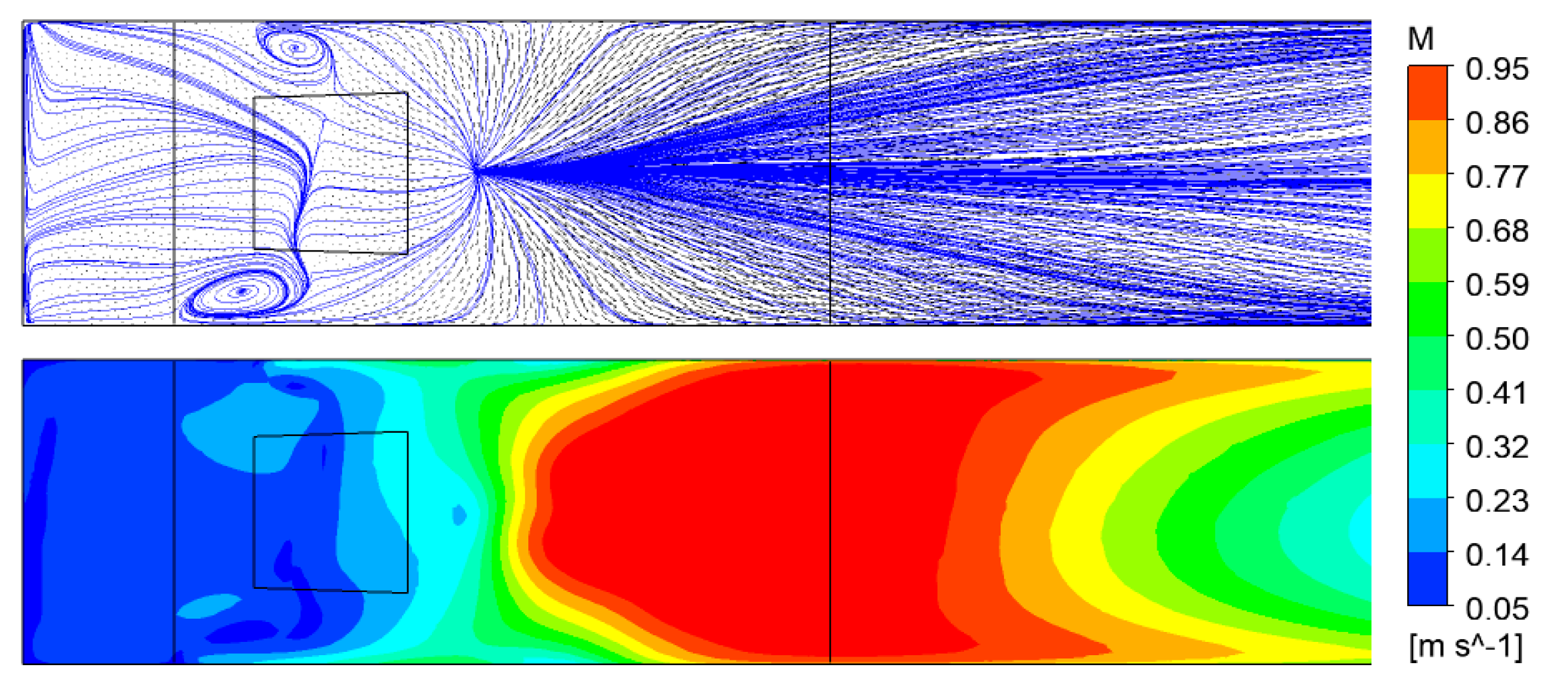
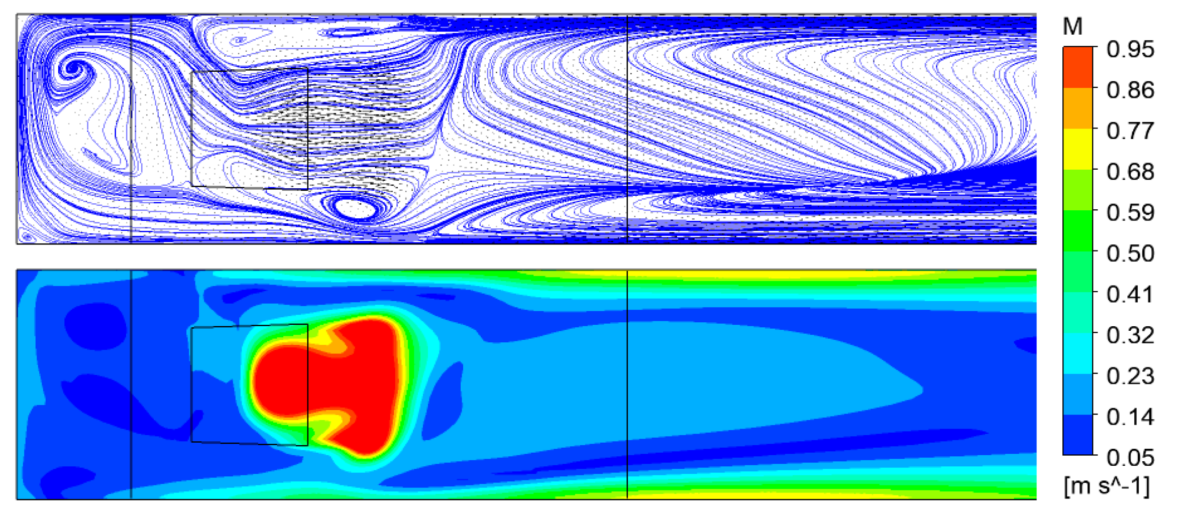
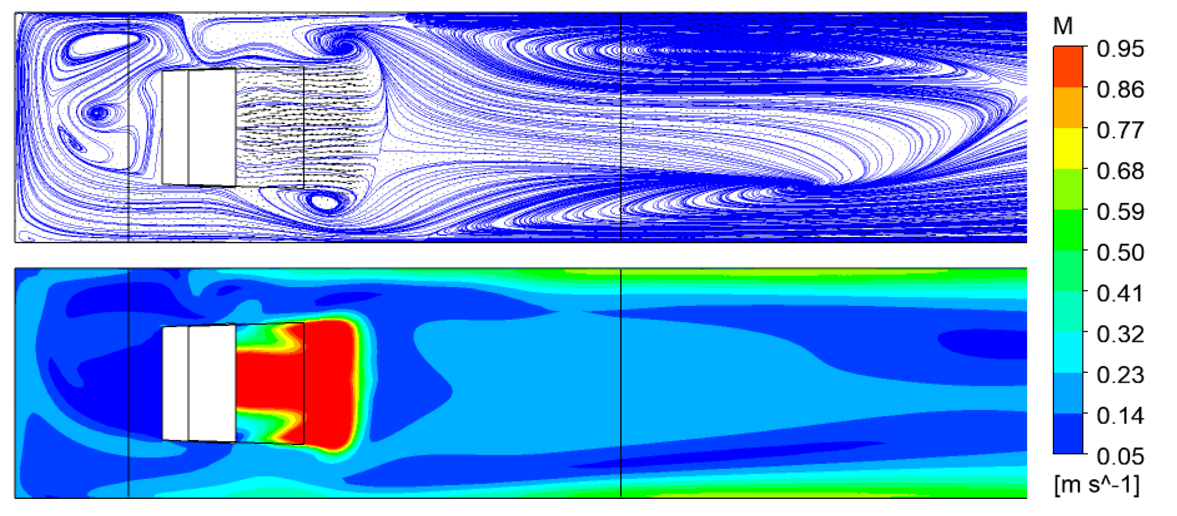
During the experiments, the (two-dimensional) velocity vector magnitude (the symbol M in corresponding figures) has been evaluated, together with the individual velocity components, variances and vector lines with the singular points. The general term “vector lines” is used in the description of results as “streamlines” are strictly “vector lines of the instantaneous velocity fields in 3D”, which is not the case of the time-averaged velocity fields in 2D. Not all data can be presented because of limited space of the article. Moreover, because for both measured flow rates the topology of the flow phenomena is the same, with the difference just in the velocity magnitude (as it will be shown hereinafter), only the results for the volume flow rate of 0.0172 m3/s (with a higher relative accuracy) are considered. Figure 7, Figure 8 and Figure 9 show the (two-dimensional) magnitude of velocity and the vector lines in the vertical planes z = 0, 75 and –75 mm obtained from the time-averaged results. The primary flow structure is a water jet, which dominates in the upper part of the siphon outlet, accompanied with a backflow and a strong vortex just below the siphon outlet. The jet tears down the water above the siphon outlet, with a distinct shear layer. In the vertical planes z = 75 and –75 mm, a large secondary vortex can be located behind the jet, above the nodal point of attachment (Figure 8 and Figure 9). The flow is weakly asymmetrical in the vertical planes z = 75 and –75 mm, but it is rather insignificant in these figures. Figure 10 shows the flow in the vertical planes z = 0, −75 and –141 mm in the Segment C obtained for the time-averaged results. It can be seen that the secondary vortex located behind the jet is not fully perpendicular to the test section plane of symmetry and its core can be detected only in the vertical planes z = 75 and –75 mm. The asymmetry of the flow can be visually registered much better in the horizontal planes. In Figure 11, the flow in the horizontal plane y = 10 is shown. The dominant structure here is the nodal point of attachment. It can be seen, that this singular point is shifted about 50 mm from the test section centerline. It is very important to note, that the nodal point of attachment is a highly unstable node. Its position is unsteady and any small deviation in the test section geometry causes the asymmetry of the experimental results. It is in contrast with the numerical simulations, which consider the test section geometry perfectly symmetric and without any influence of external (e.g., Coriolis) forces. Figure 12 and Figure 13 show the flow in the horizontal planes y = 135 mm and 170 mm. The flow asymmetry is decreased here a little bit, which indicates, that the main source of the asymmetry is located near the floor.
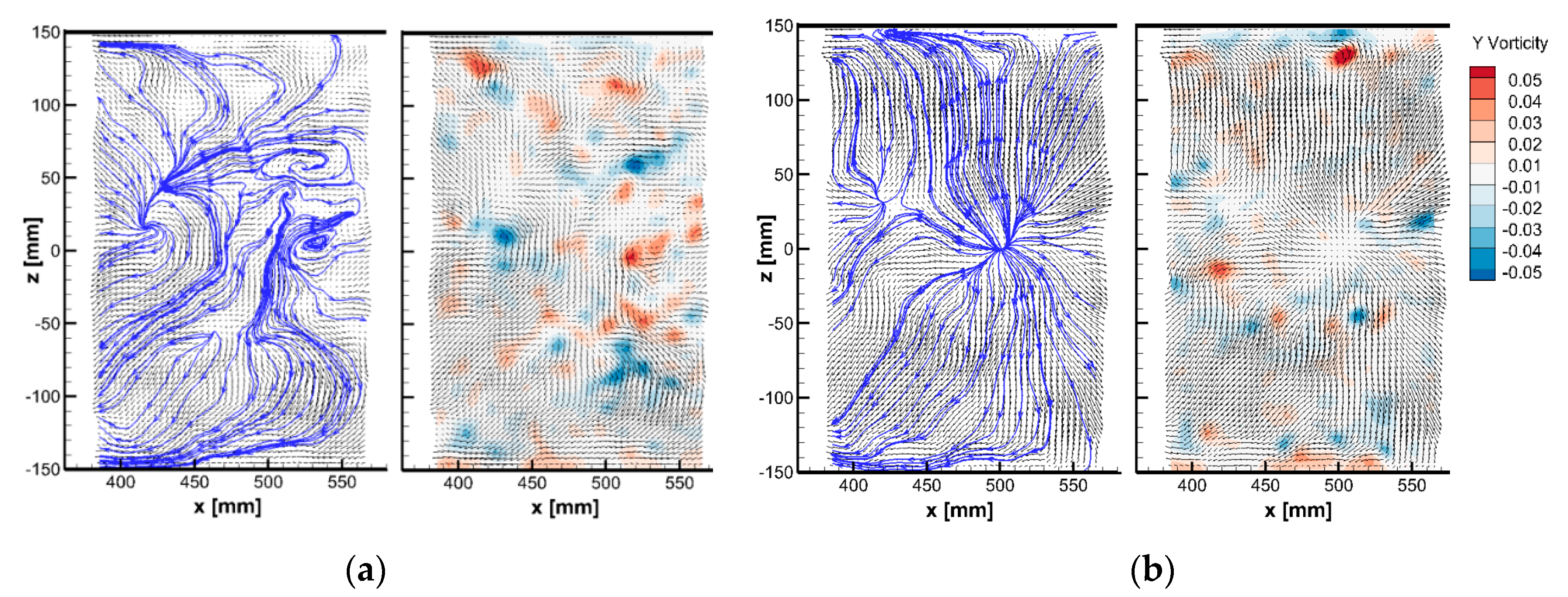
The instantaneous flow structures in the horizontal plane y = 10 mm are shown in Figure 14. In some instants, there is a complex system of singular points replacing temporarily the picture of one dominant nodal point of attachment. On the other hand, in the other instants, this dominant nodal point can be clearly recognized and apparently it is not necessarily shifted from the test section centerline all the time.
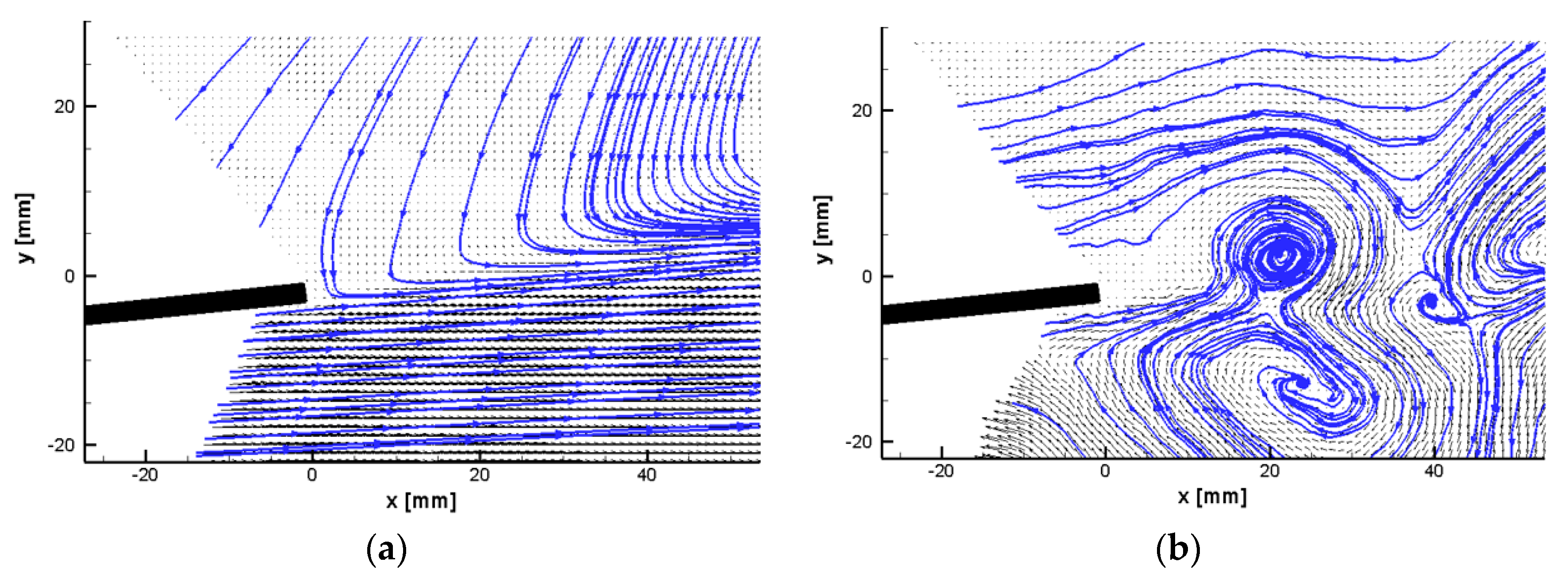
Figure 15 shows the flow in the shear layer behind the upper siphon wall in the vertical plane z = 0 mm. Pictures and the coordinate system are in this figure rotated by 37° against the horizon. Unsteady vortices behind the wall edge can be found in the shear layer.
As it has been already mentioned, not all data are presented, because for both measured flow rates (0.0138 m3/s and 0.0172 m3/s) the topology of the flow phenomena is the same, including the same asymmetries in the flow fields. It is partially demonstrated in Figure 16, which shows the flow structures measured at the volume flow rate of 0.0138 m3/s and can be compared to the results in Figure 7 and Figure 8. For clarity, Figure 16 is the only one with the volume flow rate of 0.0138 m3/s.
5.2. CFD Simulations
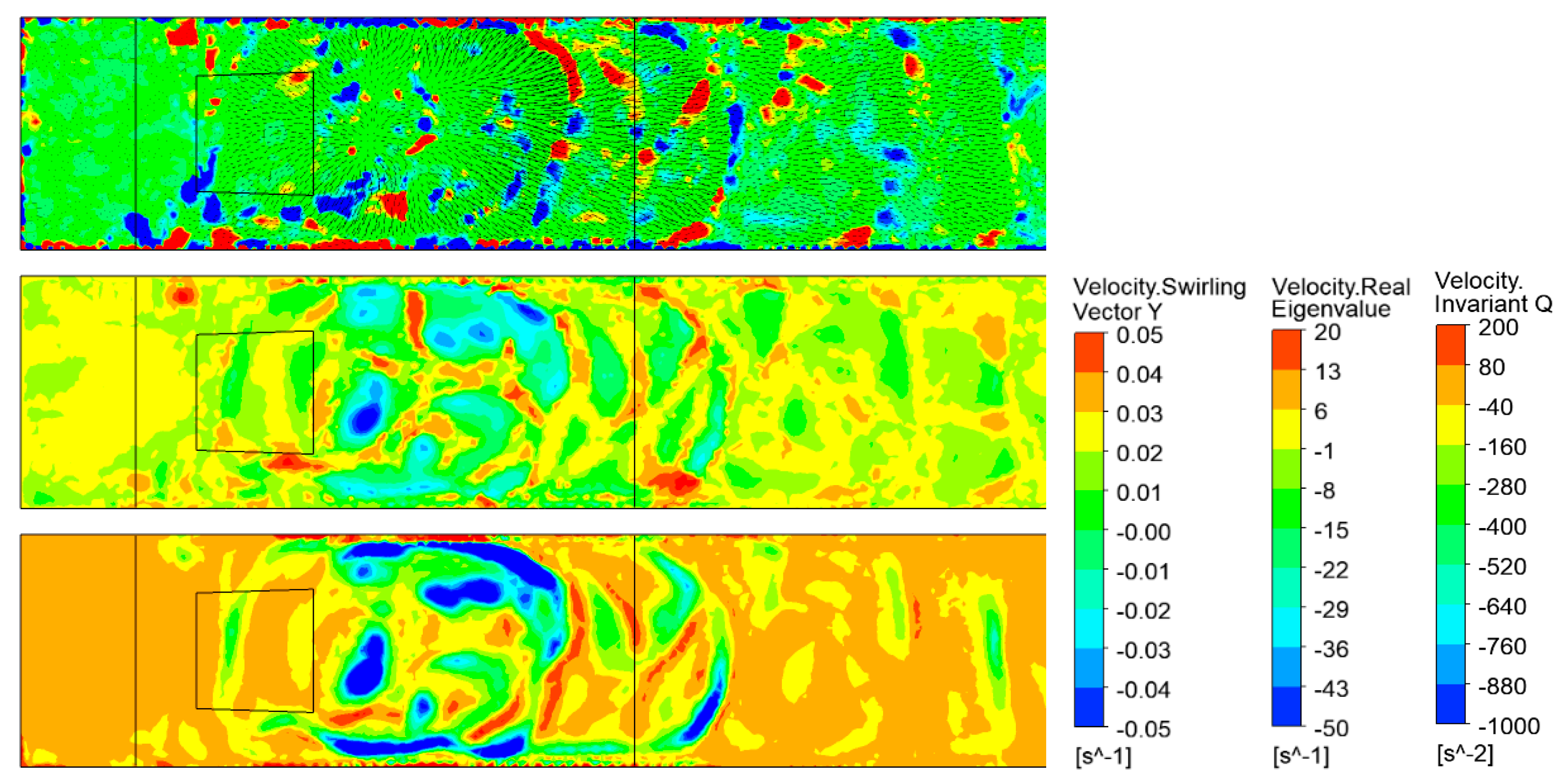
Similar to the experiments, the (two-dimensional) velocity vector magnitude has been evaluated from velocity components, together with the vector lines and singular points. Moreover, some criteria which enable to visualize the vortical structures (like the vorticity, velocity real eigenvalue or Q invariant [14,15]) are used for unsteady results. As mentioned for the measurements, only the results for the flow rate of 0.0172 m3/s are presented.
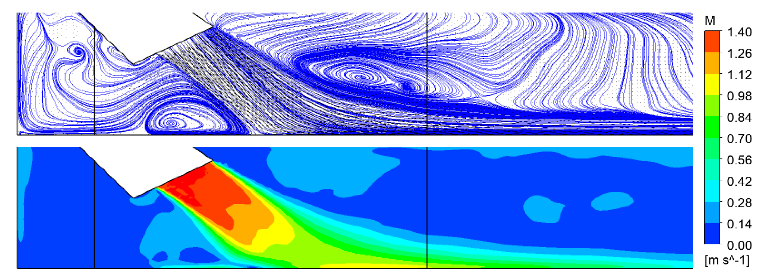
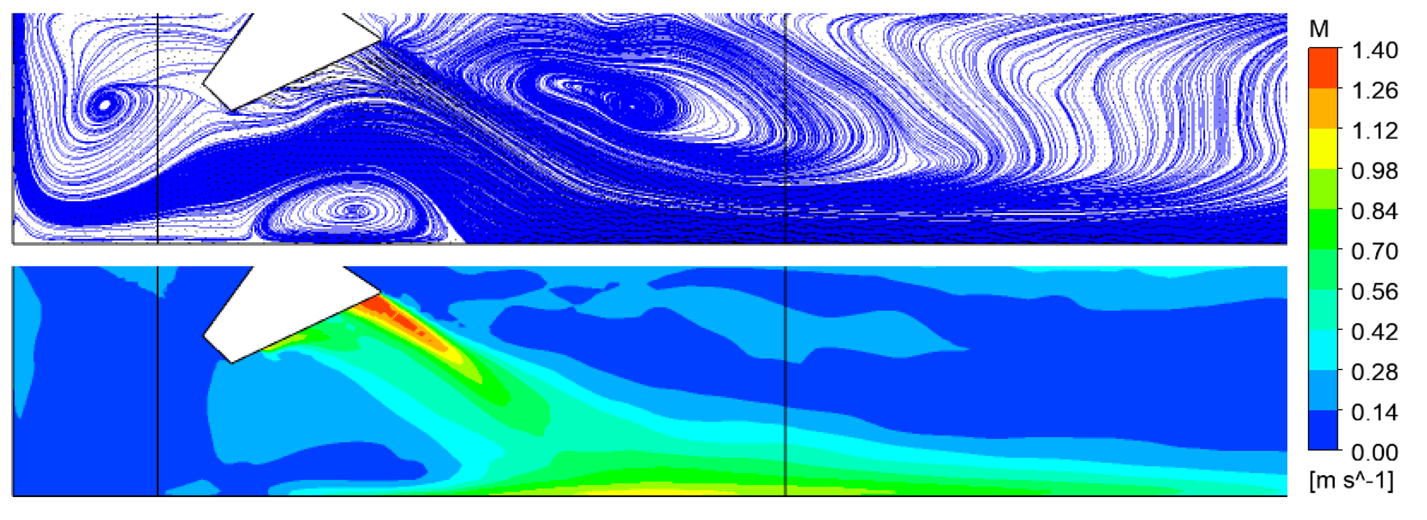
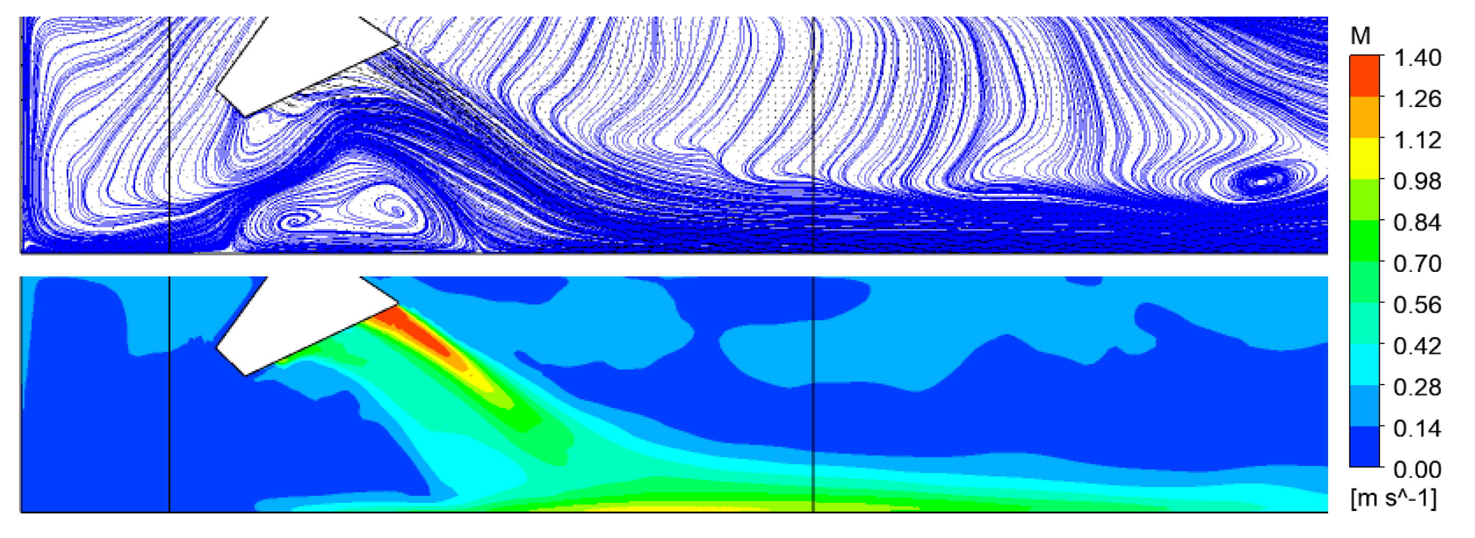
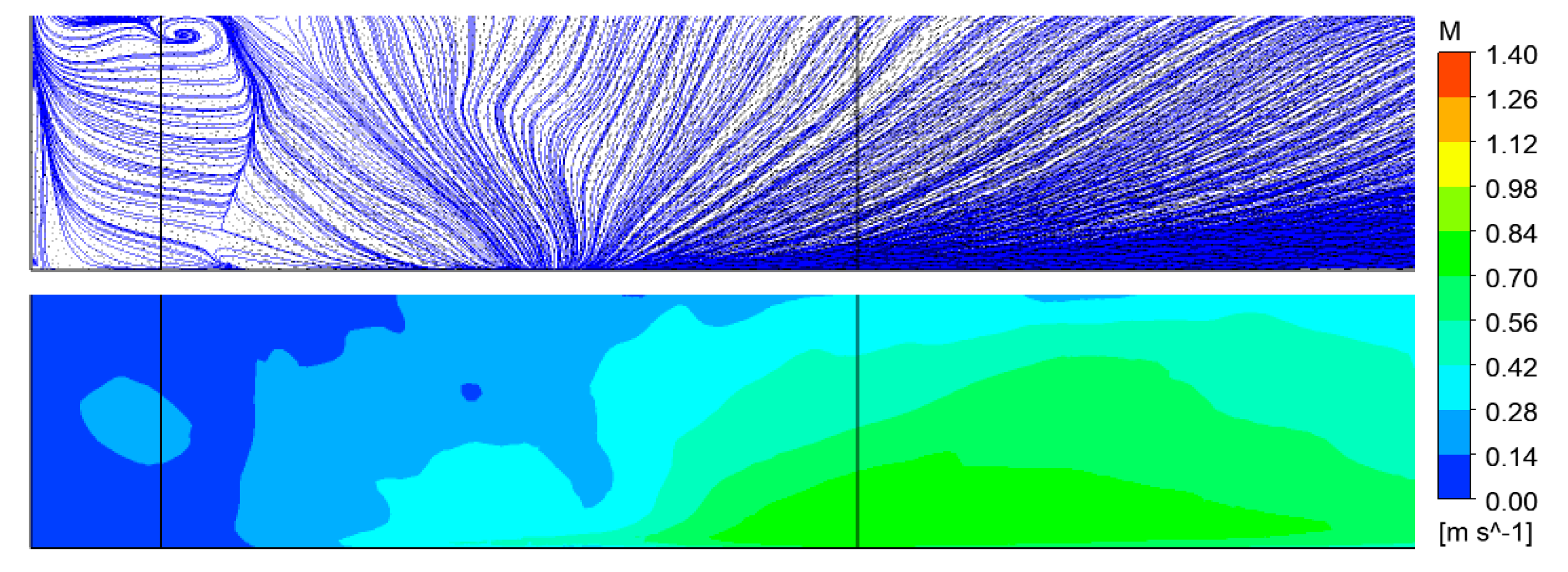
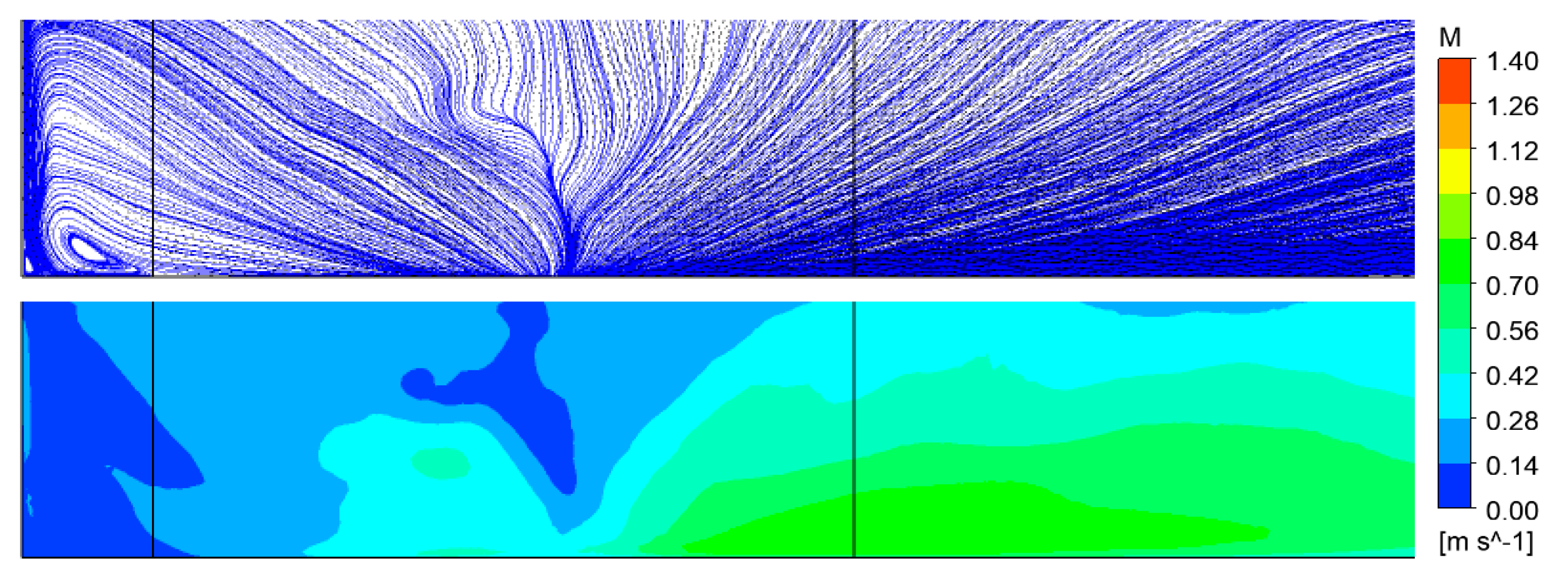
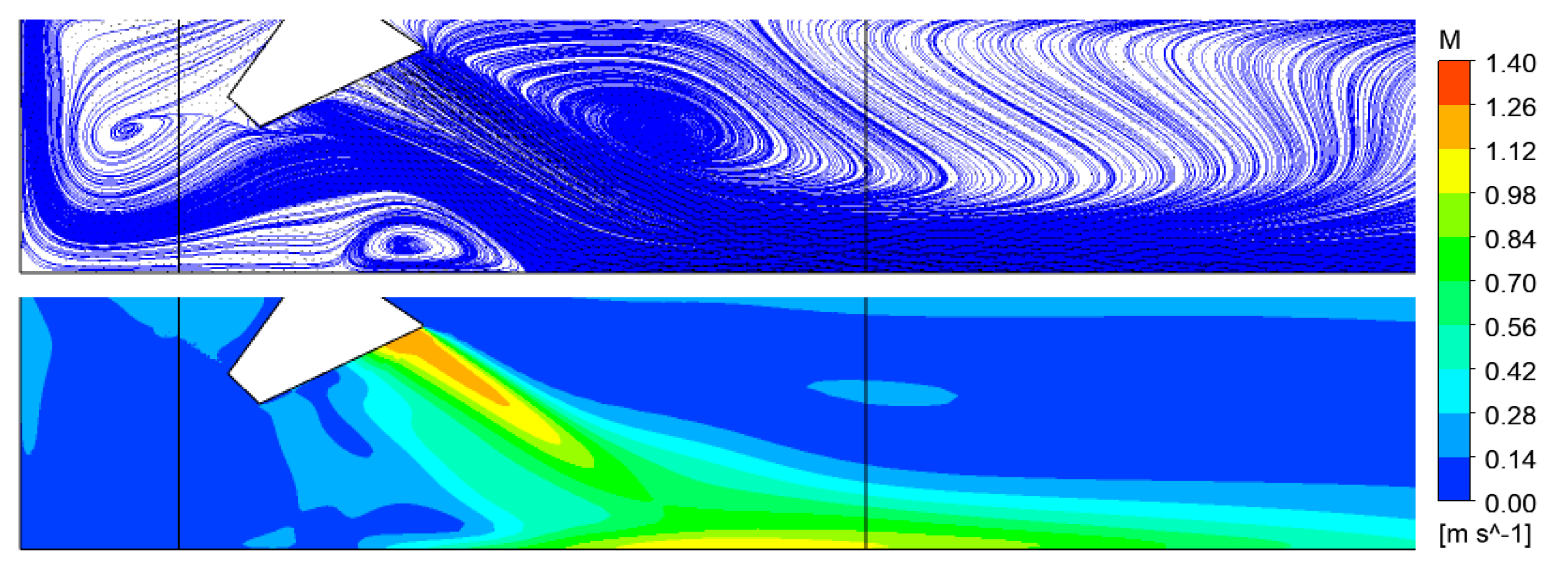
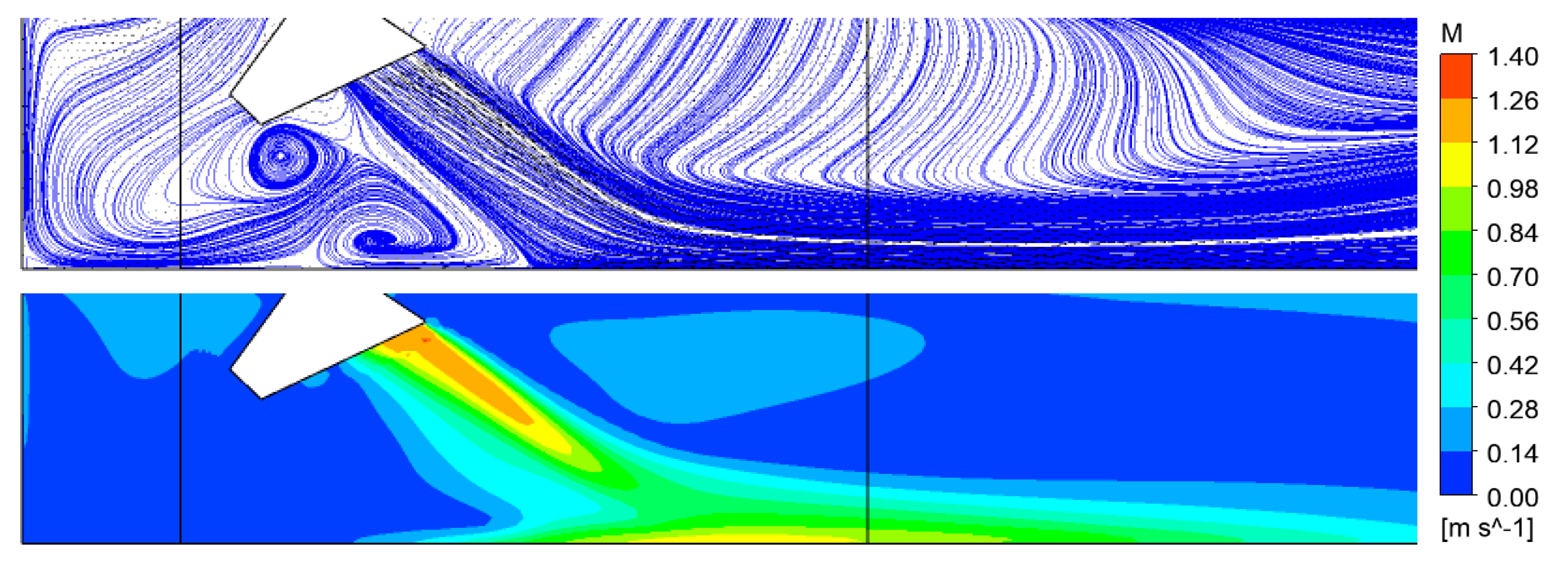
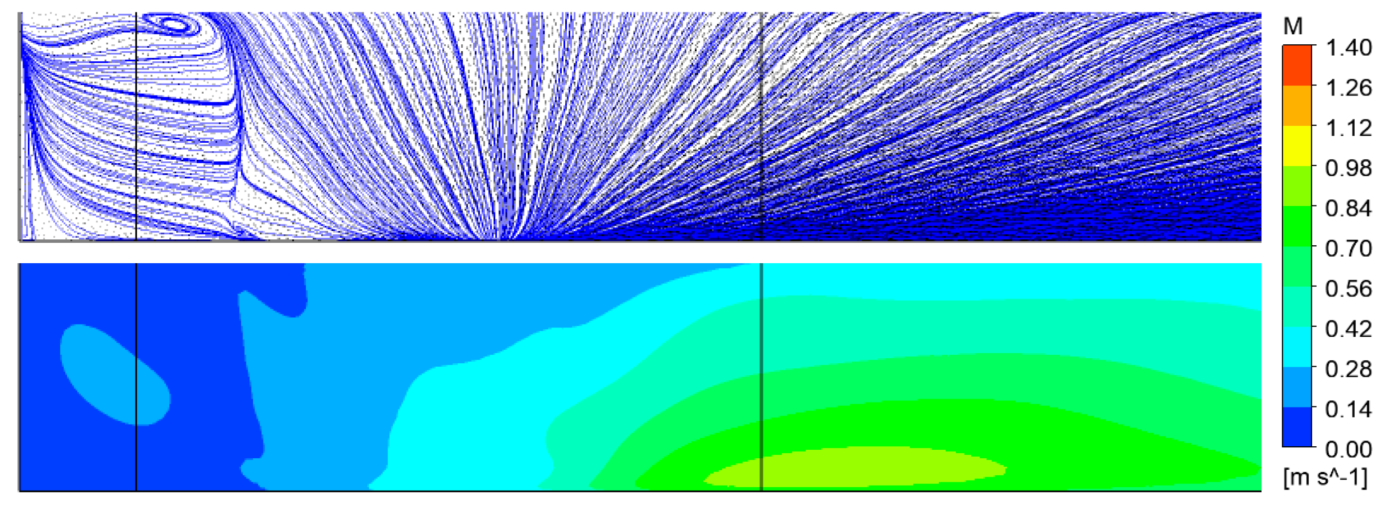
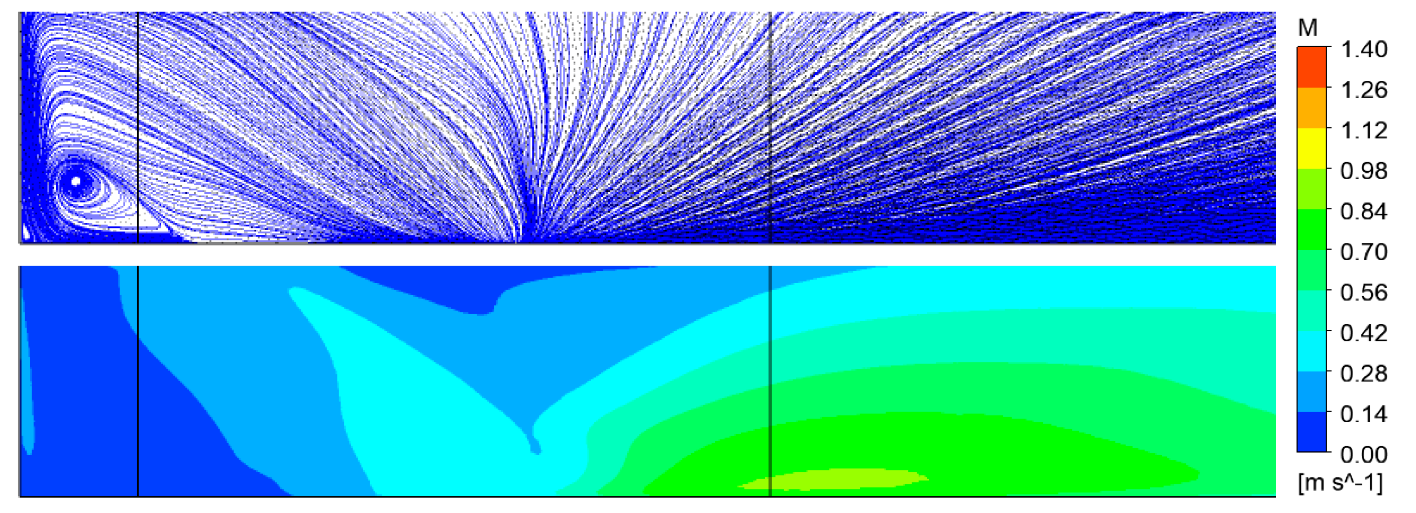
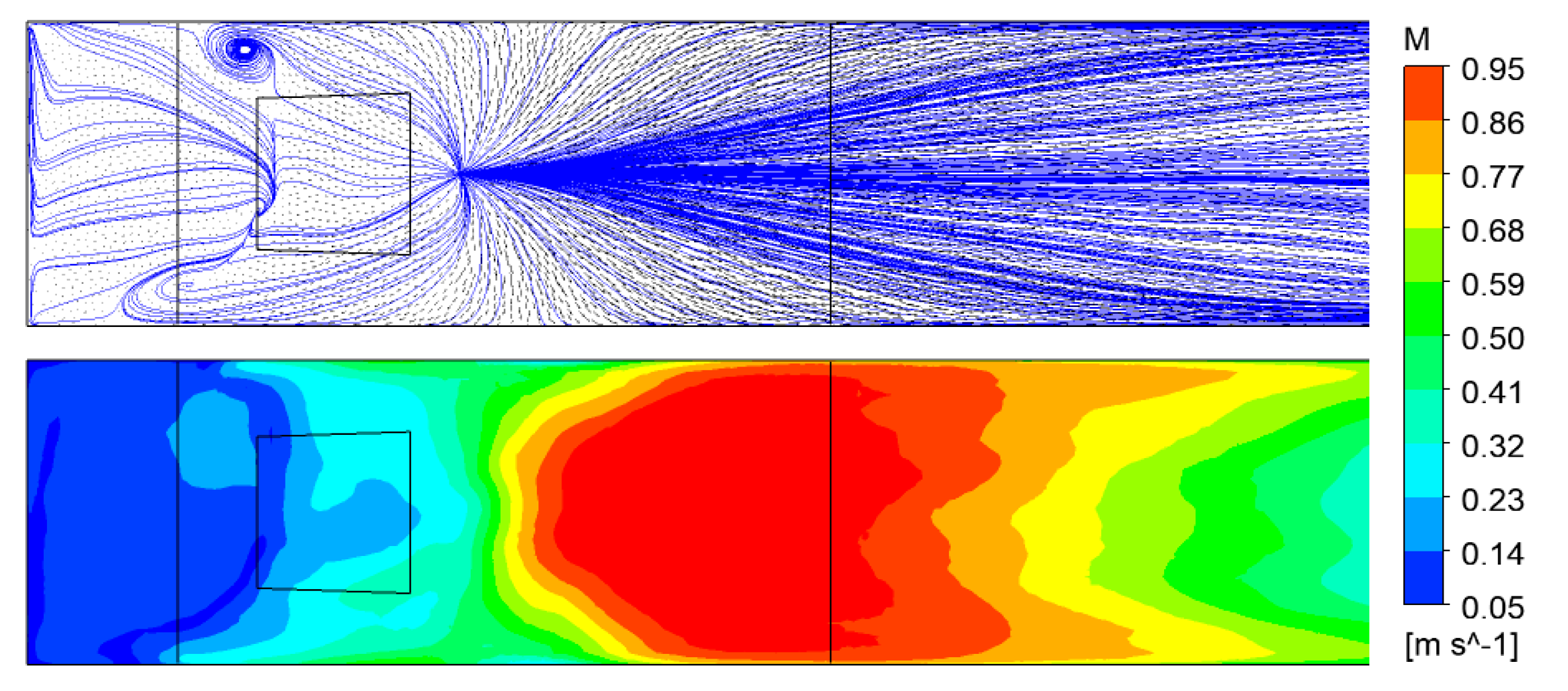
Figure 17, Figure 18, Figure 19, Figure 20 and Figure 21 show the (two-dimensional) magnitude of velocity and the vector lines in the vertical planes z = 0 mm, ±75 mm and ±141 mm obtained with the SAS turbulence model for the time-averaged results. To enable a better comparison with the experimental data, each picture includes indicative lines with the x-coordinates x = 151 mm and 806 mm, which frame the full range of experiment. Though the geometry of the computational domain is perfectly symmetric, the time-averaged results show an asymmetry, especially in the vertical planes z = ±75 mm. There could be several reasons, among them the asymmetric unstructured computational grid or not sufficient size of data files can play the most important role. Nevertheless, a similar asymmetry (including the topology of the asymmetric flow structures) can be found in the time-averaged results obtained with the SST turbulence model as could be seen in Figure 22, Figure 23, Figure 24, Figure 25 and Figure 26. Concerning the horizontal planes (Figure 27, Figure 28, Figure 29, Figure 30, Figure 31 and Figure 32), we can see the asymmetry of the time-averaged results especially in the plane y = 135 mm behind the primary jet. Still, the jet itself is surprisingly symmetric.
It is difficult to quantify and compare the asymmetry of the presented results obtained from the experiments and from the numerical simulations. The asymmetry is an imperfection of the specific experimental apparatus and the mathematical model. For each, the imperfection reason can be different. However, it must be considered, that the investigated phenomena are highly turbulent and unsteady in their nature. Both in the experiment and numerical simulations, the flow in the siphon-based discharge object behaves like the Hopf bifurcation, so, any asymmetry perturbation breaks the global solution symmetry. From the point of view of the visualized results, the numerical simulations show a higher degree of asymmetry.
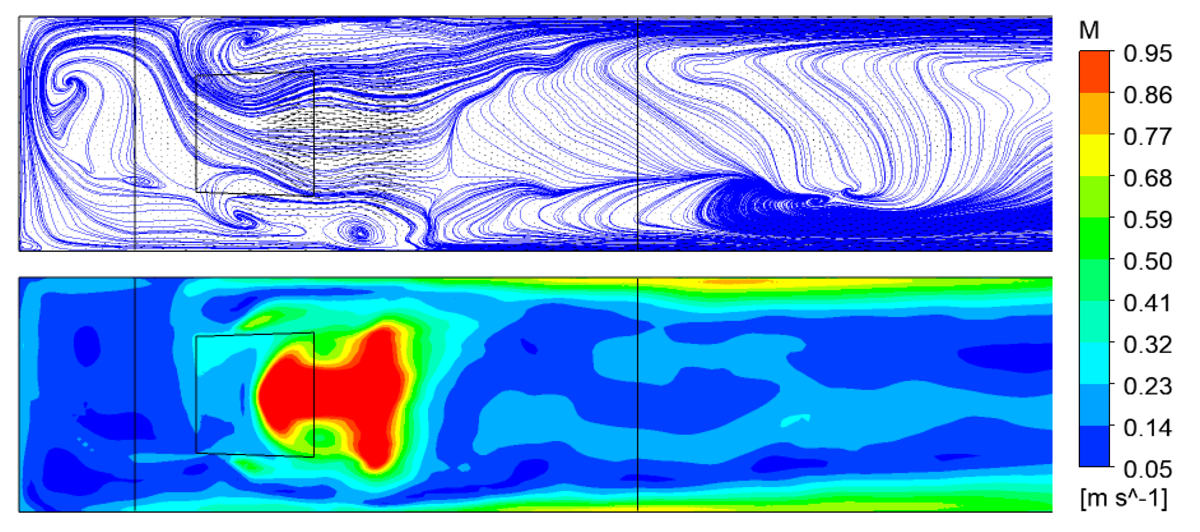
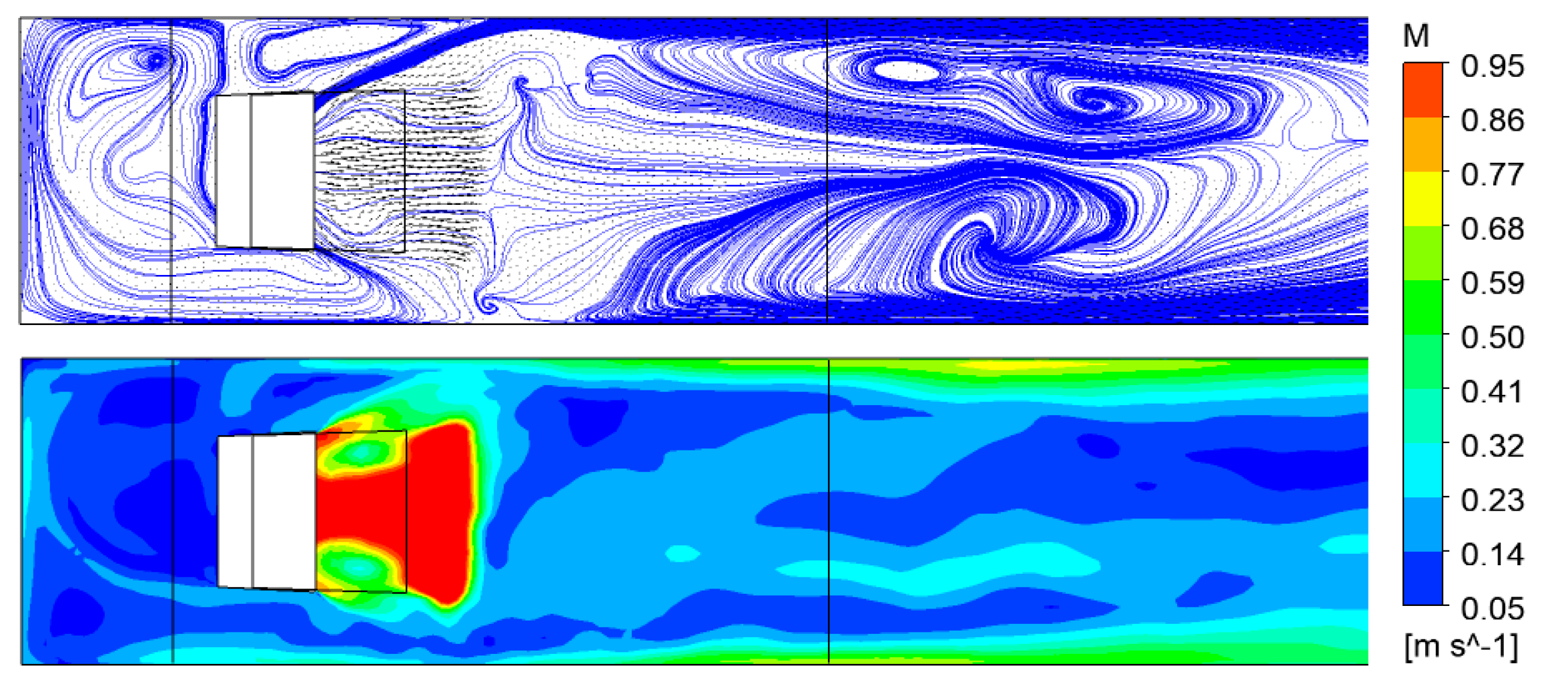
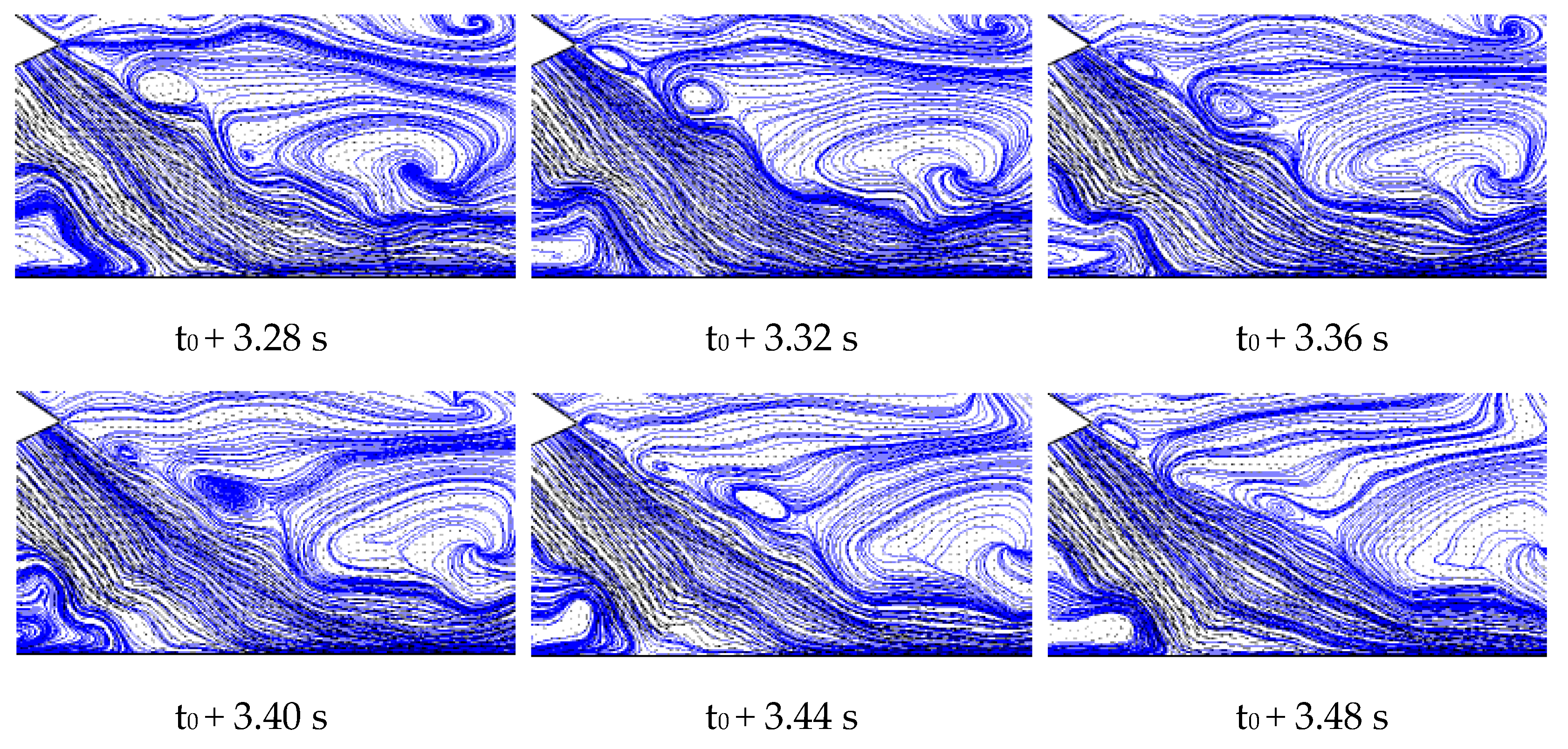
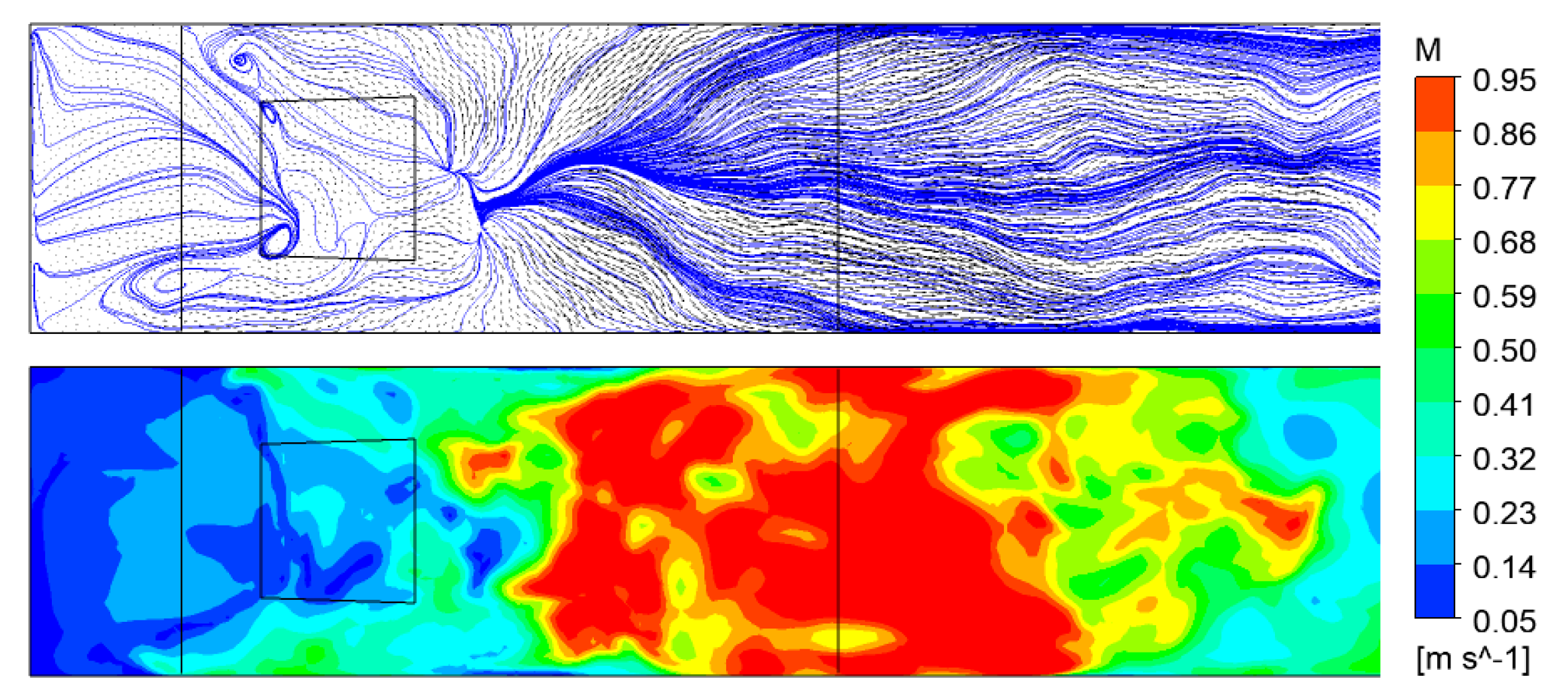
Large turbulent eddies calculated in the vertical plane z = 0 with the SAS scale resolving simulations can be seen in Figure 33 and Figure 34. The highly unsteady vortices can be found especially in the shear layer behind the upper siphon wall. They are shedding with the dominant frequency about 5.2–6.3 Hz (Figure 35). Figure 36 shows (similar to Figure 15) in detail the flow in the shear layer behind the upper siphon wall in the vertical plane z = 0 mm, calculated with the SAS turbulence model. In this figure, pictures and the coordinate system are rotated by 37° against the horizon. The smooth time-averaged shear layer can be seen on the left, unsteady vortices behind the wall edge can be found in the shear layer on the right-hand side. Similar (but much less pronounced and less regular) vortices can be found in the CFD analysis based on the SST model (Figure 37).
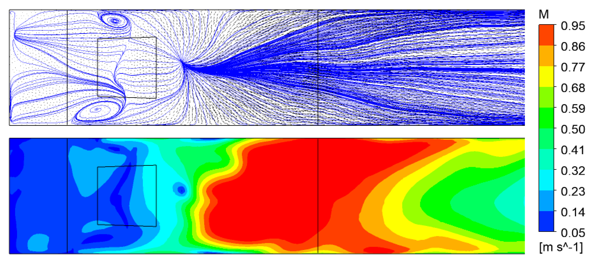
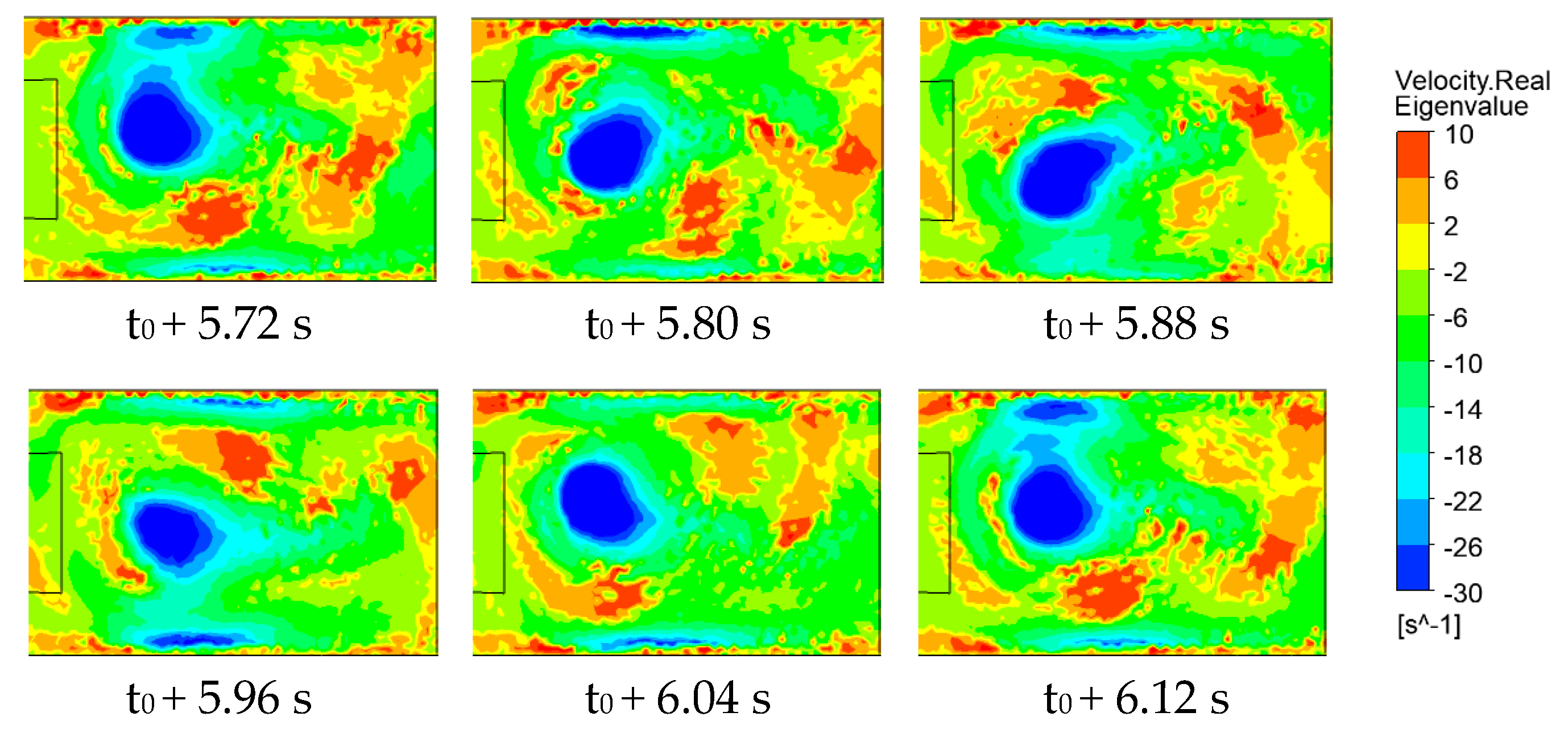
The unsteady flow close to the floor calculated with the SAS turbulence model can be seen in Figure 38 and Figure 39. Similarly to the experiments, the dominant structure here—the nodal point of attachment—can be replaced by a structure of connected singular points. Typically, one to three nodal points can be observed. This structure is periodically moving in the stream-wise and span-wise directions with the frequencies, which will be discussed later. Concerning the SST based simulations, they give one nodal point, moving also in the stream-wise and span-wise directions with the dominant frequency of 2.5 Hz (Figure 40 and Figure 41).
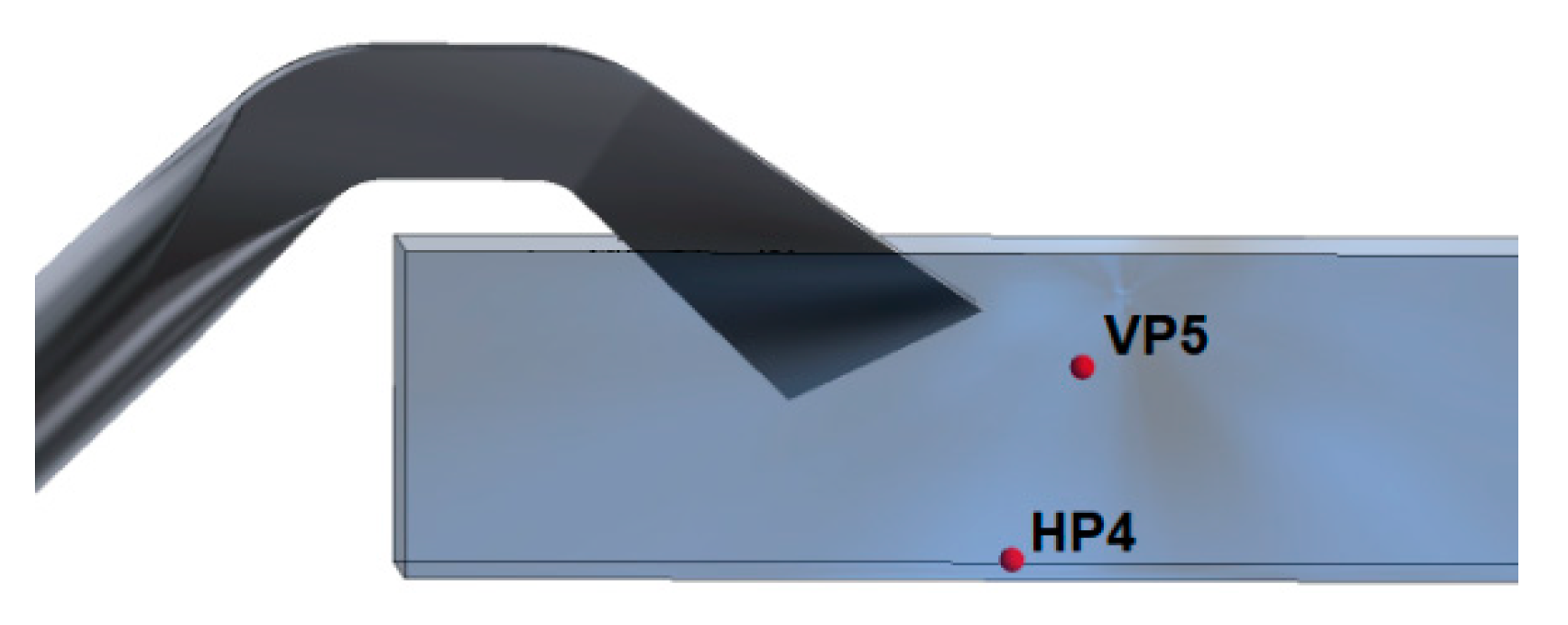
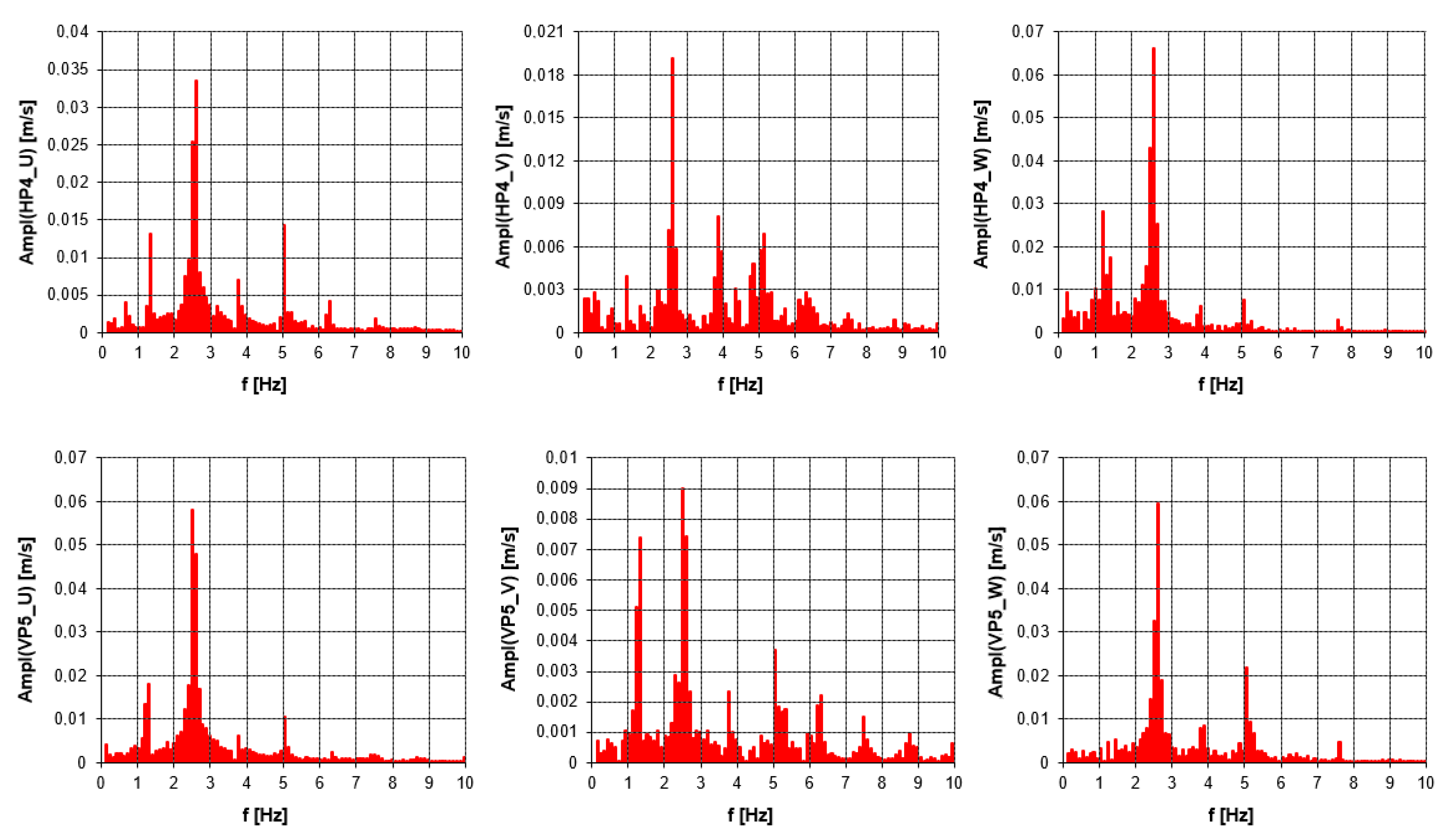
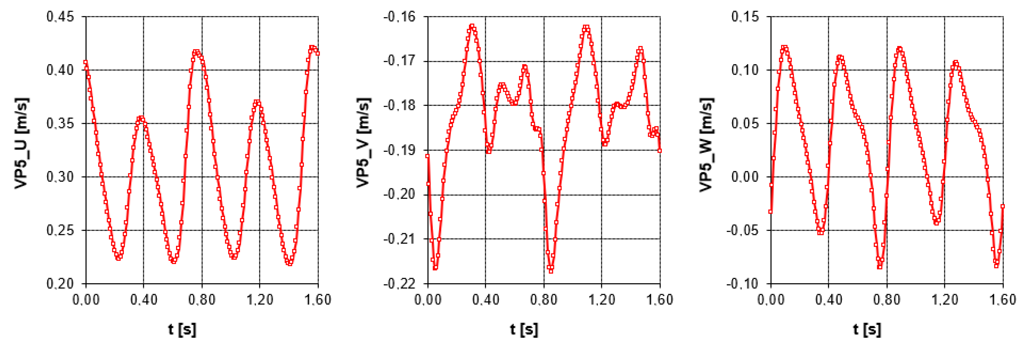
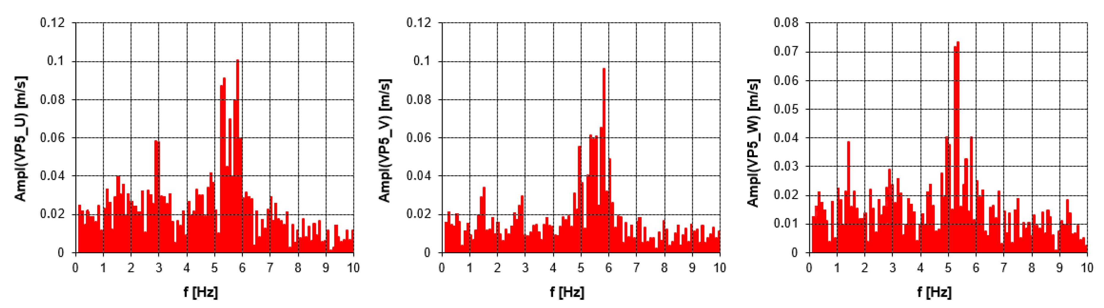
Therefore, so as to analyze frequencies linked to the unsteady phenomena in the computational domain, a system of ten control points has been used, in each all three velocity components being monitored. In this study, two most important points are presented. The point HP4 (with the coordinates x = 386 mm, y = 10 mm, z = 0 mm) is located in the symmetry line of the horizontal plane y = 10 mm, in the position where the nodal point of attachment moves (Figure 42). The point VP5 is located in the symmetry plane z = 0 mm, in the position, where vortices are shedding in the shear layer behind the upper siphon wall. Its coordinates are x = 465 mm, y = 164 mm, z = 0 mm. The numerical simulations based on the SST turbulence model show a distinct dominant frequency of 2.5 Hz in all control points. In addition, the frequencies 1.25 and 5 Hz are important, especially in the point VP5 (Figure 43). Graphs of velocity components during 1.6 s can be seen in Figure 44. The frequency analysis of the numerical simulations based on the SAS scale resolving simulations is much more “noisy”. In the point HP4, the dominant frequency is about 2.8–3 Hz, which is close to the SST results. However, in the point VP5, the dominant frequency is somewhere between 5 and 6.3 Hz (Figure 45), which is approximately a double frequency of the SST prediction. Nevertheless, this frequency obtained from the Fast Fourier Transform (hereinafter FFT) analysis of velocity components corresponds well with the visualizations in Figure 35.
6. Discussion
The goal of the study is to perform a validation of the mathematical model and to study the flow topology and dynamics in detail. The laboratory simplified model of the real situation was built up. The reason of using the simplified laboratory model is that the application of the advanced experimental techniques based on the optical principle is not possible in the real situation. In reality, the geometry of the discharge object can be more complicated [4], the size is bigger and the vessel walls are not suitable for the optical measurements (they are typically made of concrete). Nevertheless the flow phenomena investigated in the study depict the complex flow behavior enough to validate reliably the CFD tools used by authors.
The primary flow structure is the water jet, behind the siphon outlet, accompanied with the backflow and the strong vortex just below the siphon outlet. The nodal point of attachment (or a structure of connected unstable singular points) is unsteady and moves with the dominant frequency of several Hz. The dynamic and erosive effects of this structure should be considered during the design of the discharge object.
Comparisons of the SAS and SST simulations show a good agreement of the time-averaged flow fields, which also agree well with the visualizations by means of PIV. The SAS scale resolving simulations give more detailed view of all vortical structures, but the computational demands are much higher. Concerning the frequency analysis, predictions of the dominant frequency (related to the nodal point of attachment) from both numerical models differ about 10%, but the frequency chart from the SAS scale resolving simulations is much more “noisy” suggesting the higher frequencies resolved by this method.
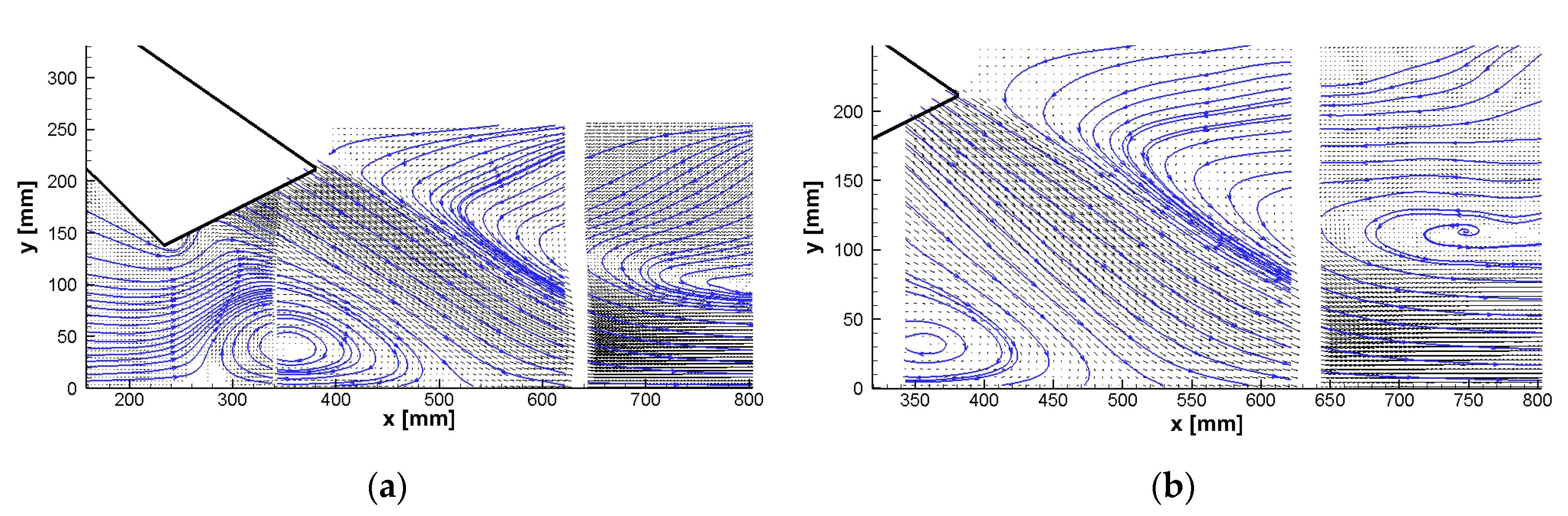
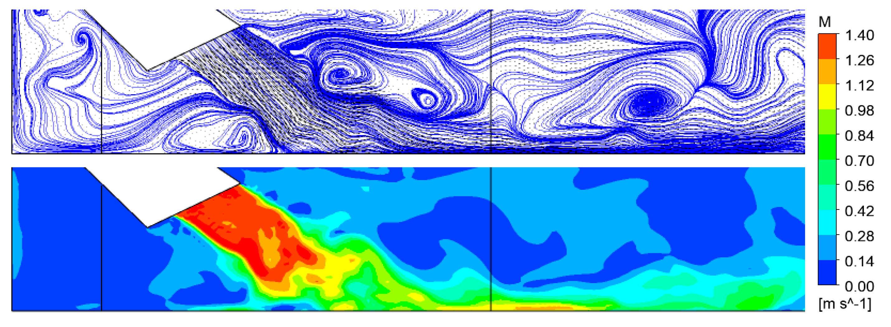
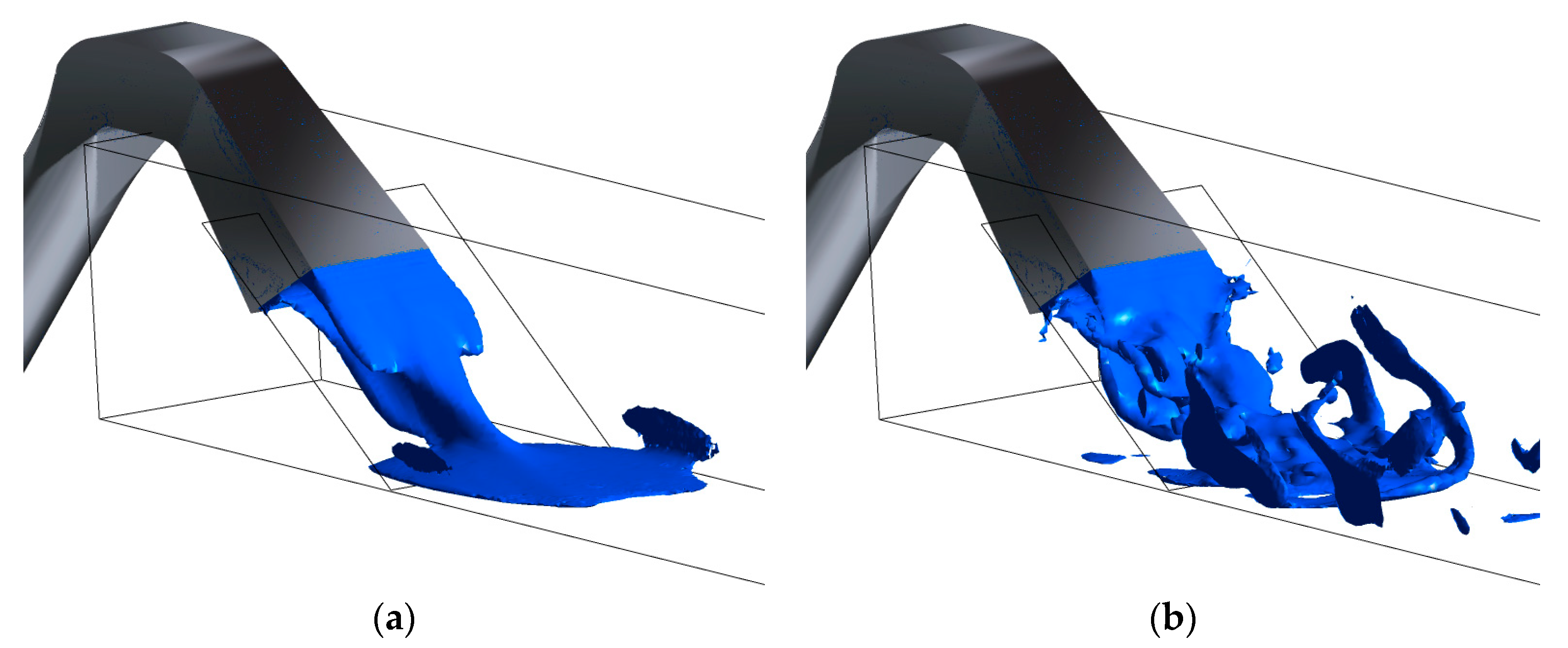
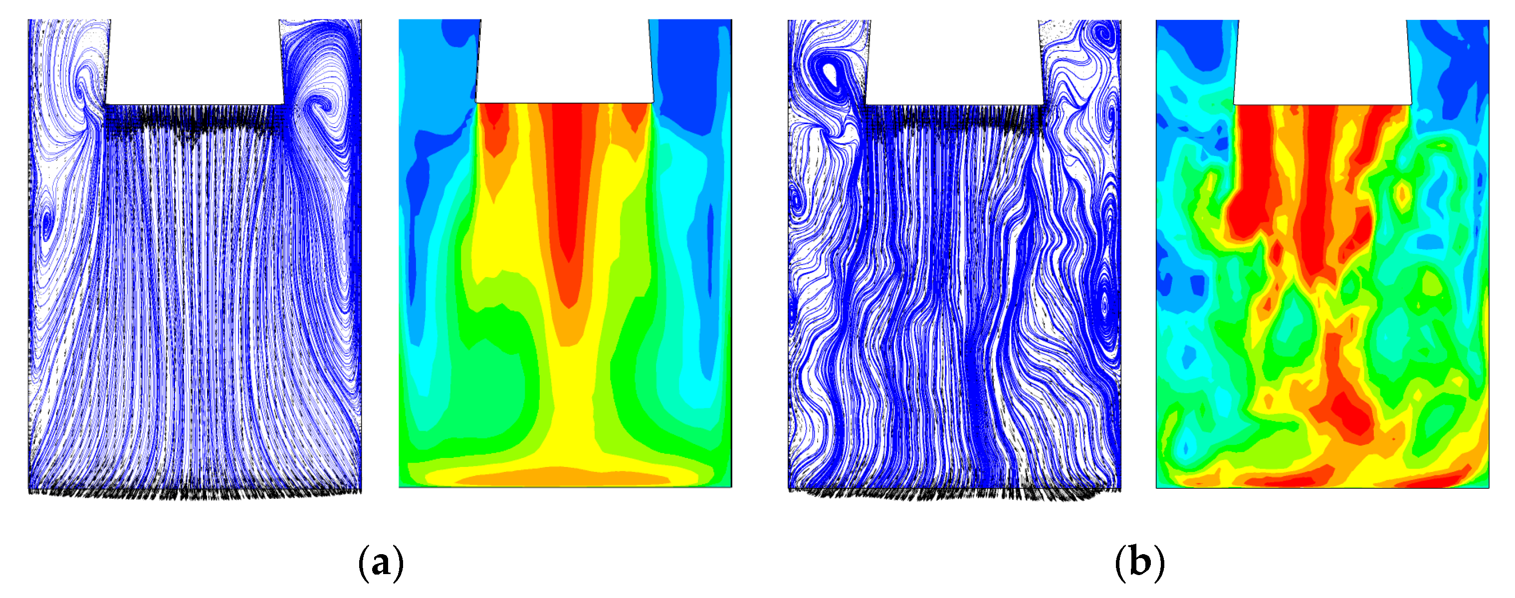
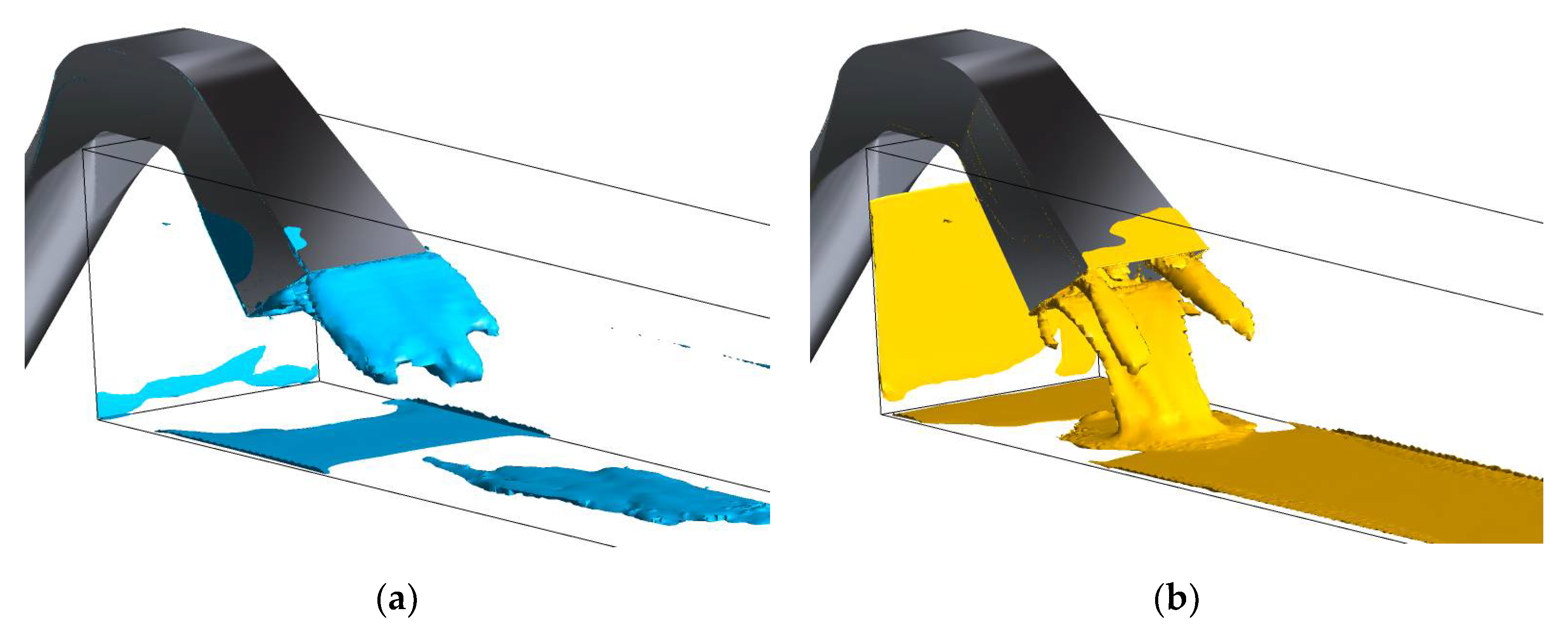
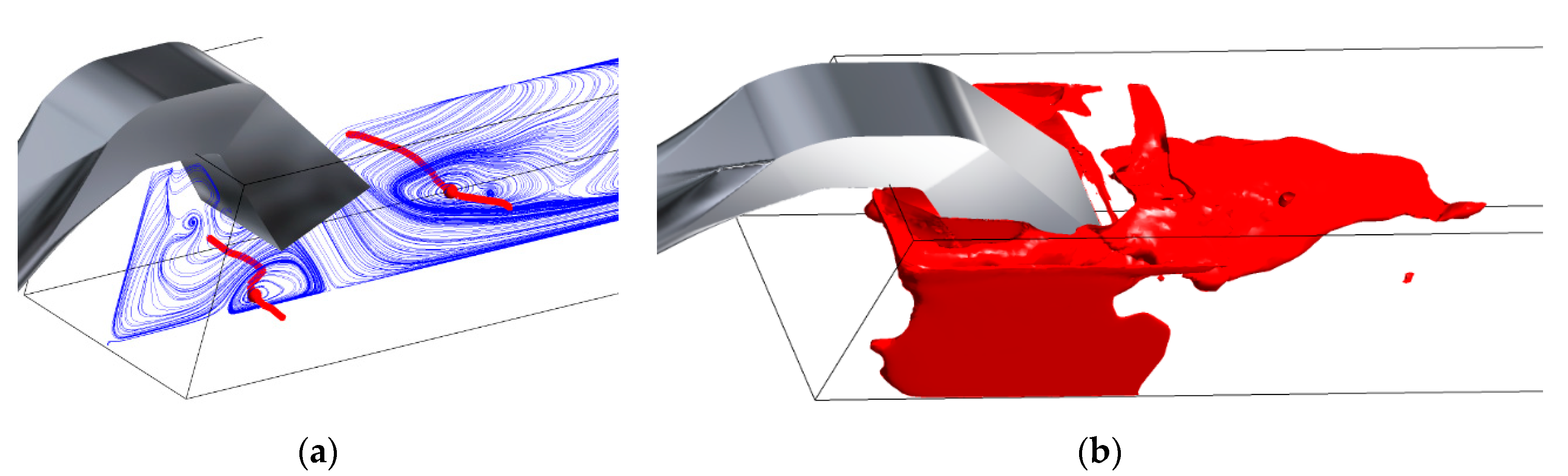
The methodology used in this study can be generally very effective to design and optimize the pump or turbine systems. When validated by the experimental data, the CFD tools enable to examine a wide range of variants and to choose the best one. CFD also provides very effective tools for the detailed analysis of the flow phenomena, their interaction and dynamics. Figure 46 shows the 3D view of the time-averaged and unsteady water jets behind the siphon outlet visualized for the SAS simulations. Figure 47 shows the (two-dimensional) magnitude of velocity and the vector lines in the inclined plane behind the siphon outlet, which follows the main part of the jet (as indicated in Figure 46). Two vortical structures close to the side walls are driven by the jet side shear layers. The shear layers which are the sources of two dominant vortices above and below the water jet are visualized in Figure 48 by means of the iso-surfaces with the opposite value of vorticity. Vortex filaments of these dominant vortices are shown in Figure 49a. It can be seen that these filaments are not straight and do not extend up to the side walls, as both the dominant vortices dissipate in the side boundary layers. The 3D view of the strong backflow region associated with these vortices can be seen in Figure 49b visualized by means of the iso-surfaces of the negative longitudinal velocity U = −0.17 m/s.
Still, the methodology limitations should be mentioned as well. First, there are limits of the experimental research. Measurements are done one by one in different planes and different measurement segments. That is why, only the time-averaged results can be used to reconstruct the complex 3D view of flow in the test section. Concerning the numerical methods, they are still limited by computational resources, especially in the case of calculations with advanced physical models. In many cases it is still not possible to use sufficiently dense computational grids and sufficiently long computational times, which can guarantee grid-independent and sufficiently time-averaged results.
7. Conclusions
The subject of the presented study is the laboratory model of a pumping system’s discharge object with the welded siphon and a relatively simple geometry of the discharge object. Results of both the experimental research and mathematical modelling are presented.
Two stationary flow regimes characterized by different volume flow rates and water level heights have been chosen. The study concentrates mainly on the regions below and behind the siphon outlet. Five vertical planes, three horizontal planes and one cross-wise section have been examined, focused mainly on the regions below and behind the siphon outlet. The experimental data are compared with the results of the CFD simulations, based on the ANSYS CFX software and the SST and SAS turbulence models.
The mathematical modelling using the advanced simulation methods has been performed, the volume-of-fluid method has been applied for the free-surface flow modelling. The experimental results obtained by the PIV method are used for the mathematical model validation. The presented results show a good agreement of measured and calculated complex flow topology below and behind the siphon outlet, especially close to the test-section floor.
The unsteady behavior of the flow from the siphon impinging to the vessel bottom has been observed and analyzed using the spectral methods. The evolution and interactions of the main flow structures have been studied using visualizations.
Nowadays, the CFD tools are able to model all the complete hydraulic system of a pumping or water turbine station, to prove the functionality and design parameters of hydrodynamic machines as well as to guarantee functionality of such a new station under design, as any changes and reconstructions of the suction and discharge objects of the station are extremely time and money consuming. The numerical models are not restricted to a simple geometry and can replace the physical modelling in the laboratory, which is (in a full complex geometry of the complete station) practically impossible. From this point of view, any improvement, validation and verification of the numerical tools, used for the optimal design of pumping or turbine stations, is highly desirable.
Author Contributions
Conceptualization, M.S., V.U. and M.K.; methodology, M.S., V.U., M.K. and P.P.; CFD, M.S.; PIV, P.P., V.U. and V.S.; validation M.S., P.P. and V.U.; resources, M.S. and V.U.; writing—original draft preparation, M.S. and P.P.; writing—review and editing, V.U.; visualization, P.P. and M.S.; supervision, M.S. and V.U.; project administration, M.S.; funding acquisition, M.S. All authors have read and agreed to the published version of the manuscript.
Funding
This research was funded by the Ministry of Industry and Trade of the Czech Republic under the grant project FV30104 “Suction and Discharge Objects of Pump and Turbine Stations”.
Conflicts of Interest
The authors declare no conflict of interest. The funders had no role in the design of the study; in the collection, analyses, or interpretation of data; in the writing of the manuscript, or in the decision to publish the results.
Nomenclature
| f | frequency [Hz] |
| h | height [m] or [mm] |
| l | length [m] or [mm] |
| M | magnitude of two-dimensional velocity vector [m/s] in specified plane |
| Q | velocity invariant (exact definition in [15]) [s−2] |
| Qv | volume flow rate [m3/s] or [L/s] |
| t | time [s] |
| U, V, W | velocity components [m/s] |
| W | width [m] or [mm] |
| x, y, z | Cartesian coordinates [m] or [mm] |
| y+ | dimensionless wall distance [-] |
| Δt | time step [s] |
| Abbreviations | |
| Amp | Amplitude |
| CFD | Computational Fluid Dynamics |
| CMOS | Complementary Metal–Oxide–Semiconductor |
| DES | Detached Eddy Simulations |
| DN | Diameter Nominal |
| FFT | Fast Fourier Transform |
| HP | Horizontal Plane |
| LES | Large Eddy Simulations |
| Nd:YLF | Neodymium-Doped Yttrium Lithium Fluoride |
| PIV | Particle Image Velocimetry |
| RANS | Reynolds-Averaged Navier–Stokes equations |
| SAS | Scale Adaptive Simulations |
| SST | Shear Stress Transport |
| URANS | Unsteady Reynolds-Averaged Navier–Stokes Equations |
| VOF | Volume of Fluid |
| VP | Vertical Plane |
References
- Zhu, H.; Zhu, G.; Lu, W.; Zhang, Y. Optimal Hydraulic Design and Numerical Simulation of Pumping Systems. Procedia Eng. 2012, 28, 75–80. [Google Scholar] [CrossRef] [Green Version]
- Sedlář, M.; Šoukal, J.; Krátký, T. Numerical analysis of hydraulic systems with free water level. In Proceedings of the 7th International Symposium on Fluid Machinery and Fluids Engineering, Jeju, Korea, 18–22 October 2016. [Google Scholar]
- Liu, Y.; Zhou, J.; Zhou, D. Transient flow analysis in axial-flow pump system during stoppage. Adv. Mech. Eng. 2017, 9, 1–8. [Google Scholar] [CrossRef] [Green Version]
- Sedlář, M.; Machalka, J.; Komárek, M. Modeling and Optimization of Multiphase Flow in Pump Station. J. Phys. Conf. Ser. 2020, 1584. [Google Scholar] [CrossRef]
- Tokay, T.; Constantinescu, G. Coherent structures in pump-intake flows; A Large Eddy Simulation (LES) study. In Proceedings of the XXXI IAHR Congres, Seoul, Korea, 11–16 September 2005. [Google Scholar]
- Okamura, T.; Kamemoto, J.; Matsui, J. CFD prediction and model experiment on suction vortices in pump sump. In Proceedings of the 9th Asian International Conference on Fluid Machinery, Jeju, Korea, 16–19 October 2007. [Google Scholar]
- Bayeul-Lainé, A.C.; Bois, G.; Issa, A. Numerical simulation of flow field in water-pump sump and inlet suction pipe. IOP Conf. Ser. Earth Environ. Sci. 2010, 12, 1–9. [Google Scholar] [CrossRef] [Green Version]
- Kim, C.G.; Kim, B.H.; Bang, B.H.; Lee, Y.H. Experimental and CFD analysis for prediction of vortex and swirl angle in the pump sump station model. IOP Conf. Ser. Mater. Sci. Eng. 2015, 72, 1–7. [Google Scholar] [CrossRef] [Green Version]
- Ajai, S.; Kumar, K.; Abdul Rahiman, P.M.; Sohoni, V.S.; Jahagirdar, V.S. Vortex prediction in a pump intake system using Computational Fluid Dynamics. IJITEE 2019, 8, 3158–3163. [Google Scholar] [CrossRef]
- Zhu, H.; Bo, G.; Zhou, Y.; Zhang, R.; Cheng, J. Performance prediction of pump and pumping system based on combination of numerical simulation and non-full passage model test. J. Braz. Soc. Mech. Sci. Eng. 2019, 41, 1–12. [Google Scholar] [CrossRef] [Green Version]
- Guo, M.; Zuo, Z.; Liu, S.; Zou, H.; Chen, B.; Li, D. Experimental Vortex Patterns in the primary and secondary pump intakes of a model underground pumping station. Energies 2020, 13, 1790. [Google Scholar] [CrossRef] [Green Version]
- Tobak, M.; Peake, D.J. Topology of Three-Dimensional Separated Flows. Annu. Rev. Fluid Mech. 1982, 14, 61–85. [Google Scholar] [CrossRef] [Green Version]
- Procházka, P.; Uruba, V. Streamwise and spanwise vortical structure merging inside the wake of an inclined flat plate. Mech. Ind. 2019, 20, 705. [Google Scholar] [CrossRef] [Green Version]
- Menter, F.R.; Schutze, J.; Kurbatskii, K.A. Scale-Resolving Simulation Techniques in Industrial CFD. In Proceedings of the 6th AIAA Theoretical Fluid Mechanics Conference, Honolulu, HI, USA, 27–30 June 2011; pp. 2011–3474. [Google Scholar] [CrossRef]
- Menter, F.R. Best Practice: Scale-Resolving Simulations in ANSYS CFD, Version 2; ANSYS Germany GmbH: Otterfing, Germany, 2015. [Google Scholar]
Figure 1.
Closed circuit with the test section and the open air tank.

Figure 2.
Experiment set-up. (a) Test section; (b) detail of the welded siphon.

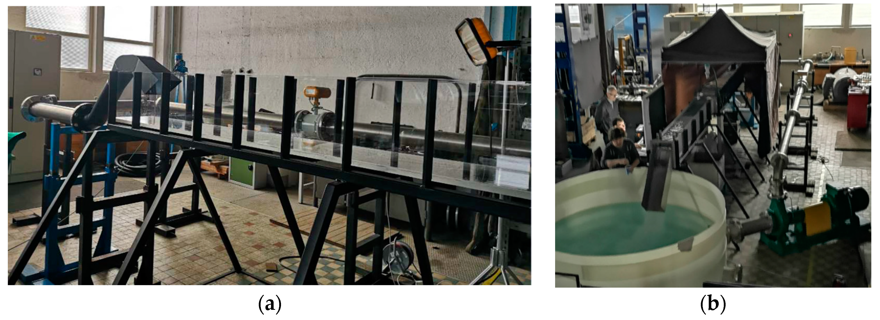
Figure 3.
(a) Detail of the transparent test sections; (b) arrangement of the particle image velocimetry (PIV) measurements with a blackout tent. Details of the water tank and water chute can be seen.
Figure 3.
(a) Detail of the transparent test sections; (b) arrangement of the particle image velocimetry (PIV) measurements with a blackout tent. Details of the water tank and water chute can be seen.

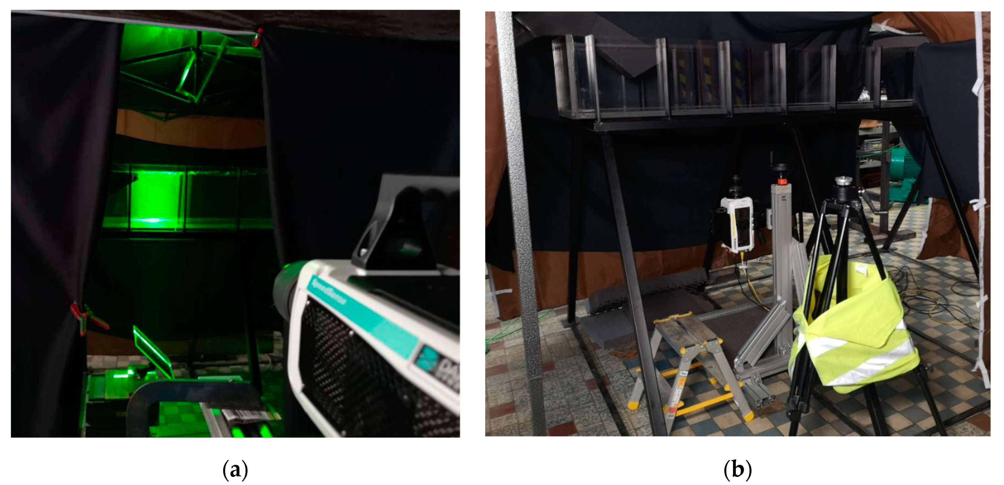
Figure 4.
(a) Measurements in vertical planes. Laser sheet is reflecting on the mirror in 45°; (b) position of the high-speed camera during measurements in horizontal planes.
Figure 4.
(a) Measurements in vertical planes. Laser sheet is reflecting on the mirror in 45°; (b) position of the high-speed camera during measurements in horizontal planes.

Figure 5.
Calibration of the camera view in vertical plane, Section B.

Figure 6.
Computational grid. (a) Surface mesh; (b) detail of the grid resolution in vertical plane z = 0 mm.
Figure 6.
Computational grid. (a) Surface mesh; (b) detail of the grid resolution in vertical plane z = 0 mm.

Figure 7.
Vertical plane z = 0 mm. (a) Velocity magnitude; (b) vector lines.

Figure 8.
Vertical plane z = 75 mm. (a) Velocity magnitude; (b) vector lines.

Figure 9.
Vertical plane z = −75 mm. (a) Velocity magnitude; (b) vector lines.

Figure 10.
Vertical planes in Sector C. (a) Velocity magnitude; (b) vector lines.

Figure 11.
Horizontal plane y = 10 mm. (a) Velocity magnitude; (b) vector lines.

Figure 12.
Horizontal plane y = 135 mm. (a) Velocity magnitude; (b) vector lines.

Figure 13.
Horizontal plane y = 170 mm. (a) Velocity magnitude; (b) vector lines.

Figure 14.
Instantaneous flow in horizontal plane y = 10 mm. (a) and (b); two different time instants. Vector lines and vorticity.
Figure 14.
Instantaneous flow in horizontal plane y = 10 mm. (a) and (b); two different time instants. Vector lines and vorticity.

Figure 15.
Flow in the shear layer behind the upper siphon wall in vertical plane z = 0 mm. Pictures and the coordinate system are rotated by 37° against the horizon. (a) Time-averaged velocity field; (b) instantaneous vortices behind the wall edge.
Figure 15.
Flow in the shear layer behind the upper siphon wall in vertical plane z = 0 mm. Pictures and the coordinate system are rotated by 37° against the horizon. (a) Time-averaged velocity field; (b) instantaneous vortices behind the wall edge.

Figure 16.
Vector lines. (a) Vertical plane z = 0 mm.; (b) vertical plane z = 75 mm. This is the only picture with the volume flow rate Qv = 0.0138 m3/s.
Figure 16.
Vector lines. (a) Vertical plane z = 0 mm.; (b) vertical plane z = 75 mm. This is the only picture with the volume flow rate Qv = 0.0138 m3/s.

Figure 17.
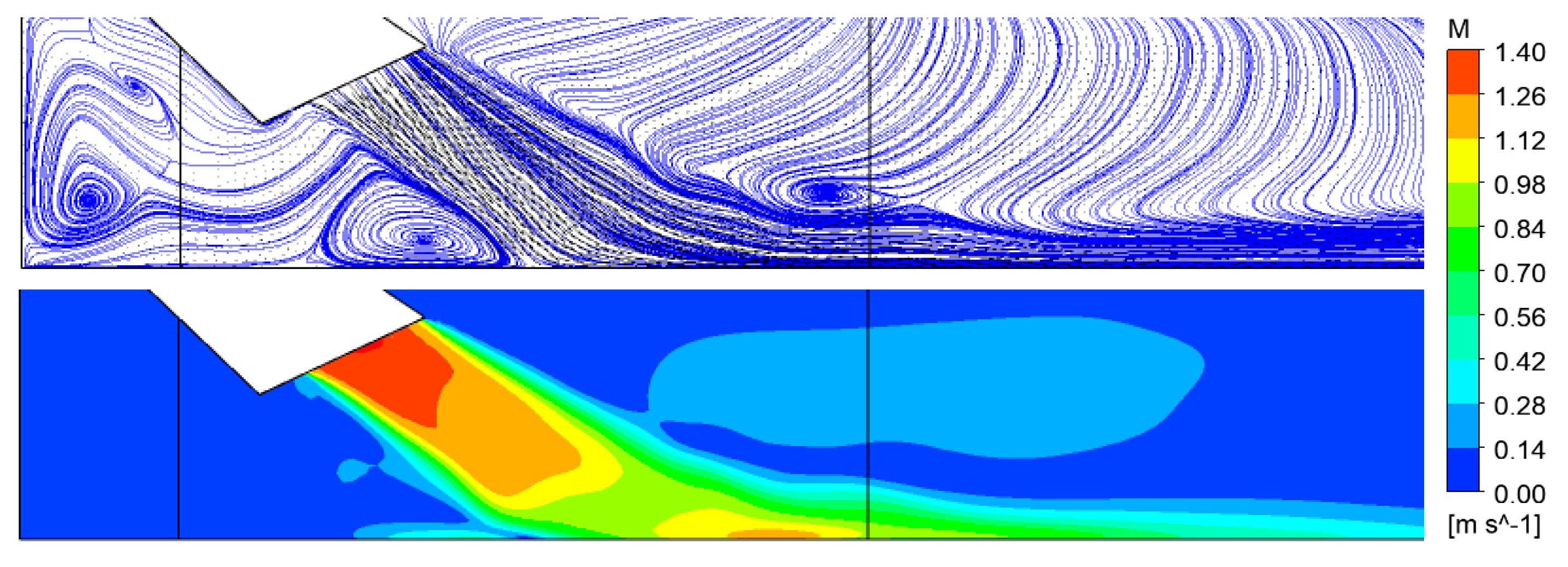
Time averaged scale-adaptive simulation (SAS). Vertical plane z = 0 mm. Vector lines (top), 2D velocity magnitude (bottom).
Figure 17.
Time averaged scale-adaptive simulation (SAS). Vertical plane z = 0 mm. Vector lines (top), 2D velocity magnitude (bottom).

Figure 18.
Time averaged SAS simulation. Vertical plane z = 75 mm. Vector lines (top), 2D velocity magnitude (bottom).
Figure 18.
Time averaged SAS simulation. Vertical plane z = 75 mm. Vector lines (top), 2D velocity magnitude (bottom).

Figure 19.
Time averaged SAS simulation. Vertical plane z = −75 mm. Vector lines (top), 2D velocity magnitude (bottom).
Figure 19.
Time averaged SAS simulation. Vertical plane z = −75 mm. Vector lines (top), 2D velocity magnitude (bottom).

Figure 20.
Time averaged SAS simulation. Vertical plane z = 141 mm. Vector lines (top), 2D velocity magnitude (bottom).
Figure 20.
Time averaged SAS simulation. Vertical plane z = 141 mm. Vector lines (top), 2D velocity magnitude (bottom).

Figure 21.
Time averaged SAS simulation. Vertical plane z = −141 mm. Vector lines (top), 2D velocity magnitude (bottom).
Figure 21.
Time averaged SAS simulation. Vertical plane z = −141 mm. Vector lines (top), 2D velocity magnitude (bottom).

Figure 22.
Time averaged shear stress transport (SST) simulation. Vertical plane z = 0 mm. Vector lines (top), 2D velocity magnitude (bottom).
Figure 22.
Time averaged shear stress transport (SST) simulation. Vertical plane z = 0 mm. Vector lines (top), 2D velocity magnitude (bottom).

Figure 23.
Time averaged SST simulation. Vertical plane z = 75 mm. Vector lines (top), 2D velocity magnitude (bottom).
Figure 23.
Time averaged SST simulation. Vertical plane z = 75 mm. Vector lines (top), 2D velocity magnitude (bottom).

Figure 24.
Time averaged SST simulation. Vertical plane z = −75 mm. Vector lines (top), 2D velocity magnitude (bottom).
Figure 24.
Time averaged SST simulation. Vertical plane z = −75 mm. Vector lines (top), 2D velocity magnitude (bottom).

Figure 25.
Time averaged SST simulation. Vertical plane z = 141 mm. Vector lines (top), 2D velocity magnitude (bottom).
Figure 25.
Time averaged SST simulation. Vertical plane z = 141 mm. Vector lines (top), 2D velocity magnitude (bottom).

Figure 26.
Time averaged SST simulation. Vertical plane z = −141 mm. Vector lines (top), 2D velocity magnitude (bottom).
Figure 26.
Time averaged SST simulation. Vertical plane z = −141 mm. Vector lines (top), 2D velocity magnitude (bottom).

Figure 27.
Time averaged SAS simulation. Horizontal plane y = 10 mm. Vector lines (top), 2D velocity magnitude (bottom).
Figure 27.
Time averaged SAS simulation. Horizontal plane y = 10 mm. Vector lines (top), 2D velocity magnitude (bottom).

Figure 28.
Time averaged SAS simulation. Horizontal plane y = 135 mm. Vector lines (top), 2D velocity magnitude (bottom).
Figure 28.
Time averaged SAS simulation. Horizontal plane y = 135 mm. Vector lines (top), 2D velocity magnitude (bottom).

Figure 29.
Time averaged SAS simulation. Horizontal plane y = 170 mm. Vector lines (top), 2D velocity magnitude (bottom).
Figure 29.
Time averaged SAS simulation. Horizontal plane y = 170 mm. Vector lines (top), 2D velocity magnitude (bottom).

Figure 30.
Time averaged SST simulation. Horizontal plane y = 10 mm. Vector lines (top), 2D velocity magnitude (bottom).
Figure 30.
Time averaged SST simulation. Horizontal plane y = 10 mm. Vector lines (top), 2D velocity magnitude (bottom).

Figure 31.
Time averaged SST simulation. Horizontal plane y = 135 mm. Vector lines (top), 2D velocity magnitude (bottom).
Figure 31.
Time averaged SST simulation. Horizontal plane y = 135 mm. Vector lines (top), 2D velocity magnitude (bottom).

Figure 32.
Time averaged SST simulation. Horizontal plane y = 170 mm. Vector lines (top), 2D velocity magnitude (bottom).
Figure 32.
Time averaged SST simulation. Horizontal plane y = 170 mm. Vector lines (top), 2D velocity magnitude (bottom).

Figure 33.
SAS simulation. Time instant t0 + 2.92 s. Vertical plane z = 0 mm. Vector lines (top), 2D velocity magnitude (bottom).
Figure 33.
SAS simulation. Time instant t0 + 2.92 s. Vertical plane z = 0 mm. Vector lines (top), 2D velocity magnitude (bottom).

Figure 34.
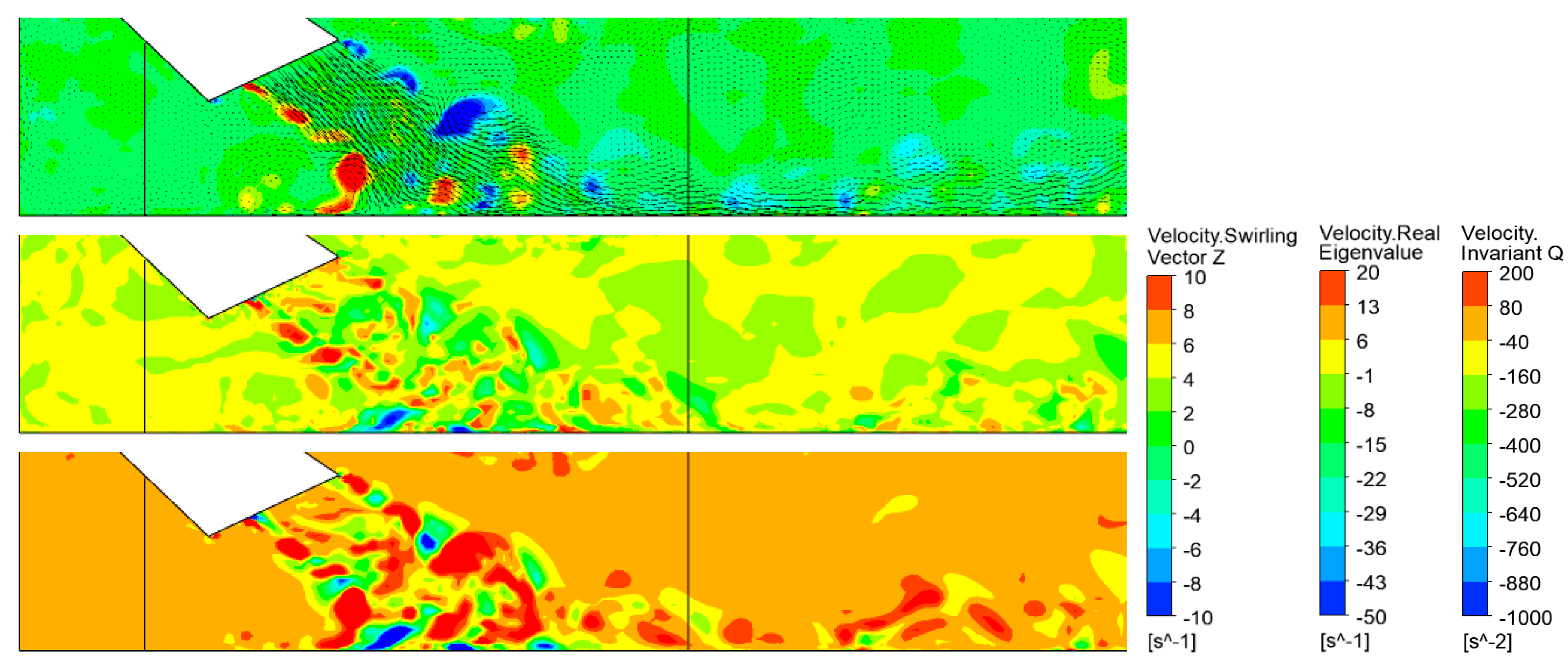
SAS simulation. Time instant t0 + 2.92 s. Vertical plane z = 0 mm. Vorticity (top), velocity real eigenvalue (middle) and Q invariant (bottom).
Figure 34.
SAS simulation. Time instant t0 + 2.92 s. Vertical plane z = 0 mm. Vorticity (top), velocity real eigenvalue (middle) and Q invariant (bottom).

Figure 35.
SAS simulation. Unsteady vortices behind the siphon edge. Vertical plane z = 0 mm. Vector lines.
Figure 35.
SAS simulation. Unsteady vortices behind the siphon edge. Vertical plane z = 0 mm. Vector lines.

Figure 36.
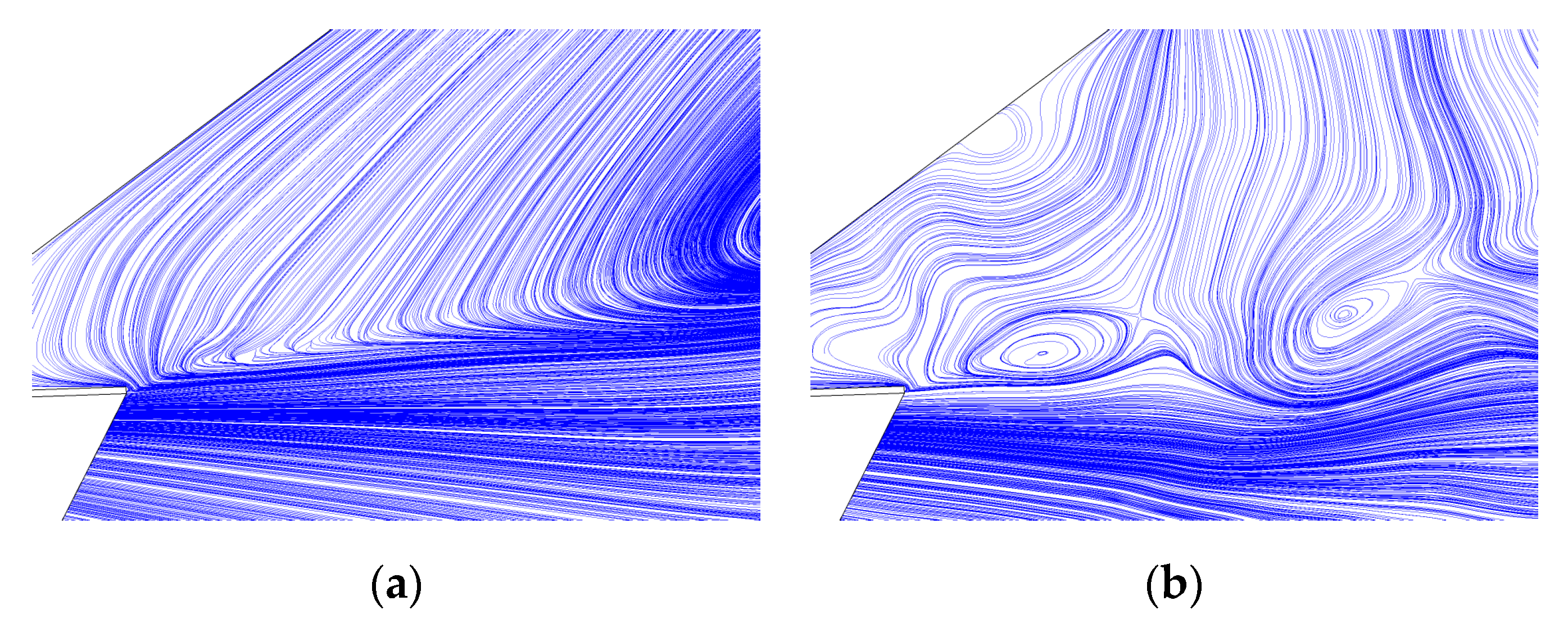
SAS Simulation. Flow in the shear layer behind the upper siphon wall in vertical plane z = 0 mm. Pictures and the coordinate system are rotated by 37° against the horizon. (a) Time-averaged velocity field; (b) unsteady vortices behind the wall edge.
Figure 36.
SAS Simulation. Flow in the shear layer behind the upper siphon wall in vertical plane z = 0 mm. Pictures and the coordinate system are rotated by 37° against the horizon. (a) Time-averaged velocity field; (b) unsteady vortices behind the wall edge.

Figure 37.
SST simulation. Time instant t0 + 5.96 s. Vertical plane z = 0 mm. Vector lines (top), 2D velocity magnitude (bottom).
Figure 37.
SST simulation. Time instant t0 + 5.96 s. Vertical plane z = 0 mm. Vector lines (top), 2D velocity magnitude (bottom).

Figure 38.
SAS simulation. Time instant t0 + 2.92 s. Horizontal plane y = 10 mm. Vector lines (top), 2D velocity magnitude (bottom).
Figure 38.
SAS simulation. Time instant t0 + 2.92 s. Horizontal plane y = 10 mm. Vector lines (top), 2D velocity magnitude (bottom).

Figure 39.
SAS simulation. Time instant t0 + 2.92 s. Horizontal plane y = 10 mm. Vorticity (top), velocity real eigenvalue (middle) and Q invariant (bottom).
Figure 39.
SAS simulation. Time instant t0 + 2.92 s. Horizontal plane y = 10 mm. Vorticity (top), velocity real eigenvalue (middle) and Q invariant (bottom).

Figure 40.
SST simulation. Time instant t0 + 5.96 s. Horizontal plane y = 10 mm. Vector lines (top), 2D velocity magnitude (bottom).
Figure 40.
SST simulation. Time instant t0 + 5.96 s. Horizontal plane y = 10 mm. Vector lines (top), 2D velocity magnitude (bottom).

Figure 41.
SST simulation. Unsteady vortices behind the siphon edge. Horizontal plane y = 10 mm.

Figure 42.
Control points for FFT analysis of velocity components. Point HP4 representing horizontal plane y = 10 mm, point VP5 representing vertical plane z = 0 mm.
Figure 42.
Control points for FFT analysis of velocity components. Point HP4 representing horizontal plane y = 10 mm, point VP5 representing vertical plane z = 0 mm.

Figure 43.
FFT analysis of velocity components in horizontal plane y = 10 mm, point HP4 (top) and vertical plane z = 0 mm, point VP5 (bottom). CFD simulation, SST model.
Figure 43.
FFT analysis of velocity components in horizontal plane y = 10 mm, point HP4 (top) and vertical plane z = 0 mm, point VP5 (bottom). CFD simulation, SST model.

Figure 44.
Velocity component in vertical plane z = 0 mm, point VP5 during 1.6 s. CFD simulation, SST model.
Figure 44.
Velocity component in vertical plane z = 0 mm, point VP5 during 1.6 s. CFD simulation, SST model.

Figure 45.
FFT analysis of velocity components in vertical plane z = 0 mm, point VP5. CFD simulation, SAS model.
Figure 45.
FFT analysis of velocity components in vertical plane z = 0 mm, point VP5. CFD simulation, SAS model.

Figure 46.
SAS Simulation. 3D view of the water jet behind the siphon outlet visualized with iso-surfaces of the 3D velocity magnitude 1 m/s. (a) Time-averaged velocity field; (b) unsteady flow, time instant t0 + 2.92 s.
Figure 46.
SAS Simulation. 3D view of the water jet behind the siphon outlet visualized with iso-surfaces of the 3D velocity magnitude 1 m/s. (a) Time-averaged velocity field; (b) unsteady flow, time instant t0 + 2.92 s.

Figure 47.
SAS simulation. Vector lines and 2D velocity magnitude in the inclined plane behind the siphon outlet. Pictures and the coordinate system are rotated by 35° against the horizon. (a) Time-averaged velocity field; (b) unsteady flow, time instant t0 + 2.92 s.
Figure 47.
SAS simulation. Vector lines and 2D velocity magnitude in the inclined plane behind the siphon outlet. Pictures and the coordinate system are rotated by 35° against the horizon. (a) Time-averaged velocity field; (b) unsteady flow, time instant t0 + 2.92 s.

Figure 48.
SAS Simulation. 3D view of the time-averaged vorticity Z component behind the siphon outlet visualized with iso-surfaces. (a) Value −20 s−1; (b) value 20 s−1.
Figure 48.
SAS Simulation. 3D view of the time-averaged vorticity Z component behind the siphon outlet visualized with iso-surfaces. (a) Value −20 s−1; (b) value 20 s−1.

Figure 49.
SAS Simulation. (a) Time-averaged vortex core filaments (in red) of two dominant vortices; (b) 3D view of the time-averaged backflow regions visualized with iso-surfaces of negative longitudinal velocity U = −0.17 m/s.
Figure 49.
SAS Simulation. (a) Time-averaged vortex core filaments (in red) of two dominant vortices; (b) 3D view of the time-averaged backflow regions visualized with iso-surfaces of negative longitudinal velocity U = −0.17 m/s.

Publisher’s Note: MDPI stays neutral with regard to jurisdictional claims in published maps and institutional affiliations. |
© 2020 by the authors. Licensee MDPI, Basel, Switzerland. This article is an open access article distributed under the terms and conditions of the Creative Commons Attribution (CC BY) license (http://creativecommons.org/licenses/by/4.0/).
Share and Cite
MDPI and ACS Style
Sedlář, M.; Procházka, P.; Komárek, M.; Uruba, V.; Skála, V. Experimental Research and Numerical Analysis of Flow Phenomena in Discharge Object with Siphon. Water 2020, 12, 3330. https://0-doi-org.brum.beds.ac.uk/10.3390/w12123330
AMA Style
Sedlář M, Procházka P, Komárek M, Uruba V, Skála V. Experimental Research and Numerical Analysis of Flow Phenomena in Discharge Object with Siphon. Water. 2020; 12(12):3330. https://0-doi-org.brum.beds.ac.uk/10.3390/w12123330
Chicago/Turabian StyleSedlář, Milan, Pavel Procházka, Martin Komárek, Václav Uruba, and Vladislav Skála. 2020. "Experimental Research and Numerical Analysis of Flow Phenomena in Discharge Object with Siphon" Water 12, no. 12: 3330. https://0-doi-org.brum.beds.ac.uk/10.3390/w12123330
Note that from the first issue of 2016, this journal uses article numbers instead of page numbers. See further details here.